Article

Vertical Transportation Diversity of Petroleum Pollutants under Groundwater Fluctuations and the Instructions for Remediation Strategy

1
College of New Energy and Environment, Jilin University, Changchun 130021, China
2
No.111 Gecological Party, Guizhou Bureau of Geology and Mineral Exploration & Development, Guiyang 550081, China
3
School of Resource and Environment Engineering, Guizhou Institute of Technology, Guiyang 550003, China
*
Author to whom correspondence should be addressed.
Sustainability 2023, 15(8), 6514; https://doi.org/10.3390/su15086514
Submission received: 2 February 2023 / Revised: 31 March 2023 / Accepted: 10 April 2023 / Published: 12 April 2023
(This article belongs to the Section Pollution Prevention, Mitigation and Sustainability)

Abstract

:
Based on the information from an actual petroleum-contaminated site, a one-dimensional soil column was used to examine the vertical transportation diversities of different petroleum components under the influence of water table fluctuations, and the results revealed the following: (1) There were two obvious pollution accumulation zones under the condition of water table fluctuations: (i) The pollution infiltration zone dominated by the residual phase was formed at the leakage position, and (ii) the floating zone dominated by the free phase was formed near the water table. Combined with the viscosity of the organic components, the concentrations of the residual phase were octanoic acid > hexadecane > cyclohexane > toluene. Compared to coarse sand, clay can adsorb more components. (2) Different fluctuation frequencies had a great influence on the migration process of components. The free phase can transfer into the residual phase during the low groundwater table fluctuation. In the case of high-frequency groundwater fluctuations, there were more free phase components that can be carried by the water flow. However, due to the continuous flushing by the water, pollutants were finally spread to the whole underground system. (3) A cost-effectiveness remediation strategy is based on the difference in pollutant transportation. Therefore, the conclusions in this paper are fully applied in the actual contaminated sites. Specifically, the air-sparing (AS) and soil vapor extraction (SVE) devices were installed in the vadose zone to remove volatile substances (such as toluene). The permeable reactive barriers (PRBs) were set in the groundwater fluctuation zone to repair the residual pollutants (alkanes, cyclane, and asphaltenes hydrocarbons) that are continuously converted from the residual phase to the dissolved phase and free phase due to water level fluctuations. Hence, the results of this study provided a specific, targeted, and comprehensive strategy for petroleum pollution treatment.

1. Introduction

The issue of petroleum-contaminated groundwater during oil drilling, transportation, and storage has been extensively reported worldwide, attracting high levels of attention [1,2,3,4]. When petroleum components are accidentally released into the environment, organic substances with mutagenesis, carcinogenesis, and teratogenesis effects can enter the environment, causing extremely severe threats to human health and the ecological environment [5,6,7,8]. As one of the world’s largest oil producers and consumers, oil pollution in the soil and groundwater in China is a serious problem [9,10]. According to statistics, China’s petrochemical industry produces about 700,000 tons of crude oil each year, of which about 10% will enter the soil environment [11]. According to the survey from the National Soil Pollution Status Investigation Announcement, 16.1% of the tested soils exceeded the standard of organic pollutants [12,13].
Crude oil is a multicomponent mixture that can be roughly divided into four categories: saturated hydrocarbons (n-alkanes, iso-alkanes, and naphthenes, etc.), aromatic hydrocarbons (monocyclic aromatic hydrocarbons and polycyclic aromatic hydrocarbons, etc.), gums (complexes composed of pyrimidines, quinolines, carbazoles, thiophenes, sulfoxides, and amino compounds), and asphaltenes (naphthenic acids, sulfides, polyphenols, fatty acids, metalloporphyrins, etc.). The physicochemical properties of petroleum organic components vary greatly. The American Petroleum Institute (API) tested the physicochemical properties of 478 organic substances obtained from crude oil refining, and the obtained data showed that substances with different organic functional groups had large differences in parameters such as solubility in water, Henry’s constant, and n-octanol water partition coefficient [14]. For example, the Henry constant of n-hexane is 68.38 at 25 °C, while cyclohexane (belonging to the same alkane) is 7.8, and the Henry constant of benzene, which also has the same number of carbon atoms, is 0.25, reflecting a huge difference in volatility. Hence, research on the behaviors of individual crude oil compounds is becoming increasingly popular. For example, Song et al. divided petroleum into saturated hydrocarbons and aromatic hydrocarbons and experimentally analyzed the degradation kinetics of these two organic compounds using microorganisms. The experimental results showed that the degradation effect of the microorganisms was quite different between the two [15]. Because of the wide variation in remediation relative to other traditional monotypes of pollutants, treating petroleum pollutants as a single type of substance is bound to produce inaccurate assessments. Therefore, whether an on-site survey or an indoor simulation experiment is conducted, it is necessary to conduct separate studies for different types of pollutants.
Other factor involved in the complex behavior of the components of crude oil are progresses such as convection, dispersion, adsorption, and volatilization, which complicate the determination and evaluation of the pollution process and result in difficulties in removal [16]. More specifically, as shown in Figure 1, groundwater, as an active agent, can carry petroleum components from the surface, spill spot, and transportation in the underground area [6,17,18]. During this journey, there is a special zone called the groundwater table fluctuation zone, where the groundwater table fluctuates as water is recharged and discharged, which causes the frequent conversions between the saturated zone and unsaturated zone (or vadose zone) [19,20]. The components of oil exist in three phases (Figure 1): the dissolved phase, the free phase, and the residual phase. The dissolved phase refers to the phase in which a substance is dissolved in water and migrates with the water. The free phase is the phase that exists in the soil pore space and floats on the water body as “oil bubbles” due to its poor solubility. This phase can move freely as an independent unit. The residual phase refers to the phase in which the petroleum component is confined in pores and struggles to move freely after binding to the soil grain with the adsorptive property and glutinousness [21,22]. Research on crude oil contamination under groundwater table fluctuations has been widespread, and the main information obtained is shown in Table 1.
In such a special zone, the redistribution of the petroleum component is governed by the changes in the water content caused by the fluctuating groundwater table and other environmental factors [34,35,36]. At the beginning of the release of crude oil, the oil floating on the water’s surface will continue to adhere to the soil when the water level drops, and when the water level is restored, the attached oil will be dissolved. Similarly, after the water level rises, the oil will remain in the vadose zone. When the water table rises, it will provide NAPL with buoyancy, allowing it to float; otherwise, it will be discharged downward due to gravity [37,38]. The petroleum components attached to the soil will be constantly dissolved and transported with the groundwater table, allowing for them to vertically combine with different environmental conditions to form the distributional difference or lateral diffusion. Therefore, the fluctuations in the water table expand the scope of oil pollution [39,40].
Oostorm et al. studied the distribution of pollutants from the source to the soil and groundwater under water-level fluctuations by simulating the migration of pollutants in a two-dimensional indoor sandbox. The experimental results showed that the pollutants originally stored in the soil of the vadose zone were transported with the infiltration water and continuously dissolved as the groundwater table rose, which was the main reason for the increased pollution in the groundwater [41]. Miller et al. constructed a mathematical model for calculating the thickness of the residual phase according to the relationship between the capillary pressure and the saturation of pollutants, obtaining good prediction results [42]. In addition to its influence on the concentration of the water-soluble phase, the fluctuations in the water table led to changes in the gas saturation levels in pores, as well as changes in the gas-phase concentration. Roy et al. studied the migration process of gas-phase pollutants under the condition of water table fluctuations. They indicated that the change in the discontinuous gas phase in pores mainly came from a change in the surface tension in the process of groundwater table fluctuations, which broke the original balance and changed the gas-phase saturation, resulting in the lateral diffusion of gas along the direction of the groundwater flow, or volatilization to the upper part of the vadose zone [43].
An accurate understanding of the multiple physical–chemical–biological reaction processes and the mutual transformation between dissolved, volatilized, and adsorbed NAPL pollution components is an essential premise for remediating groundwater petroleum pollution in a reasonable, efficient, and cost-effective manner during the water table fluctuation process. However, the influence mechanisms for individual petroleum pollutants caused by water table fluctuations and environmental processes in the fluctuation zone remain poorly researched. Therefore, based on a hydrogeological survey of the actual site pollution, this paper used groundwater table fluctuations as the environmental background of the pollution components to (1) investigate the vertical transportation diversities of different pollution components in the soil and groundwater system; (2) examine the influence of groundwater table fluctuations; and (3) explore cost-effective remediation strategies for crude-oil-contaminated sites.

2. Materials and Methods

2.1. Experimental Pollutants and Soil Media

2.1.1. Experimental Pollutants

According to the GC-MS analysis of the pollutants in the contaminated oilfield (Figure 2), there were four main types of organic pollutants: chainalkane hydrocarbons (Chs), cycloalkane hydrocarbons (Cys), aromatic hydrocarbons (Ars), and asphaltenes hydrocarbons (Aps). Hence, this simulation experiment selected hexadecane, cyclohexane, toluene, and octanoic acid as the typical components of these four types of pollutants (see Table 2 for their basic properties) to simulate different homogeneous soil columns (each soil column is made up of only one soil type) for petroleum contamination and to compare the migration and differentiation laws.

2.1.2. Experimental Soil Media and Device

In order to make the simulation experiment close to the real contaminated site conditions, two types of soil media (coarse sand and clay) were used according to the profile of the vadose zone and the shallow aquifer (Figure 3). The characteristics of the coarse sand and clay are displayed in Figure 4 and Table 3. In order to revive the real contaminated site conditions, soil media were evenly filled over the soil column to make sure the density was the same as the real condition (Table 3). Additionally, the water was injected into the tube from bottom to top, and then recharged until the water table was maintained to create a profile of the vadose zone and shallow aquifer. Both column 1 (filled with coarse sand) and column 2 (filled with clay) were filled with one homogenous soil. The experimental device was composed of polymethyl methacrylate and measured 100 cm in height and 10 cm in diameter. On the lateral face, there were 18 sampling and monitoring holes, separated by 5 cm (Figure 5). The total packing height was 90 cm.

2.2. Simulation Design of the Water Table Fluctuation Zone

By referring to the reported soil media and groundwater fluctuation amplitudes of different oil-contaminated sites of different countries, and based on the real contaminated oilfield of this research site, water table fluctuation zone, and soil column height, the initial water table was set at 40 cm. The water table fluctuated by 20 cm to the upper and lower sides, meaning that the water table fluctuation zone was 40 cm (Figure 6). The peristaltic pump was chosen to regulate the rate of the water table changes. In order to simulate an aquifer, the water was saturated from the bottom to the top, and the water table was determined based on the head value in the piezometric tube. The water saturation should be carried out slowly, ensuring that no bubbles exist in the aquifer.
In the experiment, the peristaltic pump was used to regulate the fluctuating water table. Two pumping methods were available, and the pumping rate was adjustable. When the water table rises, the water pump transfers water from the left-side water regulating tank to the right-side tank. When the water table falls, the opposite action must be taken. Since the water table fluctuation frequency at the actual site varied during the high-water period, normal-water period, and low-water period, three water table fluctuation frequencies were set in the experiment: 10 cm/h, 5 cm/h, and 2.5 cm/h. The water table in the entire soil column was measured using a piezometer tube, and Figure 7 exhibits the specific water table fluctuation control.

2.3. Adding Mode of Pollutants

In order to simulate the accidental release of crude oil in the oilfield, the initial content of the pollution components and the position were set according to Figure 2. First, the average concentrations of four types of pollutants were 2.5~21.0 g/kg in soil. Second, the total packing weights were 12.94 kg and 10.75 kg for coarse sand and clay, respectively. Hence, 50 mL (38.65 g, 38.95 g, 43.30 g, and 45.55 g of hexadecane, cyclohexane, toluene, and octanoic acid, respectively) of the individual component was injected into the interface of the water table through a thin glass tube. The Sudan IV staining tracing method was also used to observe the changes in the pollution halos during the whole experiment [44].

2.4. Sample Collection and Test Analysis

(1)
Soil sampling: During the experiment, soil in the column was taken out, and the infiltration of groundwater was changed, which caused inconsistencies in the simulation. Therefore, parallel experiments were designed. More specifically, experiments on four columns filled with coarse sand were conducted simultaneously under the same conditions. The columns were numbered column 1-1, column 1-2, column 1-3, and column 1-4. The experiment in column 1-1 was terminated after six hours, while the experiments in columns 2, 3, and 4 continued. Then, column 1-1 was unpacked, and soil samples were collected from various layers for measurement. Figure 5 presents S1, S2, and S3 as samples from the aquifer; V1 and V2 as samples from the vadose zone; and F1, F2, and F3 as samples from the fluctuation zone. Similarly, the experiment in column 1-2 was terminated after 32 h, while columns 1-3 and 1-4 continued. Using the sampling method described above, the columns filled with clay (column 2-1, column 2-2, column 2-3, and column 2-4) were collected in the same way as the coarse sand columns. These settings ensured that the soil media were not disturbed and that the experimental conditions did not change with soil sampling. The sampling times for the four soil columns were 6 h, 32 h, 82 h, and 110 h, respectively.
(2)
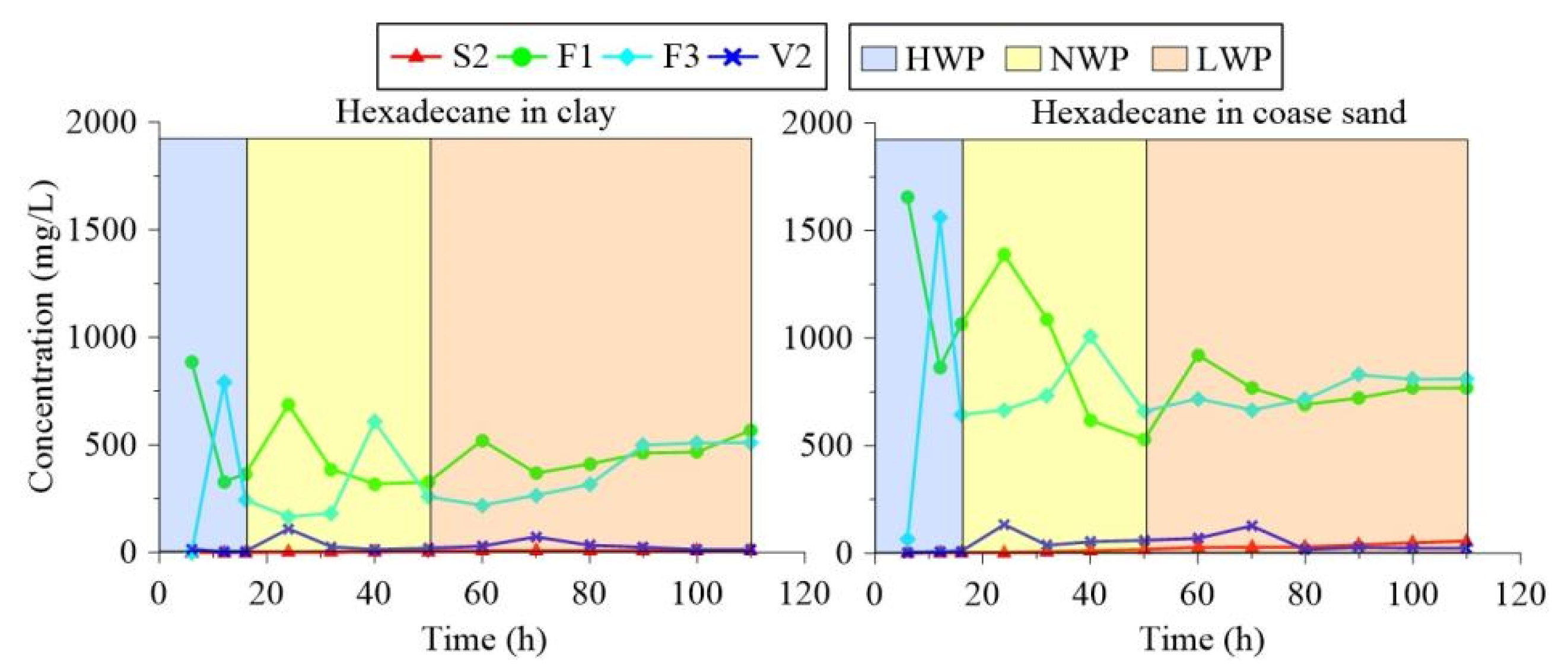
Water sampling: After 3 h, a water sample was collected from the lateral-face sampling hole. The sampling volume was 10 mL, and all sampling holes were accessible during sample collection. Whereas the samples from hole S2 represented the aquifer, samples F1 and F3 represented the water table fluctuation zone. According to the primary test and references [42], the sampling times were 6 h, 12 h, 16 h, 24 h, 32 h, 40 h, 50 h, 60 h, 70 h, 80 h, 90 h, 100 h, and 110 h.
(3)
Gas sampling: The majority of the gas samples were taken from the V2 hole in the aeration zone. The gas-sampling system was installed in the sampling hole. The injector was subsequently adopted. Sampling times were 6 h, 12 h, 16 h, 24 h, 32 h, 40 h, 50 h, 60 h, 70 h, 80 h, 90 h, 100 h, and 110 h.
After reprocessing the soil, water, and gas samples, the GC-MS was utilized to determine the concentration. The GC-MS test conditions were as follows: (1) Chromatographic conditions, using a capillary column (30 m × 0.25 mm × 0.25 μm). The gas chromatography inlet temperature was 250 °C, with split injection (split ratio 10:1). The carrier gas was high-purity helium (purity 99.999%). The current mode was constant, and column flow was 10 mL/min. The temperature-programming process was as follows: the initial column box was 35 °C, maintained for 3 min, then increased to 150 °C at 10 °C/min, maintained for 2 min, and then increased to 200 °C at 20 °C/min for 2 min. (2) Mass spectrometry conditions were as follows: electron multiplier voltage, 2108 eV; GC-MS interface temperature, 250 °C; ion source temperature, 230 °C; electron energy, 70 eV. The full scan mass range was 50~400 m/z.

3. Results and Discussion

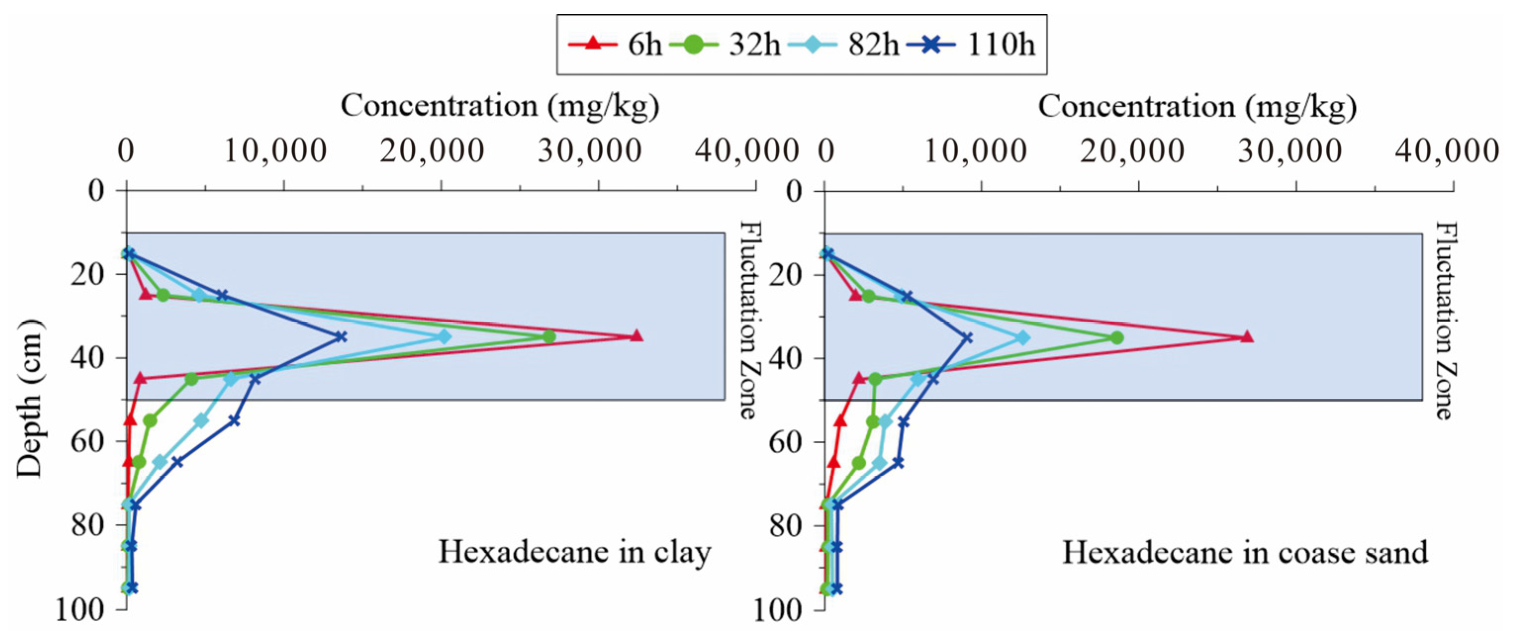
3.1. Change Rules of Chain Alkanes in the Water Fluctuation Process

The pollutants were separated into the water phase, the soil phase, and the gas phase, based on the migration status of their constituents, in order to investigate the migration rules and analyze the change process between the three parties. The chain alkanes constituted 60–90% of the total amount of petroleum, forming the primary component. Thus, the changing process largely reflected the migration law of the petroleum-dominated mixed pollutants.
Figure 8 depicts the changing rules of the water- and gas-phase concentrations of hexadecane during the fluctuations in the water table. Comparing the figures revealed the following: (1) The concentration of hexadecane in water was not high overall. The minimum value of the clay was 0.51 mg/L, and the maximum value was 883.82 mg/L. The lowest concentration of water in the coarse sand was 11.12 mg/L due to its high permeability, which was significantly greater than that of clay. Consequently, the soil medium had a significant effect on the fluctuations in component concentrations. Similarly, the average concentrations of hexadecane in the gas phase were 28.75 mg/L (clay) and 44.91 mg/L (coarse sand). (2) During the high-water period with rapid fluctuations, the sample concentration in each soil column was greater than that of the normal-water and low-water periods. In addition, the concentrations varied significantly, being 555.3 mg/L for clay and 791.3 mg/L for coarse sand, respectively. During periods of low water with slow fluctuations, the concentration was typically low. In the clay and coarse sand, the amplitudes of variation were 199.5 mg/L and 230.2 mg/L, respectively. The fluctuations in the water tables may have a significant effect on the concentration of pollutants in the water. (3) The changes were especially noticeable at different depths, and the concentrations in the saturated zone were quite low. Its average concentration was 4.52 mg/L in clay and 20.78 mg/L in coarse sand. The concentrations in F1 and F3 primarily reflected the fact that, when the water content was relatively high, its concentration increased proportionally, indicating that the pollutant component was carried in the water table fluctuations, thereby forming the free phase for migration. The concentration of the gas sample in the V2 hole indicated the volatility of the pollutants, as shown in the table. The volatility of hexadecane was very low and relatively low in clay and coarse sand.
The initial leakage position and the water table fluctuations had a combined effect on the component changes in the soil. As depicted in Figure 9, when the pollution components began to migrate upward with the water flow from their initial position, soil particles continuously adsorbed the pollution components. Consequently, the concentration in the soil rapidly increased, primarily at the site of the pollutant leak. Due to hexadecane’s high glutinousness, however, the viscosity in the saturated region was 3.34 mPa·s. After entering the soil prespace, this was readily absorbed by the soil or blocked as the residual phase during migration. Few quantities existed in the saturated zone. Despite the fact that water table fluctuations can transport hexadecane for migration, this was a minor factor. Therefore, the change in concentration in the vertical direction was not significant. Some pollutants may be transported for migration as a result of the fluctuation process, and their variation varied between fluctuation periods. After 6 h of hexadecane injection (high-frequency fluctuation period), the concentrations of clay and coarse sand at 40 cm (injecting position) were 32,425.8 mg/kg and 26,851.5 mg/kg, respectively, indicating that hexadecane in the coarse sand migrated to other positions within 6 h. Consequently, the concentration at other depths was relatively high in the coarse-sand fluctuation zone, which also enlarged the highly contaminated area. At this time, the concentration had the greatest change range, and the rate of change at 40 cm was 214.3 mg/(kg·h) for clay and 316.2 mg/(kg·h) for coarse sand. This was due to the fact that the substance carried due to water table fluctuations accelerated the migration in a short period, thereby shortening the contact time with the soil and decreasing the amount of content adsorbed by the soil. The free phase and dissolved phase migrated as the amount of water increased, resulting in a greater amount of material entering the saturated layer. A small amount of hexadecane migrated with water during low-frequency fluctuations, and the concentration in the saturated zone continued to maintain a stable, low-table trend. During the fluctuation period, the concentration of hexadecane changed at rates of 121.6 mg/(kg·h) and 170.1 mg/(kg·h) for clay and coarse sand at a depth of 40 cm, which was significantly slower than the rate of change that occurred during rapid water-table changes. Consequently, hexadecane may be absorbed by the low-permeability soil layer after leakage, and the pollution area continuously expanded due to the carrying effects of fluctuating water tables. The final contents that entered the aquifer were negligible, but the residual part entered sustainably, posing a long-term threat.

3.2. Change Rules of Cycloalkane in the Water Fluctuation Process

In comparison with hexadecane, the cycloalkane is an alkane with a relatively stable structure, resulting in a significant difference in its nature. (1) After entering the water solution, the lowest and highest concentrations of cyclohexane in migrated clay were 11.20 mg/L and 1386.50 mg/L, respectively. The lowest concentration in coarse-sand water samples was 13.68 mg/L, which was greater than the concentration in clay water. The glutinousness of cyclohexane was 0.98 mPa·s, which was relatively slow. The soil’s absorbency was relatively slow. As a result, the formed free phase had a strong ability to migrate, causing the concentration in the water to significantly fluctuate. (2) During the low-water period, when the fluctuation frequency was high, the amplitude of variation for concentration was 665.5 mg/L for clay and 703.9 mg/L for coarse sand. The concentration tended to be stable, and its amplitudes for clay and coarse sand were 246.8 mg/L and 362.6 mg/L, respectively. (3) In the saturated zone of the water solution, the average concentration of cyclohexane was 33.78 mg/L for clay and 43.49 mg/L for coarse sand. It was relatively stable, without any obvious fluctuations. F1 was a sampling point located above the fluctuation zone. The water’s concentration value significantly increased as the water table rose. The fluctuation zone’s lowest sampling point was F3. Compared to F1 and F3, the average concentrations in the aqueous phase were 725.88 mg/L and 624.51 mg/L (clay), and 858.56 mg/L and 659.25 mg/L (coarse sand). F1 had a higher concentration than F3. This indicated that the component density was less than that of water, so it flowed and migrated upwards, resulting in a higher concentration in the upper fluctuation zone than in the lower zone. Similarly, the average gas sample concentrations in the V2 hole were quite low, at 33.73 mg/L (clay) and 103.93 mg/L (coarse sand), with the concentration in coarse sand being slightly higher than that in clay, indicating that cyclohexane had low volatility and its concentration in the gas phase was relatively low (Figure 10).
After 6 h of injecting cyclohexane into the soil column, the concentration at the injection point was 24,621.8 mg/kg for clay and 18,089.6 mg/kg for coarse sand, which was significantly less than that of hexadecane. This indicated that less cyclohexane remained at the leakage position, and more cyclohexane had migrated to other positions in the free phase via water.
The change rates at 40 cm were 302.48 mg/(kg·h) and 345.23 mg/(kg·h) for clay and coarse sand during the high-water period with high-frequency fluctuations, which was significantly higher than that of hexadecane. This indicated that the migration of the cyclohexane in the free phase was strong, and it could have migrated to other locations from the pollution sources. Similarly, the components that migrated via low-frequency water table fluctuations were diminished, resulting in minor concentration changes in the saturated zone. The rates of concentration change for the two media at 40 cm were 99.32 mg/(kg·h) and 100.43 mg/(kg·h) (Figure 11).

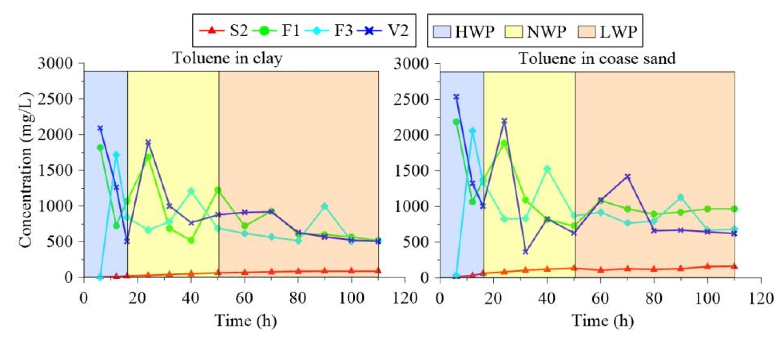
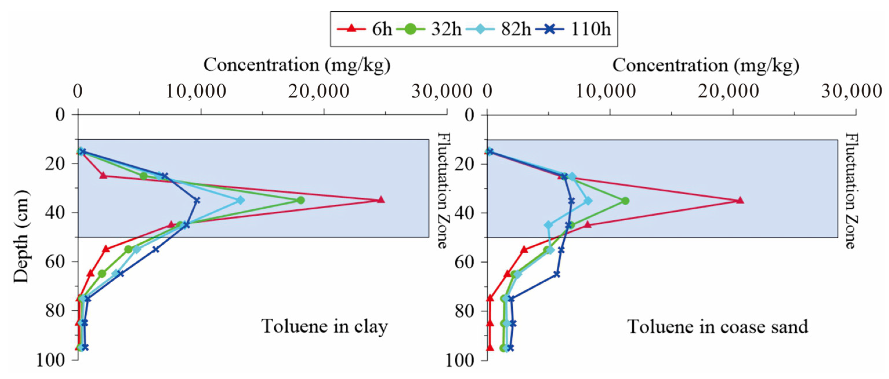
3.3. Change Rules of Aromatic Hydrocarbon in the Water Fluctuation Process

As a major component of petroleum and the most toxic substance to the human body, aromatic hydrocarbons have been the focus of domestic and international research. They exhibit high volatilization and solubility. When toluene migrated through clay, the minimum and maximum concentrations in the water solution were 13.20 mg/L and 1386.50 mg/L, respectively; for coarse sand, the corresponding values were 18.52 mg/L and 2185.8 mg/L. Toluene possessed a relatively weak viscosity of 0.59 mPa·s. Due to the relatively low absorbability of the soil, the free phase’s ability to migrate was increased. The maximum concentration in soil reached 24,621.8 mg/kg.
Due to its high volatility, toluene’s concentration in the gas phase was relatively high, with average values of 959.65 mg/L (clay) and 1076.73 mg/L (coarse sand). As shown in Figure 8, the concentration of toluene in the gas phase was similar to that in water, and its change rules were similar. The concentration increased as the amount of water increased. Toluene was carried up in large quantities as the water table rose because it floats on the water’s surface. Toluene was collected at the gas sampling point, so the concentration was high. Similarly, toluene had a higher concentration in water when the initial fluctuations were rapid, i.e., 1092.8 mg/L (clay) and 1121.3 mg/L (coarse sand). At a later stage, the fluctuation was slower, and the concentration change tended to stabilize. The amplitudes of variation were 317.0 mg/L (clay) and 355.2 mg/L (coarse sand). Toluene had a strong ability to migrate, and its concentration in the groundwater-saturated zone was quite high. The average values for clay and coarse sand were 56.82 mg/L and 104.86 mg/L, respectively (Figure 12).
After operating toluene for 6 h under fluctuating water tables, its concentrations of clay and coarse sand at the initial leakage location (40 cm) were 24,621.8 mg/kg and 20,581.5 mg/kg, respectively, with the least amount of residue among the four components. This indicated that, under the same conditions, the fluctuating water table could transport more toluene from the pollution source to other locations. During the fluctuation period, there was a substantial change in the concentration of toluene, and its concentration remained high throughout the entire fluctuation zone.
During the high-water period, the rates of change for clay and coarse sand were 251.23 mg/(kg·h) and 359.62 mg/(kg·h) at 40 cm, respectively. During the low-frequency fluctuations, the rates of concentration change were 108.0 mg/(kg·h) and 55.98 mg/(kg·h) at 40 cm for the two media. Toluene was distributed significantly differently to other soil constituents. Although they were concentrated at the initial position of leakage and formed the smear zone, they were continuously transported by the rise in water table fluctuations and could also form the gas phase for volatilization and diffusion. Thus, toluene was gradually distributed throughout the entire soil column section, and the concentration difference throughout the entire fluctuation zone was relatively small. The maximum difference in concentration was only 847.5 mg/kg (Figure 13).

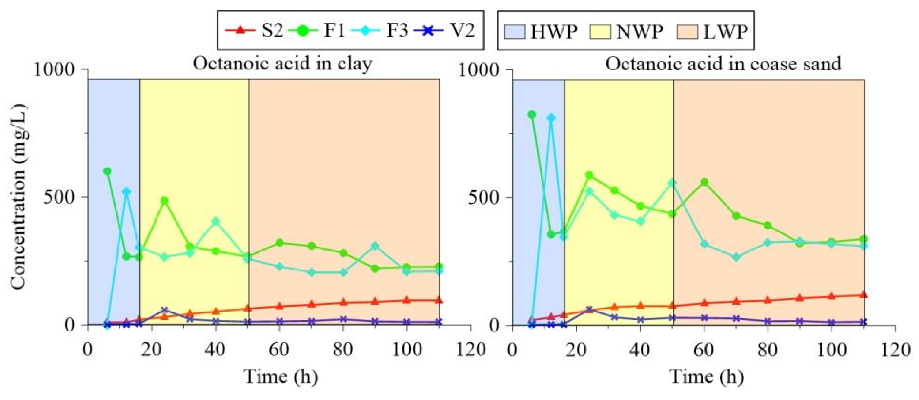
3.4. Change Rules of NOS Organic Substances in the Water Table Fluctuation Process

At the F1 sample hole in the fluctuation zone, the aqueous phase’s highest concentrations of octanoic acid were 602.3 mg/L (clay) and 825.8 mg/L (coarse sand). The average values were 313.39 mg/L (clay) and 456.52 mg/L (coarse sand). In the saturated zone, the concentration was relatively higher and exhibited an upward trend. At the S2 sample hole, the average concentrations were 2.68 mg/L (clay) and 4.45 mg/L (coarse sand); despite octanoic acid’s high solubility, its viscosity was high, making its migration difficult after forming the free phase. In addition, when it migrated vertically through the fluctuation zone, it was transferred to the residual phase and was difficult to dissolve due to the low water content. Consequently, the concentration was moderately low. As shown in Figure 10, the concentration in the soil column water sample was greater during the rapid fluctuations in the early period than during the normal-water and low-water periods. In addition, its amplitudes of variation were substantial, being 333.8 mg/L (clay) and 470.2 mg/L (coarse sand). In the later period, the amplitudes of variation decreased to 100.8 mg/L (clay) and 240.1 mg/L (coarse sand). The gas phase had the lowest concentration and the least amount of fluctuation. Its average values were 15.84 mg/L (clay) and 20.88 mg/L (coarse sand), again demonstrating octanoic acid’s low volatility (Figure 14).
Compared to the aqueous phase, soil particles readily adsorbed octanoic acid, primarily due to their high glutinousness (5.83 mPa·s). After the octanoic acid was injected for 6 h, the octanoic acid concentrations in the clay and coarse sand at a site 40 cm from the injection point were 36,051.8 mg/kg and 33,122.2 mg/kg, respectively. This indicated that the octanoic acid was primarily maintained at the initial leakage position, and only slowly migrated by diffusion. At the pollution leakage location, the concentration was consistently the highest, with an average value of 23,290.4 mg/kg. However, its concentration at other depths was typically low (Figure 15). Due to the high-frequency fluctuations during the high-water period, the amplitude of variation for octanoic acid concentration was relatively small. The rates of change were 199.89 mg/(kg·h) and 319.27 mg/(kg·h) for clay and coarse sand at 40 cm. At the low-frequency fluctuation, the portion that was carried and migrated was less, and the saturated zone always showed a gentle trend and was maintained within a low concentration range. For two media, the rates of concentration change were 117.81 mg/(kg·h) and 189.61 mg/(kg·h), which were significantly less than when the water table fluctuates quickly.

3.5. Instructions for Remediation Strategy

Due to the complexity of groundwater pollution remediation and the differences between contaminated site conditions, the remediation of contaminated groundwater and its scientific and engineering problems are becoming challenges for research in related fields. Although many studies on the petroleum pollution of groundwater have been carried out, the research results mainly focus on pollution sources, pollution pathways, pollution mechanisms, and pollution forecasting. An effective treatment technology and remediation engineering practices at actual contaminated sites have not been shown.
Based on the experimental conclusions obtained in this study, it can be seen that, due to the differences in component properties and soil–groundwater characteristics of petroleum pollutants (especially soil types and water table fluctuations), once pollutants entered the underground environment, they showed very complex migration and transformation rules. Some pollutants can exist in the environment for decades, posing a continuous threat to the surrounding humans and the environment. This was also the root cause of the difficulties in oil pollution remediation. Specifically, although there are many oil-pollution control technologies, such as AS, SVE, PRB, and P&T, these technologies have certain limitations, and some can only be used for a specific type of pollutant. Obtaining a single technology that can be used to completely control oil pollution appeared to be basically impossible. The results of this study can help to guide comprehensive treatments via different technologies.
As shown in Figure 16, according to the experimental conclusions, there are many volatile components (such as toluene) in the vadose zone, and the characteristics of AS were just to remove volatile organic compounds. Therefore, AS equipment can be set up in the vadose zone. More specifically, the AS technique can be applied to areas where volatile, semivolatile, and biodegradable nonvolatile organic compounds cause groundwater and saturated soil pollution and can also be applied to areas where dehydration (gas extraction in residual contaminated soil) is not feasible, including high aquifers and thick smear zones (mainly residual and free components). In practical applications, the AS technique is often used in combination with the SVE technique, based on the characteristics of the volatile phase, to exert a greater removal effect.
Similarly, in the water table fluctuation zone, repeated water flushing will dissolve a large number of dissolved pollutants and carry out free pollutants, so the P&T technique can be used to remove the dissolved and free-phase pollutants from the water. In addition, permeable reactive barrier (PRB) refers to a wall with reactive materials set in the flow path of groundwater. When pollutants flow through the reactive wall, a series of physical, chemical, and biological effects, such as adsorption, redox, and degradation, occur with the materials in the wall. The pollution components are converted into nontoxic components or are retained in the wall to achieve the purpose of groundwater remediation. At the actual polluted site, the PRB technique involves setting the PRB in the direction of groundwater flow so that it can control a large number of free-phase components moving with the water flow. Specifically, excavation is conducted along the direction of the groundwater flow at the petroleum pollution leakage point, and then the PRB device is installed and fixed, which can greatly retain and degrade the pollutants flowing with the groundwater. Hence, the results of this study provided a specific and targeted comprehensive strategy for petroleum pollution treatment.

4. Conclusions

In this study, column experiments with homogenous soil media (coarse sand and clay) were conducted to research the vertical transportation of different types of petroleum contaminants under groundwater table fluctuations. The findings indicated the following: (1) Due to the influence of composition and soil media characteristics, the vertical transportations of four components were different. The differences in the components came from viscosity, volatility, and solubility. More specifically, toluene had lower viscosity and stronger volatility, so the concentration of the residual phase was the smallest. In contrast, hexadecane and octanoic acid had higher viscosities and tended to be adsorbed by soil, and the dissolved phase of hexadecane showed only a small change. The concentrations of the residual phase were octanoic acid > hexadecane > cyclohexane > toluene. The soil media differences were reflected in the influence of the soil characteristics. Compared to clay, coarse sand had more soil particles, a lower clay content, and a smaller specific surface area, which represented its weak adsorption capacity. Therefore, the migration pattern of the components in coarse sand was a convective rapid influx. In contrast, the components can be largely retained in clay due to its strong adsorption capacity. (2) There were two obvious pollution accumulation zones under the condition of water table fluctuations: (i) the pollution infiltration zone dominated by the residual phase was formed at the leakage position, and (ii) the floating zone dominated by the free phase was formed near the water table. (3) Different fluctuation frequencies had a great influence on the migration process of components. When the fluctuation frequency was low, the pollutants could migrate slowly, and the interactions with soil, water, and gas were very frequent; hence, the soil could fully adsorb the free phase into the residual phase. In the case of high-frequency groundwater fluctuations, there were more free phase components that could be carried by the water flow. (4) According to the experimental conclusions, the types of petroleum pollution components were very complex in the soil and groundwater system (especially in the case of groundwater fluctuations), which formed three phases (free phase, dissolved phase, and residual phase). These three phases of pollutants all converted into each other, which was the root cause of the difficulty in repairing petroleum pollution. Therefore, in the project of petroleum pollution control, it is necessary to adopt different remediation techniques (for example, AS, PRB, P&T, and SVE) at different stages of pollution components, according to the pollution components and environmental characteristics, so as to achieve cost-effective treatment effects.

Author Contributions

Conceptualization, M.Y.; formal analysis, Z.C. and T.T.; funding acquisition, M.Y.; methodology, M.Y. and Z.C.; resources, X.S.; software, T.T. and X.S.; supervision, M.Y.; writing—original draft preparation, Z.C. All authors have read and agreed to the published version of the manuscript.

Funding

This research was sponsored by the Geology Science and Technology Project of the Guizhou Bureau of Geology and Mineral Exploration and Development (QDKKH(2016)-21); the Guizhou Provincial Science and Technology Projects (QKHJC-ZK(2022)—General 186); Projects of the National Natural Science Foundation of China (No. 41602275, 41977298); and the Provincial Key Disciplines of Guizhou Province—Geological Resources and Geological Engineering (ZDXK (2018)001).

Institutional Review Board Statement

Not applicable.

Informed Consent Statement

Not applicable.

Data Availability Statement

Data sharing is not applicable to this article.

Conflicts of Interest

The authors declare no conflict of interest.

References

  1. Bajagain, R.; Jeong, S.W. Degradation of petroleum hydrocarbons in soil via advanced oxidation process using peroxymonosulfate activated by nanoscale zero-valent iron. Chemosphere 2021, 270, 128627. [Google Scholar] [CrossRef] [PubMed]
  2. Yang, Z.H.; Verpoort, F.; Dong, C.D.; Chen, C.W.; Chen, S.; Kao, C.M. Remediation of petroleum-hydrocarbon contaminated groundwater using optimized in situ chemical oxidation system: Batch and column studies. Process. Saf. Environ. 2020, 138, 18–26. [Google Scholar] [CrossRef]
  3. Atlas, R.M.; Hazen, T.C. Oil biodegradation and bioremediation: A tale of the two worst spills in US history. Environ. Sci. Technol. 2011, 45, 6709–6715. [Google Scholar] [CrossRef] [Green Version]
  4. Yao, Y.; Mao, F.; Xiao, Y.; Luo, L. Modeling capillary fringe effect on petroleum vapor intrusion from groundwater contamination. Water Res. 2019, 150, 111–119. [Google Scholar] [CrossRef] [PubMed]
  5. Zhang, Q.; Wang, G.; Sugiura, N.; Utsumi, M.; Zhang, Z.; Yang, Y. Distribution of petroleum hydrocarbons in soils and the underlying unsaturated subsurface at an abandoned petrochemical site, North China. Hydrol. Process. 2014, 28, 2185–2191. [Google Scholar] [CrossRef]
  6. Chandra, S.; Sharma, R.; Singh, K.; Sharma, A. Application of bioremediation technology in the environment contaminated with petroleum hydrocarbon. Ann. Microbiol. 2013, 63, 417–431. [Google Scholar] [CrossRef]
  7. Bolade, O.P.; Adeniyi, K.O.; Williams, A.B.; Benson, N.U. Remediation and optimization of petroleum hydrocarbons degradation in contaminated water using alkaline activated persulphate. J. Environ. Chem. Eng. 2021, 9, 105801. [Google Scholar] [CrossRef]
  8. Xia, C.; Liu, Q.; Zhao, L.; Wang, L.; Tang, J. Enhanced degradation of petroleum hydrocarbons in soil by FeS@BC activated persulfate and its mechanism. Sep. Purif. Technol. 2022, 282, 120060. [Google Scholar] [CrossRef]
  9. Liu, B.; Liu, F.; Chen, H. Sorption characteristics of the major components of crude oil to vadose zone soil in Xinjiang oilfield, China. Fresenius Environ. Bull. 2013, 22, 3–10. [Google Scholar]
  10. Liu, J.; Wei, K.; Xu, S.; Cui, J.; Ma, J.; Xiao, X.; Xi, B.; He, X. Surfactant-enhanced remediation of oil-contaminated soil and groundwater: A review. Sci. Total Environ. 2021, 756, 144142. [Google Scholar] [CrossRef]
  11. Li, K.; Ding, W.; Wang, F.; Lu, Z.; Chen, Y. Countermeasure and suggestions for soil contamination prevention and control of oil exploration industry. Environ. Prot. Chem. Ind. 2019, 39, 603–607. (In Chinese) [Google Scholar]
  12. Wang, B.; Liu, Q.; Zhang, S.; You, H.; Ma, Y.; An, J. Adsorption of petroleum pollutants released from soil by biocha. Acta Pet. Sin. Pet. Process. Sect. 2019, 35, 603–612. (In Chinese) [Google Scholar]
  13. Li, J.; Cao, X.; Sui, H.; He, L.; Li, X. Research status and prospect of petroleum contaminated soil remediation technology. Acta Pet. Sin. Pet. Process. Sect. 2017, 33, 811–833. (In Chinese) [Google Scholar]
  14. API. Technical Data Book-Petroleum Refining, 5th ed.; American Petroleum Institute: Washington, DC, USA, 1992. [Google Scholar]
  15. Song, D.; Kitamura, M.; Katayama, A.A. Approach for estimating microbial growth and biodegradation of hydrocarbon contaminants in subsoil based on field measurements: 2. Application in a field lysimeter experiment. Environ. Sci. Technol. 2010, 44, 6795–6801. [Google Scholar] [CrossRef]
  16. Ding, A.; Liu, B.; Liang, X.; Li, S.; Zhang, L.; Yin, H. A review of the petroleum hydrocarbon contamination transformation performance in the zone of intermittent saturation. Sci. Technol. Eng. 2018, 18, 172–178. (In Chinese) [Google Scholar]
  17. Podgorski, D.C.; Zito, P.; Kellerman, A.M.; Bekins, B.A.; Spencer, R.G.M. Hydrocarbons to carboxyl-rich alicyclic molecules: A continuum model to describe biodegradation of petroleum-derived dissolved organic matter in contaminated groundwater plumes. Environ. Technol. Innov. 2018, 10, 175–193. [Google Scholar] [CrossRef]
  18. Abbas, O.; Rebufa, C.; Dupuy, N.; Permanyer, A.; Kister, J. Assessing petroleum oils biodegradation by chemometric analysis of spectroscopic data. Talanta 2008, 75, 857–871. [Google Scholar] [CrossRef]
  19. Rayner, J.L.; Snape, I.; Walworth, J.L.; Harvey, P.; Ferguson, S.H. Petroleum–hydrocarbon contamination and remediation by microbioventing at sub-Antarctic Macquarie Island. Cold Reg. Sci. Technol. 2015, 48, 139–153. [Google Scholar] [CrossRef]
  20. Weishaar, J.A.; Tsao, D.; Burken, J.G. Phytoremediation of BTEX hydrocarbons: Potential impacts of diurnal groundwater fluctuation on microbial degradation. Int. J. Phytoremediat. 2009, 11, 509–523. [Google Scholar] [CrossRef]
  21. Lenhard, R.J.; Oostrom, M.; Dane, J.H. A constitutive model for air-NAPL-water flow in the vadose zone accounting for immobile, non-occluded (residual) NAPL in strongly water-wet porous media. J. Contam. Hydrol. 2004, 71, 261–282. [Google Scholar] [CrossRef]
  22. Oostrom, M.; Hofstee, C.; Lenhard, R.J.; Wietsma, T.W. Flow behavior and residual saturation formation of liquid carbon tetrachloride in unsaturated heterogeneous porous media. Contam. Hydrol. 2003, 4, 163–174. [Google Scholar] [CrossRef] [PubMed]
  23. Jarsjö, J.; Destouni, G.; Yaron, B. Retention and volatilisation of kerosene: Laboratory experiments on glacial and post-glacial soils. J. Contam. Hydrol. 1994, 17, 167–185. [Google Scholar] [CrossRef]
  24. Atekwana, E.A.; Atekwana, E.A. Geophysical signatures of microbial activity at hydrocarbon contaminated sites: A review. Surv. Geophys. 2010, 31, 247–283. [Google Scholar] [CrossRef]
  25. Bekins, B.A.; Cozzarelli, I.M.; Godsy, E.M.; Warren, E.; Essaid, H.I.; Tuccillo, M.E. Progression of natural attenuation processes at a crude oil spill site: II. Controls on spatial distribution of microbial populations. J. Contam. Hydrol. 2001, 53, 387–406. [Google Scholar] [CrossRef] [PubMed]
  26. Rijal, M.L.; Appel, E.; Petrovský, E.; Blaha, U. Change of magnetic properties due to fluctuations of hydrocarbon contaminated groundwater in unconsolidated sediments. Environ. Pollut. 2010, 158, 1756–1762. [Google Scholar] [CrossRef]
  27. McCray, J.E.; Tick, G.R.; Jawitz, J.W.; Gierke, J.; Brusseau, M.; Falta, R.; Knox, R.; Sabatini, D.; Annable, M.; Harwell, J.; et al. Remediation of NAPL source zones: Lessons learned from field studies at Hill and Dover AFB. Groundwater 2011, 49, 727–744. [Google Scholar] [CrossRef] [Green Version]
  28. Tzovolou, D.N.; Benoit, Y.; Haeseler, F.; Klintd, K.E.; Tsakiroglou, C.D. Spatial distribution of jet fuel in the vadoze zone of a heterogeneous and fractured soil. Sci. Total Environ. 2009, 407, 3044–3054. [Google Scholar] [CrossRef]
  29. Giampaolo, V.; Rizzo, E.; Titov, K.; Konosavsky, P.; Laletina, D.; Maineult, A.; Lapenna, V. Self-potential monitoring of a crude oil-contaminated site (Trecate, Italy). Environ. Sci. Pollut. Res. 2014, 21, 8932–8947. [Google Scholar] [CrossRef]
  30. Yang, M.; Yang, Y.S.; Du, X.; Cao, Y.; Lei, Y. Fate and Transport of Petroleum Hydrocarbons in Vadose Zone: Compound-specific Natural Attenuation. Water Air Soil Pollut. 2013, 224, 1439. [Google Scholar] [CrossRef]
  31. Lopes de Castro, D.; Branco, R.M.G.C. 4-D ground penetrating radar monitoring of a hydrocarbon leakage site in Fortaleza (Brazil) during its remediation process: A case history. J. Appl. Geophy. 2003, 54, 127–144. [Google Scholar] [CrossRef]
  32. Thorstad, J.L. Influence of Borehole Construction on LNAPL Thickness Measurements; Oklahoma State University: Stillwater, OK, USA, 2007. [Google Scholar]
  33. Vermaak, K.H. Characterisation and Management of a LNAPL Pollution Site along the Coastal Regions; University of the Free State: Bloemfontein, South Africa, 2009. [Google Scholar]
  34. Luo, J.; Lu, W.; Yang, Q.; Ji, Y.; Xin, X. An adaptive dynamic surrogate model using a constrained trust region algorithm: Application to DNAPL-contaminated-groundwater-remediation design. Hydrogeol. J. 2020, 28, 1285–1298. [Google Scholar] [CrossRef]
  35. Villaume, J.F. Investigations at Sites Contaminated with Dense, Non-Aqueous Phase Liquids (NAPLs). Groundw. Monit. R. 2010, 5, 60–74. [Google Scholar] [CrossRef]
  36. Shi, J.; Deng, F.; Xiao, L.; Liu, H.; Ma, F.; Wang, M.; Zhao, R.; Chen, S.; Zhang, J.; Xiong, C. A proposed NMR solution for multi-phase flow fluid detection. Pet. Sci. 2019, 16, 212–222. [Google Scholar] [CrossRef] [Green Version]
  37. Gudbjerg, J.; Sonnenborg, T.O.; Jensen, K.H. Remediation of NAPL below the water table by steam-induced heat conduction. J. Contam. Hydrol. 2004, 72, 207–225. [Google Scholar] [CrossRef]
  38. Ossai, I.C.; Ahmed, A.; Hassan, A.; Hamid, F.S. Remediation of soil and water contaminated with petroleum hydrocarbon: A review. Environ. Technol. Innov. 2020, 266, 100526. [Google Scholar] [CrossRef]
  39. Marcon, L.; Oliveras, J.; Puntes, V.F. In situ nanoremediation of soils and groundwaters from the nanoparticle’s standpoint: A review. Sci. Total. Environ. 2021, 791, 148324. [Google Scholar] [CrossRef]
  40. Balseiro-Romero, M.; Monterroso, C.; Casares, J.J. Environmental Fate of Petroleum Hydrocarbons in Soil: Review of Multiphase Transport, Mass Transfer, and Natural Attenuation Processes. Pedosphere 2018, 28, 3–17. [Google Scholar] [CrossRef]
  41. Oostrom, M.; Hofstee, C.; Wietsma, T.W. LNAPLs do not Always Float: An Example Case of a Viscous LNAPL under Variable Water Table Conditions. J. Hydrol. Days 2006. [CrossRef]
  42. Miller, C.D.; Durnford, D.S.; Fowler, A.B. Equilibrium nonaqueous phase liquid pool geometry in coarse soils with discrete textural interfaces. J. Contam. Hydrol. 2004, 71, 239–260. [Google Scholar] [CrossRef]
  43. Roy, J.W.; Smith, J.E. Multiphase flow and transport caused by spontaneous gas phase growth in the presence of dense non-aqueous phase liquid. J. Contam. Hydrol. 2007, 89, 251–269. [Google Scholar] [CrossRef]
  44. Zhen, X.L.; Wang, B.C.; She, Z.L. Principle and Application of Oil Pollution in Soil—Groundwater System; Geological Publishing House: Beijing, China, 2004. (In Chinese) [Google Scholar]
Figure 1. Conceptual model of the transportation of NAPL pollutants in the groundwater and soil system.
Sustainability 15 06514 g001
Figure 2. Types of pollutants in the contaminated oilfield [30]. TPH: total petroleum hydrocarbons; Chs: chainalkane hydrocarbons; Cys: cycloalkane hydrocarbons; Ars: aromatic hydrocarbons; Aps: asphaltenes hydrocarbons.
Sustainability 15 06514 g002
Figure 3. A profile map of shallow aquifer in the contaminated oilfield.
Sustainability 15 06514 g003
Figure 4. Grain size distribution of the experimental soil media.
Sustainability 15 06514 g004
Figure 5. One-dimensional homogeneous media column experimental device. (V (red), F (green), and S (yellow) indicate sampling sites for volatilization, fluctuation, and saturation areas).
Sustainability 15 06514 g005
Figure 6. Water table fluctuations in bore hole 1 of the contaminated oilfield.
Sustainability 15 06514 g006
Figure 7. Water table fluctuation process at different frequencies. HWP, NWP, and LWP indicate high-water period, normal-water period, and low-water period, respectively.
Sustainability 15 06514 g007
Figure 8. The concentration-change process of hexadecane in water and gas phases in different soil media under different fluctuation conditions (HWP, MWP, and LWP mean high-, normal-, and low-water periods).
Sustainability 15 06514 g008
Figure 9. The concentration-change process of hexadecane in the soil phase in different soil media under different fluctuation conditions.
Sustainability 15 06514 g009
Figure 10. The concentration-change process of cyclohexane in the water and gas phases in different soil media under different fluctuation conditions (HWP, MWP, and LWP mean high-, normal-, and low-water periods).
Sustainability 15 06514 g010
Figure 11. The concentration-change process of cyclohexane in the soil phase in different soil media under different fluctuation conditions.
Sustainability 15 06514 g011
Figure 12. The concentration-change process of toluene in water and gas phases in different soil media under different fluctuation conditions (HWP, MWP, and LWP mean high-, normal-, and low-water periods).
Sustainability 15 06514 g012
Figure 13. The concentration-change process of toluene in the soil phase in different soil media under different fluctuation conditions.
Sustainability 15 06514 g013
Figure 14. The concentration-change process of octanoic acid in water and gas phase in different soil media under different fluctuation conditions (HWP, MWP, and LWP mean high-, normal-. and low-water periods).
Sustainability 15 06514 g014
Figure 15. The concentration-change process of octanoic acid in the soil phase in different soil media under different fluctuation conditions.
Sustainability 15 06514 g015
Figure 16. Comprehensive remediation strategy based on the vertical transportation of petroleum pollutants.
Sustainability 15 06514 g016
Table 1. Soil media and water fluctuation amplitudes of different oil contaminated sites of different countries.
PSPSM & D (m)WFA
(m)
C
(g/kg)
R
Perth (Australia)Diesel oilmixture of fine, medium and coarse sand (4)0.840.1[23]
Crystal Refinery (Mexico)Crude oilmedium sand (3.9), coarse sand (0.4), sandy gravel (0.6)0.3936.5[24]
Bemidji (USA)Crude oilmedium sand (5.0)0.37112.6[25]
Hradcany AFB (USA)Gasolinemixture of fine, medium and coarse sand (8)0.33316.9[26]
Northern Refinery (China)Crude oilloam (1.7–3), clay (5), mixture of fine, medium and coarse sand (4)2.056.3[5]
AFB (USA)Crude oilmixture of fine, medium and coarse sand (9)289.6[27]
Kluczewo (Poland)Gasolinesandy clay (1.7), medium sand (3.4), clay (1.9)0.5–1.068.6[28]
Trecate (Italy)Crude oilsilt (2.5), fine sand (7.5), clay (0.8), medium sand (5.0), sandy gravel (5.2)6.0125.8[29]
Northeastern oilfield (China)Crude oilfine sand (1.5), caly (1.5), medium sand (3.0), coarse sand (4.0)0.550.8[30]
Fortakeza (Brazil)Crude oilclay (2.3)1.8299.1[31]
Golden Oklahoma (USA)Crude oilsilt clay (4.6), sandy gravel (0.31), coarse sand (0.15)1.3–2.8121.2[32]
East London (England)Crude oilmedium sand (4), sandy clay (7)0.3–339.6[33]
PS = Pollution sites; P = Pollutants; SM & D = Soil Media and the Depth; WFA = Water Fluctuation Amplitude; C = Concentration; R = References.
Table 2. Properties of the petroleum compounds.
MW
(g/mol)
FGA
(cm−1)
S
(mg/L)
ρ
(g/cm3)
BP
(℃)
η
(mPa·s)
H
(cm3/cm3)
Log
Kow
Koc
(cm3/g)
Dair
(cm2/s)
Dwater
(cm2/s)
Hexadecane226.4-(CH2)n-2960260.7732873.341.6 × 1028.248.47 × 1060.0374.2 × 10−6
Cyclohexane84.2Sustainability 15 06514 i0011450550.77980.70.987.8 × 1003.449.63 × 1020.0849.1 × 10−6
Toluene92.1Sustainability 15 06514 i0027485150.866110.60.592.7 × 10−12.692.34 × 1020.0878.6 × 10−6
Octanoic acid144.2-COOH12446800.911239.75.835.0× 1023.051.10 × 1040.0233.6 × 10−6
MW = molar mass; S = solubility; ρ = density; BP = vapor pressure; η = viscosity; H = Henry’s constant; Kow = partition coefficient of n-octanoic alcohol; Koc = partition coefficient of organic carbon; Dair = dispersion coefficient in gas; Dwater = dispersion coefficient in water; FG = characteristic functional group; A = absorption wave number.
Table 3. Characteristics of the column media.
CharacteristicsColumn 1Column 2
Media typeCoarse sandClay
Packing weight (kg)12.9410.75
Packing height (cm)9090
Packing density (g/cm3)1.831.52
Porosity (%)30.942.7
Specific surface area (m2/kg)58.8449.6
Organic matter content (%)1.53.8
Mean diameter (μm)653.5545.53
Disclaimer/Publisher’s Note: The statements, opinions and data contained in all publications are solely those of the individual author(s) and contributor(s) and not of MDPI and/or the editor(s). MDPI and/or the editor(s) disclaim responsibility for any injury to people or property resulting from any ideas, methods, instructions or products referred to in the content.

