Article

Analysis of Detailed Lake Variations and Associated Hydrologic Driving Factors in a Semi-Arid Ungauged Closed Watershed

1
School of Water and Environment, Chang’an University, Xi’an 710054, China
2
Key Laboratory of Subsurface Hydrology and Ecological Effects in Arid Region, Ministry of Education, Chang’an University, Xi’an 710054, China
3
Faculty of Geosciences and Environmental Engineering, Southwest Jiaotong University, Chengdu 611756, China
4
Yantai Institute of Coastal Zone Research, Chinese Academy of Sciences, Yantai 264003, China
5
Ordos Forestry and Grassland Bureau, Ordos 017000, China
*
Authors to whom correspondence should be addressed.
Sustainability 2023, 15(8), 6535; https://doi.org/10.3390/su15086535
Submission received: 10 February 2023 / Revised: 30 March 2023 / Accepted: 1 April 2023 / Published: 12 April 2023

Abstract

:
Lakes are key factors in maintaining ecosystems in semi-arid regions. However, due to data shortage, most studies used remote-sensing data and water-balance models to analyze lake variations in semi-arid ungauged closed watersheds, resulting in the oversimplified assessment of lake variations and their associated hydrologic processes. This study aimed to enhance the understanding of the mechanisms behind the water supplement and consumption of lakes and reveal the influences of hydrological processes on lake variations in such watersheds. Physically based and lake-oriented hydrologic modeling, remote-sensing technology, and results from previous studies were comprehensively integrated to achieve the research objective. The Hongjiannao (HJN) watershed in Northwest China was selected as the study area of this research. The calibration and validation results demonstrated that remote-sensing data and results from previous studies indeed guaranteed the accuracy of the lake-oriented model. Further hydrologic and statistical analyses revealed the linkage between lake variations and their associated hydrologic processes, and the mechanisms behind the linkage. Specifically, rainfall and snowmelt were found to be the most stable sources of HJN Lake, particularly in dry years. Due to the differences in recession rates, groundwater inflow was more stable than upstream inflow and inflow from the contributing area of HJN Lake. The correlations between hydrologic processes and the storage variation of HJN Lake varied significantly at daily and monthly time scales, which can be explained by the generation mechanisms of these processes. This study provided valuable guidance for water resources management and ecosystem protection in the HJN watershed and can be further applied for hydrologic simulations in other similar watersheds.

1. Introduction

Lakes are essential elements for conserving water sources, purifying water quality, regulating ecological environments, and protecting biodiversity in semi-arid regions [1,2,3,4]. Due to low precipitation and intense evaporation, lakes in such regions are sensitive to environmental changes, and recovery from damage is difficult [5,6,7]. Over the past few decades, climate warming and human activities have significantly affected the water supplement and consumption of lakes in semi-arid regions, resulting in the shrinkage or disappearance of lakes, increased salinization, and changes in local ecosystems [8,9,10]. Therefore, it is crucial to understand the variations of lakes and the impacts of hydrologic processes on the variations to maintain the states of lakes and protect the fragile ecological environment in semi-arid regions [11,12].
Remote-sensing datasets, such as Landsat and MODIS data, have been widely used to extract lake areas and monitor the spatio-temporal variations of lakes [13,14,15]. Furthermore, the extracted lake areas can be combined with meteorological data (e.g., precipitation, temperature, and evaporation) to reveal the climatic driving factors of lake variations by using statistical methods [16,17,18]. Though the development of remote-sensing technology has improved data availability for natural scientific research in large-scale regions [19,20,21,22], the quality and quantity of the data are highly susceptible to climate conditions and record frequency [23,24]. Therefore, using only remote-sensing data may not be sufficient to obtain continuous daily variations of lakes and reveal the hydrological processes associated with the variations.
Integrating remote-sensing data with hydrologic modeling is an effective method to simulate and predict continuous hydrologic processes under various climate conditions [25,26,27]. Compared with remote-sensing data alone, the combined method can depict the internal hydrologic processes between climate and lakes (e.g., surface runoff, groundwater flow, and snowmelt), and quantify the impacts of these processes on lake variations [28,29,30]. Many studies have been conducted to simulate the daily variations of lakes and their associated hydrologic processes with long time periods in gauged watersheds [31,32,33]. However, due to the lack of observed streamflow, most studies in semi-arid and ungauged watersheds utilized simple water-balance models to simulate the water budgets and lake areas and analyze the hydrologic driving factors of lake variations at monthly or annual time scales [34,35,36,37]. These models cannot reveal detailed water-exchange procedures due to their simplified structures and large simulation time scales [38,39]. Therefore, studies using physically based hydrologic models with fine time scales are essential for promoting the simulation qualities in semi-arid and ungauged lake watersheds.
The selection of model evaluation data is critical for applying physically based models in semi-arid and ungauged watersheds. In some gauged watersheds, observed streamflow data and remotely sensed data have been utilized for model calibration and validation [40,41,42], and their combination indeed improved the performance of hydrologic models. For ungauged watersheds, several studies have verified the possibilities of using remote-sensing data (e.g., evapotranspiration, leaf area index, and soil moisture data) for model evaluation [43,44], and their results demonstrated that, without observed streamflow, the model calibrated by remotely sensed data can still simulate hydrologic processes appropriately. Overall, the above studies provide a feasible option for the evaluation of hydrologic models in data-poor watersheds and make the applications of the physically based models to semi-arid and ungauged closed watersheds possible.
The objective of this study was to establish a comprehensive approach to promote the understanding of lake supplement and consumption mechanisms and reveal the influences of hydrological processes on lake variations in semi-arid ungauged closed watersheds. Unlike previous studies that used simple water-balance models, the new approach adopted a modified lake-oriented hydrologic model to simulate hydrologic processes related to lake variations in closed watersheds, and utilized multiple remote-sensed data and results from previous studies to set up and evaluate the model. The new approach was further applied to the Hongjiannao (HJN) watershed in Northwest China, where there are no meteorological and stream gauge stations, to: (1) simulate detailed lake variations and their associated hydrologic processes with limited data; (2) reveal the linkage between lake variations and hydrologic processes at different time scales; and (3) interpret the linkage based on the generation mechanisms of lake-related hydrologic processes.

2. Materials and Methods

2.1. Study Area

HJN Lake is an irregular triangle-shaped lake that is located at the junction of Shaanxi and Inner Mongolia provinces in Northwest China. It is the largest freshwater desert lake in China and the largest habitat and breeding ground for relict gulls globally [45,46]. The lake was formed in 1929 with an area of 1.3 km2, which expanded to 60–67 km2 during the 1960–1970s and gradually decreased to 35 km2 in 2018 [45,46]. Currently, the east-west width, north-south length, and depth of HJN Lake are approximately 8 km, 11.2 km, and 8.2 m, respectively [45]. Before 2000, HJN Lake was supplied by seven seasonal rivers, which were the Zhasake River, Manggaitu River, Qibosu River, Mudushili River, Erlintu River, Songdaogou River, and Miaohao River [46] (Figure 1a). However, due to climate change and human activities, the Miaohao River, Erlintu River, and Songdaogou River have stopped supplying water to HJN Lake. Furthermore, in 2005, the construction of the Zhasake reservoir blocked the upstream section of the Zhasake River. Our field survey indicates that, in recent years, the Manggaitu River and Qibosu River have streamflow during dry periods, while the Zhasake River and Mudushili River have streamflow after rainfall events.
The HJN watershed is a closed lake watershed with a total area of 1343.79 km2, and an altitude of 1210 to 1518 m. There are no meteorological and hydrological stations in the watershed. Based on the record data of nearby meteorological stations, the HJN watershed receives most of the precipitation in summer, with annual precipitation ranging from 108.6 mm to 819.1 mm and annual temperature ranging from −28.1 ℃ to 38.9 ℃. In this study, ArcGIS Pro 2.8 and a surface delineation algorithm, HUD-DC [47], were used to identify rivers, HJN Lake, the Zhasake reservoir, and the boundaries of each sub-basin (Figure 1b) based on the ALOS Global Digital Surface Model (https://www.eorc.jaxa.jp/ALOS/en/dataset/aw3d30/aw3d30_e.htm (accessed on 16 May 2022)).

2.2. Research Approach

To accurately simulate the hydrologic processes and variations of HJN Lake, it is necessary to select a physically based model suitable for simulating the drainage from multiple rivers to a lake. The selected model should be able to simulate traditional hydrologic processes (e.g., surface runoff and runoff routing), and the variations of lakes and the hydrologic processes directly related to the lakes (e.g., lake evaporation and inflows from rivers and groundwater). Additionally, the model must be set up and evaluated based on limited available data. Input data of the model include meteorological data, land surface data, soil data, and groundwater data, which can be obtained from remote-sensing datasets and previous studies in the absence of meteorological and hydrological stations. To ensure model performance, key hydrologic processes must be evaluated using available data. According to the hydrologic characteristics of the HJN watershed, this study selected four valuation variables for model evaluation, including daily evapotranspiration (ET), average annual surface runoff of all sub-basins, average annual inflow from groundwater to HJN Lake, and the area of HJN Lake.
Figure 2 outlines the detailed procedures of the proposed approach. Remote-sensing data were processed to generate meteorological data, land surface data, and soil data required for the selected model, and groundwater data were obtained from previous studies. Then, the selected model was used to calculate hydrologic processes and the variations of HJN Lake. The simulated values of the evaluation variables were compared with their observed or reference values, and the input parameters of the model were adjusted until all evaluation variables were well-fitted.

2.3. Hydrologic Modeling

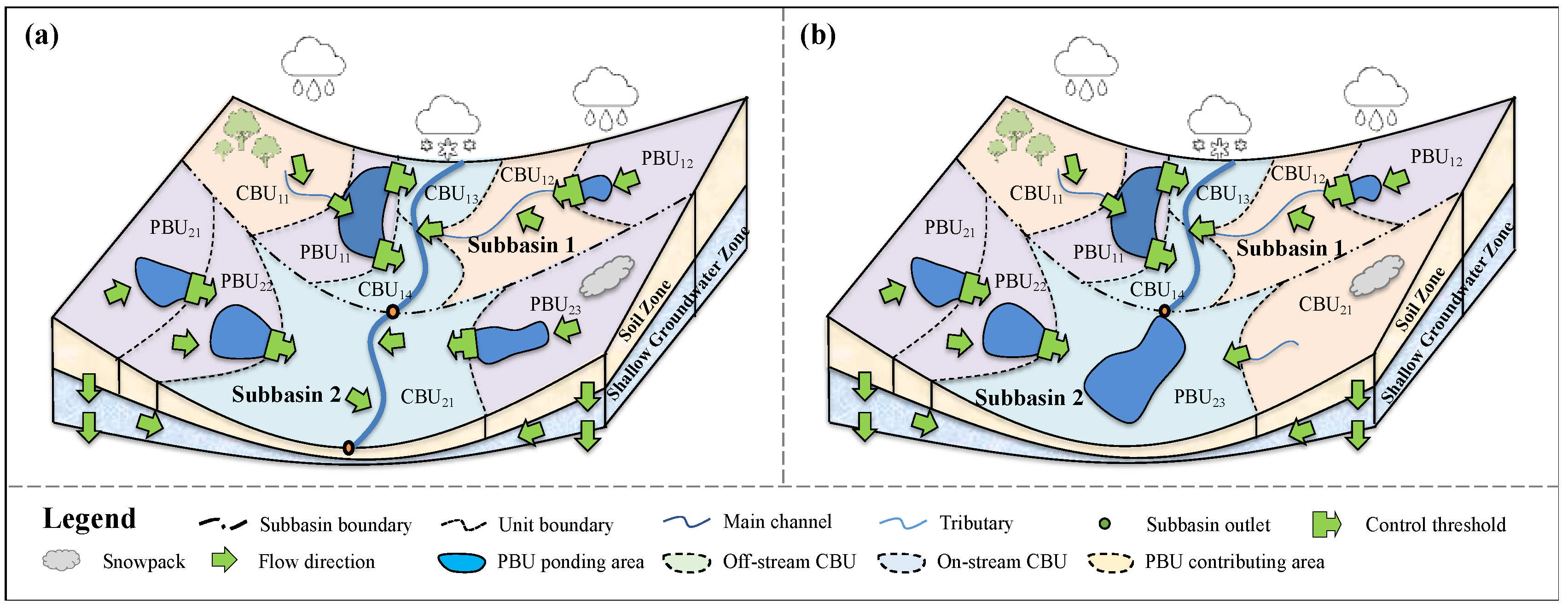
HYDROL-DC is a daily and semi-distributed hydrologic model that utilizes a physically based approach to simulate hydrologic processes related to lakes and rivers at watershed scales [48]. As illustrated in Figure 3a, HYDROL-DC divides a watershed into several sub-basins, and each sub-basin can be further divided into one main channel and several puddle-based units (PBUs) and channel-based units (CBUs). CBUs are further classified into on-stream CBUs, which interact directly with the main channel, and off-stream CBUs, which have no direct interaction. Each PBU is composed of a ponding area and its associated contribution area, and each CBU is composed of a channel segment (a main channel or tributary channel) and its associated contribution area. Surface runoff in a PBU transfers from the contribution area to the ponding area and is eventually released to its downstream unit when the storage capacity of the ponding area is exceeded. Surface runoff in a CBU runs directly into its tributary channel or the main channel.
Vertically, each unit is divided into five zones including the canopy zone, snow zone, surface zone, upper soil zone, and lower soil zone. Additionally, all units in a sub-basin share the same shallow groundwater zone. The upper soil zone can be further divided into multiple cells to simulate the soil water content at different depths, whereas the lower soil zone is lumped together with a reservoir function controlling percolation to the shallow groundwater zone. The major processes in each zone are listed in Table 1. To account for the closed characteristic of the study area, HYDROL-DC was modified by allowing a lake to serve as the outlet of a sub-basin (Figure 3b). In this study, the HJN watershed was divided into 8 sub-basins and each sub-basin contains only one unit.

2.4. Data Collected

2.4.1. Input Data

Table 2 lists the major input data utilized in HYDROL-DC, which include topographic data (e.g., sub-basin area and average elevation, the maximum ponding area and storage of each lake, and the length and slope of each river), precipitation, air temperature, leaf area index, potential ET, SCS curve number, and soil properties (e.g., saturated hydraulic conductivity, wilting point, and field capacity). The topographic data were calculated using ArcGIS based on the ALOS Global Digital Surface Model. The daily precipitation data were obtained from the China Meteorological Forcing Dataset [49] to calculate the average daily precipitation of each sub-basin. The leaf area index and air temperature were downloaded from the Global Land Surface Satellite dataset [50]. The potential ET of each sub-basin was estimated using the Hargreaves method, which considered the minimum and maximum temperatures [51]. The curve numbers of all sub-basins were calculated based on the Global Curve Number data [52]. Soil properties of all sub-basins were calculated using the Saxton Equation [53] based on the percentages of clay and sand recorded in the Harmonized World Soil Database v1.2 [54]. Groundwater routing was handled using a linear reservoir function, and the parameters of the groundwater zone were determined based on Yang et al. (2019) [55].

2.4.2. Evaluation Data

The daily observed ET of each sub-basin was calculated using a Harmonized Global Land Evaporation dataset from model-based products covering 1980–2017 [56]. To determine lake areas, Landsat-8 data was downloaded from the Geospatial Data Cloud (http://www.gscloud.cn/search (accessed on 23 August 2022)) and the Normalized Difference Water Index (NDWI) method [57] was applied to calculate lake areas based on the band 3 and band 6 (i.e., green light and near-infrared bands) of the Landsat-8 data (Equation (1)). Table 3 lists all the lake areas used in this study and their imaging dates.
N D W I = ( G r e e n N I R ) / ( G r e e n + N I R )
where G r e e n and N I R are the reflectance of green light and near-infrared bands, respectively.
Yang (2014) [58] calculated the natural average annual surface runoff and the consumptions caused by land cover change, climate change, reservoir construction, and domestic usage in the HJN watershed. In this study, the actual average annual surface runoff of each sub-basin was calculated based on the above values (Table 4). In addition, Yang (2014) [58] estimated the average annual groundwater discharge, which was 649 × 104 m3/a.

2.5. Model Setup and Performance Evaluation

The construction of the Zhasake reservoir has a significant impact on the inflow from the Zhasake River to HJN Lake; therefore, we selected the data from 2005 to 2017 for hydrologic modeling. The years 2005–2007 (i.e., 1 January 2005–31 December 2007) were selected as the warming-up period to set the initial conditions of the model, and the model calibration and validation periods were 1 January 2008–31 December 2013, and 1 January 2014–31 December 2017, respectively. A dimensionless sensitivity index (I) [59,60] was utilized for sensitivity analysis. Since this study focused on lake variations, the simulation output in the sensitivity analysis was specified as the mean of lake areas, and the percentage adjustment of each calibrated input parameter was set to 10%.
I = ( S 2 S 1 ) / S 0 2 Δ P / P 0
where Δ P is the percentage adjustment of an input parameter; S 0 , S 1 and S 2 are the simulation outputs when the input parameter equals P 0 , P 0 Δ P and P 0 + Δ P , respectively.
After the sensitivity analysis, three statistical parameters, including the Nash–Sutcliffe efficiency (NSE) coefficient, percent bias (PBIAS), and Pearson correlation coefficient (r), were used to evaluate the performance of HYDROL-DC in simulating ET of all sub-basins and the area of HJN Lake based on the performance ratings summarized by Moriasi et al. (2007) [61]. The NSE, PBIAS, and r can, respectively, be expressed as:
N S E = 1 i = 1 N ( O i S i ) 2 i = 1 N ( O i O ¯ ) 2
P B I A S = i = 1 N ( O i S i ) i = 1 N O i × 100
r = i = 1 N ( O i O ¯ ) ( S i S ¯ ) i = 1 N ( O i O ¯ ) 2 i = 1 N ( S i S ¯ ) 2
where O i is the value of the ith observed data, S i is the value of the ith simulated data, O ¯ is the mean value of the observed data, and N is the dataset size.

2.6. Analyses of Lake Variation and Impact Factors

The hydrologic processes that directly control the variations of HJN Lake include: (1) rainfall and snowmelt over the lake surface; (2) inflow from the contribution area of HJN Lake (i.e., CA inflow); (3) inflow from upstream rivers (i.e., upstream inflow); (4) the groundwater discharge to the lake (i.e., groundwater inflow); and (5) evaporation from the lake surface. In this study, the daily and annual variation characteristics of these processes were analyzed to reveal the mechanisms behind the dynamic changes in HJN Lake. The ratio of the annual inflow from each river to the annual upstream inflow of HJN Lake was calculated to quantify the contribution of each river to the lake variations. For each river, the relative standard deviation of the ratios in different years was calculated to analyze the stability of the inflow from each river to HJN Lake (Equation (6)). In addition, to access the impact of each hydrologic process on lake variations, the entire simulation period was divided into an increase stage (when the lake storage increased) and a decrease stage (when the lake storage decreased), and the linear regression method and Pearson correlation coefficient (Equation (5)) were used to analyze the correlations between each hydrologic process and the variations of lake storage at daily and monthly time scales.
R S D = 1 N 1 i = 1 N ( x i x ¯ ) 2 / x ¯
where R S D is the relative standard deviation, x i is the value of the ith sample point, x ¯ is the mean value of a sample, N is the sample size.

3. Results

3.1. Evaluation of Model Performance

Table 5 lists the calibrated parameters and their sensitivity index values (i.e., I). The curve number and lake evaporation coefficient were extremely sensitive to the area of HJN Lake, followed by the shallow groundwater percolation coefficient, initial abstraction, and an empirical evapotranspiration parameter (i.e., C2et). According to the sensitivity analysis, surface runoff and lake evaporation had significant influences on the variations of HJN Lake, and the shallow groundwater percolation coefficient impacted the groundwater inflow of the lake. Thus, these parameters were mainly adjusted in the calibration process. In addition, the other less sensitive parameters in Table 5 were also calibrated to improve the simulation results.
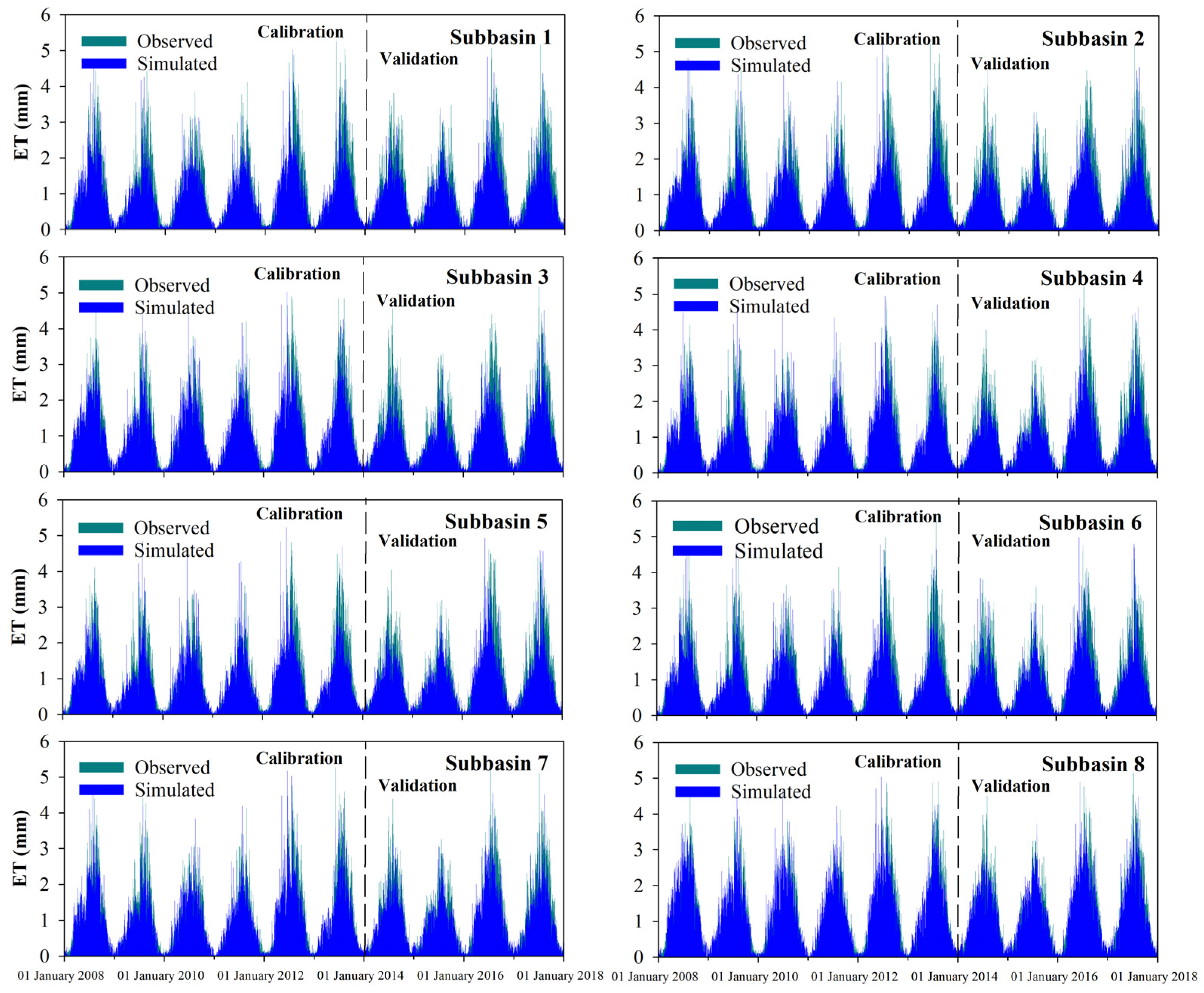
Figure 4 compares the simulated and observed ET for all sub-basins. Throughout the simulation period, the simulated ET shows a similar trend to the observed data. The coefficient of correlation (r) ranged from 0.82 to 0.87 in the calibration period and from 0.79 to 0.83 in the validation period, indicating a high degree of agreement between the simulated and observed trends in the variations of daily ET. Due to the underestimation of potential ET by using the Hargraves equation, the simulated ET from July to October was lower than the observed values. The ET of sub-basin eight was overestimated from April to June, which can be attributed to the constant lake evaporation coefficient used in HYDROL-DC. In general, HYDROL-DC slightly overestimated the ET of sub-basin eight and underestimated the ET of other sub-basins. The PBIAS values ranged from −8.52% to +18.21% in the calibration period and from −2.08% to 23.61% in the validation period, indicating the deviation between the simulated and observed ET. The ranges of NSE values were 0.63–0.74 and 0.56–0.67 for the calibration and validation periods, respectively. According to Moriasi et al. (2007) [61], the simulation results were rated between satisfactory and good.
The average annual surface runoff of each sub-basin was calculated and compared with the reference value from Yang (2014) [59] (Table 6). The simulation error ranged from −9.54% to +9.64%, with the largest error in sub-basin eight and the smallest in sub-basin six. In general, HYDROL-DC slightly overestimated the surface runoff in most sub-basins, except for sub-basins four and eight. For groundwater evaluation, the simulated average annual groundwater discharge was 605.13 × 10⁴ m3, with a simulation error of −6.67% compared to the reference value (i.e., 649 × 104 m3). Overall, HYDROL-DC successfully simulated the annual surface runoff for all sub-basins and the groundwater discharge to HJN Lake.
Figure 5 shows the simulated and observed areas of HJN Lake in the calibration and validation periods. The values of r, NSE, and PBIAS in the calibration period were 0.93, 0.71, and +1.89%, respectively, and those values in the validation period were 0.96, 0.65, and +1.11%, respectively. As shown in Figure 5, the variations of the simulated lake areas followed a similar trend to the observed areas with some underestimation in dry years (e.g., 2012 and 2015) due to the relatively simple groundwater module of the HYDROL-DC model. The high r values indicated a close similarity between the simulated and observed trends in the variations of the lake area. Furthermore, according to Moriasi et al. (2007) [61], the values of NSE and PBIAS were rated between good and very good for both the calibration and validation periods.
In summary, the r values were all greater than 0.79, indicating that the simulated ET and lake area had significant linear correlations with their observed values, respectively. The values of NSE mostly ranged from 0.65 to 0.74, most of the PBIAS values were within ±20%, and all the errors were smaller than ±10% during the entire simulation period. Therefore, according to Moriasi et al. (2007) [61], the overall performance of the HYDROL-DC in simulating hydrologic processes and lake areas can be rated as good. Considering the data shortage in the HJN watershed, the proposed approach yielded reasonable simulation results.

3.2. Hydrologic Process Analysis

The daily rainfall and snowmelt, evaporation, and lake storage are shown in Figure 6a, and Figure 6b depicts the daily CA inflow, upstream inflow, groundwater inflow, and lake area. Both figures were combined to analyze the dynamic characteristics of all hydrologic processes and the influence of these processes on lake variations. According to Figure 6, rainfall was concentrated from July to September, and the CA inflow, upstream inflow, and groundwater inflow were mainly generated after rainfall events. Additionally, inflows also could be generated in early spring (e.g., March 2016) and the end of fall (e.g., November 2015) due to snowmelt. In terms of the recession rate, the groundwater inflow had the lowest rate, followed by upstream inflow and CA inflow (Figure 6b). The storage and area of HJN Lake continued to increase after rainfall and snowmelt, and this increase continued into winter if there was sufficient supplementation (e.g., in the winter of 2013). The reduction in the storage and area typically occurred in spring and early summer due to increased evaporation (Figure 6a) and inadequate water supply (Figure 6b).
Figure 7 and Table 7 show the annual water balance of HJN Lake. The source terms of HJN Lake included rainfall and snowmelt, CA inflow, upstream inflow, and groundwater inflow. Evaporation was the sink term of HJN Lake, with an average value of 125 mm. Based on the storage variations of HJN Lake, the entire simulation period can be divided into a decrease period (2008–2011), a fluctuation period (2012–2015), and an increase period (2016–2017). During the decrease period, the evaporation was greater than its average value, and lake storage decreased by 346.84 mm due to the significant evaporation and insufficient water supply. Rainfall and snowmelt were the main factors maintaining the lake storage during this period. As the drought continued, the proportion of rainfall and snowmelt in the total water supply of HJN Lake gradually increased from 52.54% to 95.25%. In the fluctuation period, due to the changes in the total water supply and evaporation, lake storage increased by 69.88 mm from 2012 to 2013 and then decreased by 124.32 mm from 2014 to 2015. The proportion of each source term in the total supply changed alternately, with the variation in groundwater inflow lagging behind other source terms. In the increase period, lake storage increased by 256.49 mm. Compared with rainfall and snowmelt, surface and groundwater inflows contributed the most water to HJN Lake. In 2016 and 2017, the proportion of the inflows in the total water supply was 82.80% and 78.83%, respectively. The relative standard deviations of the annual rainfall and snowmelt, CA inflow, upstream inflow, and groundwater inflow were 0.33, 1.41, 1.12, and 1.10, respectively. Therefore, rainfall and snowmelt provided the most stable supplement to HJN Lake, followed by groundwater inflow, upstream inflow, and CA inflow.
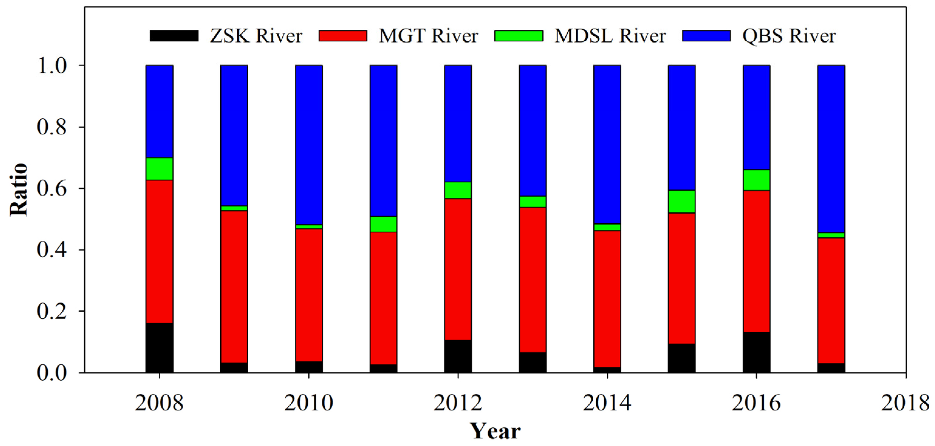
Figure 8 shows the ratio of the annual inflow from each river to the annual upstream inflow of HJN Lake. Based on the surface delineation results shown in Figure 1, the contribution areas of Mudushili River and Qibosu River are sub-basins three and six, respectively. The contributing area of the Zhasake River is composed of sub-basins one, two, and seven, and the contribution area of the Manggaitu River is composed of sub-basins four and five. The ratio of the inflow from the Manggaitu River to the upstream inflow ranged from 0.41 to 0.50, while for the Qibosu River, Zhasake River, and Mudushili River, the ranges were 0.30–0.54, 0.02–0.16, and 0.01–0.07, respectively. The average ratio of the inflow from the Manggaitu River to the upstream inflow was 0.45, followed by the Qibosu River (0.44), Zhasake River (0.07), and Mudushili River (0.04). Thus, the Manggaitu River and Qibosu River contributed the most surface runoff to HJN Lake throughout the simulation period. Furthermore, the supply stability of each river was quantified by calculating the relative standard deviation of the ratios in different years. Accordingly, the Manggaitu River was the most stable (RSD = 0.06), followed by the Qibosu River (RSD = 0.19), Mudushili River (RSD = 0.58), and Zhasake River (RSD = 0.73).

3.3. Correlation Analysis

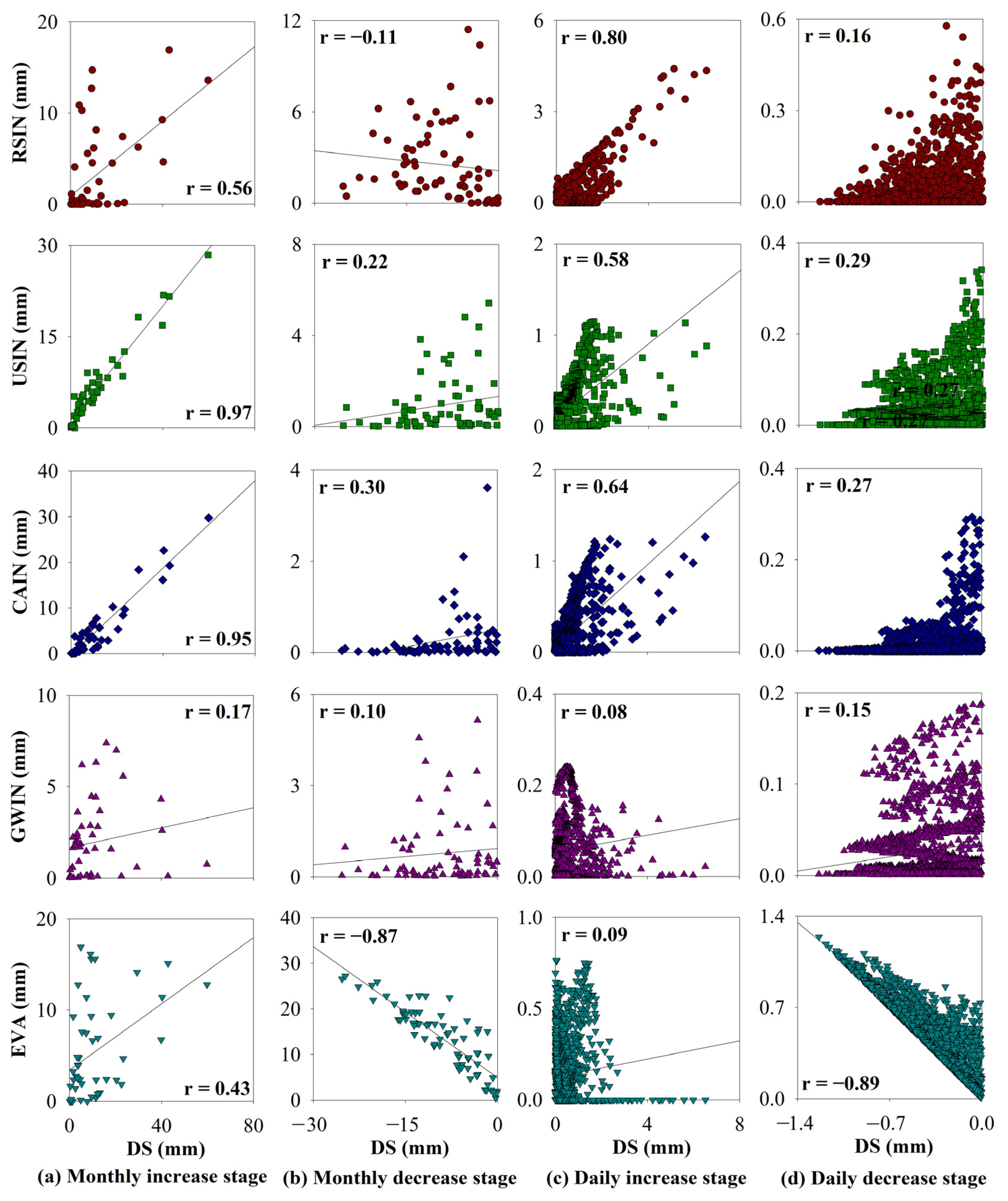
The correlations between the storage variation of HJN Lake and the water balance terms at monthly and daily time scales are shown in Figure 9. The storage variation was categorized into two conditions: an increase condition (variation greater than zero) and a decrease condition (variation less than zero). At the monthly time scale, the two major factors that increased the lake storage were upstream inflow (r = 0.97) and CA inflow (r = 0.95) (Figure 9a). In contrast, rainfall and snowmelt had a weaker correlation with the storage variation (r = 0.56). Evaporation was found to be the factor causing the decrease in lake storage (Figure 9b) and had a strong negative linear relationship with the variation in lake storage (r = −0.87). At the daily time scale, rainfall and snowmelt were the most significant factors that increased the lake storage (r = 0.80), followed by the CA inflow (r = 0.64) and upstream inflow (r = 0.58) (Figure 9c). Similar to the results at the monthly time scale, evaporation had a strong negative linear relationship with the variation in the lake storage at the daily time scale, with a coefficient of correlation of −0.89 (Figure 9d). The groundwater inflow had little correlation with the storage variation, which might be due to the small quantity and the low recession rate of the groundwater inflow.

4. Discussion

4.1. Criteria and Results of Model Evaluation

This study aimed to solve the contradiction between data shortage and the requirement for detailed hydrological information in semi-arid and ungauged closed watersheds. Previous studies have confirmed the effectiveness of utilizing remote-sensed ET data for model evaluation in such areas [42,43,44]. Based on the hydrological characteristics of lakes in semi-arid regions [13,30,58], in addition to the remote-sensed ET data, we also used remotely sensed lake areas and the results from previous studies for model evaluation. The calibration and validation results indicated that the simulated ET was between satisfactory and good in general and underestimation mainly occurred from July to October. This phenomenon has been observed in previous studies and can be attributed to the underestimation of potential ET in semi-aired regions by using the Hargraves equation [62,63,64]. Throughout the simulation period, the simulated lake area corresponded well with the observed values. However, due to the simplification of groundwater, the simulated lake area decreased faster than the observed values in some dry years (e.g., 2011 and 2015). HYDROL-DC employs a linear reservoir function to simulate groundwater discharge based on soil percolation, resulting in possible underestimation of discharge when there is no sufficient replenishment. Previous studies using similar functions had the same issue in simulating groundwater discharge under dry climate conditions [65,66,67].

4.2. Comparison with Previous Studies

Most previous studies in semi-arid and ungauged closed watersheds used remote-sensing data and water-balance models to analyze monthly and annual lake variations [25,26,27,28,29,30]. This study provides a valuable supplement to these previous studies and can address the gaps in simulating detailed hydrologic processes related to lakes. In the HJN watershed, previous studies identified precipitation and evaporation (or temperature) as the meteorological driving factors influencing lake variations [68,69,70], and surface runoff and evaporation were identified as the hydrologic driving factors [30]. These results were consistent with the annual mass balance in our study. In addition, our study utilized the daily simulation results to reveal the linkage between hydrologic processes and lake variations: (1) rainfall and snowmelt were the most stable supplements to HJN Lake due to their instantaneous supply mechanism; (2) compared with rainfall and snowmelt, the generation of groundwater inflow, upstream inflow, and CA inflow were relatively more susceptible to climate and soil conditions, and therefore had greater effects on the water supplement of HJN Lake in wet years rather than dry years (Figure 7 and Table 7); (3) the stability of groundwater inflow was followed by upstream inflow and CA inflow due to the differences in their recession rates (Figure 6).
Liang and Li (2019) [69] reported that precipitation and ET had a positive and negative correlation, respectively, with the area of HJN Lake. The coefficient of correlation varied at monthly, seasonal, and annual time scales. Our study yielded similar results, which can be attributed to the generation mechanisms of hydrologic processes. The correlation analysis showed that evaporation dominated the decrease of lake storage (Figure 9b,d), and the coefficient of correlation was slightly greater at the daily time scale than at the monthly time scale due to the instantaneous generation mechanism of lake evaporation. At the daily time scale, rainfall and snowmelt showed a stronger correlation with the increase of lake storage compared to the CA inflow and upstream inflow, while the correlation was weaker at the monthly time scale. The upstream inflow showed a stronger correlation with the increase of lake storage compared to the CA inflow, whereas the correlation was weaker at the daily time scale. These findings can be explained by the following reasons: (1) rainfall and snowmelt over the lake have an immediate impact on increasing lake storage; (2) the CA inflow originates in the contribution area of HJN Lake and supplies the lake after surface runoff routing; and (3) in comparison to the CA inflow, the upstream inflow requires channel routing before supplying HJN Lake, in addition to the runoff generation and surface runoff routing processes. Additionally, Liang and Li (2019) [69] found the correlations between meteorological driving factors, especially precipitation, and lake area had a lag period of approximately 1–3 months at the monthly time scale. This can be observed in Figure 6 and explained by the generation mechanisms of hydrologic processes related to HJN Lake.

4.3. Guidance for Local Water Management

The new approach can enhance our comprehension of the water cycle in semi-aired and ungauged closed watersheds, and guide local water resource management. Though HJN Lake expanded in 2016 and 2017, previous studies (e.g., [30,70]) and our research show that the expansion was due to increased precipitation. Therefore, it is still essential to implement scientific management policies to protect HJN Lake and its associated ecological system. Precipitation and surface runoff are the main sources of water supply for HJN Lake, and the Manggaitu River and Qibosu River are the most significant and stable rivers that contribute water to HJN Lake. Therefore, conserving surface runoff, particularly the streamflow of the Manggaitu River and Qibosu River, may be an efficient way to prevent the shrinkage of HJN Lake.

4.4. Limitations and Future Work

The results of this study are subject to the influences of input data and model functions. Since most of the input data were processed from remote-sensing data with resolutions of 250 m and 1 km, using high-resolution data can enhance the accuracy of this study. It has been observed in many studies that the Hargreaves equation tends to underestimate the potential ET in semi-arid regions, indicating that the equation should be adapted for specific locations [62,63,64]. However, due to the lack of observed data, this study utilized the original equation to calculate the potential ET of the HJN watershed. Therefore, obtaining more observed meteorological data can improve the calculated potential ET. Moreover, the groundwater module of the HYDROL-DC model is relatively basic, which may cause the underestimation of groundwater flow during long-term drought conditions. To address this issue, future studies can consider enhancing the HYDROL-DC model by integrating it with groundwater models such as MODFLOW.

5. Conclusions

In this study, a comprehensive approach was proposed to simulate lake variations in semi-arid and ungauged closed watersheds and analyze potential hydrologic driving factors of the variations. Unlike previous studies that used water-balance models, the new approach integrated lake-oriented and physically based hydrologic modeling, remote-sensing data, and results from previous studies to reveal detailed hydrologic processes related to lake variations.
The application in the HJN watershed demonstrated that using remote-sensed ET and lake area data and the results from previous studies effectively solved the data shortage issue in applying physically based hydrologic models to the HJN watershed. During the entire simulation period, rainfall and snowmelt were the most stable supplements to HJN Lake, followed by groundwater inflow, upstream inflow, and CA inflow, due to the differences in their generation mechanisms. In the decrease period (i.e., 2008–2011), rainfall and snowmelt were the major supplements of HJN Lake, while the CA inflow, upstream inflow, and groundwater inflow dominated lake variations in the increase period (2016–2017). Different rivers displayed distinct contributions to HJN Lake, with the Manggaitu River and Qibosu River being the primary and most stable rivers. The generation mechanisms also influenced the correlations between each hydrologic process and the storage variation of HJN Lake at different time scales. The correlation analysis revealed that evaporation dominated the shrinkage of HJN Lake, with the coefficient of correlation at the daily time scale slightly greater than that at the monthly time scale. Rainfall and snowmelt were the key factors for lake storage increase at the daily time scale, while the upstream inflow and CA inflow were the major factors at the monthly time scale.
Overall, the approach proposed in this study effectively simulated the detailed variations and associated hydrologic processes of HJN Lake. The results of this study can not only enhance our comprehension of the hydrological processes related to HJN Lake but also provide valuable guidance for local water resources management and ecological protection. Moreover, this approach can serve as an alternative option for hydrological simulation in other semi-arid and ungauged closed watersheds.

Author Contributions

Conceptualization, N.W. and Y.X.; methodology, N.W., J.Y., Z.Z. and Y.X.; software, N.W. and J.Y.; validation, N.W., Z.Z. and Y.X.; formal analysis, N.W., J.Y. and L.Y.; investigation, N.W., J.Y., Z.Z. and H.W.; resources, J.Y., H.W. and J.H.; data curation, N.W., H.W. and J.H.; writing—original draft preparation, N.W.; writing—review and editing, Z.Z., Y.X., H.W. and J.H.; visualization, J.Y. and L.Y.; supervision, N.W.; project administration, N.W.; funding acquisition, N.W. All authors have read and agreed to the published version of the manuscript.

Funding

This research was funded by the National Natural Science Foundation of China (Grant No. 42107067), the Natural Science Foundation of Sichuan Province (2022NSFSC1084), the Fundamental Research Funds for the Central Universities (Grant No. 300102292101), and the China Postdoctoral Science Foundation (Grant No. 2021M692745).

Institutional Review Board Statement

Not applicable.

Informed Consent Statement

Not applicable.

Data Availability Statement

The data presented in this study are available on request from the corresponding author.

Conflicts of Interest

The authors declare no conflict of interest.

References

  1. Fu, C.; Wu, H.; Zhu, Z.; Song, C.; Xue, B.; Wu, H.; Ji, Z.; Dong, L. Exploring the potential factors on the striking water level variation of the two largest semi-arid-region lakes in northeastern Asia. Catena 2022, 1198, 105037. [Google Scholar] [CrossRef]
  2. Wurtsbaugh, W.A.; Miller, C.; Null, S.E.; DeRose, J.; Wilcock, P.; Hahnenberger, M.; Howe, F.; Moore, J. Decline of the world’s saline lakes. Nat. Geosci. 2017, 10, 816–823. [Google Scholar] [CrossRef]
  3. Chen, J.; Qian, H.; Gao, Y.; Wang, H.; Zhang, M. Insights into hydrological and hydrochemical processes in response to water replenishment for lakes in arid regions. J. Hydrol. 2020, 581, 124386. [Google Scholar] [CrossRef]
  4. Janssen, A.B.; Van Wijk, D.; Van Gerven, L.P.; Bakker, E.S.; Brederveld, R.J.; DeAngelis, D.L.; Janse, J.H.; Mooij, W.M. Success of lake restoration depends on spatial aspects of nutrient loading and hydrology. Sci. Total Environ. 2019, 679, 248–259. [Google Scholar] [CrossRef] [PubMed]
  5. Tan, C.; Guo, B.; Kuang, H.; Yang, H.; Ma, M. Lake area changes and their influence on factors in arid and semi-arid regions along the silk road. Remote Sens. 2018, 10, 595. [Google Scholar] [CrossRef] [Green Version]
  6. Murumkar, A.; Durand, M.; Fernández, A.; Moritz, M.; Mark, B.; Phang, S.C.; Laborde, S.; Scholte, P.; Shastry, A.; Hamilton, I. Trends and spatial patterns of 20th century temperature, rainfall and PET in the semi-arid Logone River basin, Sub-Saharan Africa. J. Arid Environ. 2020, 178, 104168. [Google Scholar] [CrossRef]
  7. Yan, X.; Liu, J.; Rühland, K.M.; Smol, J.P.; Chen, F. Climate change as the dominant driver of recent ecological changes in a semi-arid alpine lake from the Chinese Loess Plateau. J. Paleolimnol. 2022, 68, 39–57. [Google Scholar] [CrossRef]
  8. Jeppesen, E.; Beklioğlu, M.; Özkan, K.; Akyürek, Z. Salinization increase due to climate change will have substantial negative effects on inland waters: A call for multifaceted research at the local and global scale. Innovation 2020, 1, 100030. [Google Scholar] [CrossRef]
  9. Cooley, S.W.; Ryan, J.C.; Smith, L.C. Human alteration of global surface water storage variability. Nature 2021, 591, 78–81. [Google Scholar] [CrossRef]
  10. Zhang, Y.; Liang, W.; Liao, Z.; Han, Z.; Xu, X.; Jiao, R.; Liu, H. Effects of climate change on lake area and vegetation cover over the past 55 years in Northeast Inner Mongolia grassland, China. Theor. Appl. Climatol. 2019, 138, 13–25. [Google Scholar] [CrossRef]
  11. Wang, J.; Ding, J.; Li, G.; Liang, J.; Yu, D.; Aishan, T.; Zhang, F.; Yang, J.; Abulimiti, A.; Liu, J. Dynamic detection of water surface area of Ebinur Lake using multi-source satellite data (Landsat and Sentinel-1A) and its responses to changing environment. Catena 2019, 177, 189–201. [Google Scholar] [CrossRef]
  12. Wufu, A.; Wang, H.; Chen, Y.; Rusuli, Y.; Ma, L.; Yang, S.; Zhang, F.; Wang, D.; Li, Q.; Li, Y. Lake water volume fluctuations in response to climate change in Xinjiang, China from 2002 to 2018. PeerJ 2020, 8, 9683. [Google Scholar] [CrossRef] [PubMed]
  13. Gxokwe, S.; Dube, T.; Mazvimavi, D. Multispectral remote sensing of wetlands in semi-arid and arid areas: A review on applications, challenges and possible future research directions. Remote Sens. 2020, 12, 4190. [Google Scholar] [CrossRef]
  14. Zhang, Y.; Zhang, Y.; Shi, K.; Zhou, Y.; Li, N. Remote sensing estimation of water clarity for various lakes in China. Water Res. 2021, 192, 116844. [Google Scholar] [CrossRef]
  15. Huovinen, P.; Ramírez, J.; Caputo, L.; Gómez, I. Mapping of spatial and temporal variation of water characteristics through satellite remote sensing in Lake Panguipulli, Chile. Sci. Total Environ. 2019, 679, 196–208. [Google Scholar] [CrossRef]
  16. Wan, W.; Xiao, P.; Feng, X.; Li, H.; Ma, R.; Duan, H.; Zhao, L. Monitoring lake changes of Qinghai-Tibetan Plateau over the past 30 years using satellite remote sensing data. Chin. Sci. Bull. 2014, 59, 1021–1035. [Google Scholar] [CrossRef]
  17. Tulbure, M.G.; Broich, M.; Stehman, S.V.; Kommareddy, A. Surface water extent dynamics from three decades of seasonally continuous Landsat time series at subcontinental scale in a semi-arid region. Remote Sens. Environ. 2016, 178, 142–157. [Google Scholar] [CrossRef]
  18. Dang, A.T.; Kumar, L.; Reid, M.; Nguyen, H. Remote sensing approach for monitoring coastal wetland in the Mekong Delta, Vietnam: Change trends and their driving forces. Remote Sens. 2021, 13, 3359. [Google Scholar] [CrossRef]
  19. Hooker, J.; Duveiller, G.; Cescatti, A. Data descriptor: A global dataset of air temperature derived from satellite remote sensing and weather stations. Sci. Data 2018, 5, 180246. [Google Scholar] [CrossRef] [Green Version]
  20. Courty, L.G.; Soriano-Monzalvo, J.C.; Pedrozo-Acuña, A. Evaluation of open-access global digital elevation models (AW3D30, SRTM, and ASTER) for flood modelling purposes. J. Flood Risk Manag. 2019, 12, 12550. [Google Scholar] [CrossRef] [Green Version]
  21. Huang, Q.; Long, D.; Du, M.; Zeng, C.; Li, X.; Hou, A.; Hong, Y. An improved approach to monitoring Brahmaputra River water levels using retracked altimetry data. Remote Sens. Environ. 2018, 211, 112–128. [Google Scholar] [CrossRef]
  22. Shrestha, N.K.; Qamer, F.M.; Pedreros, D.; Murthy, M.S.R.; Wahid, S.M.; Shrestha, M. Evaluating the accuracy of Climate Hazard Group (CHG) satellite rainfall estimates for precipitation based drought monitoring in Koshi basin, Nepal. J. Hydrol. 2017, 13, 138–151. [Google Scholar] [CrossRef]
  23. Wilson, A.M.; Jetz, W. Remotely sensed high-resolution global cloud dynamics for predicting ecosystem and biodiversity distributions. PLoS Biol. 2016, 14, 1002415. [Google Scholar] [CrossRef] [PubMed]
  24. Wang, T.; Shi, J.; Husi, L.; Zhao, T.; Ji, D.; Xiong, C.; Gao, B. Effect of solar-cloud-satellite geometry on land surface shortwave radiation derived from remotely sensed data. Remote Sens. 2017, 9, 690. [Google Scholar] [CrossRef] [Green Version]
  25. Pandi, D.; Kothandaraman, S.; Kuppusamy, M. Hydrological models: A review. Int. J. Hydrol. Sci. Technol. 2021, 12, 223–242. [Google Scholar] [CrossRef]
  26. Tahmasebi Nasab, M.; Singh, V.; Chu, X. SWAT modeling for depression-dominated areas: How do depressions manipulate hydrologic modeling? Water 2017, 9, 58. [Google Scholar] [CrossRef] [Green Version]
  27. Zeng, L.; Chu, X. A new probability-embodied model for simulating variable contributing areas and hydrologic processes dominated by surface depressions. J. Hydrol. 2021, 602, 126762. [Google Scholar] [CrossRef]
  28. Liang, K. Quantifying streamflow variations in ungauged lake basins by integrating remote sensing and water balance modeling: A case study of the erdos larus relictus national nature reserve, China. Remote Sens. 2017, 9, 588. [Google Scholar] [CrossRef] [Green Version]
  29. Yang, X.; Lu, X.; Park, E.; Tarolli, P. Impacts of climate change on lake fluctuations in the Hindu Kush-Himalaya-Tibetan Plateau. Remote Sens. 2019, 11, 1082. [Google Scholar] [CrossRef] [Green Version]
  30. Yue, H.; Liu, Y. Water balance and influence mechanism analysis: A case study of Hongjiannao Lake, China. Environ. Monit. Assess. 2021, 193, 219. [Google Scholar] [CrossRef]
  31. Ala-Aho, P.; Rossi, P.M.; Isokangas, E.; Kløve, B. Fully integrated surface–subsurface flow modelling of groundwater–lake interaction in an esker aquifer: Model verification with stable isotopes and airborne thermal imaging. J. Hydrol. 2015, 522, 391–406. [Google Scholar] [CrossRef]
  32. Adnan, M.; Kang, S.; Zhang, G.; Saifullah, M.; Anjum, M.N.; Ali, A.F. Simulation and analysis of the water balance of the Nam Co Lake using SWAT model. Water 2019, 11, 1383. [Google Scholar] [CrossRef] [Green Version]
  33. Zeng, L.; Shao, J.; Chu, X. Improved hydrologic modeling for depression-dominated areas. J. Hydrol. 2020, 590, 125269. [Google Scholar] [CrossRef]
  34. Bhattacharjee, J.; Rabbil, M.; Fazel, N.; Darabi, H.; Choubin, B.; Khan, M.M.R.; Marttila, H.; Haghighi, A.T. Accuracy assessment of remotely sensed data to analyze lake water balance in semi-arid region. Sci. Total Environ. 2021, 797, 149034. [Google Scholar] [CrossRef] [PubMed]
  35. Moknatian, M.; Piasecki, M. Development of predictive models for water budget simulations of closed-basin lakes: Case studies of Lakes Azuei and Enriquillo on the Island of Hispaniola. Hydrology 2021, 8, 148. [Google Scholar] [CrossRef]
  36. Lu, J.; Chen, X.; Zhang, L.; Sauvage, S.; Sánchez-Pérez, J.M. Water balance assessment of an ungauged area in Poyang Lake watershed using a spatially distributed runoff coefficient model. J. Hydroinform. 2018, 20, 1009–1024. [Google Scholar] [CrossRef]
  37. Li, Z.; Lei, X.; Liao, W.; Yang, Q.; Cai, S.; Wang, X.; Wang, C.; Wang, J. Lake inflow simulation using the coupled water balance method and Xin’anjiang Model in an ungauged stream of Chaohu Lake Basin, China. Front. Earth Sci. 2021, 9, 615692. [Google Scholar] [CrossRef]
  38. Garavaglia, F.; Le Lay, M.; Gottardi, F.; Garçon, R.; Gailhard, J.; Paquet, E.; Mathevet, T. Impact of model structure on flow simulation and hydrological realism: From a lumped to a semi-distributed approach. Hydrol. Earth Syst. Sci. 2017, 21, 3937–3952. [Google Scholar] [CrossRef] [Green Version]
  39. Das, T.; Bárdossy, A.; Zehe, E.; He, Y. Comparison of conceptual model performance using different representations of spatial variability. J. Hydrol. 2008, 356, 106–118. [Google Scholar] [CrossRef]
  40. López López, P.; Sutanudjaja, E.H.; Schellekens, J.; Sterk, G.; Bierkens, M.F. Calibration of a large-scale hydrological model using satellite-based soil moisture and evapotranspiration products. Hydrol. Earth Syst. Sci. 2017, 21, 3125–3144. [Google Scholar] [CrossRef] [Green Version]
  41. Sirisena, T.J.G.; Maskey, S.; Ranasinghe, R. Hydrological model calibration with streamflow and remote sensing based evapotranspiration data in a data poor basin. Remote Sens. 2020, 12, 3768. [Google Scholar] [CrossRef]
  42. Pan, S.; Xu, Y.P.; Gu, H.; Yu, B.; Xuan, W. Evaluation of Remote Sensing-Based Evapotranspiration Datasets for Improving Hydrological Model Simulation in Humid Region of East China. Remote Sens. 2022, 14, 4546. [Google Scholar] [CrossRef]
  43. Ha, L.T.; Bastiaanssen, W.G.; Van Griensven, A.; Van Dijk, A.I.; Senay, G.B. Calibration of spatially distributed hydrological processes and model parameters in SWAT using remote sensing data and an auto-calibration procedure: A case study in a Vietnamese river basin. Water 2018, 10, 212. [Google Scholar] [CrossRef] [Green Version]
  44. Bennour, A.; Jia, L.; Menenti, M.; Zheng, C.; Zeng, Y.; Asenso Barnieh, B.; Jiang, M. Calibration and validation of SWAT model by using hydrological remote sensing observables in the Lake Chad Basin. Remote Sens. 2022, 14, 1511. [Google Scholar] [CrossRef]
  45. Yue, H.; Li, Y.; Qian, J.; Liu, Y. A new accuracy evaluation method for water body extraction. Int. J. Remote Sens. 2020, 41, 7311–7342. [Google Scholar] [CrossRef]
  46. Cao, H.; Han, L.; Liu, Z.; Li, L. Monitoring and driving force analysis of spatial and temporal change of water area of Hongjiannao Lake from 1973 to 2019. Ecol. Inform. 2021, 61, 101230. [Google Scholar] [CrossRef]
  47. Wang, N.; Chu, X. A new algorithm for delineation of surface depressions and channels. Water 2019, 12, 7. [Google Scholar] [CrossRef] [Green Version]
  48. Wang, N.; Chu, X.; Zhang, X. Functionalities of surface depressions in runoff routing and hydrologic connectivity modeling. J. Hydrol. 2021, 593, 125870. [Google Scholar] [CrossRef]
  49. He, J.; Yang, K.; Tang, W.; Lu, H.; Qin, J.; Chen, Y.Y.; Li, X. The first high-resolution meteorological forcing dataset for land process studies over China. Sci. Data 2020, 7, 25. [Google Scholar] [CrossRef] [PubMed] [Green Version]
  50. Liang, S.; Zhao, X.; Yuan, W.; Liu, S.; Cheng, X.; Xiao, Z.; Zhang, X.; Liu, Q.; Cheng, J.; Tang, H.; et al. A Long-term Global LAnd Surface Satellite (GLASS) Dataset for Environmental Studies. Int. J. Digit. Earth 2013, 6, 5–33. [Google Scholar] [CrossRef]
  51. Hargreaves, G.H.; Samani, Z.A. Estimating potential evapotranspiration. J. Irrig. Drain. Div. 1982, 108, 225–230. [Google Scholar] [CrossRef]
  52. Jaafar, H.H.; Ahmad, F.A.; El Beyrouthy, N. GCN250, new global gridded curve numbers for hydrologic modeling and design. Sci. Data 2019, 6, 145. [Google Scholar] [CrossRef] [Green Version]
  53. Saxton, K.E.; Rawls, W.; Romberger, J.S.; Papendick, R.I. Estimating generalized soil-water characteristics from texture. Soil Sci. Soc. Am. J. 1986, 50, 1031–1036. [Google Scholar] [CrossRef]
  54. Fischer, G.; Nachtergaele, F.; Prieler, S.; Van Velthuizen, H.T.; Verelst, L.; Wiberg, D. Global Agro-Ecological Zones Assessment for Agriculture (GAEZ 2008); Austria and FAO: Rome, Italy, 2008; p. 10. [Google Scholar]
  55. Yang, Z.Y.; Wang, K.; Yuan, Y.; Huang, J.; Chen, Z.J.; Li, C. Non-negligible lag of groundwater infiltration recharge: A case in Mu Us Sandy Land, China. Water 2019, 11, 561. [Google Scholar] [CrossRef] [Green Version]
  56. Lu, J.; Wang, G.; Chen, T.; Li, S.; Hagan, D.F.T.; Kattel, G.; Peng, J.; Jiang, T.; Su, B. A harmonized global land evaporation dataset from model-based products covering 1980–2017. Earth Syst. Sci. Data 2021, 13, 5879–5898. [Google Scholar] [CrossRef]
  57. McFeeters, S.K. The use of the Normalized Difference Water Index (NDWI) in the delineation of open water features. Int. J. Remote Sens. 1996, 17, 1425–1432. [Google Scholar] [CrossRef]
  58. Yang, L. Research on Comprehensive Regulation of Water Resources in Arid Inland River Basin from Ecological Perspective-with Hongjiannao Basin as the Study Objective. Ph.D. Dissertation, Xi’an University of Technology, Xi’an, China, 2014. (In Chinese). [Google Scholar]
  59. Lenhart, T.; Eckhardt, K.; Fohrer, N.; Frede, H.G. Comparison of two different approaches of sensitivity analysis. Phys. Chem. Earth 2002, 27, 645–654. [Google Scholar] [CrossRef]
  60. Ficklin, D.L.; Luo, Y.; Stewart, I.T.; Maurer, E.P. Development and application of a hydroclimatological stream temperature model within the Soil and Water Assessment Tool. Water Resour. Res. 2012, 48, W01511. [Google Scholar] [CrossRef] [Green Version]
  61. Moriasi, D.N.; Arnold, J.G.; Van Liew, M.W.; Bingner, R.L.; Harmel, R.D.; Veith, T.L. Model evaluation guidelines for systematic quantification of accuracy in watershed simulations. Trans. ASABE 2007, 50, 885–900. [Google Scholar] [CrossRef]
  62. Shahidian, S.; Serralheiro, R.; Serrano, J.; Teixeira, J.; Haie, N.; Santos, F. Hargreaves and Other Reduced-Set Methods for Calculating Evapotranspiration; IntechOpen: London, UK, 2012; pp. 59–80. [Google Scholar]
  63. Dan, Z.; Bo, Z. Effect of potential evapotranspiration estimation method on reconnaissance drought index (RDI) calculation. Chin. J. Agrometeorol. 2014, 35, 258. [Google Scholar]
  64. Xia, X.; Zhu, X.; Pan, Y.; Zhang, J. Hargreaves ET0 Equation Regression Correction and Parameter Spatialization for Mainland China. Appl. Eng. Agric. 2020, 36, 673–686. [Google Scholar] [CrossRef]
  65. Jin, X.; He, C.; Zhang, L.; Zhang, B. A modified groundwater module in SWAT for improved streamflow simulation in a large, arid endorheic river watershed in Northwest China. Chin. Geogr. Sci. 2018, 28, 47–60. [Google Scholar] [CrossRef] [Green Version]
  66. Shao, G.; Zhang, D.; Guan, Y.; Xie, Y.; Huang, F. Application of SWAT model with a modified groundwater module to the semi-arid Hailiutu River Catchment, Northwest China. Sustainability 2019, 11, 2031. [Google Scholar] [CrossRef] [Green Version]
  67. Geng, X.; Zhang, C.; Zhang, F.E.; Chen, Z.; Nie, Z.; Liu, M. Hydrological modeling of karst watershed containing subterranean river using a modified SWAT model: A case study of the Daotian River Basin, southwest China. Water 2021, 13, 3552. [Google Scholar] [CrossRef]
  68. Liang, K.; Yan, G. Application of landsat imagery to investigate lake area variations and relict gull habitat in hongjian lake, Ordos Plateau, China. Remote Sens. 2017, 9, 1019. [Google Scholar] [CrossRef] [Green Version]
  69. Liang, K.; Li, Y. Changes in lake area in response to climatic forcing in the endorheic Hongjian Lake Basin, China. Remote Sens. 2019, 11, 3046. [Google Scholar] [CrossRef] [Green Version]
  70. Yue, H.; Liu, Y. Variations in the lake area, water level, and water volume of Hongjiannao Lake during 1986–2018 based on Landsat and ASTER GDEM data. Environ. Monit. Assess. 2019, 191, 606. [Google Scholar] [CrossRef]
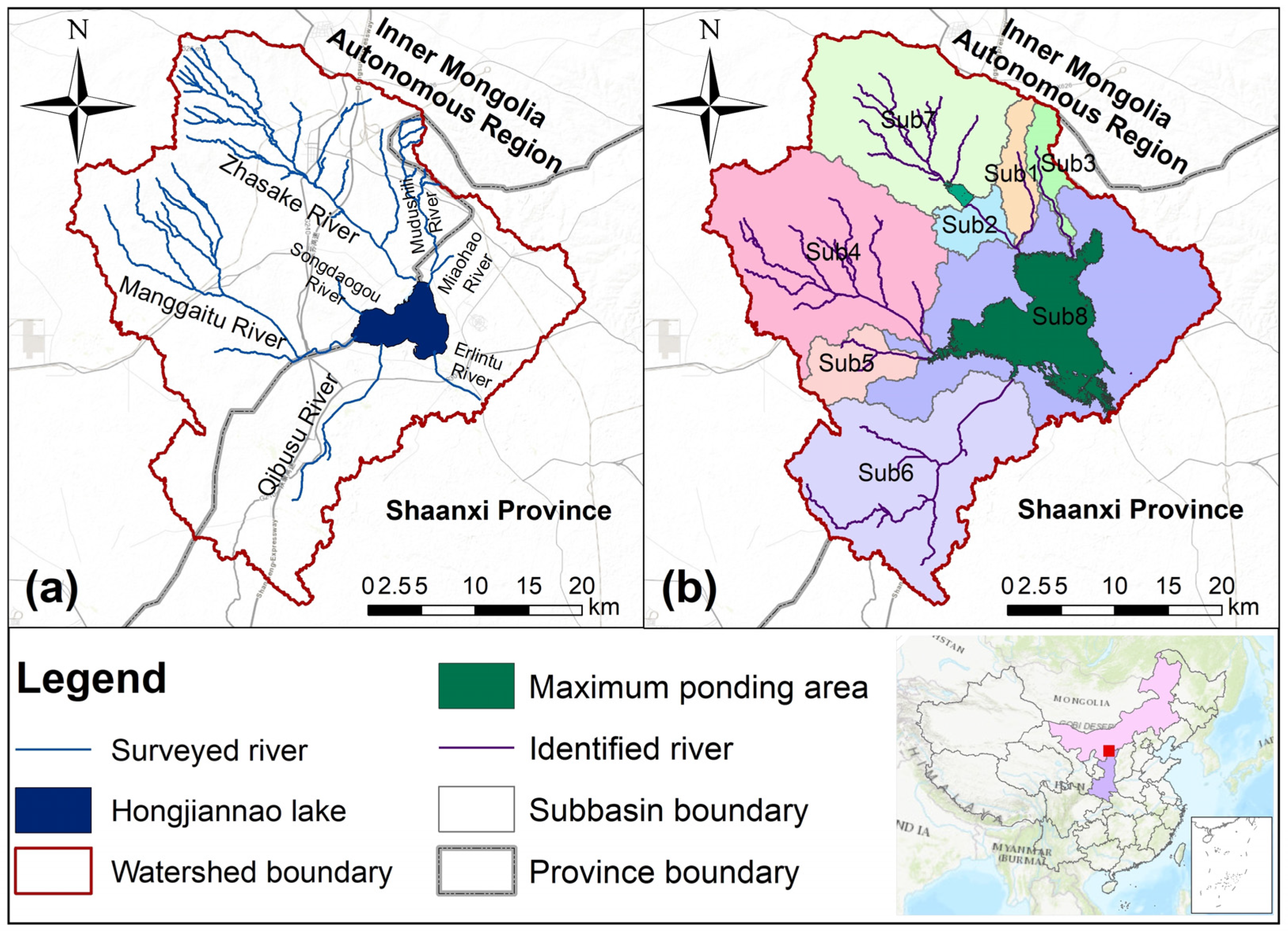
Figure 1. (a) Location of the Hongjiannao watershed and (b) surface delineation results (Sub = Subbasin).
Sustainability 15 06535 g001
Figure 2. Flowchart of the proposed approach.
Sustainability 15 06535 g002
Figure 3. Structures of (a) original HYDROL-DC and (b) modified HYDROL-DC (PBU = puddle-based unit; on-stream CBU = channel-based unit that has interaction with the main channel; off-stream CBU = channel-based unit that has no interaction with the main channel; CA = contributing area; and PA = ponding area).
Sustainability 15 06535 g003
Figure 4. Comparisons of the simulated and observed evapotranspiration of all sub-basins for the calibration period (1 January 2008–31 December 2013) and validation period (1 January 2014–31 December 2017).
Sustainability 15 06535 g004
Figure 5. Comparison of the simulated and observed areas of Hongjiannao Lake for (a) the calibration period (1 January 2008–31 December 2013) and (b) the validation period (1 January 2014–31 December 2017).
Sustainability 15 06535 g005
Figure 6. (a) Daily variations of rainfall and snowmelt, evaporation, and the storage of Hongjiannao Lake; (b) daily variations of contributing area inflow, upstream inflow, groundwater inflow, and the area of Hongjiannao Lake (RSIN = rainfall and snowmelt over the lake surface; EVA = evaporation from the lake surface; CAIN = inflow from the contributing area of Hongjiannao Lake; GWIN = inflow from the groundwater zone; USIN = inflow from the upstream rivers).
Sustainability 15 06535 g006
Figure 7. Annual water balance of HJN Lake (RSIN = rainfall and snowmelt over the lake surface; EVA = evaporation from the lake surface; CAIN = inflow from the contributing area of HJN Lake; GWIN = inflow from the groundwater zone; USIN = inflow from the upstream rivers).
Sustainability 15 06535 g007
Figure 8. Ratios of the annual inflows from different rivers to the annual upstream inflow of Hongjiannao Lake (ZSK = Zhasake; MGT = Manggaitu; MDSL = Mudushili; QBS = Qibosu).
Sustainability 15 06535 g008
Figure 9. The correlations between the storage variation of Hongjiannao Lake and the water balance terms in (a) the increase stage and (b) the decrease stage at the monthly time scale, and in (c) the increase stage and (d) the decrease stage at the daily time scale (RSIN = rainfall and snowmelt over the lake surface; EVA = evaporation from the lake surface; CAIN = inflow from the contributing area of Hongjiannao Lake; GWIN = inflow from the groundwater zone; USIN = inflow from the upstream rivers; DS = variation of lake storage).
Sustainability 15 06535 g009
Table 1. Major hydrologic processes simulated by HYDROL-DC (CA: contributing area; PA: ponding area; ET: evapotranspiration).
Zone NameHydrologic Processes
Canopy zone1. Interception
2. Evaporation
Snow zone1. Snow storage
2. Snow melt
3. Sublimination
Surface zone1. Surface runoff, infiltration, and runoff routing in CA
2. Percolation, evaporation, and runoff routing in PA
3. Variations of PA and its storage
Upper soil zone1. Soil temperature
2. Soil ET
3. Soil water content
4. Percolation to lower soil zone
Lower soil zone1. Percolation to groundwater zone
Shallow groundwater zone1. Percolation to deep groundwater zone
2. Discharge to main channels or lakes
Table 2. Major input data of HYDROL-DC.
Input DataSourceType
Topographic datahttps://www.eorc.jaxa.jp/ALOS/en/dataset/aw3d30/aw3d30_e.htm (accessed on 16 May 2022)Raster (30 m)
Precipitationhttp://data.tpdc.ac.cn/en/data/8028b944-daaa-4511-8769-965612652c49/ (accessed on 27 July 2022)Raster (0.1°)
Air temperaturehttp://www.glass.umd.edu/Download.html (accessed on 23 July 2022)Raster (250 m)
Leaf area indexhttp://www.glass.umd.edu/Download.html (accessed on 23 July 2022)Raster (250 m)
SCS curve numberhttps://figshare.com/articles/dataset/GCN250_global_curve_number_datasets_for_hydrologic_modeling_and_design/7756202 (accessed on 29 July 2022)Raster (250 m)
Soil datahttps://www.fao.org/soils-portal/data-hub/soil-maps-and-databases/harmonized-world-soil-database-v12/en/ (accessed on 11 August 2022)Raster (1 km)
Table 3. Area of HJN Lake from 2008 to 2017.
DateArea (km2)DateArea (km2)DateArea (km2)
24 April 200840.1624 September 201134.261 July 201531.40
10 May 200839.983 April 201334.2724 December 201530.72
15 September 200838.769 June 201332.739 January 201630.98
1 October 200839.3529 September 201333.0229 March 201631.87
21 January 200938.8416 November 201332.8916 May 201630.94
24 April 200939.7318 December 201332.9117 June 201630.62
29 May 200938.723 January 201432.8021 September 201634.03
30 June 200938.0520 February 201432.708 November 201635.32
20 October 200937.8227 May 201432.5910 December 201635.97
24 January 201037.9914 July 201431.8111 January 201736.34
20 August 201035.9315 August 201431.561 April 201736.08
8 November 201036.052 October 201431.9719 May 201735.88
10 December 201035.7521 December 201431.738 September 201734.52
27 January 201135.2623 February 201531.9626 October 201736.24
17 April 201136.1511 March 201532.13--
22 July 201134.8828 April 201532.61--
Table 4. Average annual surface runoff and consumptions of all sub-basins.
Sub-Basin IDArea (km2)Natural Surface Runoff (104 m3)Land Cover Change
(104 m3)
Climate Change
(104 m3)
Reservoir Construction
(104 m3)
Domestic
Usage
(104 m3)
Actual Surface Runoff
(104 m3)
133.95118.9416.8212.608.4913.2367.81
230.16105.6914.9511.197.5511.7660.25
327.40103.8313.5810.176.850.0073.21
4295.701031.42146.56109.7373.97217.58483.61
548.90170.5524.2318.1412.2335.9879.97
6267.831080.70132.7499.3867.00181.22600.44
7235.82826.32116.8887.5158.9991.94471.05
8404.031698.14200.25149.92101.07199.171110.38
Total1343.795135.59666.01498.64336.16750.892946.72
Table 5. Calibrated parameters and their sensitivity index values.
ParameterDescriptionsCalibration RangeCalibrated ValueSensitivity Index (I)
CcnpRatio of precipitation falling into canopy zone0–10.2−0.02
C1etEmpirical evapotranspiration parameters0–10.10.02
C2et0–10.10.05
C3et≥02.0−0.0001
CevaLake evaporation coefficient≥01.9−1.06
CNCurve number0–10065–741.16
IaInitial abstraction0–10.3−0.19
lagsurSurface runoff lag coefficient0–240.60.004
laglsSoil percolation lag coefficient (days)≥015–50 days−0.03
CsgwShallow groundwater percolation coefficient0–10.19–0.85−0.50
lagsgwShallow groundwater lag coefficient (days)≥010–200 days−0.01
Note: 0.00 ≤ |I| < 0.05: small to negligible sensitivity; 0.05 ≤ |I|< 0.20: medium sensitivity; 0.20 ≤ |I|< 1.00: high sensitivity; |I| ≥ 1.0: extremely sensitivity; a negative value of the index indicates the inverse impact of a parameter on the lake area [59].
Table 6. Comparisons of the simulated average annual surface runoff and the reference values of all sub-basins.
Sub-Basin IDAreaReference ValueSimulated ValueError
(km2)(104 m3)(mm)(104 m3)(mm)(%)
133.9567.8119.9873.1021.53+7.81
230.1660.2519.9866.0621.90+9.64
327.4073.2126.7274.7727.29+2.13
4295.70483.6116.35458.0315.49−5.29
548.9079.9716.3581.9816.77+2.52
6267.83600.4422.42601.0522.44+0.10
7235.82471.0519.98472.8220.05+0.37
8404.031110.3827.481005.4824.89−9.45
Table 7. Annual water balance table of Hongjiannao Lake (RSIN = rainfall and snowmelt over the lake surface; EVA = evaporation from the lake surface; CAIN = inflow from the contributing area of Hongjiannao Lake; GWIN = inflow from the groundwater zone; USIN = inflow from the upstream rivers; DS = lake storage variation).
YearSourceSinkDS
RSINCAINUSINGWINEVA
mm%mm%mm%mm%mm%mm
200841.9252.5416.4120.5618.2222.833.244.06153.86100.00−74.07
200924.9143.265.739.9414.2424.7212.7122.08144.63100.00−87.04
201026.2176.940.872.563.5710.483.4110.02127.82100.00−93.75
201124.8495.250.180.680.501.930.562.13118.05100.00−91.98
201241.8526.5345.4928.8457.0236.1613.358.4799.71100.0058.01
201332.1623.2125.8718.6750.5836.5029.9521.62126.69100.0011.87
201423.9746.182.905.6011.6622.4813.3625.75123.05100.00−71.15
201523.8239.9714.5124.3618.6631.322.594.35112.76100.00−53.17
201656.9517.20115.9335.02137.2341.4520.946.32106.28100.00224.76
201736.3421.1719.9311.6157.7133.6157.7133.61139.95100.0031.73
Disclaimer/Publisher’s Note: The statements, opinions and data contained in all publications are solely those of the individual author(s) and contributor(s) and not of MDPI and/or the editor(s). MDPI and/or the editor(s) disclaim responsibility for any injury to people or property resulting from any ideas, methods, instructions or products referred to in the content.