Spatial Distribution of Soil Water and Salt in a Slightly Salinized Farmland

Abstract

It is important to study the mechanisms associated with the spatial distribution of soil water and salt to control soil salinization and promote the sustainable development of farmland. Six plots in a slight farmland with different spatial locations were selected to determine the spatial distribution of soil water and salt and their correlation using the multifractal method. Each plot was applied using the grid method (15 m × 15 m, 3600 m²), where each sampling site was located at the center point coordinates. The 0–20 and 20–40 cm soil layers were sampled.The spatial variability of the soil water and salt were 1.41 and 1.73 fold higher in the upstream farmland than in the downstream farmland. The spatial variability of the soil water and salt was significantly correlated. In addition, the spatial variability of the soil water and salt significantly correlated in the 0–20 and 20–40 cm layers. The spatial distribution of both soil water and salt in the entire soil layer had similar characteristics at this sampling scale. Our results provide a theoretical basis to study the interactive mechanisms associated with the distribution of soil water and salt.

1. Introduction

Soil salt is a significant factor that affects crop growth [1,2]. The accumulation of salt in soil leads to salinization, thereby resulting in land degradation and even damage to the ecological environment [3,4,5]. Therefore, determining the spatial distribution of soil salt is very important to prevent and control salinization. The spatial distribution of soil salt is affected by many factors, such as rainfall, groundwater, and soil properties, among others, etc. [6,7,8,9]. In particular, the influence of soil water on the distribution of salt is the most important factor [10,11]. The soil water carries salt, which facilitates its migration, and thus the spatial distribution of water determines the spatial distribution of salt to a great extent [12,13]. However, the relative humidity in soil pores decreases as the salt dissolves in liquid water, and the reduced pore volume affects the transport of soil water [14]. Therefore, it is assumed that the spatial distribution of soil water and salt will be correlated because of their coupling.

The spatial distribution of soil water and salt has been studied extensively. In particular, Yuan et al. [15] described the distribution of soil water based on the classical statistical method, but this method did not consider the spatial distribution characteristics. Benslama et al. [16] and Liu et al. [17] applied geostatistics to determine the spatial distribution characteristics of soil salt and optimize the sampling scale in saline and alkaline areas. Zhao et al. [18] showed that the Granger–Ramanathan averaging weights could be adopted as a protocol to predict district-scale clay prediction. However, Wang et al. [19] showed that geostatistics have some disadvantages when quantifying the local spatial variability of some properties because geostatistical theory only reflects the variability of the soil properties based on a value calculated using a function, and thus the detailed spatial variability of the soil properties cannot be characterized with this method. Liao et al. [20] compared the spatial variability of the soil moisture at different sampling stages in two adjacent land use types with the single fractal method, but the use of only one parameter (fractal dimension) cannot represent sufficient information regarding the spatial variability. However, the calculation of multifractal parameters calculated using multifractal theory can describe the characteristic spatial distribution in detail [21]. Therefore, in recent years, the multifractal method has been used widely to study the spatial distribution of soil properties. Wang et al. [22] showed that multifractal parameters could quantify the spatial variability of the soil particle size distribution range, concentration degree, non-uniformity, and non-symmetry. Xia et al. [23] studied the multifractal characteristics of the soil particle distribution under different vegetation types and showed that the roughness and inhomogeneity of the soil particles in shrub communities were significantly lower than those in bare land. Wang et al. [19] evaluated the effects of open-pit mining and related soil discharge activities on the nature of reconstructed soil and showed that the local and total variability of the soil organic matter, total nitrogen (TN), and total phosphorus were higher in the 20–40 cm layer than the 0–20 cm layer. Thus, the multifractal method may perform better at determining the spatial distribution of soil water and salt.

Optimization of the soil sampling scheme can reduce the sampling cost, and this problem has primarily been addressed in previous studies by using geostatistics in previous studies [24]. Wang and Shao [25] showed that a sampling interval of 100 m was adequate to detect the spatial structure of four soil physical properties, including saturated hydraulic conductivity, total porosity, capillary porosity, and bulk density within a watershed. Wu et al. [26] used the kriging method to explore the relationship between the soil organic carbon (C) and landscape index depending on the sampling scale and showed that a sampling interval of 300 m was the optimal scale. Their results indicated that geostatistics could not directly characterize the correlations in the spatial variability between variables [19]. In addition, Zhao et al. [27] predicted the soil’s physical and chemical properties using Visible-Near Infrared (Vis-NIR) spectroscopy in Australian cotton areas and showed that multi-depth bagging-partial least squares regression (PLSR) was superior. Overall, a multi-depth spectral library is recommended for Vertosols. The joint multifractal method can be used to characterize the correlations between the spatial distribution of two or more variables. Indeed, Wang et al. [19] utilized the joint multifractal method to show that the distribution of the sand, organic matter, and TN highly spatially correlated in the 0–20 and 20–40 soil layers, whereas the distribution of the clay and silt contents had weak spatial correlations. Bertol et al. [28] also used the joint multifractal method and found that the relationship between soil and water loss depended on the scale of the study scale, and their respective scale indices differed in terms of their degrees of correlation degrees under different tillage treatments. These studies demonstrate that the joint multifractal method can characterize the correlations among the spatial distribution of soil properties in different soil layers. Therefore, we considered that the joint multifractal method could potentially be applied to determine the correlation between the spatial distribution of soil water and salt.

The spatial distributions of the soil water and salt have been widely investigated in previous studies, but the correlations in their spatial distributions have not been considered. Therefore, in the present study, our objectives in this study were as follows: (1) to determine the characteristic spatial distribution of the soil water and salt; (2) to evaluate the correlations between the spatial distribution of soil water and salt; and (3) to optimize the soil water and salt sampling scheme.

2. Materials and Methods

2.1. Description of the Study Area

The experimental site was located in Nangou Village, Yanan City, Shaanxi Province, north China (40°14′11″ N to 42°27′42″ N, 75°33′16″ E to 80°59′7″ E). The site is located in gully farmland in the Loess Hilly Region of China, with an average elevation of 1371.9 m, mean annual precipitation of 505.3 mm, mean annual temperature of 8.6 °C, mean annual total sunshine duration of 2395.6 h, mean annual total radiation of 493 kJ cm⁻², and mean annual potential evaporation of 1463 mm [29,30,31,32]. The experimental plot was prepared in farmland planted with alfalfa (Medicago sativa Linn.). The soil meets the standard to be considered slightly saline soil. The soil pH was 7.9, the organic C content was 15.90 g kg⁻¹, the TN content was 0.91 g kg⁻¹, and the C:N was 17.7:1. The other basic soil properties in the different soil layers are shown in

Table 1. Soil basic properties in the experimental site.

Soil Layers (cm)	Bulk Density (g cm−3)	Field Capacity (%)	Saturated Hydraulic Conductivity (cm min−1)	Clay (0~0.002 mm) %	Silt (0.002~0.02 mm) %	Sand (0.02~2 mm) %	Soil Texture
0–20	1.17	24.80	0.57	9.85	39.20	50.96	Loam
20–40	1.26	25.00	0.36	9.99	40.04	49.97	Loam

.

The farm that was formed in a small watershed was divided into upstream and downstream farmland areas. The upstream farmland comprised plots 1–3, and the downstream farmland comprised plots 4–6 (Figure 1). The upstream and downstream farmland areas covered 3.5 ha and 12.8 ha, respectively. A drainage ditch was present on the south side of the farmland, but no drainage facilities were installed on the north side. Four gullies on the north slope of the farmland were labeled as gullies 1–4, respectively. The runoff from gully 4 was drained by the drainage ditch between plots 4 and plot 5 (Figure 1). The was 1.13 g kg⁻¹ of soluble salt in the sediment from the gully.

2.2. Experimental Design and Soil Sample Measurements

The soil water and salt contents can vary among the seasons [33,34], and they are susceptible to external factors, particularly rainfall, groundwater, and evapotranspiration [35,36]. Soil salt primarily accumulates during high periods of evaporation [2], and it is affected by rainfall. Thus, the period of high evaporation and drought period is the optimal choice to monitor the condition of soil salt. In this study, soil samples were collected from 8 to 10 July 2020. Six experimental plots were selected in different spatial locations (Figure 1) to determine the spatial distribution of the soil water and salt and their correlations. Plots 1, 2, and 3 were defined as upstream, and plots 4, 5, and 6 were defined as downstream. Each plot had an area of 3600 m². A grid method was utilized (15 m × 15 m) where each sampling site was located at the center of the point coordinates by using a tape measure (Figure 2). Soil samples were obtained using a soil auger (4 cm in diameter, with a retractable extended drill stem) from the 0–20 and 20–40 cm layers. Each hole was backfilled with soil after sampling.

The soil samples were dried to a constant weight at 105 °C to determine the soil water content. The soluble salt content was determined using the gravimetric method [37]. The soil electrical conductivity (EC) was determined using an EC meter (DDS-307A, Shanghai Yidian Scientific Instrument Co., Ltd., Shanghai, China) after the soil samples were first air dried, passed through a 2 mm sieve, and mixed uniformly [37]. Next, the samples were placed into distilled water in a sealed plastic bottle at a ratio of 1:5, shaken for 30 min, allowed to settle, and measured twice with an EC meter. The fitted equation between the soluble salt content and EC was as follows: soluble salt content (g kg⁻¹) = 0.0042EC (μs cm⁻¹) − 0.1032 (n = 40, p < 0.01) [30]. The EC values were then converted into the soluble salt contents. The methods used to determine the bulk density, field capacity, and saturated hydraulic conductivity were conducted as described by the experimental methods for soil and water conservation. The soil particle size was determined by laser diffraction analysis (Mastersizer 2000, Malvern Panalytical, Ltd., Malvern, UK) [31].

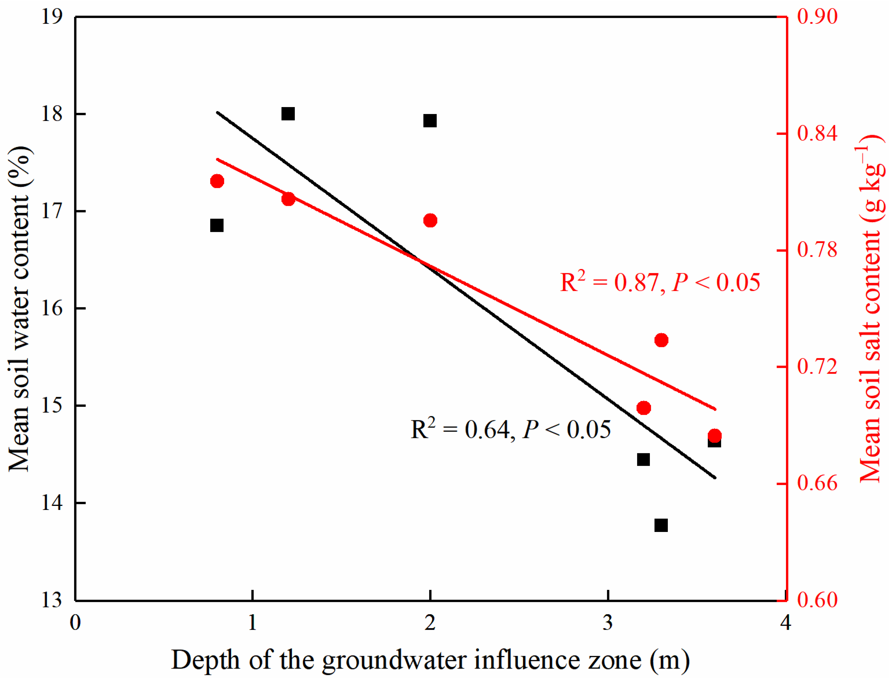
2.3. Depth of the Groundwater Influence Zone

The depth of the groundwater influence zone was determined for each plot. An auger (4 cm in diameter) was used to extract the soil cores. When a soil core was obviously water-saturated, it was considered that the groundwater influence zone was considered to have been reached, and the depth from the soil surface down to this layer was recorded [29]. The depths determined for the groundwater influence zones are shown in Figure 3. The average depths of the groundwater influence zones in the upstream and downstream farmland areas were 1.33 m and 3.67 m, respectively. The depth of the groundwater influence zone was negatively correlated with the soil water and salt (p < 0.05). Jin et al. [29] showed that the content of soil salt in the groundwater was 450 mg L⁻¹ in the study area.

2.4. Fractal Methods

2.4.1. Multifractal Analysis

The spatial distributions of the soil water and salt were analyzed using the multifractal method. A square grid measuring ε covered by part of the space was used to calculate the generalized dimension Dq [38]. In each plot, N (ε) = 2^k (k = 0, 1, 2, …) cells were considered [39]. The six plots measured 60 m × 60 m, and the size of each sampling point was 15 m × 15 m, so four grid side lengths comprising 15 m, 20 m, 30 m, and 60 m were considered in this study, where the total numbers of grids in each plot were 16, 9, 4, and 1, respectively (Figure 2).

The probability mass function (${\mathrm{p}}_{\mathrm{i}}\left(\mathsf{\epsilon }\right))$ was computed as follows [38]:

$${\mathrm{p}}_{\mathrm{i}}\left(\mathsf{\epsilon }\right)=\frac{{\mathrm{Z}}_{\mathrm{i}}}{{\sum }_{\mathrm{i}=1}^{\mathrm{N}\left(\mathsf{\epsilon }\right)}{\mathrm{Z}}_{\mathrm{i}}}$$

(1)

where ${\mathrm{Z}}_{\mathrm{i}}$ is the value for a given size of ε and N (ε) is the number of grids.

D_q is defined as follows:

$${\mathrm{D}}_{\mathrm{q}}=\underset{\mathsf{\epsilon }\to 0}{\lim }\frac{1}{\mathrm{q}-1}\times \frac{\lg ({\sum }_{\mathrm{i}=1}^{\mathrm{N}\left(\mathsf{\epsilon }\right)}{{\mathrm{p}}_{\mathrm{i}}\left(\mathsf{\epsilon }\right)}^{\mathrm{q}})}{\lg \mathsf{\epsilon }}\left(\mathrm{q}\ne 1\right),\mathrm{a}\mathrm{n}\mathrm{d}$$

(2)

$${\mathrm{D}}_1=\underset{\mathsf{\epsilon }\to 0}{\mathrm{l}\mathrm{i}\mathrm{m}}\times \frac{{\sum }_{\mathrm{i}=1}^{\mathrm{N}\left(\mathsf{\epsilon }\right)}{\mathrm{p}}_{\mathrm{i}}\left(\mathsf{\epsilon }\right)\lg {\mathrm{p}}_{\mathrm{i}}\left(\mathsf{\epsilon }\right)}{\lg \mathsf{\epsilon }}\left(\mathrm{q}=1\right),$$

(3)

where q represents integers in (+∞, −∞), i.e., the probability density weight index [40]. D₁ is the information dimension. A high D₁ value indicates that the soil water and salt values are distributed over a relatively large domain, and they exhibit relatively low spatial variability, whereas a low D₁ value indicates that the soil water and salt values are concentrated over a relatively small domain with relatively high spatial variability [38]. ΔD (D₋₁₀ − D₁₀) can reflect the degree of spatial variability of the soil water and salt in a local distribution, where a higher ΔD value indicates greater variability [41,42].

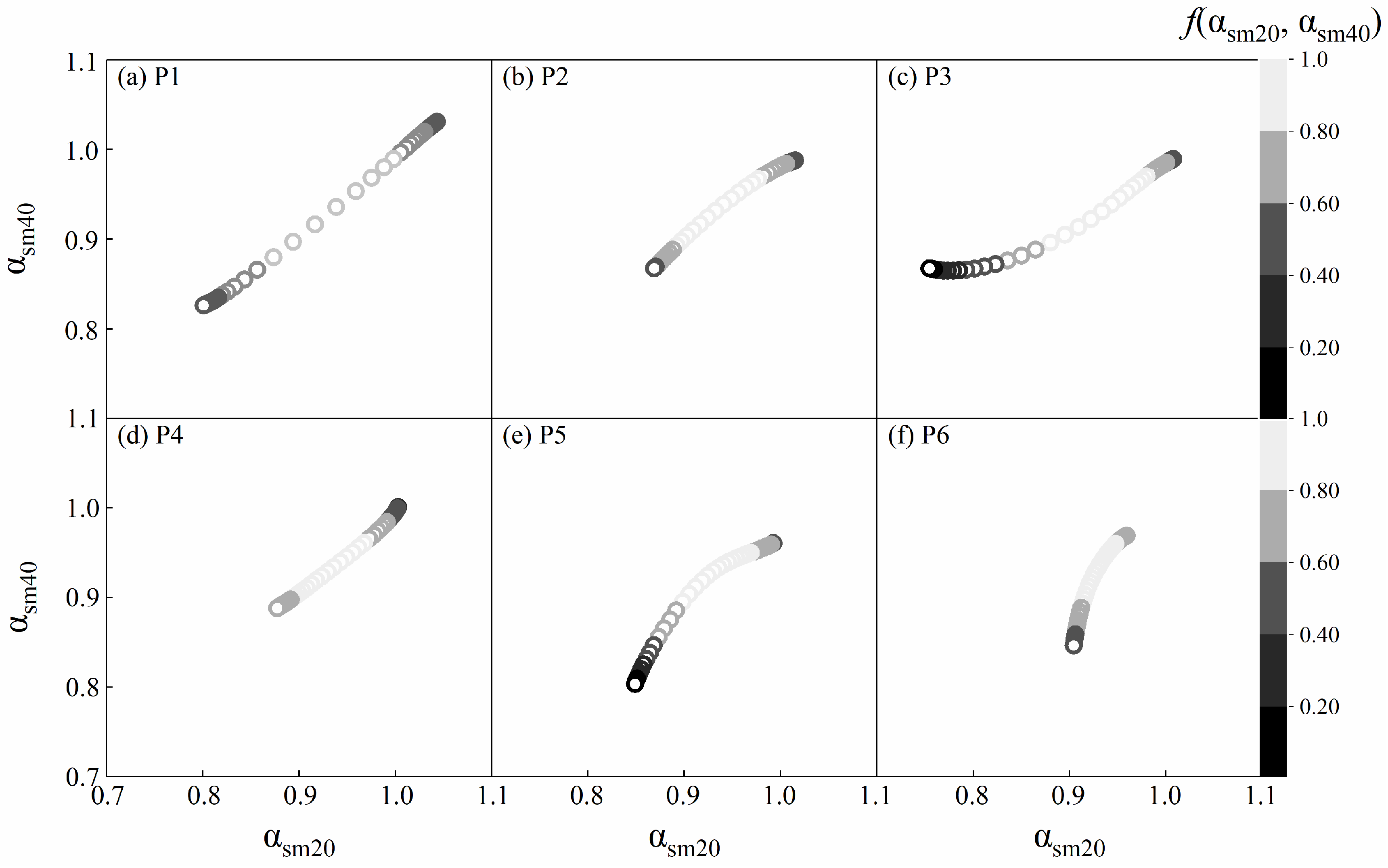
2.4.2. Joint Multifractal Analysis

The correlations between the spatial distributions of the soil water and salt were analyzed using the joint multifractal method. The normalized joint partition function: ${\mathsf{\mu }}_{\mathrm{i}}$ = (q¹, q², ε), was calculated as follows:

$${\mathsf{\mu }}_{\mathrm{i}}=({\mathrm{q}}^1,{\mathrm{q}}^2,\mathsf{\epsilon })=\frac{{\mathrm{p}}_{\mathrm{i}}^1{\left(\mathsf{\epsilon }\right)}^{{\mathrm{q}}^1}{\mathrm{p}}_{\mathrm{i}}^2{\left(\mathsf{\epsilon }\right)}^{{\mathrm{q}}^2}}{{\sum }_{\mathrm{i}=1}^{\mathrm{N}\left(\mathsf{\epsilon }\right)}{\mathrm{p}}_{\mathrm{i}}^1{\left(\mathsf{\epsilon }\right)}^{{\mathrm{q}}^1}{\mathrm{p}}_{\mathrm{i}}^2{\left(\mathsf{\epsilon }\right)}^{{\mathrm{q}}^2}},$$

(4)

where N($\mathsf{\epsilon }$) indicates the interval when the scale is $\mathsf{\epsilon }$, q¹ and q² are the moment orders of soil water and salt, respectively, and ${\mathrm{p}}_{\mathrm{i}}^1\left(\mathsf{\epsilon }\right)$ and ${\mathrm{p}}_{\mathrm{i}}^2\left(\mathsf{\epsilon }\right)$ are the normalized probability mass functions for the soil water and salt [19].

The Hólder exponents of the soil water and salt were calculated as follows [40]:

$${\mathsf{\alpha }}_1\left({\mathrm{q}}^1,{\mathrm{q}}^2\right)=-\frac{{\sum }_{\mathrm{i}=1}^{\mathrm{N}\left(\mathsf{\epsilon }\right)}\left[{\mathsf{\mu }}_{\mathrm{i}}\left({\mathrm{q}}^1,{\mathrm{q}}^2,\mathsf{\epsilon }\right)\mathrm{l}\mathrm{g}{\mathrm{p}}_{\mathrm{i}}^1\left(\mathsf{\epsilon }\right)\right]}{\mathrm{l}\mathrm{g}\mathrm{N}\left(\mathsf{\epsilon }\right)},\mathrm{a}\mathrm{n}\mathrm{d}$$

(5)

$${\mathsf{\alpha }}_2\left({\mathrm{q}}^1,{\mathrm{q}}^2\right)=-\frac{{\sum }_{\mathrm{i}=1}^{\mathrm{N}(\mathsf{\epsilon })}\left[{\mathsf{\mu }}_{\mathrm{i}}\left({\mathrm{q}}^1,{\mathrm{q}}^2,\mathsf{\epsilon }\right)\lg {\mathrm{p}}_{\mathrm{i}}^2\right(\mathsf{\epsilon }\left)\right]}{\lg \mathrm{N}(\mathsf{\epsilon })},$$

(6)

where α₁ and α₂ are the Hólder exponents for the soil water and salt, respectively, and:

$$f\left({\mathsf{\alpha }}_1,{\mathsf{\alpha }}_2\right)=-\frac{{\sum }_{\mathrm{i}=1}^{\mathrm{N}(\mathsf{\epsilon })}\left[{\mathsf{\mu }}_{\mathrm{i}}\left({\mathrm{q}}^1,{\mathrm{q}}^2,\mathsf{\epsilon }\right)\lg {\mathsf{\mu }}_{\mathrm{i}}\left({\mathrm{q}}^1,{\mathrm{q}}^2,\mathsf{\epsilon }\right)\right]}{\lg \mathrm{N}\left(\mathsf{\epsilon }\right)},$$

(7)

where the dimension f(α₁, α₂) represents a set in which α₁ and α₂ represent the mean local exponents for the soil water and salt, respectively [19].

The image composed of ${\mathsf{\alpha }}_1\left({\mathrm{q}}^1,{\mathrm{q}}^2\right)$, ${\mathsf{\alpha }}_2\left({\mathrm{q}}^1,{\mathrm{q}}^2\right)$, and $f\left({\mathsf{\alpha }}_1,{\mathsf{\alpha }}_2\right)$ is the joint multifractal spectrum. The correlation between the soil water and salt can be qualitatively described based on the shape of the grayscale. Increases in the extension and concentration of a grayscale image along a diagonal line denote a stronger correlation between the soil water and salt. Conversely, a low spatial dependency between the soil water and salt is indicated if the distribution of the grayscale values in the image is discrete [19,43].

2.5. Statistical Analysis

The values calculated for soil water and salt were analyzed using classical statistical methods. We used SPSS 23.0 (IBM, Inc., Armonk, NY, USA) to calculate Pearson’s correlation coefficients and to fit the relationships among the depth of the groundwater influence zone, soil water content, and salt content. The spatial distributions of soil water and salt were analyzed using the multifractal method. The correlations between the spatial distribution of the soil water and salt were analyzed using the joint multifractal method. The graphs were prepared using Origin Pro 8.0 (OriginLab, Northampton, MA, USA).

3. Results

3.1. Descriptive Statistics for Soil Water and Salt

The descriptive statistics obtained for soil water and salt in the 0–20 cm and 20–40 cm layers in each plot are shown in

Table 2. Mean soil water and salt contents in each plot.

Soil Properties	Soil Layers (cm)	Upstream			Downstream
		Plot 1	Plot 2	Plot 3	Plot 4	Plot 5	Plot 6
Soil water	0–20	15.80	17.07	16.85	12.62	13.63	13.24
content (%)	20–40	17.79	18.94	19.01	14.91	15.27	16.04
	Mean	16.79	18.00	17.93	13.77	14.45	14.64
Soil salt	0–20	0.90	0.84	0.81	0.75	0.73	0.72
content (g kg−1)	20–40	0.74	0.77	0.78	0.72	0.67	0.65
	Mean	0.82	0.81	0.80	0.73	0.70	0.68

. The average soil water contents in the complete layer from plots 1 to 6 were 16.85, 18.00, 17.93, 13.77, 13.94, and 14.64%, respectively, and the mean soil salt contents were 0.82, 0.81, 0.80, 0.73, 0.70, and 0.68 g k⁻¹. The average soil water and salt contents in the upstream farmland were 17.59% and 0.81 g kg⁻¹, which were 23.15% and 15.17% higher than those in the downstream farmland, respectively, and similar results were reported by Jin et al. [29]. The following two possible reasons could explain these results. (i) The average depths of the groundwater influence zones were 1.33 and 3.67 m in the upstream and downstream farmland areas, respectively. The depth of the groundwater influence zone had significant negative correlations with the soil water and salt content (p < 0.05) (Figure 3). A high groundwater influence zone depth will increase the groundwater level, which results in the movement of salt into the surface soil [2]. (ii) Compared with the downstream farmland area, runoff and sediment from gullies with high salt contents intruded into the upstream farmland area (Figure 1), thereby increasing the water and salt contents in the upstream farmland area.

3.2. Spatial Distribution of Soil Water and Salt

The generalized dimension spectra obtained for the soil water and salt between the 0–20 cm and 20–40 cm layers in each plot are shown in Figure 4 and Figure 5, respectively. The D(q) values decreased as the q values increased, thereby indicating that the soil water and salt exhibited multifractal characteristics in the complete soil layer in all the plots [44].

Table 3. Multifractal parameters determined for soil water and salt in each plot.

Soil Properties	Soil Layers (cm)	Multifractal Parameters	Upstream Farmland				Downstream Farmland
			Plot 1	Plot 2	Plot 3	Mean	Plot 4	Plot 5	Plot 6	Mean
Soil water	0–20	D1	1.9694	1.9610	1.9579	1.9628	1.9772	1.9740	1.9846	1.9786
		ΔD	0.1929	0.4208	0.5421	0.3853	0.1969	0.2440	0.0774	0.1728
	20–40	D1	1.9791	1.9789	1.9743	1.9774	1.9800	1.9768	1.9754	1.9774
		ΔD	0.1051	0.1594	0.2214	0.1620	0.1601	0.2523	0.2366	0.2163
Soil salt	0–20	D1	1.9817	1.9796	1.9842	1.9818	1.9852	1.9848	1.9857	1.9852
		ΔD	0.1655	0.1593	0.0927	0.1392	0.0689	0.0620	0.0711	0.0673
	20–40	D1	1.9849	1.9811	1.9829	1.9830	1.9839	1.9855	1.9849	1.9848
		ΔD	0.1300	0.1397	0.1499	0.1399	0.0829	0.0540	0.0659	0.0676

shows that the average D₁ value in soil water was less for the upstream farmland (1.9701) than the downstream farmland (1.9780), and the average ΔD value was 1.41-fold higher for upstream farmland than downstream farmland in the whole layer. Similar results were found for soil salt in the entire soil layer. The average D₁ value was less for the upstream farmland (1.9824) than the downstream farmland (1.9850), and the average ΔD value was 1.73-fold higher for the upstream farmland than the downstream farmland. These results indicate that the spatial variability of the soil water and salt were higher in the upstream farmland than in the downstream farmland. In most cases, the spatial variability of the soil water and salt was higher in the 0–20 cm layer than in the 20–40 cm layer.

3.3. Correlations between Soil Water and Salt in the Same Layer

Figure 6 shows that the soil salt contents in the 0–20 cm and 20–40 cm layers were significantly correlated in all the plots (p < 0.05). Similarly, the soil water contents were also significantly correlated, except in plot 2 (p < 0.05). Grayscale images of the joint multifractal spectra obtained for the soil water and salt in the 0–20 cm and 20–40 cm layers are shown in Figure 7 and Figure 8, respectively. The α_sm20, α_ss20, and f(α_sm20, α_ss20) values represent the singularity index for soil water, the singularity index for soil salt, and the joint dimension distribution function for soil water and salt, respectively, in the 0–20 cm layer. The α_sm40, α_ss40, and f(α_sm40, α_ss40) values represent the singularity index for soil water, singularity index for soil salt, and the joint dimension distribution function for soil water and salt, respectively, in the 20–40 cm soil layer. The grayscale images are diagonal and concentrated in Figure 7 and Figure 8, thereby indicating that the spatial variability of the soil water and salt were highly correlated in the entire layer in all the plots.

3.4. Correlations between Soil Water and Salt in the 0–20 cm and 20–40 cm Soil Layers

Grayscale images of the joint multifractal spectra obtained for soil water and salt in the 0–20 cm and 20–40 cm layers are shown in Figure 9 and Figure 10, respectively. The f(α_sm20, α_sm40) and f(α_ss20, α_ss40) values represent the joint dimension distribution functions for soil water and salt in the 0–20 cm and 20–40 cm layers, respectively. The spatial distribution of soil water and salt were highly correlated in the 0–20 cm and 20–40 cm layers, thereby indicating that the characteristic spatial distribution of soil water and salt in the complete layer could be represented by those in the 0–20 cm layer.

4. Discussion

4.1. Spatial Variability of Soil Water and Salt

The spatial distributions of soil water and salt are owing to dynamic processes [45]. In this study, we analyzed the distribution of soil water and salt in six plots with different spatial locations. We found that the spatial variability of the soil water and salt was higher in the upstream farmland areas than that in the downstream farmland areas (Table 3, Figure 4 and Figure 5), which may be explained as follows. (i) The upstream farmland was affected by runoff and sediment, and the soil-soluble salt content of the sediment was 1.13 g kg⁻¹. The topsoil of the sloping farmland was eroded and invaded the upstream farmland through northern gullies 1–3 after heavy rainfall (Figure 1). The uneven runoff and sediment distribution increased the spatial variability of soil water and salt. However, the runoff and sediment from gully 4 in the downstream farmland were discharged by the drainage facilities between plots 4 and 5, thereby indicating that the downstream farmland was generally unaffected. (ii) Landform features in the upstream farmland had important effects on the spatial variability of soil water and salt. The upstream farmland was narrow, whereas the downstream farmland was wider. The area of the upstream farmland was only 0.27-fold times that of the downstream farmland (Figure 1). Thus, the vulnerability of the upstream farmland to waterlogging caused the spatial variability of the soil water and salt. (iii) Fang et al. [46] reported that the spatial variability of soil water was higher when the soil water content was higher. In this study, the soil water content was 23.0% higher in the upstream farmland than in the downstream farmland (Table 2), which is consistent with the results obtained by Fang et al. [46]. In most cases, the spatial variability of soil water and salt was higher in the 0–20 cm layer than in the 20–40 cm layer. Similar results were obtained in arid and semiarid saline areas by Cao et al. [47] and Dong et al. [2]. These differences can primarily be explained by the greater vulnerability of the 0–20 cm soil layer to the effects of external factors, such as rainfall, evapotranspiration, and vegetation cover [48].

4.2. Correlations between the Spatial Variability of Soil Water and Salt

The correlations between the spatial variability of the soil water and salt were high in the whole soil layer in all the plots (p < 0.05) (Figure 6, Figure 7 and Figure 8), thereby indicating that the results were not affected by the experimental site, depth of the groundwater table, and soil layers. The correlations can primarily be explained by the coupling between soil water and salt. The soil pores in arid and semiarid areas, the soil pores usually contain air, liquid soil water, and salt. The movement of soil water is responsible for the migration of salt, and thus the spatial distribution of water primarily determines that of salt. However, the relative humidity of the pores decreases as the salt dissolves in liquid water and the pore volume is reduced, which thereby affects the transport of soil water and even its distribution [14]. Wen et al. [14] verified the existence of water–salt coupling based on a model developed based on film water transport theory, which considered the influence of salt on surface tension as well as the filling effect of precipitated salt on the soil pores, residual volumetric air content, the effect of salt on heat transport and storage, and the influences of vapor flux and thermal radiation on the thermal boundary. Li et al. [49] also proposed a new uncertainty simulation optimization framework for the distribution of irrigation water distribution based on the physical water–salt coupling process, where this framework focused on the effects of soil water and salt migration on the distribution of irrigation water in the field. These previous studies demonstrated the coupling of water and salt in soil.

In this study, the range of the soil water content was 12.6~19.0% (Table 2). Thus, most of the soil salt was dissolved in water. We predict that the correlation between the spatial variability of soil water and salt will decrease when the soil water content is lower because soil salt may be precipitated, and the solid crystals would block the capillary pores in the soil layer [50]. Therefore, the correlations between the spatial variability of soil water and salt should be investigated under a wider range of water contents in future research.

4.3. Optimization of Soil Water and Salt Sampling

Based on the spatial autocorrelation of soil properties, the sampling scale and samples can be estimated with a certain sampling accuracy [51]. Many previous studies have aimed to determine the optimal sampling scale or sample number by using geostatistical methods. For example, Wang et al. [52] employed geostatistical analysis to optimize the soil TN and organic C contents in a mining area, and the optimal number of sample points was determined as 40 at the research scale considered. Domenech et al. [53] used the improved kriging method to determine an independent validation dataset based on sampling from a 30 m grid and found that 50% of the samples were sufficient to verify the most realistic estimation of the accuracy. Their results indicate that the sampling scale and the number of samples were only estimated in a single soil layer. In this study, we found that the spatial variability of the soil water and salt were highly correlated in the 0–20 cm and 20–40 cm layers in the plots (p < 0.05) (Figure 8, Figure 9 and Figure 10), thereby indicating that the spatial distribution of the soil and salt in the entire layer can be obtained by only analyzing those in the 0–20 cm layer. Similarly, Wang et al. [19] used the joint multifractal method to show that the spatial distribution of the contents of sand, organic matter, and total nitrogen contents in the whole soil could be represented by that in the 0–20 cm layer and recommended using the 0–20 cm layer as the sampling layer in mining soil. These results indicate that the soil water and salt in the 0–40 cm layer were spatially autocorrelated at our sampling scale in the study region. Both geostatistical and joint multifractal methods can optimize the sampling scheme based on different dimensions. Therefore, we suggest that these two optimization strategies should be combined in future studies to substantially reduce the number of soil samples required.

5. Conclusions

In this study, the spatial distribution of soil water and salt and their correlations were analyzed using multifractal and joint multifractal methods in different spatial locations. The spatial variability of soil water and salt were higher in the upstream farmland than in the downstream farmland. Landform features and slope runoff sediment were the primary factors that were responsible for the differences. Compared with the downstream farmland, the Landform features of the upstream farmland were narrow. Moreover, the upstream farmland was affected by runoff and sediment, which increased the spatial variability of soil water and salt. The coupling between soil water and salt explained the high correlations between the spatial distribution of soil water and salt. In addition, the spatial distribution of soil water and salt in the whole layer was represented by that in the 0–20 cm layer because of the spatial autocorrelations of the soil properties, thereby indicating that the 0–20 cm layer could be used to monitor the soil water and salt in the study area. Our results provide new insights into the spatial distribution of soil water and salt and provide a new theoretical basis to optimize soil water and salt sampling schemes.

References

1. Butcher, K.; Wick, A.F.; Desutter, T.; Chatterjee, A.; Harmon, J. Soil Salinity: A Threat to Global Food Security. Agron. J. 2016, 108, 2189. [Google Scholar] [CrossRef]
2. Dong, Q.; Yang, Y.; Zhang, T.; Zhou, L.; He, J.; Chau, H.W.; Zou, Y.; Feng, H. Impacts of ridge with plastic mulch-furrow irrigation on soil salinity, spring maize yield and water use efficiency in an arid saline area. Agric. Water Manag. 2018, 201, 268–277. [Google Scholar] [CrossRef]
3. Akça, E.; Aydin, M.; Kapur, S.; Kume, T.; Nagano, T.; Watanabe, T.; Çilek, A.; Zorlu, K. Long-term monitoring of soil salinity in a semi-arid environment of Turkey. CATENA 2020, 193, 104614. [Google Scholar] [CrossRef]
4. Litalien, A.; Zeeb, B. Curing the earth: A review of anthropogenic soil salinization and plant-based strategies for sustainable mitigation. Sci. Total Environ. 2020, 698, 134235. [Google Scholar] [CrossRef] [PubMed]
5. Wang, Y.; Deng, C.; Liu, Y.; Niu, Z.; Li, Y. Identifying change in spatial accumulation of soil salinity in an inland river watershed, China. Sci. Total Environ. 2018, 621, 177–185. [Google Scholar] [CrossRef] [PubMed]
6. Jiang, X.; Ma, Y.; Li, G.; Huang, W.; Zhao, H.; Cao, G.; Wang, A. Spatial Distribution Characteristics of Soil Salt Ions in Tumushuke City, Xinjiang. Sustainability 2022, 14, 16486. [Google Scholar] [CrossRef]
7. Liu, W.Q.; Lu, F.; Xu, X.; Chen, G.; Fu, T.; Su, Q. Spatial and Temporal Variation of Soil Salinity during Dry and Wet Seasons in the Southern Coastal Area of Laizhou Bay, China. Indian J. Geo-Mar. Sci. 2020, 49, 260–270. [Google Scholar]
8. Tan, X.; Wu, M.; Huang, J.; Wu, J.; Chen, J. Similarity of soil freezing characteristic and soil water characteristic: Application in saline frozen soil hydraulic properties prediction. Cold Reg. Sci. Technol. 2020, 173, 102876. [Google Scholar] [CrossRef]
9. Zhang, J.; Lai, Y.; Li, J.; Zhao, Y. Study on the influence of hydro-thermal-salt-mechanical interaction in saturated frozen sulfate saline soil based on crystallization kinetics. Int. J. Heat Mass Transf. 2020, 146, 118868. [Google Scholar] [CrossRef]
10. Mainuddin, M.; Maniruzzaman, M.; Gaydon, D.; Sarkar, S.; Rahman, M.; Sarangi, S.; Sarker, K.; Kirby, J. A water and salt balance model for the polders and islands in the Ganges delta. J. Hydrol. 2020, 587, 125008. [Google Scholar] [CrossRef]
11. Wu, M.; Zhao, Q.; Jansson, P.E.; Wu, J.; Tan, X.; Duan, Z.; Wang, K.; Chen, P.; Zheng, M.; Huang, J. Improved soil hydrological modeling with the implementation of salt-induced freezing point depression in CoupModel: Model calibration and validation. J. Hydrol. 2020, 596, 125693. [Google Scholar] [CrossRef]
12. Zhu, X.; Fu, S.; Wu, Q.; Wang, A. Soil detachment capacity of shallow overland flow in Earth-Rocky Mountain Area of Southwest China. Geoderma. 2020, 361, 114021. [Google Scholar] [CrossRef]
13. Luo, Y.X.; Li, H.; Ding, W.Q.; Hu, F.N.; Li, S. Effects of DLVO, hydration and osmotic forces among soil particles on water infiltration. Eur. J. Soil Sci. 2018, 69, 710–718. [Google Scholar] [CrossRef]
14. Wen, W.; Lai, Y.; You, Z. Numerical modeling of water–heat–vapor–salt transport in unsaturated soil under evaporation. Int. J. Heat Mass Transf. 2020, 159, 120114. [Google Scholar] [CrossRef]
15. Yuan, S.; Zhanbin, L.I.; Zhang, Y.; Dong, Q.; Wang, D. Impact of Layered Deposition on Temporal and Spatial Distribution Characteristic of Soil Moisture of Check Dam Land. Res. Soil Water Conserv. 2018, 25, 29–34. [Google Scholar]
16. Benslama, A.; Khanchoul, K.; Benbrahim, F.; Boubehziz, S.; Chikhi, F.; Navarro-Pedreno, J. Monitoring the Variations of Soil Salinity in a Palm Grove in Southern Algeria. Sustainability 2020, 12, 19. [Google Scholar] [CrossRef]
17. Liu, Q.Q.; Hanati, G.; Danierhan, S.; Liu, G.M.; Zhang, Y.; Zhang, Z.P. Identifying Seasonal Accumulation of Soil Salinity with Three-Dimensional Mapping-A Case Study in Cold and Semiarid Irrigated Fields. Sustainability 2020, 12, 14. [Google Scholar] [CrossRef]
18. Zhao, D.; Wang, J.; Zhao, X.; Triantafilis, J. Clay content mapping and uncertainty estimation using weighted model averaging. CATENA 2022, 209, 105791. [Google Scholar] [CrossRef]
19. Wang, F.; Wang, J.; Wang, Y. Using multi-fractal and joint multi-fractal methods to characterize spatial variability of reconstructed soil properties in an opencast coal-mine dump in the Loess area of China. CATENA 2019, 182, 104111. [Google Scholar] [CrossRef]
20. Liao, K.; Lai, X.; Zhou, Z.; Zhu, Q. Applying fractal analysis to detect spatio-temporal variability of soil moisture content on two contrasting land use hillslopes. CATENA 2017, 157, 163–172. [Google Scholar] [CrossRef]
21. Pachepsky, Y.; Kravchenko, A. Soil Variability Assessment with Fractal Techniques. In Soil-Water-Solute Process Characterization; CRC Press: Boca Raton, FL, USA, 2004; pp. 617–638. [Google Scholar]
22. Wang, J.; Zhang, J.; Feng, Y. Characterizing the spatial variability of soil particle size distribution in an underground coal mining area: An approach combining multi-fractal theory and geostatistics. CATENA 2019, 176, 94–103. [Google Scholar] [CrossRef]
23. Xia, J.; Ren, R.; Chen, Y.; Sun, J.; Zhao, X.; Zhang, S. Multifractal characteristics of soil particle distribution under different vegetation types in the Yellow River Delta chenier of China. Geoderma 2020, 368, 114311. [Google Scholar] [CrossRef]
24. Triantafilis, J.; Odeh, I.O.A.; McBratney, A.B. Five geostatistical models to predict soil salinity from electromagnetic induction data across irrigated cotton. Soil Sci. Soc. Am. J. 2001, 65, 869–878. [Google Scholar] [CrossRef]
25. Wang, Y.Q.; Shao, M.A. Spatial variability of soil physical preoperties in a region of the Loess Plateau of pr China subject to wind and water erosion. Land Degrad. Dev. 2013, 24, 296–304. [Google Scholar] [CrossRef]
26. Wu, Z.; Wang, B.; Huang, J.; An, Z.; Jiang, P.; Chen, Y.; Liu, Y. Estimating soil organic carbon density in plains using landscape metric-based regression Kriging model. Soil Tillage Res. 2019, 195, 104381. [Google Scholar] [CrossRef]
27. Zhao, D.; Arshad, M.; Li, N.; Triantafilis, J. Predicting soil physical and chemical properties using vis-NIR in Australian cotton areas. Catena. 2021, 196, 104938. [Google Scholar] [CrossRef]
28. Bertol, I.; Schick, J.; Bandeira, D.H.; Paz-Ferreiro, J.; Vázquez, E.V. Multifractal and joint multifractal analysis of water and soil losses from erosion plots: A case study under subtropical conditions in Santa Catarina highlands, Brazil. Geoderma 2017, 287, 116–125. [Google Scholar] [CrossRef]
29. Jin, Z.; Guo, L.; Wang, Y.; Yu, Y.; Lin, H.; Chen, Y.; Chu, G.; Zhang, J.; Zhang, N. Valley reshaping and damming induce water table rise and soil salinization on the Chinese Loess Plateau. Geoderma 2019, 339, 115–125. [Google Scholar] [CrossRef]
30. Ke, Z.; Liu, X.; Ma, L.; Feng, Z.; Tu, W.; Dong, Q.G.; Jiao, F.; Wang, Z. Rainstorm events increase risk of soil salinization in a loess hilly region of China. Agric. Water Manag. 2021, 256, 107081. [Google Scholar] [CrossRef]
31. Ke, Z.; Ma, L.; Jiao, F.; Liu, X.; Liu, Z.; Wang, Z. Multifractal parameters of soil particle size as key indicators of the soil moisture distribution. J. Hydrol. 2021, 595, 125988. [Google Scholar] [CrossRef]
32. Ke, Z.; Liu, X.; Ma, L.; Dong, Q.; Jiao, F.; Wang, Z. Excavated farmland treated with plastic mulching as a strategy for groundwater conservation and the control of soil salinization. Land Degrad. Dev. 2022, 33, 3036–3048. [Google Scholar] [CrossRef]
33. Walter, J.; Lück, E.; Bauriegel, A.; Facklam, M.; Zeitz, J. Seasonal dynamics of soil salinity in peatlands: A geophysical approach. Geoderma 2018, 310, 1–11. [Google Scholar] [CrossRef]
34. Wang, J.Y.; Yang, R.; Bai, Z. Spatial distribution of soil salinity and potential implications for soil management in the Manas River watershed, China. Soil Use Manag. 2020, 36, 93–103. [Google Scholar] [CrossRef]
35. Mirzavand, M.; Ghasemieh, H.; Javad Sadatinejad, S.; Bagheri, R. Delineating the source and mechanism of groundwater salinization in crucial declining aquifer using multi-chemo-isotopes approaches. J. Hydrol. 2020, 586, 124877. [Google Scholar] [CrossRef]
36. Wang, Q.; Huo, Z.; Zhang, L.; Wang, J.; Zhao, Y. Impact of saline water irrigation on water use efficiency and soil salt accumulation for spring maize in arid regions of China. Agric. Water Manag. 2016, 163, 125–138. [Google Scholar] [CrossRef]
37. Bao, S.D. Soil Analysis in Agricultural Chemistry; China Agricultural Press: Beijing, China, 2005. (In Chinese) [Google Scholar]
38. Jing, Z.; Wang, J.; Wang, R.; Wang, P. Using multi-fractal analysis to characterize the variability of soil physical properties in subsided land in coal-mined area. Geoderma 2019, 361, 114054. [Google Scholar] [CrossRef]
39. Caniego, F.J.; Espejo, R.; Martín, M.A.; José, F.S. Multifractal scaling of soil spatial variability. Ecol. Model. 2005, 182, 291–303. [Google Scholar] [CrossRef]
40. Li, Y.; Li, M.; Horton, R. Single and Joint Multifractal Analysis of Soil Particle Size Distributions. Pedosphere 2011, 21, 75–83. [Google Scholar] [CrossRef]
41. Zhou, H.; Li, B.; Lv, Y.; Liu, W. Multifractal characteristics of soil porestructure under different tillage systems. Acta Pedol. Sin. 2010, 47, 1094–1100. [Google Scholar] [CrossRef]
42. Ke, Z.; Liu, X.; Ma, L.; Tu, W.; Feng, Z.; Jiao, F.; Wang, Z. Effects of restoration modes on the spatial distribution of soil physical properties after land consolidation: A multifractal analysis. J. Arid Land 2021, 13, 1201–1214. [Google Scholar] [CrossRef]
43. Jiménez-Hornero, F.J.; Gutiérrez de Ravé, E.; Ariza-Villarverde, A.B.; Giráldez, J.V. Description of the seasonal pattern in ozone concentration time series by using the strange attractor multifractal formalism. Environ. Monit. Assess. 2010, 160, 229–236. [Google Scholar] [CrossRef] [PubMed]
44. Vázquez, E.V.; Miranda, J.G.V.; Paz-Ferreiro, J. A multifractal approach to characterize cumulative rainfall and tillage effects on soil surface micro-topography and to predict depression storage. Biogeosciences 2010, 7, 2989–3004. [Google Scholar] [CrossRef]
45. Perri, S.; Viola, F.; Noto, L.V.; Molini, A. Salinity and periodic inundation controls on the soil-plant-atmosphere continuum of gray mangroves. Hydrol. Process. 2017, 31, 1271–1282. [Google Scholar] [CrossRef]
46. Fang, K.; Li, H.; Wang, Z.; Du, Y.; Wang, J. Comparative analysis on spatial variability of soil moisture under different land use types in orchard. Sci. Hortic. 2016, 207, 65–72. [Google Scholar] [CrossRef]
47. Cao, Q.; Yang, B.; Li, J.; Wang, R.; Liu, T.; Xiao, H. Characteristics of soil water and salt associated with Tamarix ramosissima communities during normal and dry periods in a semi-arid saline environment. CATENA 2020, 193, 104661. [Google Scholar] [CrossRef]
48. Sun, M.; Ren, A.X.; Gao, Z.Q.; Wang, P.R.; Mo, F.; Xue, L.Z.; Lei, M.M. Long-term evaluation of tillage methods in fallow season for soil water storage, wheat yield and water use efficiency in semiarid southeast of the Loess Plateau. Field Crops Res. 2018, 218, 24–32. [Google Scholar] [CrossRef]
49. Li, X.; Zhang, C.; Huo, Z.; Adeloye, A.J. A sustainable irrigation water management framework coupling water-salt processes simulation and uncertain optimization in an arid area. Agric. Water Manag. 2020, 231, 105994. [Google Scholar] [CrossRef]
50. Taylor, M.; Krüger, N. Changes in salinity of a clay soil after a short-term salt water flood event. Geoderma Reg. 2019, 19, e00239. [Google Scholar] [CrossRef]
51. Orr, C.H.; Predick, K.I.; Stanley, E.H.; Rogers, K.L. Spatial Autocorrelation of Denitrification in a Restored and a Natural Floodplain. Wetlands 2014, 34, 89–100. [Google Scholar] [CrossRef]
52. Wang, J.; Yang, R.; Bai, Z. Spatial variability and sampling optimization of soil organic carbon and total nitrogen for Minesoils of the Loess Plateau using geostatistics. Ecol. Eng. 2015, 82, 159–164. [Google Scholar] [CrossRef]
53. Domenech, M.B.; Castro-Franco, M.; Costa, J.L.; Amiotti, N.M. Sampling scheme optimization to map soil depth to petrocalcic horizon at field scale. Geoderma 2017, 290, 75–82. [Google Scholar] [CrossRef]
Figure 1. Distribution of experimental plots.
Sustainability 15 06872 g001
Figure 2. Squared grid layout used to conduct multifractal analysis at different scales, ε (15 m, 20 m, 30 m, and 60 m).
Sustainability 15 06872 g002
Figure 3. Relationships among depth of groundwater influence zone, mean soil water content, and salt content in each plot.
Sustainability 15 06872 g003
Figure 4. Spectra obtained for generalized dimensions of the q moment range [−10, 10] for the soil water content in each plot (P1, sampling plot 1; P2, sampling plot 2; P3, sampling plot 3; P4, sampling plot 4; P5, sampling plot 5; P6, sampling plot 6).
Sustainability 15 06872 g004
Figure 5. Spectra obtained for generalized dimensions of the q moment range [−10, 10] for the soil salt content in each plot (P1, sampling plot 1; P2, sampling plot 2; P3, sampling plot 3; P4, sampling plot 4; P5, sampling plot 5; P6, sampling plot 6).
Sustainability 15 06872 g005
Figure 6. Correlation coefficients between soil water and salt content at different soil layers in plots. P1, P2, P3, P4, P5, and P6 are sampling plot 1, plot 2, plot 3, plot 4, plot 5, and plot 6, respectively. w20 and w40 indicate soil water contents in the 0–20 cm and 20–40 cm soil layers, respectively. s20 and s40 indicate soil salt contents in the 0–20 cm and 20–40 cm soil layers, respectively. * Significant correlation at p < 0.05, n = 16; ** significant correlation at p < 0.01, n = 16.
Sustainability 15 06872 g006
Figure 7. Joint multifractal spectra grayscale images of soil water and salt in the 0–20 cm soil layer in each plot (P1, P2, P3, P4, P5, and P6 are sampling plot 1, plot 2, plot 3, plot 4, plot 5, and plot 6). αsm20: soil water in the 0–20 cm layer. αss20: soil salt in the 0–20 cm layer. fsm20, αss20): value of joint dimension distribution function for soil water and salt in the 0–20 cm layer.
Sustainability 15 06872 g007
Figure 8. Joint multifractal spectra grayscale images of soil water and salt in the 20–40 cm soil layer in each plot (P1, P2, P3, P4, P5, and P6 are sampling plot 1, plot 2, plot 3, plot 4, plot 5, and plot 6). αsm40: soil water in the 20–40 cm layer. αss40: soil salt in the 20–40 cm layer. fsm40, αss40): value of joint dimension distribution function for soil water and salt in the 20–40 cm layer.
Sustainability 15 06872 g008
Figure 9. Joint multifractal spectra grayscale images of soil water in the 0–20 cm and 20–40 cm soil layers in each plot (P1, P2, P3, P4, P5, and P6 are sampling plot 1, plot 2, plot 3, plot 4, plot 5, and plot 6). αsm20: soil water in the 0–20 cm layer. αsm40: soil water in the 20–40 cm layer. fsm20, αsm40): value of joint dimension distribution function for soil water in the 0–20 and 20–40 cm layers.
Sustainability 15 06872 g009
Figure 10. Joint multifractal spectra grayscale images of soil salt in the 0–20 cm and 20–40 cm soil layers in each plot (P1, P2, P3, P4, P5, and P6 are sampling plot 1, plot 2, plot 3, plot 4, plot 5, and plot 6). αss20: soil salt in the 0–20 cm layer. αss40: soil salt in the 20–40 cm layer. fss20, αss40): value of joint dimension distribution function for soil salt in the 0–20 and 20–40 cm layers.
Sustainability 15 06872 g010