Abstract
Display refrigerators consume significantly high energy, and improving their efficiency is essential to minimize energy consumption and greenhouse gas emissions. Therefore, providing the refrigeration system with a reliable and energy-efficient mechanism is a real challenge. This study aims to design and evaluate an intelligent control system (ICS) using artificial neural networks (ANN) for the performance optimization of solar-powered display refrigerators (SPDRs). The SPDR was operated using the traditional control system at a fixed frequency of 60 Hz and then operated based on variable frequencies ranging from 40 to 60 Hz using the designed ANN-based ICS combined with a variable speed drive. A stand-alone PV system provided the refrigerator with the required energy at the two control options. For the performance evaluation, the operating conditions of the SPDR after the modification of its control system were compared with its performance with a traditional control system (TCS) at target refrigeration temperatures of 1, 3, and 5 °C and ambient temperatures of 23, 29, and 35 °C. Based on the controlled variable frequency speed by the modified control system (MCS), the power, energy consumption, and coefficient of performance (COP) of the SPDR are improved. The results show that both refrigeration control mechanisms maintain the same cooling temperature, but the traditional refrigerator significantly consumes more energy (p < 0.05). At the same target cooling temperature, increasing the ambient temperature decreased the COP for the SPDR with both the TCS and MCS. The average daily COP of the SPDR varied from 2.8 to 3.83 and from 1.91 to 2.82 for the SPDR with the TCS and MCS, respectively. The comparison results of the two refrigerators’ conditions indicated that the developed ICS for the SPDR saved about 35.5% of the energy at the 5 °C target cooling temperature and worked with smoother power when the ambient temperature was high. The COP of the SPDR with the MCS was higher than the TCS by 26.37%, 26.59%, and 24.22% at the average daily ambient temperature of 23 °C, 29 °C, and 35 °C, respectively. The developed ANN-based control system optimized the SPDR and proved to be a suitable tool for the refrigeration industry.
1. Introduction
An off-grid refrigeration system is required in some places away from the electricity grid. For example, it can be used for vaccine or drug preservation, vegetable preservation at farms, and fishing boat refrigerators. Solar PV plays an essential role in operating off-grid refrigeration, where solar energy is a renewable source, available in most places, and is easy to use and maintain. Recently, the cost of PV modules was reduced. Therefore, solar-powered refrigerators have become more economical [1,2,3]. Furthermore, using batteries in PV systems is essential to mitigate the variable solar PV output. Therefore, the integration of batteries with PV systems is growing rapidly [4,5,6].
Solar panels collect solar energy during the day to power the solar-powered vapor compression cycle, and a battery is employed to store extra energy for usage at night. Solar coolers are an environmentally friendly alternative that achieve similar performance levels. Dhondge and Kalbande [7] evaluated the performance of a solar photovoltaic-powered vapor compression refrigeration system that would provide adequate cooling in rural areas without accessing grid power. The performance of the system was examined under controlled conditions for 24 h. The solar PV system supplied electricity to the refrigerator during the daytime, while a battery backup was charged during the day and supplied power during the non-sunny hours. A solar PV system can be used in rural areas to provide the display refrigerator with an independent source of energy-included battery backup [8]. A cold storage refrigeration system powered by a solar PV system for potato storage in remote areas was developed. Solar panels are a feasible alternative energy source for powering cooling systems [9]. The economic performance of the PV cooling system is better than that of the solar absorption cooling system and the conventional vapor compression cooling system [2]. Kayode et al. [10] designed and fabricated a solar-powered portable cold room compartment with a capacity of 500 L, consisting of a DC compressor, charge controller, solar battery, and solar panel (600 W). The portable cold room was stand-alone without taking energy from the electricity grid. The system could run for about 18 h when the battery was fully charged and without sunlight. Therefore, using solar energy to operate the refrigerator is an environmentally friendly approach that can achieve the same performance when using other generated power sources.
Refrigeration is one of the most significant contributors to power consumption globally, and solar PV-integrated refrigeration would be a big stepping stone toward reaching sustainable energy demands [11]. Refrigerators consume a significant amount of generated electricity. Therefore, an efficient reduction in energy consumption is required to mitigate greenhouse gas emissions [12]. Energy efficiency is most important for solar or renewable energy applications to reduce the cost of PV systems [13]. The heat gain through the refrigeration cabinet walls is linear with the ambient temperature. Also, the heat gain is affected by several factors, such as electronic heat dissipation, fans, internal heaters, and room temperature. These factors lead to an increase in electrical energy consumption [6]. The thermodynamic processes of the vapor compression refrigeration cycle consist of compression, condensation, expansion, and evaporation in addition to an oil separator, receiver, and filter [14]. The refrigerant heat is rejected from the condenser to the surrounding environment. Hence, the dissipation relies on the temperature difference between the condenser and the ambient environment. The temperature difference depends on the condenser type at steady-state conditions [15]. The condenser rejects the heat from the refrigerant (working fluid) to the room environment. It is typically warmer than the surrounding air with a particular value, and the temperature difference relies on the condenser type at steady-state operating conditions [15].
Agarwal et al. [16] explored the energy and exergy analyses of a mechanically subcooled vapor compression cycle. They pointed out that a subcooled system performed better than one without subcooling. Increasing the subcooling led to improving the system’s performance. Some modifications can be introduced to the vapor compression cycle to enhance the cycle performance, such as superheating the refrigerant before compression or subcooling the refrigerant at the exit of the condensing process [16]. The operating temperatures of the PV module, hot/cold reservoir temperatures, and direct irradiation of the sun affect the power consumption, refrigerating capacity, and coefficient of performance (COP) of the solar-powered electrochemical refrigeration. The refrigerating capacity and COP decrease by increasing the hot reservoir temperature and increase by increasing the cold reservoir temperature [17].
Recently, industries have emphasized energy optimization, especially in refrigeration, which consumes about 20% of the world’s total energy [18], solving a mathematical problem for modeling a refrigeration system that optimizes energetic parameters, such as the COP and the energy efficiency ratio. However, one of the biggest challenges in refrigeration systems is that the cooling elements have a nonlinear response, are highly coupled, and obey complex thermodynamic laws [19].
Intelligent systems can be used to simplify our life by discovering useful methods for electronic systems. Due to the fast advance of computing technology, smart appliances with multimedia capability are used daily. The existing techniques use barcode or radio-frequency identification (RFID) scanning to keep track of the stock. The available products are expensive as the user must purchase the whole refrigerator. The Intelligent Refrigerator module is designed to convert any existing refrigerator into an intelligent, cost-effective appliance using artificial intelligence. The smart refrigerator can remotely notify users about old products via Short Message Service [20].
The refrigeration industry is known to be energy intensive. Therefore, improving refrigeration efficiency can help reduce production costs and CO2 emissions, which is essential for mitigating climate change’s impact. However, optimizing refrigeration systems is difficult and time-consuming. Therefore, artificial intelligence and big data can play a vital role. Recently, smart sensorization and the development of the Internet of Things (IoT) has made a new way for data acquisition. Hence, refrigeration systems can be measured comprehensively in real time by acquiring large volumes of data. Therefore, an efficient refrigeration system can be built using artificial neural network (ANN) models, using data to drive autonomous decision making [12,21,22]. Some artificial intelligence (AI) techniques are based on statistical models considering physical laws; others describe a system’s behavior based on an expert’s knowledge [23]. Over the years, different AI techniques have been used to model and optimize refrigeration systems. The most relevant methods are fuzzy logic [24], heuristic algorithms such as Genetic Algorithms (GA), or expert systems. For example, Yang et al., 2015, and Silva et al., 2006, used fuzzy logic rules to optimize the control of a refrigeration system, increasing the robustness and response under different working conditions.
Al-Aifan et al. [25] and Ko et al. [26] studied the reduction in energy consumption in air conditioning systems. They used fuzzy logic techniques to efficiently control the temperature of the refrigeration chamber by acting on different system elements, such as valves or fans. ANNs are machine learning models inspired by biological neural networks [21]. These computational models are specifically designed to recognize patterns and extract relationships from data. Neural networks are composed of subsystems called neurons. Each neuron has an activation function that relates its inputs to its output. Recently, ANNs became an effective modeling technique for refrigeration systems, offering a simple, efficient modeling technique, and have demonstrated a better performance than traditional modeling techniques in the refrigeration industry [27,28].
Several works of literature studied refrigeration system performance and other parameters in refrigeration applications. However, there is a lack of studies about the display refrigerator performance under an ANN-based intelligent control system combined with a variable speed drive when operated by solar energy.
The present study aimed to design and evaluate a reliable and efficient control mechanism for a solar-powered display refrigerator (SPDR) for saving the required solar PV energy. The contributions to achieving the aim of the current study can be summarized as follows:
- Developing an ANN-based regression model using a training dataset that includes several factors, i.e., the ambient temperature, refrigerator temperature, solar irradiance, the difference value between ambient and the target cooling temperatures, and the difference value between the refrigerator and the target cooling temperatures.
- Evaluating and validating the performance of the developed ANN-based model.
- Deploying the developed ANN-based model on an Arduino board to control the frequency output of a variable speed drive for performance optimization of the SPDR compressor.
- Designing and evaluating a stand-alone solar PV system to operate the display refrigerator.
- Validating the performance of the SPDR using the designed PV system, the modified control system, and the variable speed drive by comparing it with its performance using the traditional control system in terms of the rated power, energy consumption, cooling time, and coefficient of performance.
This study provided an innovative approach to designing and evaluating stand-alone solar PV systems for operating display refrigeration systems. This approach can be useful in developing countries and remote areas with limited access to reliable electricity.
2. Materials and Methods
2.1. Experimental Setup
The experimental setup has a display refrigerator, a solar PV system, and a control system, as shown in Figure 1. Figure 2 shows the block diagram of the solar-powered display refrigerator. The following describes the experimental setup in this study.
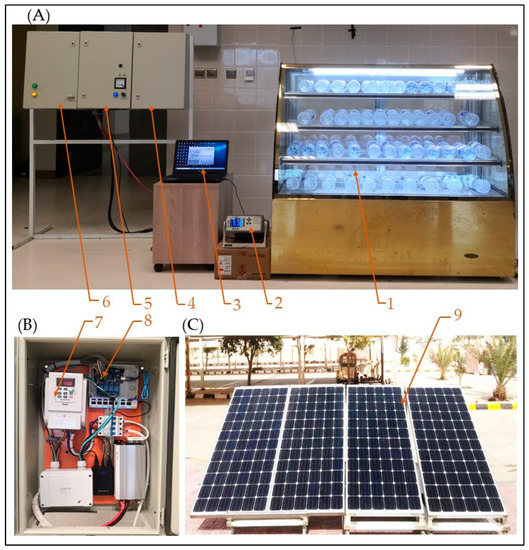
Figure 1.
Different configurations of the experimental setup. (A) Front view of the display refrigerator and control panels, (B) the operation control panel, (C) the solar PV array. (1) The front side of the display refrigerator, (2) the multichannel temperature meter, (3) the PC for data monitoring, (4) the sensor-based frequency control panel, (5) the electrical switches panel, (6) the PV control panel, (7) variable frequency drive (VFD), (8) controller boards (Arduino Mega and relays), and (9) PV array.
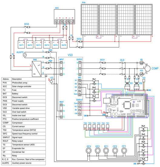
Figure 2.
The block diagram of the solar-powered display refrigerator.
2.1.1. Refrigerator Description
A single-door display refrigerator with a total effective capacity of 0.580 m3 and rated power of 550 W was used in the present study. The main body of this refrigerator was made of tempered vacuum double glass and stainless steel, as shown in Figure 1A. The refrigerator components and their specifications are as follows:
- Cooling cabinet: The dimensions of the refrigerator cooling cabinet were 1.50 m length × 0.70 m width from bottom × 0.19 m width from top × 1.37 m height, 4 shelves, the main body was made from tempered vacuum double glass 0.02 m thick (front, back, and side walls were made from tempered vacuum insulated glass 0.02 m thick), overall heat transfer coefficient is 0.7 W/m2 K. The top and bottom of the cabinet were insulated with 3 cm foam.
- Compressor: The model of the refrigerator compressor was QB91C24GAX0, Panasonic Industrial Kuala Lumpur, Malaysia, with motor type RSIR (Resistance Start Induction Run), one-phase AC 230 V/60 Hz, volumetric capacity 9.07 cm3, oil charge cooling 250 cm3, 710 g refrigerant R134a. This compressor was controlled by the control panel shown in Figure 1B.
- Evaporator: The evaporator tubes were made from copper with a 0.01 m diameter, 0.001 m thickness, and 18.40 m tube length. The maximum suction pressure in the evaporator was 34.5 Pa.
- Evaporator fans: The evaporator was cooled using 3 AC fans 220 V. The dimensions of the fan were 0.04 × 0.12 × 0.12 m with 0.115 m diameter, and the rated power was 20 W.
- Condenser: The condenser was made from a steel tube of 0.01 m diameter, 0.001 m thickness, and 18 m length with steel wire on the tube.
- Condenser fans: The condenser was cooled using 2 AC fans, 220 V. The diameter of each one was 0.25 m, and the rated power was 30 W.
- Lighting unit: The refrigerator was lit using two light-emitting diode strips (LED-Strips) 220 V with 1 m length and rated power 20 W for each.
- Capillary tube: The capillary tube was made from copper with a 3.49 m length, 2.5 mm outer diameter, and 1.0 mm inner diameter.
- Drier cum filter: The diameter of the drier cum filter was 0.04 m and 0.10 m in length.
- Defrost unit: The accumulated frost on the evaporator coils decreases the conduction of the evaporator’s cooling capacity, affecting the cooling efficiency and increasing electrical energy consumption. Therefore, an electric heating coil (220 V, 100 W) was utilized for the defrosting. This heater was clamped directly to the evaporator coil and controlled by a temperature sensor-based defrosting controller.
Table 1 shows the power rating and daily energy consumption for different components of the display refrigerator, such as compressors, evaporator fans (Evap. Fan), condenser fans (Cond. Fan), and lights. In this study, all load components were added together to calculate the total load. In reality, the probability of all maximum loads does not occur simultaneously, but the components were selected on this basis (all max. loads occur at the same time) to ensure that the refrigeration system will not fail.

Table 1.
The power and daily energy consumption of the display refrigerator components.
2.1.2. PV System
The PV system consists of PV modules, batteries, a solar charge controller, and AC/DC inverter. The PV system was installed at King Faisal University, KSA (Latitude: 25°18′ N, Longitude: 49°29′ E, elevation about 179 m above sea level). The sizing details of the PV system are given as follows:
- PV modules: Four PV modules (AS-6P-330 W) were used based on the rated power of the used display refrigerator (Figure 1C). Every 2 PV modules were connected in series, forming 1 string of 91.8 V and 8.85 A. The outputs of the 2 strings were connected in parallel, forming output of 91.8V and 17.7 A. The PV array was inclined 30° toward the south to maximize the insolation on the PV modules. The specifications of PV modules are given in Table 2. To operate the display refrigerator during the night or at not enough insolation, 6 batteries of 12 V and 200 Ah were connected in series and parallel, forming 1 string of 24 V, and used for energy storage, as shown in Figure 2.
Table 2. Different specifications of PV module.
- Charge controller specifications: The following charge controller (PC16-4015 A) was used to charge and protect the batteries. The nominal voltage of the battery output was 12/24 VDC, the open-circuit voltage of PV was 145 VDC at 24 V, the maximum input PV power was 1200 W at 24 V, and the low-voltage protection point was 10.0 VDC/20.0 VDC. As a result, the peak conversion efficiency was 98%.
- Batteries: Due to the discontinuity of solar radiation, the battery bank should be designed with enough capacity to operate the load during the night and at cloudy times. Therefore, this study used six deep-cycle batteries (Lead-Acid Batteries, model: FM250-12, Hefei Greensun Solar Energy Tech Co., Ltd., Hefei, China) with a capacity of 200 Ah and a voltage difference of 12 V, where every 2 batteries were connected in series. The outlets of the 3 groups were connected in parallel so that the final outlet string was 24 V, which is connected to the input of the inverter. The charge and discharge efficiency of the batteries was about 0.8. The required energy storage capacity (Esc) can be estimated by knowing the energy consumption per day and the number of autonomy days (days without charging the battery with a PV system, i.e., without sunshine). Based on the calculations of the electrical loads and the capacity produced by the solar panels, the solar battery system was used to store the electrical energy produced by the solar panels during the sunshine and to operate the display refrigerator during the absence of the sun. During the daytime, the energy produced by the solar panels is used to operate the electrical loads, and the excess solar energy is stored in batteries until needed.
- Solar inverter: MKS-3000, Sunpal Power Co., Ltd., Hefei, China, was used to convert the DC into an AC required to operate the refrigerator. The rated power of this inverter was 3000 VA/2400 W. The DC Input was 24 VDC, 100 AT, the AC output was 230 VAC, 60 Hz, 13 A, and the maximum solar voltage was 145 VDC.
2.1.3. Control System
The present study implemented and investigated two different operating control modes for the solar-powered display refrigerator (SPDR). The first was the traditional control system using a digital temperature controller (model 230 V, XR06CX, Dixell, Pieve d’Alpago, Italy) with fixed compressor speed (FCS) at 230 V/60 Hz. The second mode was the ANN-based control system (ANN-BCS) for controlling variable compressor speed (VCS) and fan operation of the SPDR. The block diagram of the ANN-BCS and electrical circuit of the PV system is given in Figure 2. The control system combined with the solar PV system consisted of a PV array, charge controller, batteries, power supply, variable speed drive system, and control panel. Firstly, the traditional control system (TCS) was used to control the solar-powered display refrigerator using a fixed speed of 60 Hz. Secondly, a developed ANN-BCS with VCS was used for the operation. Finally, the performance of the SPDR was experimentally verified before and after the modification.
The ANN-BCS consisted of several components, i.e., sensors, controller, variable frequency drive, relays, switches, and laptop, as shown in Figure 2. These components were efficiently connected and seamlessly worked to realize the controlling ANN-BCS objectives. The temperature sensors (LM35, Focus Sensing and Control Technology Co., Ltd., Hefei, China) were used for temperature data collection of the SPDR and the ambient temperature surrounding the refrigerator. The temperature and relative humidity (RH) sensor (Model: DHT22, Guangzhou ASAIR Electronic Co., Ltd., Huangpu District, Guangzhou, China) was used to collect data on outside air temperature and RH. The calibrated light intensity sensor module (FUT3101, Ke Zhi You Technology Co., Ltd., Shenzhen, China) was used to collect data on solar irradiance. The current intensity sensors (Load CellX03 with HX711 amplifier, Shenzhen Ke Zhi You Technology Co., Ltd., Shenzhen, Guangdong, China) were calibrated by the second author of the current study [12,29,30]. The main microcontroller was an Arduino Mega board (Microchip ATmega328P, Microchip Technology IncW Chandler Blvd, Chandler, AZ, USA) used to receive and process data and send the control signals to the variable speed drives and the refrigerator devices relays.
The operation and speed of the refrigerator compressor were controlled by a variable speed driver (VFD) with a V/f control transducer (model XSY-AT2, 2.2 kW Jiangsu Changrong Electrical Appliance Co., Ltd., Nanjing, China). The input voltage of the VFD was single phase 220 V, the output voltage was a single phase 220 V, the output current was 10 A, and the output frequency ranged from 0 to 400 Hz. The output VFD frequency can drive a single-phase motor speed. The output frequency of this VFD was controlled by the Arduino, where the Arduino panel sends a signal at the VFD input to change the frequency, as shown in Figure 2.
2.2. Artificial Neural Network Model
In this study, the most common ANN algorithm in machine learning (ML) was trained, evaluated, and deployed in Arduino Mega. The ANN model inputs were the target cooling temperature (Ttar), the internal temperature of the refrigerator (Tref), ambient temperature surrounding the refrigerator (Tamb), solar irradiance at solar panels (SIr), the difference between the internal refrigerator temperature and the target temperature ∆t, and the difference between the ambient temperature and the target temperature ∆T. The output of the ANN model is the equivalent signal to the target frequency and required power. Here is a brief background on the ANN model.
The ANN model is a set of algorithms that simulate the brain’s functioning. The backpropagation algorithm, also known as a multilayered perceptron, is the most common algorism of the artificial ANN. The backpropagation network has neurons arranged in several layers. Generally, the artificial ANN architecture has a three-layered network, as shown in Figure 3. The artificial ANN architecture has one input layer, a hidden layer, and an output layer. The dataset determines the number of input (equals the number of independent variables) and output nodes (response variable), and the number of hidden nodes is more flexible based on the model accuracy. The development of the ANN models is accomplished in the training and testing phases. In the training propagation phase, each node in the hidden and output layers computes a weighted sum of its inputs. After each node’s input weight, the output through the activate function is calculated. The neuron’s output in the artificial ANN generally uses the sigmoidal activate function (Equation (1)).
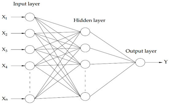
Figure 3.
A simple neural network architecture has three layers: input, hidden, and output. X1, X2, X3, X4, and Xn are the input, and Y is the outcome.
In Figure 3, each input Xi in the input layer is multiplied by its connection weight Wij between each neuron i in the input layer to the neuron j of the hidden layer and obtains its products. Bias Bj is summed formally as net input Ij (Equation (2)) and then passed to the hidden layer by a nonlinear sigmoid activation function (Equation (3)) to produce the output Y as in Equation (4).
2.3. Layout of the Developed Control System
In the current study, two developed control methods were used to control the modified SPDR as follows:
- Multi-speed frequency: The multi-speed frequency-based control method was used to control the SPDR compressor at different frequency speeds, i.e., 40, 45, 50, 55, and 60 Hz, according to the digital signal on speed input frequency control (SIFC) pins of the VSD. Table 3 shows the digital input signals conditions for the multi-speed frequency control method. In the code of this method, the Arduino sends digital low/high signals (low = 0 V and high = 5 V) to the speed input frequency control (SIFC) pins of VSD, as shown in Figure 2. This method was used to create the training dataset to train the ANN model and validate its performance and then deployed in the Arduino to be used in the SPDR control.
Table 3. The digital input signals conditions for the multi-speed frequency control method.
- Variable speed frequency: The variable speed frequency-based control method was used to control the SPDR compressor with variable frequency speeds from 40 to 60 Hz. The code in this method depends on the implemented ANN model and deploying it in Arduino. In this code, the Arduino sends a variable analog signal from 0 to 5 V to the signal input (SINPUT) pin of VSD, as shown in Figure 2. The Arduino output analog signal depends on the target cooling temperature (Ttar), the internal temperature of the refrigerator (Tref), ambient temperature surrounding the refrigerator (Tamb), solar irradiance at solar panels (SIr), the difference between the internal refrigerator temperature and the target temperature ∆t, and the difference between the ambient temperature and the target temperature ∆T.
2.4. The Assumptions and Experimental Operation
The assumptions and experimental operation in this study are as follows:
- Starting to steady processes.
- Pressure drop due to friction in the pipe was considered negligent.
- Comparison between fixed speed compressor (3600 rpm at 230 V/60 Hz) and variable speed using a variable frequency drive (VFD) from 40 to 60 Hz with a V/Hz ratio of 3.83 according to the synchronous speed equation:where N is the compressor motor speed (RPM), f is the input voltage frequency, and P is the number of motor poles (P = 2 in the current study).
- The product was water in well-closed bottles with a total weight of 100 kg. It starts to be cooled from the ambient temperature surrounding the refrigerator for all experiments according to the tested temperature.
2.5. Measurements
The following instruments and methodology were used for the evaluation of the solar PV-powered refrigeration system.
2.5.1. Metrological Data
The metrological data of the experimental site was collected from a weather station at King Faisal University training and research station. Measurements at different setpoints and ambient temperatures in the refrigeration system were conducted using a K-type thermocouple with a multichannel temperature meter (AT4508, Changzhou Applent Instruments Ltd., Changzhou, Jiangsu, China). A pyranometer (Hukseflux-Thermal sensors type LP02, Hiflux Limited, Green Lane, Hounslow TW4 6ER, UK) with a sensitivity of 19.63 μV/Wm2 and reader LI-19 was used to measure insolation on the surface of the PV panel.
2.5.2. PV Sizing
A PV system consists of different units, such as PV modules, solar charge controllers, batteries, inverters, and cables. The PV modules were connected in series and parallel to meet the electric load requirements. The number of PV modules connected in series () and parallel (NPV𝑝) depends on the solar charge controller’s maximum input voltage (Vch.max), maximum input current (Ich.max), the open-circuit voltage (Voc) and short-circuit current (𝐼𝑠𝑐) of the used PV module. The 𝑁PV𝑠 and 𝑁PV𝑝 were calculated as follows:
where Voc is the open-circuit voltage of the PV module (V), and ISC is the short-circuit voltage of the PV module (A). The safety factor of 1.2 and 1.25, respectively, as the limits of Vch.max and Ich.max should never be surpassed [31].
The number of solar charge controllers, N𝑐ℎ.controller, depends on the total number of PV modules NPV, NPV𝑠, and NPV𝑝 within one PV power unit and was calculated as follows:
The PV system nominal power (PPV.𝑛𝑜𝑚) was calculated as follows:
where Pmod.nom is the nominal power of one PV module.
To calculate the hourly PV output power (Pm𝑢𝑛𝑖𝑡), (W) per PV power unit at hour t (1 ≤ t ≤ 8760), the hourly ambient temperature 𝑇𝑎mb (𝑡) (°C), and the hourly global insolation on PV module Ins(t, ) (W/m2) installed at (°) tilt angle were used:
where Tc(t) is the hourly cell temperature (°C), NOCT is the nominal operating cell temperature (°C), Voc (t)the hourly open-circuit voltage (V), 𝐾𝑉 is the open-circuit voltage temperature coefficient (V/°C), Isc (T, 𝐼𝑠𝑐(𝑡, 𝛽) is the hourly short-circuit current (A), KI is the short-circuit current temperature coefficient (A/°C), and FF is the fill factor [32].
The actual hourly PV power output from the solar charge controller depends on its efficiency as follows:
where is the charge controller efficiency (%).
The total PV power produced by the PV system was calculated as follows:
2.5.3. PV Panel Efficiency
The PV panel efficiency () was computed as follows [9]:
where Pmax is the maximum power generated by the PV array (W), Pin is the total input power (irradiation) (W), Imax is the maximum current generated from the PV array (A), Vmax is the maximum voltage of PV array (V), InsPV is the irradiation on the PV array surface (W/m2), and APV is the area of the PV array (m2).
2.5.4. Power and Electrical Energy
The AC voltage, current, frequency, and power factor of the SPDR were measured using a digital power clamp meter UT131 (UNI-T, Uni-Trend Technology Co., Ltd. Dongguan, Guangdong, China). The following formula was used to estimate the electrical power and energy consumption:
where P is the refrigerator power for the single phase, is the voltage (line to neutral), I is the current intensity, PF is the power factor (), E is the energy consumption, and T is the operating time.
The energy generated by the PV system was measured using a 150 A digital Watt meter (WATTMETER—150, 0–6554 Wh, Shenzhen Resky Electronics Co., Ltd., Shenzhen, China).
2.5.5. Cooling Load
The cooling loads were estimated as follows [33,34]:
- Walls and roof: The sensible heat gain through the walls, floor, and roof of the refrigerator was separately calculated as a steady state using the following formula:where Q1 is the heat gain (kWh/d), A is the outside area of the section (m2), U is the coefficient of heat transfer (W/m2 K), Tamb is the outside air temperature (K), and Tref is the temperature inside the refrigeration (K).
- Product cooling load: The following formula was used to calculate the cooling load of the product from the initial temperature to the refrigerator’s target temperature:where Q2 is the product cooling load (kWh/d), CP is the specific heat capacity of the product (KJ/kg K), m is the mass of the products (kg), Tint is the initial input temperature of the products (K), Tref is the temperature inside the refrigeration (K).
- Cooling load from product inhaler: The cooling load from the inhaler product was considered negligent because the product was water in well-closed bottles.
- Internal heat load: The cooling load from illumination (heat generated by lighting) was calculated using the following formula:where Q3 is the heat load generated by the lighting (kWh/day), Nl is the number of lamps in the refrigerator, T is the daily working time, and P is the power rating of the lamps.
- Produced heat by fans: The produced heat by fans was calculated using the following formula:where Q4 is the heat load generated by the fans (kWh/day), Nf is the number of fans in the refrigerator, T is the daily working time, and P is the nominal power of the fan motors.
- Produced heat by defrost: The produced heat by defrost was calculated using the following formula:where Q5 is the heat load generated by the defrost (kWh/day), Dc is the number of times the defrost cycle occurs per day, T is the defrost working time, P is the power rating of the heater (KW), and η is the percentage of heat transferred to the environment (η = 0.35).
The total cooling load (Q, kWh/d) was determined by collecting all the determined cooling load values. To consider the errors or non-considered parameters, a safety factor of 20% was also applied in the calculation. The following formula was used to calculate the total cooling load:
2.5.6. Coefficient of Performance
The coefficient of performance (COP) is one of the common methods to evaluate refrigerators’ efficiency [35]. The efficiency of a refrigerator is the ratio of energy output to energy input. The energy output is the desired energy quantity to achieve the cooling, while the energy input is work performed by the refrigerator. The working substance extracts some heat Qc from the cold zone at temperature Tc, and the external work W is performed on it while heat Qh is removed to the hot environment at temperature (Th), as shown in Figure 4.
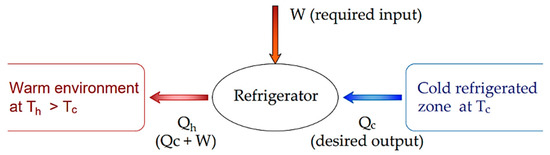
Figure 4.
Schematic representation of refrigerator thermodynamics.
The heat the refrigerator receives (Qc), and the work applied (W) are rejected to the warm environment at a temperature Th. Based on the first law of thermodynamics, the amount of heat rejected Qh equals Qc plus W. The heat removed from the refrigerated zone divided by the energy input needed to do so is known as the coefficient of performance (COP) as follows:
Considering the Qh = Qc + W, the COP of the refrigerator was expressed in terms of the heat as follows:
where COP is the coefficient of performance of a refrigerator, Qc is the removed heat from the refrigerated zone, W is the required work, and Qh is the removed heat to the warm environment.
The best possible COP of a refrigerator that operates with Carnot efficiency is expressed as follows [35]:
where COPmax is the maximum coefficient of performance of a refrigerator, Qlow and Qhigh are the high and low amount of heat (kJ), and Tlow and Tmax are the low and high temperature (K).
2.6. Instrument Uncertainty
Uncertainties correlated with the instruments used for measurements are presented in Table 4. Uncertainty about instruments is associated with systematic errors and can be obtained from the instrument’s calibration report or data book. Also, the standard uncertainty “U” for the measuring instruments can be calculated by the following equation [36,37]:
where ac = accuracy of the instrument.
Table 4.
Uncertainty of different measuring instruments.
2.7. Statistical Analysis, Software Platforms, ANNs Evaluation
The statistical analysis was performed using one-way analysis of variance (ANOVA) at p ˂ 0.05 using Statistical Analysis Software, IBM SPSS version 26 (SPSS Inc., Chicago, IL, USA). Design Expert software (DX Version 13, Stat-Ease, Inc., Minneapolis, MN, USA) was used to plot the effect of the variables on the studied parameters. The ANN model was developed and deployed using licensed ANNHUB software (ANNHUB Version 1.6.0.0, ANSCENTER Co., Sydney, Australia).
The coefficient of determination (R2) and the root mean square error (RMSE) meters were used to evaluate the performance of the ANN mode by using the following formulas:
where Oj is the observed value, Pj is the predicted value of data j, and n is the number of values.
3. Results and Discussion
3.1. Meteorological Data
Figure 5 shows the different weather parameters, including the solar radiation, temperature, and relative humidity of the experimental site. The daily average solar radiation varied from 164.41 W/m2 in February to 322.58 W/m2 in June, as shown in Figure 5A. The maximum solar radiation ranged from 745 to 1048 W/m2 during Dec and April. At the same time, the average maximum daily solar radiation varied from 642.6 to 983.8 W/m2 during Jan and June, respectively.
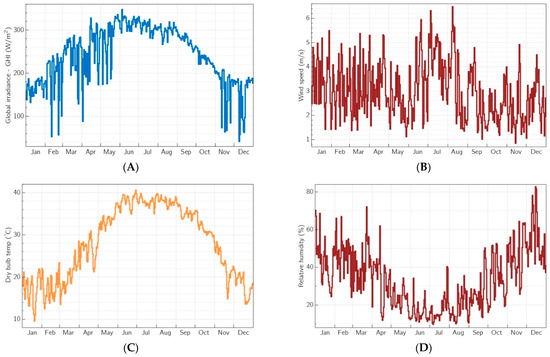
Figure 5.
Average daily irradiance (A), wind speed (B), temperature (C), and relative humidity of the experimental site (D).
The daily average wind speed ranged from 2.03 to 4.1 m/s during September and June, respectively, as shown in Figure 5B. The maximum daily wind speed varied from 0.82 m/s to 6.9 m/s, respectively. The average daily max wind speed changed from 3.6 m/s in Sept to 6.9 m/s in June. The daily average temperature ranged from 14.7 °C during February to 39.31 °C during July, as shown in Figure 5C, while the average daily max temperature varied from 47.7 °C in July to 20.9 °C in February. The daily average relative humidity ranged from 14% during June to 48.36% during February, as shown in Figure 5D, while the average daily max temperature ranged from 24.9% during June to 72.47% during February. In the current study, the wind speed did not negatively impact the PV system. However, it is still essential to consider the potential effects of wind when designing and installing a PV system to ensure its long-term efficiency and reliability. The impact of wind speed on the performance and design of a solar PV system should be considered in PV module installation. Wind speed affects the temperature and cooling of PV panels, affecting their efficiency and power output. High wind speeds can also cause mechanical stress and damage to the system, making it essential to design the system to withstand such loads. The location and orientation of the PV panels may also need to be optimized based on local wind conditions to ensure the long-term efficiency and reliability of the system.
The presented results indicated that the highest irradiation and temperature were recorded during the summer while the lowest levels were recorded during the winter months which affect the performance of the display refrigerator. The highest temperature occurred at the highest irradiation, where the PV-generated energy was enough to overcome the running time of the display refrigerator.
3.2. PV System Performance
The performance of the PV array was evaluated outdoors. As shown in Figure 6, the ambient conditions affected the PV array performance. The results indicated that the irradiation on the PV array surface varied from 385 to 1025 W/m2 with a daily average of 846.03 W/m2 (Figure 6A). The highest irradiation occurred around noon. The wind speed values ranged from 1.4 to 3.2 m/s, with a daily average of 2.26 m/s. The highest wind speed value occurred in the morning and occasionally varied for the rest of the day. The ambient temperature ranged from 29.5 to 44.8 °C with a daily average of 39.5 °C while the solar PV array temperature varied from 33.9 to 55.2 °C with a daily average of 47.4 °C (Figure 6B). It can be noticed that the solar radiation and ambient temperature affected the PV array performance. The PV panel temperature has a direct proportionality with the ambient temperature. The PV panel temperature increased by increasing the ambient temperature. The daily average PV panel temperature was higher than the daily average surrounding temperature by 7.91 °C.
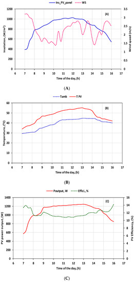
Figure 6.
Effect of ambient conditions on PV modules performance. (A) Solar radiation and wind speed, (B) PV panel and ambient temperature, (C) PV power output and PV panel efficiency.
Figure 6C shows the PV power output and conversion efficiency over the daytime. The panel power output varied from 571.3 to 1247.1 W at 7 am and 1 pm, respectively, while the daily average was 1.098 kW. The higher solar radiation led to a higher power output from the PV around noon. Increasing the PV panel temperature caused a reduction in the open-circuit voltage and an increase in the short-circuit current. The PV panel conversion efficiency varied from 10.82 to 14.2% at 11:30 A.M. and 4 P.M., respectively, and the daily average was 11.47%. The higher efficiency was recorded during the early and late hours of the day when the PV array had a lower temperature. At the same time, the lower temperature was recorded around noon due to the higher temperature of the PV panel. Also, the surrounding wind speed affected the PV panel temperature and its conversion efficiency. These results are in agreement with [29,38].
3.3. Training Dataset
The optimum SPDR power requirement was achieved in the current study by optimizing the applied frequency. This optimization aims to achieve optimum energy consumption under different variable conditions to reduce the required PV size. Therefore, the desirability function approach was used to analyze the experiments because the multi-variables and responses need to be optimized simultaneously [22].
The optimum frequencies that were used to train the ANN were determined by conducting preliminary experiments, including the implementation and optimization criterion using Design Expert software to minimize the electrical power requirement by optimizing the applied frequency at 40, 45, 50, 55, and 60Hz, under a T_Tar equal to 1, 2, 3, 4, and 5 °C, and the T_Ref in a range from 6 to 30 °C, T_Amb in a range from 16 to 40 °C, S_Irr in a range from 0 to 500 W/m², ∆t in a range from 5 to 25 °C, and ∆T in a range from 15 to 35 °C.
The energy requirement must be as small as possible to decrease the PV cost while maintaining the refrigeration target. Therefore, we prepared the training dataset after conducting the experiments at optimum frequency and electrical power requirements. The ANN training dataset included the optimum frequency based on the target cooling temperature (T_Tar), the internal temperature of the refrigerator (T_Ref), the ambient temperature surrounding the refrigerator (T_Amb), the solar irradiance at solar panels (S_Irr), the difference between the internal refrigerator temperature and the target temperature (∆t), and the difference between the ambient temperature and the target temperature (∆T).
Figure 7 shows the average frequency values under the studied factors of A: T_Tar, B: T_Amb, C: T_Ref, D: ∆T, E: ∆t, and S_Irr. Figure 8 shows the average required power for the SPDR at the optimum frequency. The result indicated that the measured values of the frequency were near what was determined to satisfy the optimization criteria. Based on the optimum value of the frequency, the training dataset was created to develop the ANN prediction models.
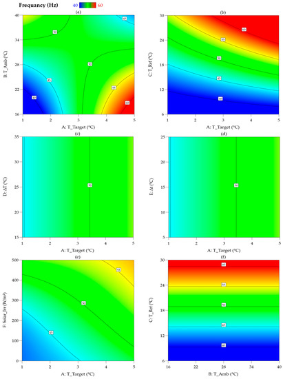
Figure 7.
The average values of the frequency under the studied factors of A: T_Tar and B: T_Amb (a), A: T_Tar and C: T_Ref (b), A: T_Tar and D: ∆T (c), A: T_Tar and E: ∆t (d), A: T_Tar and S_Irr (e), and B: T_Amb and C: T_Ref (f).
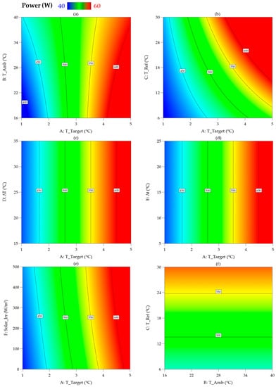
Figure 8.
The average values of the required power for the SPDR under the studied factors of A: T_Tar and B: T_Amb (a), A: T_Tar and C: T_Ref (b), A: T_Tar and D: ∆T (c), A: T_Tar and E: ∆t (d), A: T_Tar and S_Irr (e), and B: T_Amb and C: T_Ref (f).
3.4. Evaluation of the ANNs Model
The ANN technique in the ANNHUB software was used to determine the optimal prediction model to predict the optimum frequency and the required power for the SPDR based on the training dataset. In the current study, we set the platform of ANNHUB to design an ANN for prediction. Therefore, it automatically selects the Levenberg–Marquardt algorithm. In its form for the ANN, the Levenberg–Marquardt algorithm considers the iterative optimization of the weights in a compound estimation of the outputs in the training phase, not only as a function of the inputs but also of the state variables series [39]. After configuring the ANN in the platform ANNHUB, the ANN was trained, as shown in Figure 9. The best validation performance was 0.00091 at epoch 10 of the training attempts.
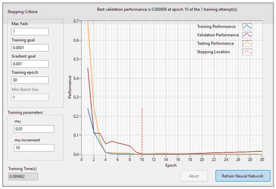
Figure 9.
Train the artificial neural networks in ANNHUB.
In the current study, stopping criteria were used in the ANN training phase to end or stop the training process based on different parameters, i.e., the training goals, training epoch, and gradient goal. For example, the training process will stop if the cost function value is less than 0.0001 or the gradient value is less than 0.01. During the training phase, the ANN uses all the training data inputs to estimate the model outputs, which are then compared to the training data targets to optimize the cost function. The training epoch value is also used as a stopping criterion, halting the training process when it exceeds 30.
Figure 9 displays the training process for developing the ANN model based on the training datasets. The hidden layer was one with eight neurons excluding the bias node, the input layer contains six neurons for the independent variables, i.e., Ttar, Tref, Tamb, SIr, ∆t, and ∆T, and the output is the equivalent signal to the target frequency and the required power.
Table 5 provides detailed information on the developed ANN for frequency and power prediction. The input layer consists of six independent variables standardized to have a mean of zero and a standard deviation of one. In contrast, the output layer has a single dependent variable, frequency, which is also standardized. The neural network was trained using the Levenberg–Marquardt optimization algorithm, with 75% of the data used for training and 25% for testing.
Table 5.
ANN configuration for frequency and power prediction using the Levenberg–Marquardt training engine.
The backpropagation optimized the ANN performance for frequency and power prediction by minimizing the mean squared error cost function during training. The optimization process using backpropagation involves iteratively adjusting the network’s weights and biases based on the gradient of the error. First, the algorithm propagates the error backward from the output layer to the input layer, computing the gradients for each layer along the way. The gradients are then used to update the weights and biases in the opposite direction of the gradient, to minimize the error or cost function. This process continues until the error is minimized to an acceptable level or until a specified number of iterations have been reached. Therefore, the ANN predicted the frequency and power output as accurately as possible while minimizing the mean squared difference between the predicted and actual frequency values. The backpropagation algorithm is a powerful tool for optimizing the neural network performance and can be used in various applications [40].
Figure 10 displays the scatter plots of the target values of the frequency and required power for the SPDR operation versus the predicted values by the ANN models in the evaluation phase based on the training dataset. Again, the selected network structure of the ANN model exhibited high accuracy.
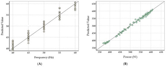
Figure 10.
Regression curves to evaluate the trained ANN model for the optimal frequency (A) and required power (B) for SPDR operation.
The performance evaluation of the ANN models for the frequency and power of the SPDR based on the R2 and RMSE values is shown in Table 6. The high R2 and low values of the RMSE indicate that the ANN model presents good possibilities to deploy and use for the Arduino control code based on the input variables. Furthermore, based on the R2 and RMSE values in Table 5, it is indicated that the ANN modeling algorithm was efficient in deploying for controlling the output frequency. Based on these findings, the ANN model was deployed and used for VFD control.
Table 6.
R2, RMSE, and fit line equations for the developed ANNs models in the evaluation phase.
3.5. Evaluation of Refrigerator Performance
The evaluation results of the developed ANN model showed the possibility of predicting the frequency and power required for the SPDR based on input variables with high accuracy. Therefore, the developed ANN model was deployed on an Arduino board to control the solar-powered display refrigerator (SPDR) operation. To evaluate the performance of the SPDR under the ANN-based control system, the SPDR was operated under 3 targeted temperatures of 1, 3, and 5 °C. The SPDR was operated under variable frequencies from 40 to 60 Hz. The performance of the SPDR was compared with its performance under the traditional control system at a fixed frequency of 60 Hz. The following is the evaluation of the different parameters of the SPDR under two control systems.
3.5.1. Frequency
Figure 11 shows the average daily frequency of the SPDR with a modified ANN-based control system (MR) (Figure 11A) and the SPDR with a traditional control system (TR) (Figure 11B). Generally, there was a significant difference (p < 0.05) in the average daily frequency between the MR and TR. The following is the influence of the target temperatures under different ambient temperatures on the average daily frequency of the MR and TR:
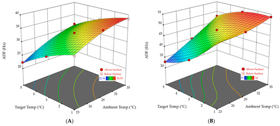
Figure 11.
Average daily frequency (ADF) of the solar-powered refrigerator (SPDR) with a modified ANN-based control system (A) and the SPDR with a traditional control system (B).
- Target product temperature (1 °C): At an average ambient temperature of 23 °C, the average daily frequency (ADF) was 31.92 ± 21.43 Hz and 49.96 ± 22.41 Hz for the MR and TR, respectively. At an average ambient temperature of 29 °C, the ADF was 37.31 ± 22.45 Hz and 50.58 ± 21.83 Hz for the MR and TR, respectively. While at an average ambient temperature of 35 °C, the ADF was 38.53 ± 22.69 Hz and 53.71 ± 18.39 Hz for the MR and TR, respectively. The ADF for the TR was higher than the MR, with 18.08 Hz, 13.27 Hz, and 15.18 Hz at ambient temperatures of 23, 29, and 35 °C, respectively.
- Target product temperature (3 °C): At an average ambient temperature of 23 °C, the average daily frequency (ADF) was 28.17 ± 21.5 Hz and 38.38 ± 28.82 Hz for the MR and TR, respectively. At an average ambient temperature of 29 °C, the ADF was 33.35 ± 20.4 Hz and 47.71 ± 24.22 Hz for the MR and TR, respectively. While at an average ambient temperature of 35 °C, the ADF was 35.69 ± 20.9 Hz and 52.92 ± 19.37 for the MR and TR, respectively. The ADF for the TR was higher than the MR, with 10.21 Hz, 14.36 Hz, and 17.23 Hz at ambient temperatures of 23, 29, and 35 °C, respectively.
- Target product temperature (5 °C): At an average ambient temperature of 23 °C, the average daily frequency (ADF) was 22.34 ± 21.95 Hz and 32.88 ± 29.87 Hz for the MR and TR, respectively. At an average ambient temperature of 29 °C, the ADF was 27.05 ± 22.35 Hz and 40 ± 28.29 Hz for the MR and TR, respectively. While at an average ambient temperature of 35 °C, the ADF was 31.25 ± 21.03 Hz and 47.83 ± 24.13 Hz for the MR and TR, respectively. The ADF for the TR was higher than the MR, with 10.54 Hz, 12.95 Hz, and 16.58 Hz at ambient temperatures of 23, 29, and 35 °C, respectively.
Generally, increasing the ambient temperature led to an increase in the running time of the refrigerator and hence an increase in the ADF.
3.5.2. Power Consumption
The obtained results of the voltage revealed that at a product temperature of 1 °C and an average daily temperature of 23 °C, the refrigeration system voltage was about 122.35 ± 82.08 V and 183.18 ± 82.15 V for the MR and TR, respectively. At a product temperature of 1 °C and an average daily temperature of 29 °C, the refrigeration system voltage was about 142.97 ± 86 V and 185.47 ± 80.05 V for the MR and TR, respectively. While at a product temperature of 1 °C and an average daily temperature of 35 °C, the refrigeration system voltage was about 147.66 ± 86.94 V and 196.93 ± 67.43 V for the MR and TR, respectively.
On the other hand, when the product temperature was 5 °C and the average daily temperature was 23 °C, the refrigeration system voltage was about 85.65 ± 84.07 V and 120.54 ± 109.53 V for the MR and TR, respectively. At a product temperature of 5 °C and the average daily temperature of 29 °C, the refrigeration system voltage was about 103.68 ± 85.63 V and 146.67 ± 103.75 V for the MR and TR, respectively. While at a product temperature of 5 °C and the average daily temperature of 35 °C, the refrigeration system voltage was about 119.76 ± 80.56 V and 175.39 ± 88.49 V for the MR and TR, respectively. It should be noted that there is a direct relationship between the frequency and voltage, i.e., increasing the frequency causes an increasing voltage and vice versa.
The obtained results of the current intensity revealed that at a product temperature of 1 °C and an average daily temperature of 23 °C, the refrigeration system current was about 1.86 ± 1.19 A and 1.94 ± 1.27 A for the MR and TR, respectively. At a product temperature of 1 °C and an average daily temperature of 29 °C, the refrigeration system current was about 1.86 ± 1.19 A and 2.26 ± 1 A for the MR and TR, respectively. While at a product temperature of 1 °C and an average daily temperature of 35 °C, the refrigeration system current was about 2.02 ± 1.11 A and 2.4 ± 0.85 A for the MR and TR, respectively.
For a 3 °C product temperature and 23 °C average daily temperature, the refrigeration system current was about 1.71 ± 1.25 A +1.76 ± 1.34 A for the MR and TR, respectively. At a 3 °C product temperature and 29 °C average daily temperature, the refrigeration system current was about 1.96 ± 1.14 A and 2.2 ± 1.15 A for the MR and TR, respectively. While at a 3 °C product temperature and 35 °C average daily temperature, the refrigeration system current was about 2.01 ± 1.12 A and 2.35 ± 0.9 A for the MR and TR, respectively.
On the other hand, when the product temperature was 5 °C and the average daily temperature was 23 °C, the refrigeration system voltage was about 1.39 ± 1.31 A and 1.5 ± 1.4 A for the MR and TR, respectively. At a product temperature of 5 °C and the average daily temperature of 29 °C, the refrigeration system voltage was about 1.61 ± 1.28 A and 1.81 ± 1.31 A for the MR and TR, respectively. While at a product temperature of 5 °C and the average daily temperature of 35 °C, the refrigeration system voltage was about 1.87 ± 1.19 A and 2.16 ± 1.12 A for the MR and TR, respectively.
Figure 12 shows the average daily power (ADP) consumption of the solar-powered display refrigerator (SPDR) with a modified ANN-based control system (MR) and the SPDR with a traditional control system (TR) when the average daily temperature was about 29 °C and the product temperature was 3 °C for one day. It is clear from Figure 12 the developed control system operates the refrigeration system very smoothly compared to the traditional one. Also, the power consumption by the TR was higher than the MR.
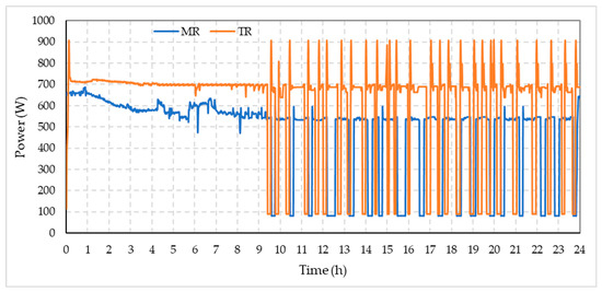
Figure 12.
Average daily power (ADP) consumption of the solar-powered refrigerator (SPDR) with a modified ANN-based control system (MR) and the SPDR with a traditional control system (TR).
Figure 13 shows the average daily power (ADP) consumption of the MR (Figure 13A) and TR (Figure 13B). There was a significant difference (p < 0.05) in the ADP between the MR and TR. The following is the influence of the target temperatures under different ambient temperatures on the ADP of the MR and TR:
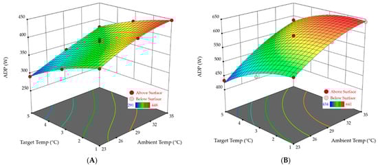
Figure 13.
Average daily power (ADP) consumption of the solar-powered refrigerator (SPDR) with a modified ANN-based control system (A) and the SPDR with a traditional control system (B).
- Target product temperature (1 °C): The ADP consumption of the refrigerators at an average ambient temperature of 23 °C was 382.63 ± 204.5 W and 536.62 ± 285.86 W for the MR and TR, respectively. At an average ambient temperature of 29 °C, the ADP consumption by the refrigeration system was 427.35 ± 224.88 W and 607.53 ± 228.37 W for the MR and TR, respectively. While at the average ambient temperature of 35 °C, the ADP consumption was about 447.61 ± 217.12 W and 641.02 ± 194.25 W for the MR and TR, respectively. The results indicated that the power consumption by the TR was higher than the MR at all times by 153.99 W, 180.18 W, and 193.41 W at an average ambient temperature of 23 °C, 29 °C, and 35 °C, respectively. This revealed that increasing the ambient temperature increased the running time of the refrigerator, which resulted in higher power consumption.
- Target product temperature (3 °C): At an average ambient temperature of 23 °C, the ADP consumption of the refrigerators was about 346.79 ± 206.07 W and 492.52 ± 307.55 W for the MR and TR, respectively. At an average ambient temperature of 29 °C, the ADP consumption by the refrigeration system was 397.03 ± 194.71 W and 593.06 ± 262.77 W for the MR and TR, respectively. While at the average ambient temperature of 35 °C, the ADP consumption was about 419.67 ± 200.34 W and 630.01 ± 205.13 W for the MR and TR, respectively. The results showed that the power consumption by the TR was higher than the MR, with 145.73 W, 196.03 W, and 210.34 W at an average ambient temperature of 23 °C, 29 °C, and 35 °C, respectively.
- Target product temperature (5 °C): The ADP consumption of the refrigerators at an average ambient temperature of 23 °C was 291.24 ± 211.41 W and 433.98 ± 319.4W for the MR and TR, respectively. At an average ambient temperature of 29 °C, the ADP consumption by the refrigeration system was 336.76 ± 214.57 W and 505.95 ± 299.31 W for the MR and TR, respectively. While at the average ambient temperature of 35 °C, the ADP consumption was about 377.1 ± 201.82 W and 584.62 ± 256.62 W for the MR and TR, respectively. The results indicated that the power consumption by the TR was higher than the MR at all times by 142.74 W, 169.19 W, and 207.52 W at an average ambient temperature of 23 °C, 29 °C, and 35 °C, respectively.
This revealed that increasing the ambient temperature increased the running time of the refrigerator, which resulted in higher power consumption.
From the above results, it is obvious that at a 1 °C product temperature, the MR can save power about 28.7%, 29.7%, and 30.2% compared to the TR at the average ambient temperature of 23 °C, 29 °C, and 35 °C, respectively. At a 3 °C product temperature, the MR can save power about 29.6%, 33.1%, and 33.4% compared to the TR at the average ambient temperature of 23 °C, 29 °C, and 35 °C, respectively. While at a 5 °C product temperature, the MR can save power about 32.9%, 33.4%, and 35.5% compared to the TR at the average ambient temperature of 23 °C, 29 °C, and 35 °C, respectively. It is clear that the developed control system performed well compared to the traditional one and is expected to provide the basis for designing and optimizing the PV-powered refrigeration system. The trend of the output results is in agreement with [41].
In a previous study conducted by Hamad et al. [42], it was noted that reducing the compressor speed to 35 Hz and using a 2% vapor injection could extend the compressor’s lifetime by decreasing the ON/OFF cycle of the system by 17.3% compared to a conventional system. However, at 60Hz, the ON/OFF cycle increased by 9.3% and 12% for the 2% and 4% injection ratios, respectively. Furthermore, comparing the experimental and numerical results for the modified system with a vapor injection ratio of 2% and a compressor speed of 35Hz revealed an increase in the COP of approximately 2.57%, a cooling capacity of 5.8%, and compressor power consumption of 5.68%.
3.5.3. Energy Consumption
Figure 14 shows the MR (Figure 14A) and TR (Figure 14B) average daily energy consumption. The following is the influence of the target temperatures under different ambient temperatures on the average daily energy consumption:
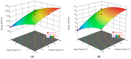
Figure 14.
Average daily energy consumption of the solar-powered refrigerator (SPDR) with a modified ANN-based control system (A) and the SPDR with a traditional control system (B).
- Target product temperature (1 °C): At an average ambient temperature of 23 °C, the average energy consumption of the refrigeration system was about 9.18 ± 1.23 kWh/d and 12.88 ± 2.21 kWh/d for the MR and TR, respectively. At an average ambient temperature of 29 °C, the average energy consumption by the refrigeration system was about 10.26 ± 1.02 kWh/d and 14.58 ± 1.24 kWh/d for the MR and TR, respectively. While at the average ambient temperature of 35 °C, the average energy consumption was about 10.74 ± 1.08 kWh/d and 15.38 ± 1.45 kWh/d for the MR and TR, respectively. The results showed that the average energy consumption of the TR was higher than the MR by 3.7 kWh/d, 4.32 kWh/d, and 4.64 kWh/d at an average ambient temperature of 23 °C, 29 °C, and 35 °C, respectively.
- Target product temperature (3 °C): The average energy consumption of the refrigerators at an average ambient temperature of 23 °C was 8.32 ± 1.01 kWh/d and 11.82 ± 1.23 kWh/d for the MR and TR, respectively. At an average ambient temperature of 29 °C, the average daily energy consumption of the refrigeration system was about 9.53 ± 1.22 kWh/d and 14.23 ± 1.11 kWh/d W for the MR and TR, respectively. While at the average ambient temperature of 35 °C, the ADP consumption was about 10.07 ± 1.22 kWh/d and 15.12 ± 1.21 kWh/d for the MR and TR, respectively. The results indicated that the average energy consumption of the TR was higher than the MR at all times by 3.5 kWh/d, 4.7 kWh/d, and 5.05 kWh/d at an average ambient temperature of 23 °C, 29 °C, and 35 °C, respectively. This revealed that increasing the ambient temperature increased the running time of the refrigerator, which resulted in higher energy consumption per day.
- Target product temperature (5 °C): The average daily energy consumption of the refrigerators at an average ambient temperature of 23 °C was 6.99 ± 1.04 kWh/d and 10.42 ± 1.09 kWh/d for the MR and TR, respectively. At an average ambient temperature of 29 °C, the average daily energy consumption by the refrigeration system was about 8.08 ± 1.08 kWh/d and 12.14 ± 1.12 kWh/d, respectively. While at the average ambient temperature of 35 °C, the average daily energy consumption was about 9.05 ± 1.21 kWh/d and 14.03 ± 1.21 kWh/d for the MR and TR, respectively. The results indicated that the average energy consumption by the TR was higher than the MR at all times by 3.43 kWh/d, 4.06 kWh/d, and 4.98 kWh/d at an average ambient temperature of 23 °C, 29 °C, and 35 °C, respectively. This revealed that increasing the ambient temperature increased the running time of the refrigerator, which resulted in higher power consumption.
Compared to the TR, the results indicated that the MR saves energy about 32.91% at an average ambient temperature of 23 °C, about 33.44% at 29 °C, and 35.5% at 35 °C. Meanwhile, the refrigeration system was operated with a PV system useful for rural or remote areas. The obtained results agree with Chu et al. [43], who investigated the thermal comfort control on a multi-room fan coil unit system using LEE-based fuzzy logic. They mentioned that applying fuzzy logic techniques in the control system can reduce energy consumption by 30% daily. Using solar-powered refrigerators as an alternative to compressor-operated refrigerators has many benefits, such as saving the environment, cost, and health [44]. Selvaraj and Victor [11] noted that renewable energy sources could help meet energy demands sustainably without compromising the environment or future energy needs. A 525.6 kWh energy saving was achieved in the PV-integrated DC system, and even the 10.2-year payback is considered pretty good for a system that operates for 30 years.
3.5.4. Power Consumption of Fans
Figure 15 shows the average daily fan power (ADFP) consumption of the MR (Figure 15A) and TR (Figure 15B). The following is the influence of the target temperatures under different ambient temperatures on the average daily energy consumption:
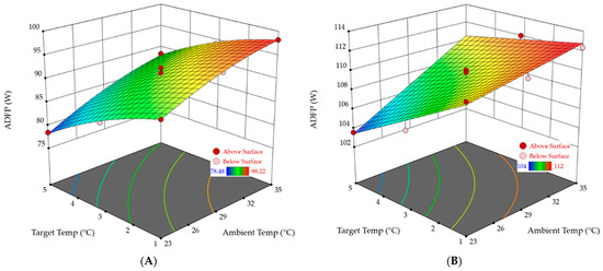
Figure 15.
Average daily fan power (ADFP) consumption of the solar-powered refrigerator (SPDR) with a modified ANN-based control system (A) and the SPDR with a traditional control system (B).
- Target product temperature (1 °C): At an average ambient temperature of 23 °C, the ADFP consumption (of the refrigeration system) was about 78.48 ± 7.94 W and 110.82 ± 9.34 W for the MR and TR, respectively. At an average ambient temperature of 29 °C, the ADFP consumption was about 78.68 ± 7.85 W and 111.08 ± 9.1 W for the MR and TR, respectively. While at the average ambient temperature of 35 °C, the ADFP consumption was about 78.68 ± 7.85 W and 112.38 ± 7.66 W for the MR and TR, respectively.
The results showed that the ADFP consumption of the TR was higher than the MR by 32.34 W, 32.32 W, and 33.7 W at an average ambient temperature of 23 °C, 29 °C, and 35 °C, respectively. It should be noted that the developed system controls the fan operation based on the temperature difference between the evaporator and the cabinet. For example, when the temperature of the evaporator and cabinet are equal, the system stops working, saving energy.
- Target product temperature (3 °C): At an average ambient temperature of 23 °C, the ADFP consumption (of the refrigeration system) was about 78.48 ± 7.94 W and 105.99 ± 12.01 W for the MR and TR, respectively. At an average ambient temperature of 29 °C, the ADFP consumption was about 78.68 ± 7.85 W and 109.88 ± 10.09 W for the MR and TR, respectively. While at the average ambient temperature of 35 °C, the ADFP consumption was about 78.68 ± 7.85 W and 112.05 ± 8.07 W for the MR and TR, respectively.
- Target product temperature (5 °C): The ADFP consumption of the refrigerators at an average ambient temperature of 23 °C was 78.48 ± 7.94 W and 103.57 ± 13.02 W for the MR and TR, respectively. At an average ambient temperature of 29 °C, the ADFP consumption by the refrigeration system was about 78.68 ± 7.85 W and 106.67 ± 11.79 W for the MR and TR, respectively. While at the average ambient temperature of 35 °C, the ADFP consumption was about 78.68 ± 7.85 W and 109.93 ± 10.06 W for the MR and TR, respectively.
The results indicated that the ADFP consumption of the TR was higher than the MR by 27.51 W, 31.2 W, and 33.37 W at an average ambient temperature of 23 °C, 29 °C, and 35 °C, respectively. Meanwhile, the ADFP consumption of the TR was higher than the MR by 25.09 W, 27.99 W, and 31.25 W at an average ambient temperature of 23 °C, 29 °C, and 35 °C, respectively.
This means when the product temperature was 1 °C, the ADFP consumption of the TR was greater than the MR by 29.18%, 29.17%, and 29.99% at an average ambient temperature of 23 °C, 29 °C, and 35 °C, respectively. When the product temperature was 3 °C, the ADFP consumption of the TR was greater than the MR by 25.96%, 28.39%, and 29.78% at an average ambient temperature of 23 °C, 29 °C, and 35 °C, respectively. While the product temperature was 5 °C, the ADFP consumption of the TR was greater than the MR by 24.23%, 26.24%, and 28.43% at an average ambient temperature of 23 °C, 29 °C, and 35 °C, respectively. A data analysis revealed that the TR’s ADFP consumption was significantly greater than the MR at the same tested conditions. The reason for that is the developed system controlling the fan operation based on the temperature difference between the evaporator and the cabinet.
Rajoria et al. [45] investigated the performance variation in a solar PV-powered refrigeration system combined with storage batteries. The authors analyzed the change in the battery voltage concerning the panel size through an experimental investigation using 4 solar PV panels of 35 W, each connected in different series and parallel combinations to obtain 24 V and a current ranging from 3–5 amperes, based on the solar intensity. The used refrigerator with a capacity of 50 L consumed 110 W and required 0.80 amperes AC at 230 V. To obtain the necessary voltage and current, the inverter drew about 7 amperes DC from the battery bank at 24 V. The refrigerator compressor consumed 110 W, requiring a PV panel size of approximately 176 W. However, the compressor consumed about 300 W for the first 50 milliseconds, 130 W for the next 5 s, and gradually reduced to 110 W in 65 s. The authors emphasized that the PV panel size should be sufficient to compensate for the initial load requirement. Our study also observed that the PV system consumes approximately 10% of the energy when comparing the power drawn from the direct current and the actual power consumed by the developed refrigerator. In addition, the current needed to operate at the beginning of the movement of the refrigerator compressor at 60 Hz. The current study’s findings agree with the study conducted by Rajoria et al. [45]. Therefore, these problems must be considered when designing PV systems.
3.5.5. COP of Refrigeration System
Figure 16 shows the average daily COP of the modified refrigerator (Figure 16A) and traditional refrigerator (Figure 16B) versus the target product temperature and ambient temperature. At a 1 °C product temperature and 23 °C average daily temperature, the refrigeration system COP was about 3.33 and 2.50 for the MR and TR, respectively. At a 3 °C product temperature and 23 °C average daily temperature, the refrigeration system COP was about 3.59 and 2.69 for the MR and TR, respectively. While at a 5 °C product temperature and 23 °C average daily temperature, the refrigeration system COP was about 3.83 and 2.82 for the MR and TR, respectively.
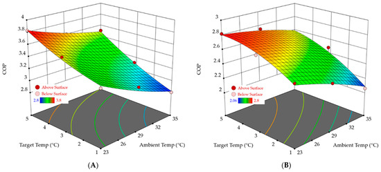
Figure 16.
Average daily COP of the solar-powered refrigerator (SPDR) with a modified ANN-based control system: (A) MR and the SPDR with a traditional control system, (B) TR against the target product temperature and ambient temperature.
For a 1 °C product temperature and 29 °C average daily temperature, the refrigeration system COP was about 3.12 and 1.91 for the MR and TR, respectively. At a 3 °C product temperature and 29 °C average daily temperature, the refrigeration system COP was about 3.28 and 2.30 for the MR and TR, respectively. While at a 5 °C product temperature and 29 °C average daily temperature, the refrigeration system COP was about 3.61 and 2.65 for the MR and TR, respectively.
While at a 1 °C product temperature and 35 °C average daily temperature, the refrigeration system COP was about 2.8 and 2.06 for the MR and TR, respectively. At a 3 °C product temperature and 35 °C average daily temperature, the refrigeration system COP was about 3.11 and 2.52 for the MR and TR, respectively. For a 5 °C product temperature and 35 °C average daily temperature, the refrigeration system COP was about 3.51 and 2.66 for the MR and TR, respectively.
At the average daily temperature of 23 °C, the COP of the MR was higher than the TR by 24.92, 25.07, and 26.37% at a product temperature of 1, 3, and 5 °C, respectively. At the average daily temperature of 29 °C, the COP of the MR was higher than the TR by 38.78, 29.88, and 26.59% at a product temperature of 1, 3, and 5 °C, respectively. While at the average daily temperature of 35 °C, the COP of the MR was higher than the TR by 26.43, 18.97, and 24.22% at a product temperature of 1, 3, and 5 °C, respectively.
Hamad et al. [42] investigated 3 different vapor injection mass ratios (2, 3, and 4%) with variable compression speeds for the frequency range from 35 to 60 Hz. Their findings demonstrated that reducing the compressor speed to 35 Hz resulted in a 36% improvement in the COP and an 18% reduction in the power consumption compared to a conventional refrigeration system. The results obtained in their study agree with the results obtained in the current study. The utilization of a variable speed compressor has had a notable impact on improving the system performance. At a frequency of 35 Hz, it has resulted in an 18% improvement in the COP and a 36.4% reduction in power consumption. Contrarily, increasing the compressor speed to 60Hz has led to a 29% reduction in the COP. In addition, significant savings in power consumption (36%) and an increase in the COP (75%) are observed at a speed of 35Hz, compared to a conventional system [46].
3.5.6. Time Required to Reach the Product Target Temperature
Figure 17 shows the average time required to cool the product from the initial temperature to the targeted temperature for the modified refrigerator (Figure 17A) and traditional refrigerator (Figure 17B) at different ambient temperatures.
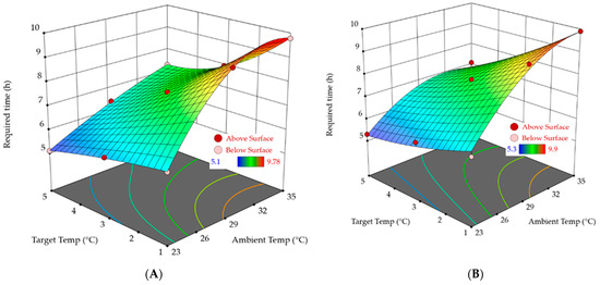
Figure 17.
Average daily time required to cool the product from the initial temperature to the targeted temperature for the solar-powered refrigerator (SPDR) with a modified ANN-based control system: (A) MR and the SPDR with a traditional control system, (B) TR at different ambient temperatures.
At the average daily ambient temperature of 23 °C, the time required to cool the product from the initial temperature of 23 °C to the product temperature of 1 °C was 6.3 h and 6.3 h for the MR and TR, respectively. At the average daily ambient temperature of 23 °C, the time required to cool the product from the initial temperature of 23 °C to the product temperature of 3 °C was 5.8 h and 5.9 h for the MR and TR, respectively. At the same ambient temperature, the time required to reach the product temperature of 5 °C was 5.3 h for both the MR and TR.
For the average ambient temperature of 29 °C and to reach the product temperature of 1 °C, 3 °C, and 5 °C, the time required was 9.33 h, 7.49 h, and 6.9 h for the MR, respectively. Meanwhile, for the TR, the required time was 9.2 h, 7.8 h, and 6.5 h for the product temperature of 1 °C, 3 °C, and 5 °C, respectively.
When the average ambient temperature was 35 °C and to reach the product temperature of 1 °C, 3 °C, and 5 °C, the time required was 9.78 h, 7.97 h, and 7.2 h for the MR, respectively. Meanwhile, for the TR, the required time was 9.9 h, 7.9 h, and 7.1 h for the product temperature of 1 °C, 3 °C, and 5 °C, respectively.
Generally, with the same ambient temperature and refrigerator, increasing the intended product temperature from 1 to 5 °C led to a decrease in the running time of the refrigerator. The statistical analysis revealed that the MR takes more time to reach the product temperature than the TR, but this increase in the time was not significant (p < 0.05%—one-way ANOVA). Even though the MR takes more time than the TR to reach the product temperature, the total energy consumption by the MR was lower than the TR because the MR runs for more time at the lower temperature near the set temperature.
4. Conclusions
Maintaining the product temperature and ensuring energy savings are extremely important. The current study presented an ANN-based control system used to optimize the performance of the display refrigerator powered by a stand-alone PV system. Two different operating control modes were implemented and investigated. They were a traditional control system using a digital temperature controller with a fixed compressor speed (60 Hz) and an ANN-based intelligent control system for controlling the variable compressor speed (40 to 60 Hz) and fan operation. The solar PV system was installed outdoors, and its performance was evaluated. The two control mechanisms were evaluated at three targeted temperatures of 1, 3, and 5 °C when the average ambient temperatures were 23 °C, 29 °C, and 35 °C, respectively. The SPDR was operated under variable frequencies from 40 to 60 Hz. The findings of this investigation are as follows:
- The average daily power of the solar PV system was about 1.098 kW which is enough to overcome the running time of the display refrigerator. The average daily conversion efficiency of the PV modules was about 11.47%.
- The ANN-based regression model was developed based on a training dataset with the designed parameters. Finally, the developed ANN-based model was deployed on an Arduino board to control the frequency for the performance optimization of the SPDR.
- Increasing the ambient temperature caused an increase in the running time of the refrigerator, and hence an increase in the average daily performance.
- At a target product temperature of 5 °C, the MR saved power of about 32.9%, 33.4%, and 35.5% compared to the TR at the average ambient temperature of 23 °C, 29 °C, and 35 °C, respectively.
- The average daily fan power consumption of the MR was significantly lower than the TR under the same tested conditions.
- At a target product temperature of 5 °C, the COP of the MR was higher than the TR by about 26.37%, 26.59%, and 24.22% at an average daily ambient temperature of 23 °C, 29 °C, and 35 °C, respectively.
- The solar PV system helps operate refrigerators away from the electricity grid in rural areas.
- The developed control system performed well and operated the display refrigerator more smoothly than the traditional one.
- The developed control system is expected to provide the basis for designing and optimizing the PV-powered refrigeration system.
This study demonstrated the effectiveness of using an ANN-based regression model to optimize SPDRs. This approach can be applied to other refrigeration systems, providing a more efficient and reliable means of control. However, although machine learning considers an effective tool for optimizing solar-powered refrigerators, accurately modeling for the performance degradation of PV system components, such as PV panels and batteries, is essential for achieving long-term efficiency and reliability. This modeling can be performed through a comprehensive approach that combines ML techniques with accurate degradation models. In addition, future studies are needed to evaluate the influence of this optimized solar-powered display refrigerator with the developed ANN control system on cold-preserved vegetables and fruits.
Author Contributions
Conceptualization, M.M., M.A.E. and N.M.A.; methodology, M.M. and M.A.E.; software, M.M.; validation, M.M., M.A.E. and N.M.A.; formal analysis, M.M.; investigation, M.M. and M.A.E.; resources, M.A.E., M.M. and N.M.A.; data curation, M.M. and M.A.E.; writing—original draft preparation, M.M., M.A.E. and N.M.A.; writing—review and editing, M.M., M.A.E. and N.M.A.; visualization, M.M.; project administration, M.A.E.; funding acquisition, M.A.E., M.M. and N.M.A. All authors have read and agreed to the published version of the manuscript.
Funding
This work was supported by the Deputyship for Research and Innovation, Ministry of Education in Saudi Arabia (Grant No. INST015).
Institutional Review Board Statement
Not applicable.
Informed Consent Statement
Not applicable.
Data Availability Statement
The data are available upon request from the corresponding author.
Acknowledgments
The authors extend their appreciation to the Deputyship for Research and Innovation, Ministry of Education in Saudi Arabia, for funding this research work (Project number INST015).
Conflicts of Interest
The authors declare no conflict of interest.
References
- Noro, M.; Lazzarin, R.M. Solar Cooling between Thermal and Photovoltaic: An Energy and Economic Comparative Study in the Mediterranean Conditions. Energy 2014, 73, 453–464. [Google Scholar] [CrossRef]
- Gao, Y.; Ji, J.; Guo, Z.; Su, P. Comparison of the Solar PV Cooling System and Other Cooling Systems. Int. J. Low-Carbon Technol. 2018, 13, 353–363. [Google Scholar] [CrossRef]
- Ayadi, O.; Al-Dahidi, S. Comparison of Solar Thermal and Solar Electric Space Heating and Cooling Systems for Buildings in Different Climatic Regions. Sol. Energy 2019, 188, 545–560. [Google Scholar] [CrossRef]
- Li, N.; Uckun, C.; Constantinescu, E.M.; Birge, J.R.; Hedman, K.W.; Botterud, A. Flexible Operation of Batteries in Power System Scheduling with Renewable Energy. IEEE Trans. Sustain. Energy 2016, 7, 685–696. [Google Scholar] [CrossRef]
- Rowe, M.; Yunusov, T.; Haben, S.; Holderbaum, W.; Potter, B. The Real-Time Optimisation of DNO Owned Storage Devices on the LV Network for Peak Reduction. Energies 2014, 7, 3537–3560. [Google Scholar] [CrossRef]
- Sabry, A.H.; Ker, P.J. DC Environment for a Refrigerator with Variable Speed Compressor; Power Consumption Profile and Performance Comparison. IEEE Access 2020, 8, 147973–147982. [Google Scholar] [CrossRef]
- Dhondge, A.J.; Kalbande, S.R. Performance Evaluation of Solar Photovoltaic Powered Vapor Compression Refrigeration System. Int. J. Agric. Sci. 2018, 10, 6651–6653. [Google Scholar]
- Kasali, A.A.; Olaleye, J.O.; Lukmon, B.-F.; Salami, F.; Opeyemi. The Design and Development of a Solar-Powered Picnic Refrigerator. J. Sci. Eng. Res. 2020, 2020, 44–52. [Google Scholar]
- Eltawil, M.A.; Samuel, D.V.K. Vapour Compression Cooling System Powered By Solar PV Array for Potato Storage. Agric. Eng. Int. CIGR J. 2007, 9, 1–23. [Google Scholar]
- Makinde, K.; Man Alhaji Sulaiman, A.E. Design and Fabrication of Solar Powered Mobile Cold Room. International Journal of Trend in Scientific Research and Development. IJTSRD Int. J. Trend Sci. Res. Dev. 2019, 3, 342–350. [Google Scholar]
- Selvaraj, D.A.; Victor, K. Design and Performance of Solar PV Integrated Domestic Vapor Absorption Refrigeration System. Int. J. Photoenergy 2021, 2021, 6655113. [Google Scholar] [CrossRef]
- Mohammed, M.; Riad, K.; Alqahtani, N. Design of a Smart IoT-Based Control System for Remotely Managing Cold Storage Facilities. Sensors 2022, 22, 4680. [Google Scholar] [CrossRef] [PubMed]
- Ekren, O.; Yilanci, A.; Cetin, E.; Ozturk, H.K. Experimental Performance Evaluation of a PV-Powered Refrigeration System. Elektronika ir Elektrotechnika 2011, 8, 7–10. [Google Scholar] [CrossRef]
- Arora, C.P. Refrigeration and Air Conditioning, 2nd ed.; Tata McGraw-Hill Publishing Company Limited: New Delhi, India, 2000. [Google Scholar]
- Espíndola, R.S.; Knabben, F.T.; Melo, C.; Hermes, C.J.L. Thermal Performance of Skin-Type, Hot-Wall Condensers, Part II: Design Guidelines for Household Applications. Int. J. Refrig. 2020, 110, 262–267. [Google Scholar] [CrossRef]
- Agarwal, S. Thermodynamic Performance Analysis of Dedicated Mechanically Subcooled Vapour Compression Refrigeration System. J. Therm. Eng. 2019, 5, 222–233. [Google Scholar] [CrossRef]
- Long, R.; Li, B.; Liu, Z.; Liu, W. Performance Analysis of a Solar-Powered Electrochemical Refrigerator. Chem. Eng. J. 2016, 284, 325–332. [Google Scholar] [CrossRef]
- Dupont, J.L.; Domanski, P.; Lebrun, P.; Ziegler, F. The Role of Refrigeration in the Global Economy. In Proceedings of the 38th Note on Refrigeration Technologies, IIF-IIR, Paris, France, 1 June 2019; Volume 29, p. 12. [Google Scholar] [CrossRef]
- Dincer, I. (Ed.) Refrigeration Systems and Applications; John Wiley & Sons: Hoboken, NJ, USA, 2017; ISBN 9781119230755. [Google Scholar]
- Shweta, A.S. Intelligent Refrigerator Using Artificial Intelligence. In Proceedings of the 2017 11th International Conference on Intelligent Systems and Control (ISCO), Coimbatore, India, 5–6 January 2017; pp. 464–468. [Google Scholar]
- Pérez-Gomariz, M.; López-Gómez, A.; Cerdán-Cartagena, F. Artificial Neural Networks as Artificial Intelligence Technique for Energy Saving in Refrigeration Systems—A Review. Clean Technol. 2023, 5, 116–136. [Google Scholar] [CrossRef]
- Mohammed, M.; Munir, M.; Aljabr, A. Prediction of Date Fruit Quality Attributes during Cold Storage Based on Their Electrical Properties Using Artificial Neural Networks Models. Foods 2022, 11, 1666. [Google Scholar] [CrossRef]
- Mohammed, M.; Hamdoun, H.; Sagheer, A. Toward Sustainable Farming: Implementing Artificial Intelligence to Predict Optimum Water and Energy Requirements for Sensor-Based Micro Irrigation Systems Powered by Solar PV. Agronomy 2023, 13, 1081. [Google Scholar] [CrossRef]
- Belman-Flores, J.M.; Rodríguez-Valderrama, D.A.; Ledesma, S.; García-Pabón, J.J.; Hernández, D.; Pardo-Cely, D.M. A Review on Applications of Fuzzy Logic Control for Refrigeration Systems. Appl. Sci. 2022, 12, 1302. [Google Scholar] [CrossRef]
- Al-Aifan, B.; Parameshwaran, R.; Mehta, K.; Karunakaran, R. Performance Evaluation of a Combined Variable Refrigerant Volume and Cool Thermal Energy Storage System for Air Conditioning Applications. Int. J. Refrig. 2017, 76, 271–295. [Google Scholar] [CrossRef]
- Ko, J.-S.; Huh, J.-H.; Kim, J.-C. Improvement of Energy Efficiency and Control Performance of Cooling System Fan Applied to Industry 4.0 Data Center. Electronics 2019, 8, 582. [Google Scholar] [CrossRef]
- Lee, D.; Tsai, F.-P. Air Conditioning Energy Saving from Cloud-Based Artificial Intelligence: Case Study of a Split-Type Air Conditioner. Energies 2020, 13, 2001. [Google Scholar] [CrossRef]
- Raghunatha Reddy, D.V.; Bhramara, P.; Govindarajulu, K. A Comparative Study of Multiple Regression and Artificial Neural Network Models for a Domestic Refrigeration System with a Hydrocarbon Refrigerant Mixtures. Mater. Today Proc. 2020, 22, 1545–1553. [Google Scholar] [CrossRef]
- Mohammed, M.; Munir, M.; Ghazzawy, H.S. Design and Evaluation of a Smart Ex Vitro Acclimatization System for Tissue Culture Plantlets. Agronomy 2022, 13, 78. [Google Scholar] [CrossRef]
- Mohammed, M.; Riad, K.; Alqahtani, N. Efficient Iot-Based Control for a Smart Subsurface Irrigation System to Enhance Irrigation Management of Date Palm. Sensors 2021, 21, 3942. [Google Scholar] [CrossRef]
- ASU Arizona State University. Solar PV Stand-Alone Systems, Good Practice Guide: Small System Sizing; AZ, USA. Available online: https://cfo.asu.edu/solar (accessed on 19 February 2023).
- Koutroulis, E.; Kolokotsa, D. Design Optimization of Desalination Systems Power-Supplied by PV and W/G Energy Sources. Desalination 2010, 258, 171–181. [Google Scholar] [CrossRef]
- Wu, C. Maximum Obtainable Specific Cooling Load of a Refrigerator. Energy Convers. Manag. 1995, 36, 7–10. [Google Scholar] [CrossRef]
- Chen, L.; Wu, C.; Sun, F. Heat Transfer Effect on the Specific Cooling Load of Refrigerators. Appl. Therm. Eng. 1996, 16, 989–997. [Google Scholar] [CrossRef]
- Göktun, S. Coefficient of Performance for an Irreversible Combined Refrigeration Cycle. Energy 1996, 21, 721–724. [Google Scholar] [CrossRef]
- Kirkup, L.; Frenkel, R.B. An Introduction to Uncertainty in Measurement Using the Gum (Guide to the Expression of Uncertainty in Measurement); Cambridge University Press: Cambridge, UK, 2006; pp. 1–233. ISBN 9780511755538. [Google Scholar] [CrossRef]
- Lira, I. Evaluating the Measurement Uncertainty: Fundamentals and Practical Guidance. Metrologia 2003, 40, 207. [Google Scholar] [CrossRef]
- Imara, Z.M.; Eltawil, M.A. Performance of Small Scale Spv-Powered-Drip Irrigation System for Remote Regions. Misr J. Agric. Eng. 2006, 23, 1133–1154. [Google Scholar]
- Fernoaga, V.; Sandu, V.; Balan, T. Artificial Intelligence for the Prediction of Exhaust Back Pressure Effect on the Performance of Diesel Engines. Appl. Sci. 2020, 10, 7370. [Google Scholar] [CrossRef]
- Wright, L.G.; Onodera, T.; Stein, M.M.; Wang, T.; Schachter, D.T.; Hu, Z.; McMahon, P.L. Deep Physical Neural Networks Trained with Backpropagation. Nature 2022, 601, 549–555. [Google Scholar] [CrossRef]
- Gao, Y.; Ji, J.; Han, K.; Zhang, F. Comparative Analysis on Performance of PV Direct-Driven Refrigeration System under Two Control Methods. Int. J. Refrig. 2021, 127, 21–33. [Google Scholar] [CrossRef]
- Hamad, A.J.; Khalifa, A.H.N.; Khalaf, D.Z. The Effect of Compressor Speed Variation and Vapor Injection on the Performance of Modified Refrigeration System. Int. Rev. Mech. Eng. 2018, 12, 285–292. [Google Scholar] [CrossRef]
- Chu, C.M.; Jong, T.L.; Huang, Y.W. Thermal Comfort Control on Multi-Room Fan Coil Unit System Using LEE-Based Fuzzy Logic. Energy Convers. Manag. 2005, 46, 1579–1593. [Google Scholar] [CrossRef]
- Moria, H.; Ahmed, M.; Alghanmi, A.; Mohamad, T.I.; Yaakob, Y. Experimental Study of Solar Based Refrigerator Using Thermoelectric Effect. Energy Procedia 2019, 158, 198–203. [Google Scholar] [CrossRef]
- Rajoria, C.S.; Singh, D.; Gupta, P.K. Performance Evaluation of Solar Photovoltaic Panel Driven Refrigeration System. IOP Conf. Ser. Mater. Sci. Eng. 2018, 330, 012133. [Google Scholar] [CrossRef]
- Hamad, A.J.; Khalifa, A.H.N.; Khalaf, D.Z. Performance Investigation of Vapor Compression Cycle with a Variable Speed Compressor and Refrigerant Injection. J. Mech. Eng. 2019, 16, 63–76. [Google Scholar] [CrossRef]


Disclaimer/Publisher’s Note: The statements, opinions and data contained in all publications are solely those of the individual author(s) and contributor(s) and not of MDPI and/or the editor(s). MDPI and/or the editor(s) disclaim responsibility for any injury to people or property resulting from any ideas, methods, instructions or products referred to in the content. |
© 2023 by the authors. Licensee MDPI, Basel, Switzerland. This article is an open access article distributed under the terms and conditions of the Creative Commons Attribution (CC BY) license (https://creativecommons.org/licenses/by/4.0/).