Application of Artificial Intelligence Model Solar Radiation Prediction for Renewable Energy Systems

Abstract

Solar power is an excellent alternative power source that can significantly cut our dependency on nonrenewable and destructive fossil fuels. Solar radiation (SR) can be predicted with great precision, and it may be possible to drastically minimize the impact cost associated with the development of solar energy. To successfully implement solar power, all projects using solar energy must have access to reliable sun radiation data. However, the deployment, administration, and performance of photovoltaic or thermal systems may be severely impacted by the lack of access to and the ambiguity of this data. Methods for estimating and predicting solar radiation can help solve these problems. Prediction techniques can be put to use in the real world to, for example, keep the power grid functioning smoothly and ensure that the supply of electricity exactly matches the demand at all times. Recently developed forecasting methods include the deep learning convolutional neural networks combined with long short-term memory (CNN-LSTM) model. This study provides a comprehensive examination of meteorological data, along with the CNN-LSTM methods, in order to design and train the most accurate SR forecasting artificial neural network model possible. Weather data was collected from a NASA meteorological station that included details such as the current temperature, the relative humidity, and the speed of the wind. This research revealed that SR is highly correlated with both temperature and radiation. Furthermore, the findings demonstrated that the CNN-LSTM algorithm outperformed the other algorithm-trained models, as evidenced by the performance score of the respective models, with a maximum coefficient determination (R²) > 95% and a minimum mean square error (MSE) of 0.000987 at the testing step. In comparison with different existing artificial intelligence models, the CNN-LSTM model outperformed the other models. These scenarios demonstrated that a basic implementation of CNN-LSTM can be used to supplement conventional methods for predicting SR, provide possibilities to monitor radiation at a low cost, and encourage the adoption of data-driven management.

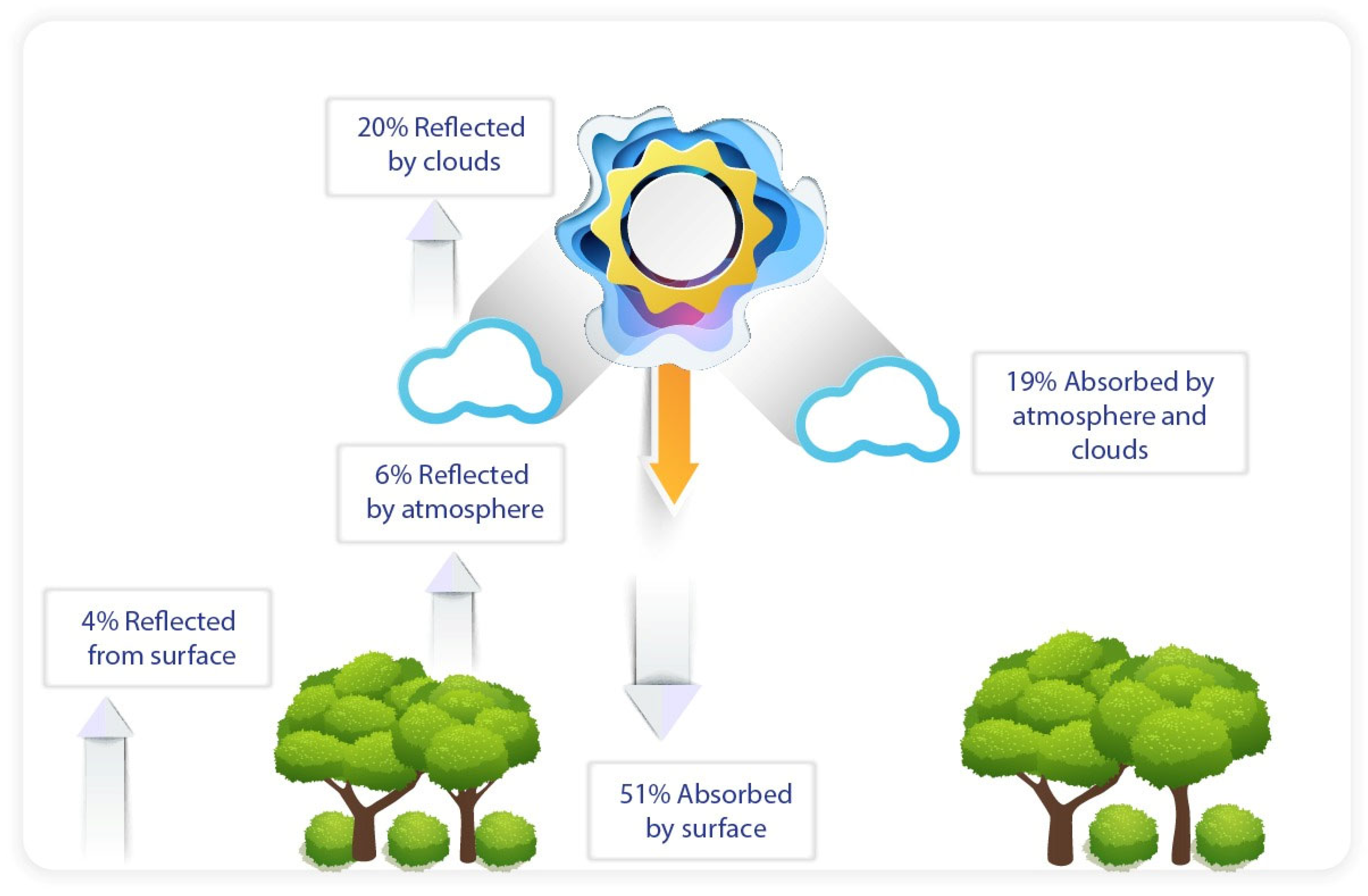
1. Introduction

The quantity of energy that humans receive from the sun can only be considerably changed by three spheres: the atmosphere, the biosphere, and the hydrosphere [1]. Changes in solar radiation (SR) have a significant impact at a global scale because even small variations in SR can produce significant variations in the weather on Earth [2]. In particular, the ocean is affected, which may result in catastrophic occurrences, such as the Nino–Southern Oscillation [3,4]. For the purpose of advancing scientific research in the disciplines of solar energy, building materials, and climatic extremes, accurate measurements and analyses of the temporal and geographical variability of SR are vital [2,5]. Figure 1 shows the distribution of solar radiation on Earth.

As a result of rising temperatures, a deteriorating human ecological environment, a lack of readily available nonrenewable energy sources, and widespread pollution, the use of solar photovoltaic power as a means of generating electricity has seen a tremendous increase in recent years all over the globe. Large-scale grid connections, on the other hand, have a negative impact on the dependability and safety of the energy system, and they can also result in considerable economic losses [6,7]. Accurately predicting the amount of electricity that will be generated by the sun is an essential first step in the process of power dispatching, which is the most important factor in boosting the amount of electricity that is generated by photovoltaic cells inside the power system. Nevertheless, variations in the radiation of the sun are the principal cause of differences in the amount of electricity produced by photovoltaic cells. As a consequence of this, it is of the highest significance to provide accurate forecasts of solar irradiance, since these predictions may serve as useful decision-making aids for power dispatching systems and assist in the reduction of operating costs connected with the power system [8].

The expanding human population in our contemporary world is very reliant on the availability of energy in order to carry out day-to-day activities and satisfy human requirements. Renewable energy sources, particularly solar energy, have the potential to satiate the world’s need for electricity while simultaneously lowering the amount of heat generated by traditional sources. Irradiance from the sun is an important factor to consider when discussing solar power applications. The availability of solar irradiance is impacted by a number of elements, including predicting horizon, weather categorization, and performance assessment measures, all of which should be taken into account. When it comes to the effective administration of solar energy systems, having an accurate estimate of the amount of solar irradiation is of the highest significance for both the power system designers and the grid operators. Due to the fact that solar irradiance is intermittent and does not remain stable over time, many of the statistical and machine learning algorithms that are now in use are less capable of making accurate forecasts. Some researchers in this field suggested the idea of using deep learning models as a means of improving prediction accuracy and mitigating some of the drawbacks associated with conventional machine learning models [9].

In recent years, there has been an increase in the number of novel techniques and algorithms that can anticipate SR. Empirical models, theoretical parameter-based techniques, and models that use machine learning (ML) and artificial intelligence (AI) technologies to draw on information from ground-based weather stations or satellites are all included in this category of models [10,11]. There are a number of ML models, such as artificial neural networks and random forest, that have been successfully applied to the prediction of SR. This success can be attributed to the fact that these models are able to successfully learn from data and make predictions. For instance, Alawi et al. [12], Mohandas et al. [13], Reddy et al. [14], and Yildiz et al. [15] employed artificial neural networks to predict SR in Oman, Saudi Arabia, India, and Turkey, respectively. Deep learning is a subfield of ML which, in comparison to artificial neural networks and other types of machine learning, has a more robust learning capacity and calls for an increased amount of data in order to attain improved prediction accuracy [16,17].

In this piece of work, a detailed and all-encompassing analysis of deep learning-based solar irradiance forecasting models is provided for consideration. The performance and usefulness of a number of different deep learning models, such as long-term memory and the convolution neural network, have been proposed. The main motivation of the developing prediction system is to benefit the Kingdom of Saudi Arabia, which enjoys strong elements in the field of solar energy and wind energy, due to its location within the “global solar belt”. Therefore, developing a model based on artificial intelligence technology is very important to predict solar radiation. The main contributions of the proposed work are as follows:

• Generally, this work assists in achieving several of the United Nation Sustainable Development Goals. It is directly aligned with Goal No. 7, “Affordable and Clean Energy”, and it is indirectly helping to achieve other goals as well.
• Specifically, in this work, a highly efficient artificial intelligence (AI) model has been developed to predict solar radiation and thus estimate the power production of photovoltaic systems.
• The developed model incorporates sensitivity analysis as a new tool to analyze the average RS and to obtain datasets of the sunrise and sunset.
• Compared to the available models, the current model shows superior performance in predicting solar radiation.

2. Literature Review

This section provides a comprehensive overview of the many different kinds of machine learning techniques that may be used to predict a solar radiation variable. Pang et al. [18] used the recurrent network method in their research, enabling them to create a recurrent neural network (RNN). In order for the scientists to make estimates of solar radiation, they loaded the computer with meteorological data from Alabama. The RNN and the multilayer perceptron (MLP) were evaluated next to one another for comparison. Inputs such as radiation and temperature were exploited in order to establish an external variable, such as the time of day. The prediction models were able to reach R = 0.983, while only having an RMSE = 41. They recommended including variables, such as cloud cover, in the control models, which may influence forecasts. Zhu et al. [19] conducted research in which they compared the LSTM approach to a CNN. In their inquiry, rather than depending on more conventional historical data, they chose to make use of images instead. The RMSE was 29.92%, while the efficacy of the prediction was found to be 0.93%. The fact that photos may provide useful results, even when the conditions are less than perfect, is one of the most significant advantages of using images. Shamshirband et al. [20] examined a variety of algorithms that make use of ANN and compared and contrasted them. They observed a number of disadvantages, some of which are as follows: MLP-based networks are not particularly successful when dealing with time series applications. Despite the limitations of LSTM networks, they are becoming more popular in prediction work due to the enhanced robustness of these networks. Tree-based methods are very popular due to the ease with which they can be implemented and the flexibility with which they may adjust their predictive accuracy via the modification of various hyperparameters. Meng et al. [21] predicted the RS in Xingtai City, which is located in northern China, for three distinct kinds of meteorological conditions: clear sky, clouds, and rain. The predictions were made using an random forest (RF) algorithm. The ultimate conclusions were obtained by averaging the results of all of the regressions performed on the datasets. According to the findings of a study conducted by Lee et al. [22], which looked at two different machine learning tree models, namely RF and boosted for forecasting RS, and these models achieved significantly better results than the support vector machine (SVM) method and the Gaussian regression technique (R = 97%, RMSE = 59.27). The data from 16 stations were used in this analysis. Even though they came to the conclusion that tree-based models performed well, they made the observation that no one model emerged as the undisputed victor. In addition to machine learning, hybrid algorithms may also combine aspects of other kinds of algorithms, such as metaheuristic or optimization algorithms. Eseye et al. [23] developed a system based on wavelet-PSO-SVM by merging data obtained from meteorological sources with those obtained from statistical models. Using a dataset that was divided into four pieces—one for each of the four seasons—the following calculation was performed: when looking at a time horizon of three hours, the RMSE is 0.73 during the winter, 0.76 during the spring, 1.024 during the summer, and 0.8598 during the winter. According to these results, this strategy is beneficial for constructing models of predictions with a relatively limited time horizon.

Feng et al. [24] developed the SolarNet model in order to automatically extract the characteristics of a complete sky picture. In order to combine many images and historical values, Zhao et al. [25] built a 3D-CNN model, which they then sent into a multilayer perceptron as input. This allowed them to successfully complete the task (MLP). On the other hand, a typical neural network structure, in addition to an MLP, is unable to store the LSTM of an input time series, since the nodes between the hidden layers of ANN are not connected. For this reason, when attempting to anticipate a time series, the use of MLPs is not very helpful. An LSTM is a kind of memory that incorporates a complex memory unit that may retrieve data from the past and utilize it in the process of computing output at the current time; in other words, the nodes between buried layers can become linked [26]. When it comes to predicting a time series, an LSTM performs better than an MLP; hence, it stands to reason that an LSTM is the superior model. The time series learning capabilities of LSTM networks [27,28], which have been used in the process of forecasting solar irradiance, are very helpful for this purpose. These networks have been put to use in the process. This study improved on prior work by addressing the shortcomings in the aforementioned model through developing a CNN-LSTM model. This model was created to solve the flaws in the aforementioned model. Using a Siamese CNN, it is possible to automatically extract the spatial aspects of a large number of continuously taken, complete sky images, while maintaining the ability to retain the temporal features. A concatenate layer is then used to mix the data from the meteorological records and the image. This combined data is then delivered into the LSTM in order to predict the solar irradiance that will occur during the next few hours.

As a result of developments in technology over the last several decades [29,30,31], the use of AI has become more widespread across almost all technical fields. Predictions of solar radiation data were made using a variety of artificial intelligence techniques, including support vector regression (SVR), kernel nearest neighbors (k-NNs), deep learning (DL), and ANNs [32,33]. Applications of AI may benefit greatly by identifying the DL hyperparameters that can be used to narrow the search space and then afterwards implementing hyperparameter optimization [34,35]. When it comes to estimating solar radiation, an earlier study has demonstrated that AI models provide more accuracy. This paper [36] provides a model for predicting solar irradiance by combining particle swarm optimization and least squares support vector regression. The authors found that using LightGBM and CatBoost, their model for forecasting solar irradiance showed significant improvement in performance [37,38,39]. LightGBM provided better performance matrices than other AI systems, such as SVR and multiple linear regression (MLR). Many feasibility studies show that, if accurate projections of solar irradiance can be made, Bangladesh has a great deal of potential to meet its electric power demand via the deployment of a solar–wind hybrid system [40,41].

3. Materials and Methods

In this research, the global database from NASA Meteoblue was collected in order to obtain information. These datasets provide the meteorological information that was collected at the HI-SEAS weather station during the period of time between Mission IV and Mission V (September 2016 to December 2016). We analyzed the data in order to make accurate forecasts about the solar radiation. The completed dataset contains a total of 32,686 samples for each parameter. This means that while 80% of the data will be used for training the model, the other 20% will be used as a “test subset” to make predictions about solar radiation. The conceptual foundation of solar radiation forecasting is shown in Figure 2.

3.1. Dataset

The information for this dataset was collected from Kaggle, where it was posted as a standard dataset. It includes readings from the previous four months, and a prediction about the amount of solar radiation is required. These files provide the meteorological information collected at the HI-SEAS weather station during the period of time between Mission IV and Mission V (September 2016 to December 2016). The features of the dataset are presented in

Table 1. Significant parameters.

Parameters	Features
Date	yyyy-mm-dd format
Time	hh:mm:ss 24 h format
Solar radiation	watts per m2
Temperature	degrees Fahrenheit
Humidity	percent
Barometric pressure	Hg
Wind direction	degrees
Wind speed	miles per hour
Sunrise/sunset	Hawaii time

.

3.2. Data Normalization

Normalizing the data is a necessary step that must be taken before any of the deep learning models described in this article can make use of the information. The goal is to remove the impact of the feature attribute dimension in the data on the model in order to speed up the convergence of the model and increase the model’s predicted accuracy. We use the max-min normalization approach in the study, which is as follows:

$$z_n=\frac{x-x_{min}}{x_{max-x_{min}}},$$

(1)

The normalized data are denoted by the symbol $z_n$, the current observation data are denoted by the letter $x$, and the highest and lowest values in the current observation data are denoted by the symbols $x_{max}$ and $x_{min}$, respectively.

3.3. Prediction Models

3.3.1. A Convolutional Neural Network (CNN)

A CNN is a type of neural network that processes comparable gridded input more efficiently than other types of neural networks. CNNs, which are distinguished by their weight sharing and local connection properties, have made significant contributions to the area of deep learning and have found widespread use in a variety of contexts. The convolutional layer is responsible for the majority of the work necessary to accomplish the CNN’s primary goal, which is to extract feature information from the input. Input data often exhibits nonlinear properties because the feature information retrieved by the convolutional layer is linear. Therefore, implementing a nonlinear function is required in order to achieve success in resolving this issue. The activation function of the CNN is represented by this particular nonlinear function. The CNN model demonstrates the convolution operation, a two-dimensional discrete convolution is utilized as a model, and in order to demonstrate the activation function, the Relu function is used as an example. The precise procedure is described as follows:

$$H\left(i,j\right)=\left(I\ast k\right)\left(i,j\right)={\sum }_m{\sum }_{n}k\left(m,n\right)I(i+m,j+n)$$

(2)

$$f\left(x\right)=\mathrm{m}\mathrm{a}\mathrm{x}(0,x)$$

(3)

where $H\left(i,j\right)$ is a place in the feature map that has been convolutionally altered and indicates a particular location. The size of the input array $x$, denoted by $i$, and the convolution kernel, denoted by $k\left(m,n\right)$ both have their own unique symbols. After the convolution procedure, the feature map, which is often a tensor, is denoted by the letter x. According to the formula that was just shown, the convolution kernel is able to glide across the input array. As it moves to a new location, the items of the array that correspond to that position are multiplied and added together. At long last, the feature map matrix will be acquired when the sliding input array has been finished in its entirety. The feature information that was recovered by the convolution procedure is represented by each individual element of the feature map. In the last step, the feature map is introduced into the activation function in order to provide it with nonlinear properties. This boosts the expressive capacity of the whole network and plays an essential part in the process of data fitting. Figure 3 displays a typical representation of a CNN model’s internal organization.

3.3.2. Long Short-Term Memory (LSTM)

For learning long-term dependencies from time series data, the LSTM neural network is an effective tool. The LSTM model was first introduced in the year 1997 [42], and it is now being used in a broad number of applications within the field of time series forecasting [43]. In point of fact, LSTM is a version of the recurrent neural network. This variant overcomes the issue of gradient disappearance that occurs during the usual training process for RNNs, and as a result, it is able to maintain long-term information. Figure 4 depicts the LSTM algorithm’s underlying structure, for clarity.

The LSTM is a specialized kind of RNN. The most significant departure from the conventional RNN is the incorporation of the idea of memory cells into the model. Since it contains memory cells, LSTM is endowed with the capacity to remember information from the input sequence for an extended period of time. In Figure 4, the symbol $C_t$ serves as a depiction of memory cells. At this point, the LSTM decides whether or not to update or forget the cell state by using a variety of gates. To be more specific, there are three distinct varieties of LSTM inputs at time $t$. These include the input xt at the present time, the state of the hidden layer at time $h_t,$ and the state of the cell at time $C_t$ from the time before. Output gate $o_t$ is used to identify the current hidden layer state h_t, while the forget gate f_t and input gate i_t are used to regulate which information is fed to the cell state. The output gate $o_t$ is used to control which information should be added to the cell state. The current cell state, denoted by $C_t$, and the state of the hidden layer, denoted by $h_t$, are the LSTM’s final outputs. The following is the formula for the particular gating unit:

$$f_t=\sigma \left(W_f·X_t+W_f{·h}_{t-1}+b_f\right)$$

(4)

$$i_t=\sigma (W_c{·X}_t+W_i{·h}_{t-1}+b_i)$$

(5)

$$o_t=\sigma (W_o+X_t+W_o{·h}_{t-1}+V_o·C_t+b_o)$$

(6)

where $X_t$ and $h_t$ denote that the network is given both the sequence data and the hidden layer, at the same time as an input. The network has matching parameters denoted by the letters $W_f,$ $W_i$, and W_o, as well as b_f, b_i, and b_o. To be more specific, the weighted coefficient matrices that correspond to each gate are denoted by the letters $W_f,$ $W_i$, and $W_o$, whereas the letters $b_f$, $b_i$, and $b_o$ indicate the offsets. Each gate has a sigmoid activation function denoted by the symbol. The following describes the method used to update the cell’s status:

$$\stackrel{\_}{c}=\tan h\left(W_c\right[h_{t-1},X_t]+b_c)$$

(7)

$$\mathrm{Cell}\mathrm{gate}:C_t=(f_t\ast C_{t-1}+i_t\ast \tilde{c})$$

(8)

where the * denotes the process of multiplying items that are equivalent. The hyperbolic tangent activation function is denoted by the symbol $\tan h$. The newly modified cell $C_t$ is made up of the value left behind in the cell $C_{t-1}$ after it was processed by the forget gate, as well as the value obtained from the newly inserted cell $C_t$ after the input gate; the $\tilde{c}$ is the candidate for the cell state at the time interval (t). In conclusion, we are able to take advantage of the upgraded cells to produce new hidden states by way of the output gate:

$$\mathrm{Hidden}\mathrm{layer}:h_t=o_t+\tan h\left(C_t\right)$$

(9)

It is the output gate’s responsibility to make certain that the newly concealed state contains no data that is not wholly or substantially legitimate. It is important to point out that, in LSTM, the memory cells are updated by means of addition operations. This allows LSTM to store the cell state for a considerable amount of time and prevents the gradient information from being lost as a result of backpropagation.

Pseudocode of CNN-LSTM

Input: data of SR $D=\left\{\left(x_i,y_i\right)\right|i=1,\dots \dots ..p)$ Output: prediction SR #Parameters: FC: full connected layer, max: maximum pool layer,$\sigma :sigmoidacticationfunction,$ ω:convolution layer, g: computing the size of convolution layer:$i=i+g-1$ $W_o,W_f:$ weight matrix, $b_o$ balance vector and $h_{t-1}$ is hidden layer of cell state. Both $x_t$ and $C_t$ represent the current time’s input and storage units, respectively. $y$: prediction/forecasting values of SR and $y^{\left(i\right)}$ is observation SR data

#Training model:     #At begging: initialization all the significant parameters in CNN-LSTM model      For o in n do:      (1) The features are extraction by using       CNN: $x_i$ =$FC\left\{\mathrm{m}\mathrm{a}\mathrm{x}\right\{\sigma (\omega x{x}_{i:i+g-1}$ $+b\left)\right\}\}$      (2) LSTM fault characteristics from many time segments are combined into one sequential fault model.        Features: $h_t=o_t+\tan h\left(C_t\right)$      (3) The prediction results are generated by a technique that allots the weights to the complete connection layer.        Prediction/forecasting results: $a_t=\sum \sigma \left(\tan h\right(H_t$)) ∗ $h_t$,        $y=FC(W_f·a_t$)      (4) Calculate the training loss values of the CNN-LSTM          $L={\displaystyle \sum _{I=1}^N}{Y}^{\left(i\right)}\log y^{\left(i\right)}+\left(1-y^{\left(i\right)}\right)\mathrm{l}\mathrm{o}\mathrm{g}(1-y^{\left(i\right)})$ # The CNN parameters should be adjusted for obtaining high accuracy End

Step of CNN-LSTM Algorithm for predicting SR

#Define Preprocessing Load the time series dataset Use Min_Max normalization Split the dataset into training and testing sets Define the CNN-LSTM model architecture Train the model on the training data Evaluate the model on the testing data Use the trained model to make predictions on new data #Define CNN-LSTM Model Define the input layer with the shape (n_timesteps, n_features, 1) Define a Conv1D layer with filters, kernel_size, activation function and padding. Define a MaxPooling1D layer to reduce the spatial dimensions Define a LSTM layer with units, activation function, and return_sequences=True Define a Flatten layer to reduce the output dimensions Define a Dense layer with the output size #Compile the model Define the optimizer, loss function and metrics to optimize Compile the model with the above mentioned optimizer, loss function and metrics #Train the model Fit the model on the training data with batch size, epochs and validation data Save the trained model  #Evaluate the model Load the saved model Use the evaluate method to get the loss and metrics on the test data Calculate the prediction values on the test data #Make predictions Load the saved model Use the predict method to make predictions on new data

3.4. Statistical Metrics for Data Validation

The metrics and indicators for assessing prediction models are presented in this section. We include four of the most prominent measures, namely the mean square error (MSE), RMSE, normalized root mean square error (NRMSE), R, and R² collected through a study of prior research. These metrics are considered the most dependable when making predictions.

It is possible that the MSE is the machine learning function that can be computed with the least amount of complexity. It measures a square root of the difference that may be found between the model’s predictions and the actual data, also known as the ground truth, and then applies that average to the whole dataset. The MSE cannot ever express negativity.

$$MSE=\frac{1}{n}{\sum }_{i=1}^n{(y_{i,exp}-y_{i,pred})}^2$$

(10)

The RMSE is a calculation that determines how well a model fits data that is connected to reducing high error rates:

$$RMSE=\sqrt{{\sum }_{i=1}^n\frac{{\left(y_{i,exp}-y_{i,pred}\right)}^2}{n}}$$

(11)

$$R\%=\frac{n\left(\sum _{i=1}^n{y_{i,exp}\times }_{}{y}_{i,pred}\right)-\left(\sum _{i=1}^n{y}_{i,exp}\right)\left(\sum _{i=1}^n{y}_{i,pred}\right)}{\sqrt{\left[n{\left(\sum _{i=1}^n{y}_{i,exp}\right)}^2-{\left(\sum _{i=1}^n{y}_{i,exp}\right)}^2\right]\left[n{\left(\sum _{i=1}^n{y}_{i,pred}\right)}^2-{\left(\sum _{i=1}^n{y}_{i,pred}\right)}^2\right]}}\times 100$$

(12)

$$R^2\%=1-\frac{{\sum }_{i=1}^n({y_{i,exp}-y_{i,pred})}^2}{{\sum }_{i=1}^n({y_{i,exp}-y_{avg,exp})}^2}$$

(13)

where $y_{i,exp}$ represents the actual value of data point $i$, $y_{i,pred}$ represents the predicted value of data point $i$, $y_{avg,exp}$ represents the average of the actual values, and n is the total amount of input data.

4. Sensitivity Analysis

One of the most well-known and often used data-driven methodologies is regression analysis. It is a kind of supervised learning that is commonly applied as a linear regression analysis in the traditional analysis of data, such as that performend on solar radiation data. It is a method of teaching in which the learner is directly monitored by an instructor. It makes it possible to sort the influence of the independent variable (or variables) on the related dependent variable in each particular dataset in a fashion that is both systematic and quantitative. As a result, the importance of the independent variable(s) and the interactions between them in relation to the dependent variable will be determined.

Table 2. Sensitivity analysis results.

	Time	Radiation	Temperature	Pressure	Humidity	Wind Direction	Wind Speed
Coun	3.268600 × 104	32,686.00	32,686.00	32,686.00	32,686.000	32,686.000	32,686.00
Mean	1.478047 × 109	207.124697	51.103	30.422	75.016	143.489	6.243
Std	3.005037 × 106	315.916	6.201	0.054	25.990	83.167	3.49047
Min	1.472724 × 109	1.110	34.000	30.190	8.000	0.0900	0.00
Max	1.483265 × 109	1601.260	1.483265 × 109	71.000	30.560	103.000	40.500

shows the statistical analysis of dataset parameters.

The average of the radiation features presented in Figure 5 is observed, showing that the mean is 210 in the time period 1 September 2016 to 31 December 2016.

Figure 6 shows the radiation in hours and months. It is noted that the radiation increases between the 6 am to 4 pm hours in the three months tested. Since the day is longer in September compared to the other months, the difference in length between dawn and sunset is also larger, as presented in Figure 7. It also seems that higher levels of radiation emerge more often in September. This is a finding that was to be predicted (or, it might just be a statistical issue, since the day is longer, so there is more likelihood of high radiation).

The correlation refers to a statistical metric that may be used to assess or quantify the degree to which two variables are related to one another. The Pearson product–moment correlation is the most used approach, and for good reason: it reveals the linear connection that exists between any two variables. There have been several studies that have shown that just because the Pearson value is equal to zero does not mean that the variables are unrelated to one another. Following the completion of the reading process and any necessary data transformations, the next step is to visualize the results. The construction of a correlation matrix serves as the first stage for determining the nature of the links that exist between the most important variables. Figure 8 and Figure 9 illustrate the correlation coefficients of the solar radiation data at different time periods (monthly, hourly). It is observed that the radiation values have a high correlation with temperature values > 77% at different time periods.

5. Experiment

The fundamental objective of this investigation is to develop a deep learning model capable of accurately predicting global solar radiation by making use of information that is well-known in the meteorological community. Both of the input datasets were collected in Moscow over the course of a single year, beginning on 1 September 2016 and ending on 31 December 2016. The information acquired for the input and the goal was used to construct two separate sets, one for training and one for testing.

5.1. Experimental Setting

A solar radiation forecasting system was developed using Matlab 2020 programing, and the system used basic hardware, including 4GB RAM and an i7 processor. The deep learning model was constructed in MATLAB 2020, with the following ten input parameters: date, time, solar radiation, temperature, humidity, barometric pressure, wind direction, wind speed, and sunrise/sunset. This was achieved by utilizing the deep learning model CNN-LSTM. The dataset was split to 70% training and 30% testing. Figure 10 shows the performance of the CNN-LSTM model.

5.2. Training Results

A total of 70% of the dataset has been accounted for by the training technique. When the recommended model was put through its paces in the training stage, it was able to provide more accurate predictions of solar radiation at every given instant (year, month, hour).

Table 3. Results of CNN-LSTM from the training of the system.

Periods	MSE	RMSE	NRMSE	R%	R2%
Monthly	0.00234	0.04844	0.3453	89.88	94.36
Hour	2.5236 × 10−5	0.005023	0.0699	110	98.88

displays the results obtained by the CNN-LSTM model during the training phase of its predictions of solar radiation. It has been shown that the predictions completely coincide with the results of the trials, every single time. This suggests that the model’s performance is highly satisfactory. In the monthly time period, 32,685 instances were trained to predict solar radiation. It is observed that the CNN-LSTM model achieved prediction error MSE = 0.0023. In the hour time period, which we considered from 7 am to 14 pm for solar radiation forecasting, it is noted the prediction error value is MSE = 2.5236 × 10⁻⁵. Finally, the CNN-LSTM model attained a high prediction performance in a different time period (yearly and monthly) for predicting solar radiation.

Figure 11 displays the predicted values when the system is in the training state, together with the histogram errors that correspond to those predicted values. With the use of the error histogram metrics, the discrepancies between the actual and the ideal values may be uncovered. As shown by the error values, it is possible for the projected values to deviate from the target values in an unfavorable direction. The means of the histogram error of the CNN-LSTM model are 0.001722 and 0.0185, with respect to the time interval (monthly and hourly).

Figure 12 displays the linear regression findings. The y-axis displays the amount of liquid that has been deposited, while the x-axis displays the degree of coverage. The plots also show the regression line, the regression equation, and the value of the co-efficient of determination. CNN-LSTM has been shown to have an R² value over 93%.

5.3. Testing Results

The testing phase serves to verify the CNN-LSTM constructed model for predicting solar radiation by presenting the expected values at the testing state. The predicted values of the RS are quite similar to the experimental values, as measured by the evaluation metrics, such as MSE, RMSE, and R².

Table 4. Results of CNN-LSTM at testing of the SR system.

Periods	MSE	RMSE	NRMSE	R%	R2%
Monthly	0.000987	0.0314	0.378	87.69	95.87
Hourly	0.00134	0.03662	0.5099	100	98.99

shows the forecasting accuracy of the CNN-LSTM model for the test dataset in terms of performance measurement. The proposed system shows the best predictive performance in the time periods (monthly, hourly). The prediction errors of the CNN-LSTM are 0.00987 and 0.00132, according to the MSE metrics, with different time intervals for months and hours, respectively.

The CNN-LSTM errors in predicting solar radiation are shown in histogram form in Figure 13. At the top of each box is the total number of records stored there. All of the CNN-LSTM algorithms seem to have the same histogram. Each error distribution has a peak close to zero, indicating that a small error in the predicted solar radiation is the most frequent occurrence.

The expected values of solar radiation at both testing phases are shown in in a regression plot in Figure 14. We may evaluate the degree of the link between the two sets of numbers with the assistance of Pearson’s correlation coefficient and this figure by comparing the values that were expected to be seen and those that were actually recorded. The values that appear along the y-axis represent the CNN-LSTM model’s predictions, while the numbers that appear along the x-axis represent the experimental data. It is observed that the CNN-LSTM has shown high performance at the testing phase for forecasting solar radiation. According to R², the CNN-LSTM scored >95% at different time series periods.

6. Discussion

Renewable energy was developed to provide the advantages of sustainable energy sources, as well as reduced environmental pollution levels. In addition to the advantages that they provide, factors such as the increasing energy crisis have led to a gradual growth in the demand for renewable energy. This desire has been driven, in part, by the warming of the planet. In order to keep up with such an ever-increasing demand for energy, there is a pressing demand for an effective energy management system that encourages more precise methods of forecasting. The prediction of solar radiation addresses the location at which the majority of attention is placed when trying to forecast the solar system’s output. The prediction of short-term solar radiation has been accomplished by using a large number of different forecasting methodologies.

To successfully install solar panels in a given location, it is necessary to have an accurate understanding of the amount of sunshine available in that area. In recent years, there has been a tremendous rise in the use of renewable sources of energy, particularly those linked with solar power systems. This trend is expected to continue. Because of this, it is very important to create systems that provide us with the ability to predict solar radiation. The results of an endeavor to improve predictions of solar radiation by employing the deep learning CNN-LSTM algorithm will be reported on as part of this inquiry, since its primary objective is to do so. In addition, such an endeavor compares the results with those obtained by other artificial intelligence models, which is an additional plus. The data was selected for this research because it is exposed to a sufficient amount of direct sunshine and exhibits pleasant weather conditions for about three consecutive months.

The results show that optimizing the CNN-LSTM models results in a significant improvement, with a prediction of R² > 95%, according to the Pearson correlation. We have repeated this experiment at different periods of time, and both instances showed the same positive results. The newly developed method consistently generates high performance rates, demonstrating the effectiveness of our whole strategy.

Table 5 presents the results of a comparison between the suggested system CNN-LSTM and several prediction models. Using Bayesian optimization, the approach that was provided by Chaibi et al. [44] achieved a level of accuracy that was R² = 70.07% higher than the other sources mentioned above. Utilizing a straightforward neural network and an altered version of the ADAM optimizer, Rahman et al. [45] were able to reach 0.1331, according to the MSE metric, by using the same variables as we did, with the exception of daylight hours. Fuselero et al. [46] obtained R² = 90% in their predictions by using the same input variables, resulting in the best results we could find for this study. However, despite this, our work reports an accuracy of 91% when applying the proposed optimization strategy, thereby exhibiting great performance.

Faisal et al. employed a very different strategy, involving the LSTM algorithm and the GRU algorithm, as well as other meteorological data, such as Unix time, day length, temperature, humidity, barometric pressure, wind speed, and solar radiation, resulting in a prediction error of 0.795 [47]. The dataset was collected from the POWER project repository at NASA, and the LSTM model attained R² = 68.62% accuracy when Brahim et al. [48] used it to predict solar activity.

Table 5. Comparison prediction results against existing prediction models.

Reference	Model	Parameters	MSE	R2
Ref. [44]	Random forest		5799.60	90
Ref. [45]	Artificial neural network	Temperature of air, time, humidity, wind speed, atmospheric pressure, direction of wind	0.1331
Ref. [46]	Nonlinear autoregressive network (NAR)	Avg temp, rainfall amount, RH, wind direction, wind speed, and sunshine duration	762.97	90
Ref. [37]	Multi-step CNN stacked LSTM	Historical data collected by NASA	9.581	68.62
Ref. [48]	GRU	Unix time, day length, temperature, humidity, barometer, wind speed, and solar radiation	0.795
Proposed System			0.000987	98.88

Table 5. Comparison prediction results against existing prediction models.

Reference	Model	Parameters	MSE	R2
Ref. [44]	Random forest		5799.60	90
Ref. [45]	Artificial neural network	Temperature of air, time, humidity, wind speed, atmospheric pressure, direction of wind	0.1331
Ref. [46]	Nonlinear autoregressive network (NAR)	Avg temp, rainfall amount, RH, wind direction, wind speed, and sunshine duration	762.97	90
Ref. [37]	Multi-step CNN stacked LSTM	Historical data collected by NASA	9.581	68.62
Ref. [48]	GRU	Unix time, day length, temperature, humidity, barometer, wind speed, and solar radiation	0.795
Proposed System			0.000987	98.88

The forecasting of the future value of solar radiation at different time intervals is presented in Figure 15. We have created a long-term forecast for 90 days ahead, $p=$ $p+1,$ where the $p$ is the prediction values and $p+1$ is the future values. The figures show the performance of the proposed system to forecast the future values of solar radiation.

7. Conclusions

There are now widespread global concerns about the environment, and solar energy is playing a crucial role in this discussion. Therefore, precise forecasting systems are needed in order to increase the quality of the processes used to generate energy. The data on solar radiation may exhibit dynamic properties depending on the circumstances of the atmosphere. As a result, the process of modeling and forecasting solar radiation using artificial intelligence is significant.

The primary objective of this paper is to present an algorithm that can predict hourly solar radiation in the short and medium term by combining information from historical solar radiation registers. This combination improved the forecasting model’s performance, as well as its accuracy. When it comes to accurately predicting solar radiation on overcast days, one day in advance, the usage of a deep learning model is the most effective method. The results of three statistical indicators—the MSE, RMSE, and Pearson correlation coefficient performed with estimated and observed data—validate the proposed model’s positive performance accuracy. The main significance of the outcomes from this research study are as follows:

• This study constructs a CNN-LSTM model to forecast solar radiation from a multivariate time series dataset. The dataset contains meteorological data from Mexico, and this work uses the CNN-LSTM model. Then, a number of performance measurements are used to highlight how these three models compare to one another.
• This comparison provides a broader view for a better understanding of the performance of various deep learning models to forecast solar radiation in Mexico, where the variance rate for any meteorological data is very high. Specifically, this comparison focuses on the models’ performances in predicting solar radiation.
• An improvement in the accuracy of the prediction values has the potential to be beneficial in a variety of contexts where solar radiation plays a primary role. The CNN-LSTM based network model performed the best out of all the numerous models that were already available, and it was this model that was used to predict the solar radiation that Mexico will receive.
• Given the magnitude of the dataset, the performance measures that were applied to the evaluation of the models were found to produce satisfactory results.
• In the future, a dataset that is both larger and more diverse, as well as one that possesses a greater number of parameters, may be used to feed models that contribute to producing superior outcomes.

References

- Islam, M.; Al-Alili, A.; Kubo, I.; Ohadi, M. Measurement of solar-energy (direct beam radiation) in Abu Dhabi, UAE. Renew. Energy 2009, 35, 515–519. [Google Scholar] [CrossRef]
- Beer, C.; Reichstein, M.; Tomelleri, E.; Ciais, P.; Jung, M.; Carvalhais, N.; Rödenbeck, C.; Arain, M.A.; Baldocchi, D.; Bonan, G.B.; et al. Terrestrial Gross Carbon Dioxide Uptake: Global Distribution and Covariation with Climate. Science 2010, 329, 834–838. [Google Scholar] [CrossRef]
- Cai, W.; Collins, M. Changing El Niño–Southern Oscillation in a warming climate. Nat. Rev. Earth Environ. 2021, 2, 628–644. [Google Scholar] [CrossRef]
- Wengel, C.; Lee, S.S.; Stuecker, M.; Timmermann, J.E.C.A.; Schloesser, F. Future high-resolution El Niño/Southern Oscillation dynamics. Inst. Basic Sci. 2021, 11, 758–765. [Google Scholar] [CrossRef]
- Ohunakin, O.S.; Adaramola, M.S.; Oyewola, O.M.; Matthew, O.J.; Fagbenle, R.O. The effect of climate change on solar radiation in Nigeria. Sol. Energy 2015, 116, 272–286. [Google Scholar] [CrossRef]
- Moreira, M.; Balestrassi, P.; Paiva, A.; Ribeiro, P.; Bonatto, B. Design of experiments using artificial neural network ensemble for photovoltaic generation forecasting. Renew. Sustain. Energy Rev. 2020, 135, 110450. [Google Scholar] [CrossRef]
- Murty, V.V.V.S.N.; Kumar, A. Optimal Energy Management and Techno-economic Analysis in Microgrid with Hybrid Renewable Energy Sources. J. Mod. Power Syst. Clean Energy 2020, 8, 929–940. [Google Scholar] [CrossRef]
- Rodríguez, F.; Fleetwood, A.; Galarza, A.; Fontán, L. Predicting solar energy generation through artificial neural networks using weather forecasts for microgrid control. Renew. Energy 2018, 126, 855–864. [Google Scholar] [CrossRef]
- Ge, L.; Xian, Y.; Yan, J.; Wang, B.; Wang, Z. A Hybrid Model for Short-term PV Output Forecasting Based on PCA-GWO-GRNN. J. Mod. Power Syst. Clean Energy 2020, 8, 1268–1275. [Google Scholar] [CrossRef]
- Liu, Y.; Tan, Q.; Pan, T. Determining the Parameters of the Ångström-Prescott Model for Estimating Solar Radiation in Different Regions of China: Calibration or Modeling. Earth Space Sci. 2019, 6, 1976–1986. [Google Scholar] [CrossRef]
- Vardavas, I.; Vardavas, I.; Taylor, F. Radiation and Climate: Atmospheric Energy Budget from Satellite Remote Sensing; Oxford University Press: Oxford, UK, 2011; Volume 138. [Google Scholar]
- Al-Alawi, S.M.; Al-Hinai, H.A. An ANN-based approach for predicting global radiation in locations with no direct meas-urement instrumentation. Renew. Energy 1998, 14, 199–204. [Google Scholar] [CrossRef]
- Mohandes, M.; Rehman, S.; Halawani, T. Estimation of global solar radiation using artificial neural networks. Renew. Energy 1998, 14, 179–184. [Google Scholar] [CrossRef]
- Reddy, K.; Ranjan, M. Solar resource estimation using artificial neural networks and comparison with other correlation models. Energy Convers. Manag. 2003, 44, 2519–2530. [Google Scholar] [CrossRef]
- Yildiz, B.Y.; Sahin, M.; Şenkal, O.; Peştemalci, V.; Emrahoglu, N. A Comparison of Two Solar Radiation Models Using Artificial Neural Networks and Remote Sensing in Turkey. Energy Sources Part A Recover. Util. Environ. Eff. 2013, 35, 209–217. [Google Scholar] [CrossRef]
- Lucas, P.D.O.E.; Alves, M.A.; Silva, P.C.D.L.E.; Guimarães, F.G. Reference evapotranspiration time series forecasting with ensemble of convolutional neural networks. Comput. Electron. Agric. 2020, 177, 105700. [Google Scholar] [CrossRef]
- Saggi, M.K.; Jain, S. Reference evapotranspiration estimation and modeling of the Punjab Northern India using deep learning. Comput. Electron. Agric. 2018, 156, 387–398. [Google Scholar] [CrossRef]
- Ngström, A. Solar and ter restrial radiation. Report to the international commission for solar research on actinometric in-vestigations of sola and atmospheric radiation. Q. J. R. Meteorol. Soc. 1924, 50, 121–125. [Google Scholar] [CrossRef]
- Prescott, J.A. Evaporation from a water surface in relation to solar radiation. Trans. R. Soc. South Aust. 1940, 64, 114–125. [Google Scholar]
- Rumelhart, D.E.; McClelland, J.L. (Eds.) Parallel Distributed Processing: Explorations in Themicrostructure of Cognition; MIT Press: Cambridge, MA, USA, 1986. [Google Scholar]
- Hinton, G.E. Learning multiple layers of representation. Trends Cogn. Sci. 2007, 11, 428–434. [Google Scholar] [CrossRef]
- Bakirci, K. Correlations for estimation of daily global solar radiation with hours of bright sunshine in Turkey. Energy 2009, 34, 485–501. [Google Scholar] [CrossRef]
- Liu, X.; Xu, Y.; Zhong, X.; Zhang, W.; Porter, J.R.; Liu, W. Assessing models for parameters of the Ångström–Prescott formula in China. Appl. Energy 2012, 96, 327–338. [Google Scholar] [CrossRef]
- Feng, C.; Zhang, J. SolarNet: A sky image-based deep convolutional neural network for intra-hour solar forecasting. Sol. Energy 2020, 204, 71–78. [Google Scholar] [CrossRef]
- Zhao, X.; Wei, H.; Wang, H.; Zhu, T.; Zhang, K. 3D-CNN-based feature extraction of total cloud images for direct normal irradiance prediction. Sol. Energy 2019, 181, 510–518. [Google Scholar] [CrossRef]
- Hochreiter, S.; Schmidhuber, J. Long short-term memory. Neural Comput. 1997, 9, 1735–1780. [Google Scholar] [CrossRef]
- Ge, Y.; Nan, Y.; Bai, L. A Hybrid Prediction Model for Solar Radiation Based on Long Short-Term Memory, Empirical Mode Decomposition, and Solar Profiles for Energy Harvesting Wireless Sensor Networks. Energies 2019, 12, 4762. [Google Scholar] [CrossRef]
- Huynh, A.N.-L.; Deo, R.C.; An-Vo, D.-A.; Ali, M.; Raj, N.; Abdulla, S. Near Real-Time Global Solar Radiation Forecasting at Multiple Time-Step Horizons Using the Long Short-Term Memory Network. Energies 2020, 13, 3517. [Google Scholar] [CrossRef]
- Ray, P.P. A review on TinyML: State-of-the-art and prospects. J. King Saud Univ. Comput. Inf. Sci. 2021, 34, 595–1623. [Google Scholar] [CrossRef]
- Li, D.; Tang, Z.; Kang, Q.; Zhang, X.; Li, Y. Machine Learning-Based Method for Predicting Compressive Strength of Concrete. Processes 2023, 11, 390. [Google Scholar] [CrossRef]
- Shafiullah, M.; AlShumayri, K.A.; Alam, M.S. Machine learning tools for active distribution grid fault diagnosis. Adv. Eng. Softw. 2022, 173, 103279. [Google Scholar] [CrossRef]
- Ren, Y.; Suganthan, P.; Srikanth, N. Ensemble methods for wind and solar power forecasting—A state-of-the-art review. Renew. Sustain. Energy Rev. 2015, 50, 82–91. [Google Scholar] [CrossRef]
- Ray, P.K.; Bharatee, A.; Puhan, P.S.; Sahoo, S. Solar Irradiance Forecasting Using an Artificial Intelligence Model. In Proceedings of the 2022 International Conference on Intelligent Controller and Computing for Smart Power (ICICCSP), Hyderabad, India, 21–23 July 2022; pp. 1–5. [Google Scholar]
- Guo, H.; Zhuang, X.; Chen, P.; Alajlan, N.; Rabczuk, T. Stochastic deep collocation method based on neural architecture search and transfer learning for heterogeneous porous media. Eng. Comput. 2022, 38, 5173–5198. [Google Scholar] [CrossRef]
- Guo, H.; Zhuang, X.; Chen, P.; Alajlan, N.; Rabczuk, T. Analysis of three-dimensional potential problems in non-homogeneous media with physics-informed deep collocation method using material transfer learning and sensitivity analysis. Eng. Comput. 2022, 38, 5423–5444. [Google Scholar] [CrossRef]
- Ghazvinian, H.; Mousavi, S.F.; Karami, H.; Farzin, S.; Ehteram, M.; Hossain, M.S.; Fai, C.M.; Hashim, H.B.; Singh, V.P.; Ros, F.C.; et al. Integrated support vector regression and an improved particle swarm optimization-based model for solar radiation prediction. PLoS ONE 2019, 14, e0217634. [Google Scholar] [CrossRef]
- Ke, G.; Meng, Q.; Finley, T.; Wang, T.; Chen, W.; Ma, W.; Ye, Q.; Liu, T.Y. Lightgbm: A highly efficient gradient boosting decision tree. Adv. Neural Inf. Process. Syst. 2017, 30, 1–9. Available online: https://proceedings.neurips.cc/paper/2017/file/6449f44a102fde848669bdd9eb6b76fa-Paper.pdf (accessed on 12 February 2023).
- Dorogush, A.V.; Ershov, V.; Gulin, A. CatBoost: Gradient boosting with categorical features support. arXiv 2018, arXiv:1810.11363. [Google Scholar]
- Chaibi, M.; Benghoulam, E.; Tarik, L.; Berrada, M.; Hmaidi, A.E. An interpretable machine learning model for daily global solar radiation prediction. Energies 2021, 14, 7367. [Google Scholar] [CrossRef]
- Lipu, M.S.H.; Uddin, M.S.; Miah, M.A.R. A feasibility study of solar-wind-diesel hybrid system in rural and remote areas of Bangladesh. Int. J. Renew. Energy Res. 2013, 3, 892–900. [Google Scholar]
- Rashid, F.; Hoque, M.E.; Aziz, M.; Sakib, T.N.; Islam, M.T.; Robin, R.M. Investigation of optimal hybrid energy systems using available energy sources in a rural area of Bangladesh. Energies 2021, 14, 5794. [Google Scholar] [CrossRef]
- Al-Nefaie, A.H.; Aldhyani, T.H.H. Predicting Close Price in Emerging Saudi Stock Exchange: Time Series Models. Electronics 2022, 11, 3443. [Google Scholar] [CrossRef]
- Alzain, E.; Alshebami, A.S.; Aldhyani, T.H.H.; Alsubari, S.N. Application of Artificial Intelligence for Predicting Real Estate Prices: The Case of Saudi Arabia. Electronics 2022, 11, 3448. [Google Scholar] [CrossRef]
- Chaibi, M.; Benghoulam, E.; Tarik, L.; Berrada, M.; El Hmaidi, A. Machine Learning Models Based on Random Forest Feature Selection and Bayesian Optimization for Predicting Daily Global Solar Radiation. Int. J. Renew. Energy Dev. 2022, 11, 309–323. [Google Scholar] [CrossRef]
- Rahman, S.; Rahman, S.; Haque, A.K.M.B. Prediction of Solar Radiation Using Artificial Neural Network. J. Phys. Conf. Ser. 2021, 1767, 012041. [Google Scholar] [CrossRef]
- Portus, H.M.S.A.; Doma, B.T., Jr. Daily Solar Radiation Forecasting based on a Hybrid NARX-GRU Network in Dumaguete, Philippines. Int. J. Renew. Energy Dev. 2022, 11, 839–850. [Google Scholar]
- Faisal, A.F.; Rahman, A.; Habib, M.T.M.; Siddique, A.H.; Hasan, M.; Khan, M.M. Neural networks based multivariate time series forecasting of solar radiation using meteorological data of different cities of Bangladesh. Results Eng. 2022, 13, 100365. [Google Scholar] [CrossRef]
- Brahma, B.; Wadhvani, R. Solar Irradiance Forecasting Based on Deep Learning Methodologies and Multi-Site Data. Symmetry 2020, 12, 1830. [Google Scholar] [CrossRef]