The Use of Field Olfactometry in the Odor Assessment of a Selected Mechanical–Biological Municipal Waste Treatment Plant within the Boundaries of the Selected Facility—A Case Study

Abstract

Odor management plans indicate the need to identify odor sources in waste management facilities. Finding the right tool for this type of task is a key element. This article covers a new approach for odor quantification and source identification at a selected waste management facility by coupling field olfactometry and the spatial interpolation method, such as inverse weighted distance. As the results show, this approach works only partially. Field olfactometry seems to be a suitable tool for odor identification that could be an instrument incorporated into odor management plans as it allowed for recognition of most odor-generating places at the selected facility, i.e., waste stabilization area, green waste storage area, and bioreactors. However, spatial distributions obtained by the selected interpolation method are characterized by high errors during cross-validation, and they tend to overestimate odor concentrations. The substantial weakness of the selected interpolation method is that it cannot handle points where the odor concentration is below the detection threshold. Therefore, the usefulness of such a method is questionable when it comes to odor management plans. Since field olfactometry is a reliable tool for odor measurements, further research into computational methods is needed, including advanced interpolation methods or dispersion modeling based on field olfactometry data.

1. Introduction

Describing environmental odors is a complex task. The answers to the questions ‘what’ and ‘how’ when it comes to odors are not always straightforward. The main reason for that is the complexity of the environmental odors themselves. Odors are defined, according to the EN 13725 [1] standard, as a mixture of substances (odorants) which stimulate the human olfactory system and result in the perception of a certain smell when exposed to these substances [1,2]. The way in which odors are defined is crucial when describing environmental odors. Odors can be treated as a whole sensation caused by mixtures, certain substances (odorants), or even a single odorant. Odorants belong mainly to the group of volatile organic compounds (VOCs), but inorganic substances, such as hydrogen sulfide or ammonia, could also cause a response from the human olfactory system [2,3,4,5]. Due to the approach to defining odors, the selection of an appropriate method of qualitative and quantitative evaluation depends on which part of the definition is in focus. It is possible to distinguish two main groups of odor assessment: analytical techniques and sensorial techniques [2,3,6,7,8,9].

Analytical techniques allow us to determine the qualitative and quantitative state of odorants, i.e., the concentration of, for example, hydrogen sulfide. The most commonly used analytical techniques are gas chromatography coupled with mass spectrometry and the use of gas sensors to detect specific compounds (e.g., hydrogen sulfide concentration) or nonspecific compounds (such as total VOCs) [2,7,9,10].

Sensorial techniques are the second group of methods used in odor assessment. Those methods are directly related with the sensation that odorants cause to the human olfactory system; this allows us to describe odors the way that humans perceive them. In those methods, the human nose is the tool that allows to assess odors. The main methods of sensorial techniques used in odor assessment are dynamic olfactometry (DO), field olfactometry (FO), field inspections, and citizen sciences [2,3,5,7,10]. Field inspections are carried out by trained panelists who assess the presence of odors in the surrounding air [2,6,7] and allow characterization of possible exposure to odors in defined areas or the extent of emitted odors from the source [7]. Field inspections could be carried out in two different ways: the grid method and the plume method. The first is carried out in a specific grid of points located in the surroundings of potential odor-generating sources and allows to determine the odor exposure. The second one (plume method) allows us to assess the extent of the odor plume emitted from the source [2,7]. Citizen science allows residents of areas influenced by odors to participate in assessments by completing surveys and giving feedback on odor episodes that affect them directly [7].

The most advanced sensorial technique is the dynamic olfactometry (DO) method. It is a standardized method according to the European standard EN 13725 [1] and allows to determine the odor concentration in the air expressed as ou_E/m³ (European odor units per cubic meters). The principles of dynamic olfactometry method are to expose a number of panelists to odor samples in a series of dilutions with odorless air at specific and precise ratios. Therefore, it is possible to determine the odor concentration that is expressed as the number of dilutions needed to bring the odor sample to its threshold (dilution to threshold D/T ratio), where 50% of the population could detect odors [2,3,6,7,10]. The sample is presented in an increasing series of dilutions until the panelists are able to detect odors in the presented air stream. The yes/no method is one of the most used when it comes to dynamic olfactometry measurements. In this method, clean, odorless air or diluted air with odor is presented to the panelists. Their task is to give feedback when they detect odors in the air stream [3]. The dynamic olfactometry method uses a device called a dynamic olfactometer that is responsible for the dilutions of the odor samples, the presentation of it to the panelists, and the necessary communication with the panelists and the device. To assess the quality of measurements with DO, panelists are previously tested with the reference substance (n-butanol) to see if they meet the required standards included in EN 13725 [1,11]. The panelists should be characterized by the average sensitivity of their olfactory system, which is checked by n-butanol tests [3]. The concentration is rather dimensionless than a real physical unit; however, it is common to express it as ou/m³ [10]. It should be mentioned that ou_E/m³ is calibrated to the reference testing gas for panelists (n-butanol), where 1 ou_E/m³ is equal to the olfactory sensation that causes 123 µg of n-butanol dissolved in 1 cubic meter of air [8]. The DO method, despite being standardized, is characterized by some disadvantages. First, it is only used to determine the odor concentrations at sources. The aforementioned standard does not apply to the measurement of odors in ambient air outside of the odor source [7]; it is not suitable for determining low odor concentrations [2,3,6,11]. DO cannot be used for continuous measurements due to the fact that samples have to be collected at the emission source, then transported to the laboratory to determine the concentration of odor by means of DO [2,7]. Dynamic olfactometry is also characterized by significant costs [3].

The second widely used sensorial method for odor assessment is field olfactometry (FO). The field olfactometry method allows to determine the concentration of odor in the ambient air [3,6,10]. It could be used for in situ measurements in real-time application around areas directly or indirectly exposed to odors [4,7,10,12], while the DO method could only be used to determine the odor concentration directly from emission sources. This method shares the same principles as the dynamic olfactometry and uses the dilution to threshold ratio for odor assessment [8](see Section 2.2. for detailed information on the principles of field olfactometry measurements); however, it does not allow to determine odor concentration expressed in ou_E/m³ because ou_E/m³ can only be determined according to the EN 13725 standard, which has no application for field olfactometry [7,9,13]. The device used in this method is called a field olfactometer, which is basically a portable olfactometer that can be operated by a single person [8]. The use of the field olfactometry allows to overcome some of the disadvantages of the DO method. According to the literature, field olfactometry seems to be better at determining odor concentrations at lower values [3,6,11]. As mentioned above, it can be used for in situ measurements. The portability of the field olfactometers allows to cover larger area with measurements. They can be used as an alternative in field inspections or can be treated as an additional measuring tool, which will extend the range of measurements [6]. The field olfactometry has a wide range of applications; the available literature shows a wide range of areas where FO could be used. For example, field olfactometry was used in an ecological audit of an old excavation pit filled with waste [13]. The authors have used filed olfactometer for odor measurements and chemical sensors for odorants measurements at a selected study site. Another study [14] focused on the use of a field olfactometer in assessing the potential nuisance in urbanized areas with a concentration of multiple odor sources. The authors were able to distinguish areas influenced by odors emitted from different odor sources. Another example [15] focused on evaluating odor emissions associated with different manure handling technologies. Field olfactometry was used in the measurements. Some other sources show that field olfactometry can be used in odor quality assessment related to animal feeding and husbandry [16,17] or as a tool to identify odor sources at agricultural plant [18]. The evaluation of odors from widely understood waste management is one of the most important areas of the field olfactometry application. Field olfactometry has been used in the assessment of odors originating from both solid and liquid waste management. For example, the authors of [11] used data collected by field olfactometry as an input for odor dispersion modeling. In [19,20], field olfactometry was used to determine odor concentrations at selected biogas plants. In [21], odor concentration was determined at different measuring points located in the wastewater treatment plant. In [22], field olfactometry was used in comparison to the DO method at wastewater treatment plants. The authors of [23] used filed olfactometry as a tool to assess odor air quality at selected wastewater treatment plant before and after technological modernization. Waste management itself is a multistage process, where odors could be emitted at almost every step due to the large amount of organic waste contained in the mixed municipal waste stream [24]. Waste management facilities are in the interest of the field olfactometry method due to the diversity of odor sources located within their boundaries. As the authors show in [19,20], measurements carried out at different mechanical biological waste treatment plants scattered around Poland indicates that almost every step of waste processing in the MBT plant could emit odors and, field olfactometry could be used as a tool for odor assessment and identification of their sources. The mechanical biological waste treatment plant could be treated as one of the largest sources of odors among broadly understood waste management [24]. The variety of odor sources in mechanical biological waste treatment plants makes monitoring and controlling emissions not an easy task. At the European level, there are several tools that can be used based on the conclusions of the Best Available Techniques for waste management [25]. From the perspective of a waste management facility that may emit odors, BAT 10 and BAT 12 are the most interesting in terms of how to monitor and control emissions. BAT 10 specifies that odor emissions could be monitored with the use of the EN 13725 standard via a dynamic olfactometry method. BAT 12 indicates the need to create odor management plans in order to prevent or reduce odor emission. Odor management plans should include several elements, such as protocols for actions and timeliness, protocol for odor monitoring (according to BAT10), and protocol for response to odor incidents. Additionally, the last element indicated in the odor management plan in BAT12 is creating an odor reduction and prevention program designed to identify sources, to characterize sources’ contributions, and to implement prevention and/or reduction measures [25]. The identification of sources of odor emission is a key element when it comes to odor research [2,26]. The ability to measure odor concentrations in real-time environment and the portability of field olfactometry method make it a suitable tool for such tasks. The field olfactometry method could be used as a supporting/decision-making tools incorporated in odor management plans that allows identifying odor sources. However, as stated before, field olfactometry is used to determine odor concentration in ambient air, not from the odor emission sources [3,6,7,11]; the results of measurements carried out with field olfactometry cannot be treated as emission data source. Despite the fact that field olfactometry could cover a large area with measurements [13,14], sometimes it is not possible to cover every desired point with measurements. The spatial interpolation methods could be adopted as a solution for such a problem when due to technical, financial, or time-limiting reasons, it was not possible to cover the desired area with sufficient number of measurements [27,28]. Spatial interpolation methods are part of the Geographic Information System tools and allow the coverage of point data obtained, for example, by the field olfactometry method [17], into continuous surface that gives information about measured phenomena at locations where no real measurements were carried out [27,28,29]. The inverse distance weighted (IDW) method is one of the most commonly used deterministic method of spatial interpolation that does not require any statistically advanced computations and is straightforward to implement [30,31]. The main assumption in the IDW method is that data points that are closer to each other are more corelated than those further apart [32]. Coupling field olfactometry and spatial interpolation method, such as the inverse distance weighted method, into odor management plans could result in comprehensive, time-sufficient, and low-cost tool for odor source identification. Finding the relationship between odor concentrations measured by the means of field olfactometry and meteorological parameters could possibly also be used for decision making schemes in odor management plans.

The research scope contained in this paper includes a series of odor concentration measurements using the field olfactometry method along with the accompanying meteorological conditions, i.e., temperature, humidity, wind speed, and wind direction. Research was carried out at a mechanical biological waste treatment plant located in the south-western Poland. The measurements covered 35 measuring points located in the above-mentioned object. The points included various technological places that could emit or be influenced by odors emitted from other sources. A total of 22 of 35 points were located outside in the open air, while the remaining 13 points covered the measurements inside buildings. Measurements were carried out in an annual series covering 11 measurement months from November 2021 to October 2022 (excluding February 2022). The main purpose of the research carried out in this paper was to determine the variability of odor concentrations in a selected mechanical biological municipal waste treatment plant, indicating the most odor-producing processes with the use of the field olfactometry method. Determination of the relationship between odor concentration and meteorological parameters, i.e., temperature, humidity, and wind conditions. Assessment of the usefulness of odor data interpolation method in the example of the inverse distance weighted method for points located at the examined object as a new approach for the purposes of odor management plans.

2. Materials and Methods

2.1. Characteristics of a Selected Mechanical–Biological Waste Treatment Plant

The subject of the research is the mechanical biological waste treatment plant located in the southwest of Poland. The maximum capacity of the installation for mechanical and biological treatment of waste is up to 106,000 Mg/year. The mechanical part processes mixed municipal waste up to 65,000 Mg/year and nonmixed waste up to 15,000 Mg/year. The mechanical part of the plant includes a sorting hall with a number of conveyors, sieves, and separators for individual waste fractions (e.g., for ferrous metals, non-ferrous metals, various plastics, paper, cardboard, etc.). There are also two sorting cabins where the mixed municipal waste stream is manually sorted. In the part of the sorting plant, there is a separate hall for receiving mixed municipal waste, where the waste is stored, then fed to the sorting line. In addition, the mechanical part includes separators and a sieve, which are located in the part of the biological installation used for the further screening and processing of the material. In the biological part, waste is processed in an amount of up to 31,000 Mg/year. Biological processes are carried out on two main technological lines.

The first is anaerobic digestion using methane fermentation. Up to 31,000 Mg/year of waste is processed in anaerobic processes. The 0–60 mm fraction separated from mixed municipal waste (during the mechanical sorting phase) is processed in this part of the facility. The actual anaerobic treatment takes place in two digesters with a usable volume of 1200 m³ each. In addition, in the part of the installation for anaerobic waste processing, there are tanks for fats, kitchen waste, and restaurant waste. The resulting biogas is used for energy and heat purposes. The anaerobic digestion installation is equipped with a biogas preparation unit, a cogeneration unit, and a cooling module. Due to the nuisance of gases generated as a result of anaerobic processes, the installation is equipped with ventilation, which discharges the process air to a scrubber and a biofilter to clean the process air.

The installation for aerobic waste processing includes six sealed bioreactors equipped with a sprinkler system, aeration system, ventilation system, and leachate drainage. Aerobic processes include the aerobic stabilization, composting, and biological drying, depending on the processing capacity and needs of the plant. Under aerobic conditions, up to 27,000 Mg/year of waste from the anaerobic process are processed at the facility (5 bioreactors). In the amount of up to 6000 mg/year, selectively collected biowaste and other biowaste are processed (1 bioreactor). Depending on the processing capacity and needs of the plant, other fractions of biodegradable waste can be processed in bioreactors. The bioreactors are combined with a ventilation system that discharges the process air to another biofilter integrated with the scrubber to reduce the emission of pollutants into the air. The installation for aerobic waste processing also includes a maturation yard and a stabilization and compost cleaning area. In addition, the plant has an installation for the production of alternative fuel (RDF) with a capacity of up to 20,000 Mg/year and two landfill quarters (one decommissioned and one under ongoing operation with a capacity of approximately 27,000 m³). The plant has separate storage and technological areas.

Figure 1 shows a schematic map of the selected mechanical–biological waste treatment plant with marked measurement points where the odor concentrations and meteorological parameters were measured in selected months. A total of 22 points are located outdoors in the open air (see Figure 1 for details), in places that may emit odors or are directly affected by odor sources. Among the measurement points, we can distinguish points, such as the administration building, the technical site for heavy equipment, plant boundary, place where selective waste or bulky waste is stored, points located in the active quarters of the landfill, around the waste stabilization area after aerobic processes, and at the place where green waste is stored. Measurements were also made at biofilters of anaerobic and aerobic processes around the biological process leachate tank and landfill leachate tanks. These points were used in modeling the distribution of concentrations on the object using the inverse distance weighted method. A total of 13 of the indicated points are located inside of buildings located in the facility area.

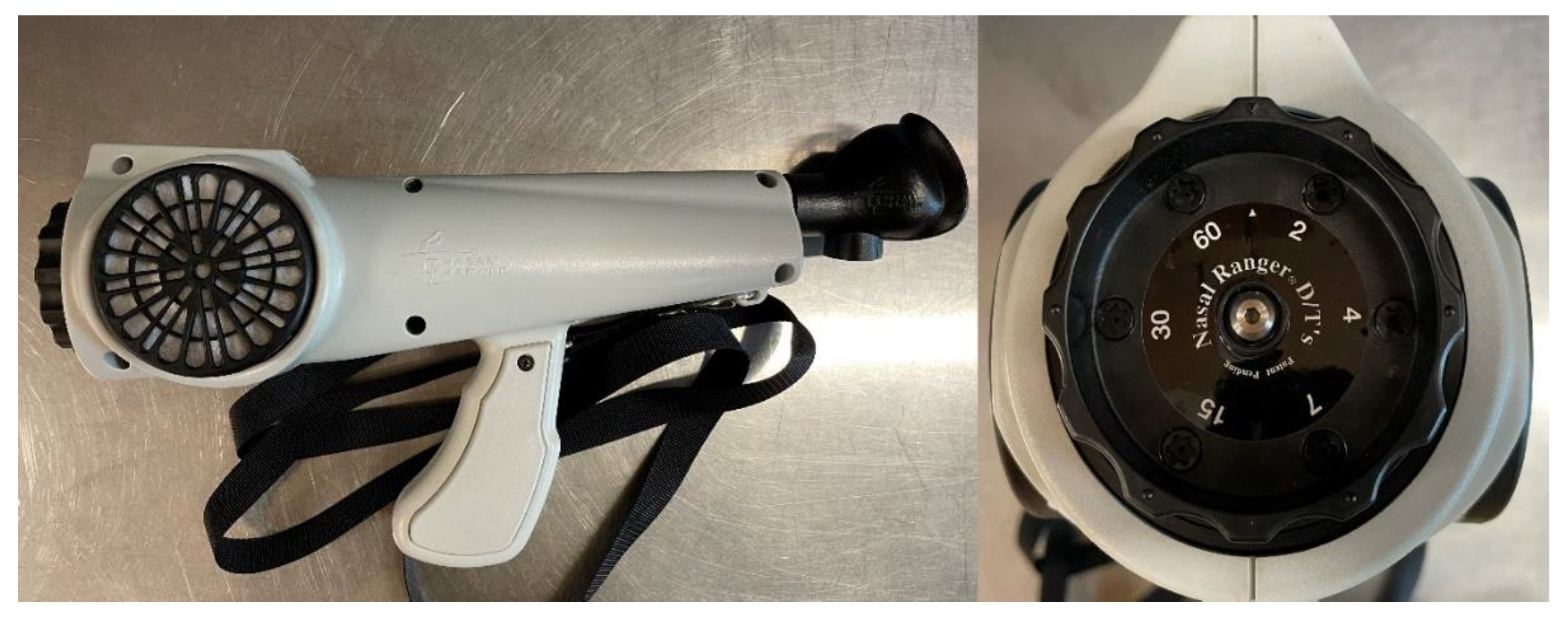
2.2. Odor Concentration Determination by Field Olfactometry

The NasalRanger field olfactometer manufactured by St. Croix Sensory, Inc. (Stillwater, MN, USA) was used in the measurements of odor concentration (Figure 2) [33]. The operating principles of the selected field olfactometer are based on the dilution-to-threshold ratio (D/T). The device mixes odorous air with filtered air to measure the odors in the air. The device has two built-in airflow paths. The first one goes through an orifice on the D/T dial, and the second one goes through a pair of activated-carbon filters located at the sides of the olfactometer. The orifice size on the D/T dial can be changed by rotating the dial, which controls the volume of odorous air that goes to the device.

The dilution to threshold ratio is presented as (Equation (1)) and represents the number of dilutions needed to make odorous air nondetectable.

$$\frac{D}{T}=\frac{Volumeoffilteredair}{Volumeofodorousair}$$

(1)

As shown in Figure 2, the D/T dial has 12 positions, 6 blank positions (only filtered air goes through device), and 6 D/T positions (60, 30, 15, 7, 4, and 2). To preform correct measurement with selected device, the operator has to put the mask of the field olfactometer tightly to the nose and start breathing with the air flow equal to 16–20 L per minute. The inhalation rate is indicated by the LEDs located in the top part of the device. Full instructions for using the olfactometer are available on the manufacturer’s website [33].

By knowing the specific D/T ratio where it was possible to detect the odors and by knowing where it was nondetectable, it is possible the determine to odor concentration expressed as odor unit per cubic meter (ou/m³). The odor concentration calculations in the study were performed with the use of the following formulas (Equations (2)–(5)):

$$Z_{YES}={\left(D/T\right)}_{YES}+1$$

(2)

Z_YES is the dilution ratio at which the odor was detectable during the measurement, and (D/T)_YES is the dilution ratio when the odor was detected for the first time.

$$Z_{NO}={\left(D/T\right)}_{NO}+1$$

(3)

Z_NO is the dilution ratio at which the odor was undetectable during the measurement, and (D/T)_NO is the dilution ratio when the odor was undetected just before the (D/T)_YES.

$$Z_{ITE}=\sqrt{Z_{YES}\ast Z_{NO}}$$

(4)

Z_ITE is assessment of individual threshold, expressed as dilution ratio.

$$Z_{ITE}=C_{od}$$

(5)

C_od is odor concentration, ou/m³.

These formulas are directly based on the principles of the operation of field olfactometer and are in relation to calculations of odor concentration by the means of dynamic olfactometry. They have been widely adopted and used previously by other authors [19,22,23,34,35].

The final odor concentration was presented as Z_ITE due to the fact that the measurements were carried out by a single person. The person taking part in the measurements had previously been tested with the reference substance n-butanol and met the requirements of the EN 13725 standards for measurements with the use of a dynamic olfactometry method. The field olfactometer allowed to obtain a several series of dilutions, D/T, of 60, 30, 15, 7, 4, and 2, which corresponds to odor concentrations equal to 78.49, 43.49, 22.27, 11.31, 6.32, 3.87 ou/m³. In the event of multiple participants that would generate multiple Z_ITE for specific points, the C_od should be presented as a geometric mean. For each point marked out in Figure 1, the final odor concentrations were obtained by using the equations presented above. Results collected with field olfactometry method were used to obtain the spatial distribution of odor concentration with the use of the IDW method.

2.3. Meteorological Data

Weather conditions were monitored throughout the measurement campaign. Meteorological data were measured with a portable handheld weather station Testo 410-2. According to the manufacturer, the temperature measurement range for the device is −10 up to 50 °C with resolution of 0.1 °C, the relative humidity range is from 0% up to 100% (the precision is 2.5% in the range of 5 to 95% RH) with the resolution of 0.1%, the wind speed measuring range is from 0.4 to 20 m/s (the precision is 0.2 m/s + 2% of measured value) with a resolution of 0.1 m/s. Measurements included ambient temperature (°C), relative humidity (%), wind speed (m/s), and wind direction. Meteorological data were collected at points where odor concentrations were measured using a field olfactometer. The results are presented in Section 3.1.

2.4. Inverse Distance Weighted Method

The inverse distance weighted method was used for the interpolation of field olfactometry data. It is a commonly used deterministic method for interpolating environmental data using the following formulas (Equations (6) and (7)) [29,30]:

$$u\left(x,y\right)=\frac{{{\displaystyle \sum }}_{n=1}^N\frac{u_n\left(x_n,y_n\right)}{d_n}}{{{\displaystyle \sum }}_{n=1}^N\frac{1}{d_n}}$$

(6)

$$d_n=\sqrt{{({\left(x-x_n\right)}^2+{\left(y-y_n\right)}^2)}^i}$$

(7)

where N is number of unknown locations, $u\left(x,y\right)$ is values at unknown location, $d_n$ is distance between points, and i is exponential function, usually equal to 2.

The selected method allows to interpolate known values at measured, known locations into unknown locations; therefore, it is possible to obtain continuous surface of selected phenomena. The basic assumption is that points closer to each other are more correlated than those further apart [32]. The values at unknown locations are calculated as weighted average of measurements at known points [29]. Following the basic assumption, the interpolated values are more influenced by closer, known locations, the influence dimmish over distance. Closer proximity of known values gives higher weights [29,32]. The power function (Equation (7)) allows to manipulate the influence of known locations on interpolated values [32,36]. Data interpolation was performed with the use of ArcGIS Pro software and the built-in Geostatistical Wizard tool for every month, where c_od was determined by field olfactometry.

To assess the performance of IDW method, a cross-validation was used. The main reason was to check how the data obtained by the means of selected interpolation method agree with the input data used for interpolation. A leave-one-out method was used for cross-validation, where one point is removed from the dataset, and the value at that location is predicted with the remaining points. Comparison of measured and predicted values allows to obtain parameters that can be used for validation of interpolation [28,37]. The ArcGIS Pro build-in cross-validation tool was used for the task. The ArcGIS Pro (version 3.0.3.) software allows for analysis of two parameters for the IDW method: the mean error ME (Equation (8)) and the root mean square error RMSE (Equation (9)). The power function (Equation (7)) was optimized by the built-in Geostatistical Wizard to obtain the lowest possible cross-validation results.

$$ME=\frac{1}{n}{\displaystyle \sum }_{i=1}^n{I}_i-O_i$$

(8)

$$RMSE=\sqrt{\frac{1}{n}{\displaystyle \sum }_{i=1}^n{(I_i-O_i)}^2}$$

(9)

where $I_i$ is predicted values, $O_i$ is measured values, and n is number of samples.

The ME parameter gives information on the average error of cross-validation, whereas it should be as close to zero, values larger than zero suggest that the model overestimates values, while values smaller than zero suggest underestimation [37]. The RMSE parameter measures the accuracy of the interpolation model. The RMSE should be as small as possible. It gives information on how much predicted values differ from measured values [37].

3. Results and Discussion

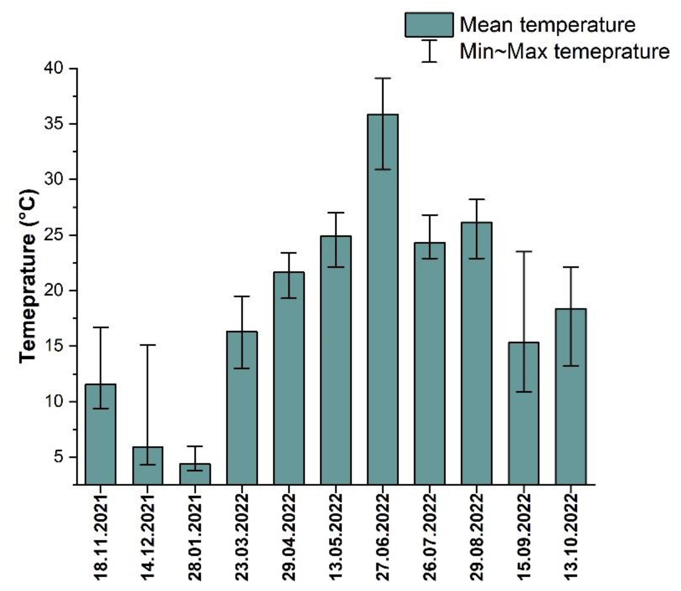
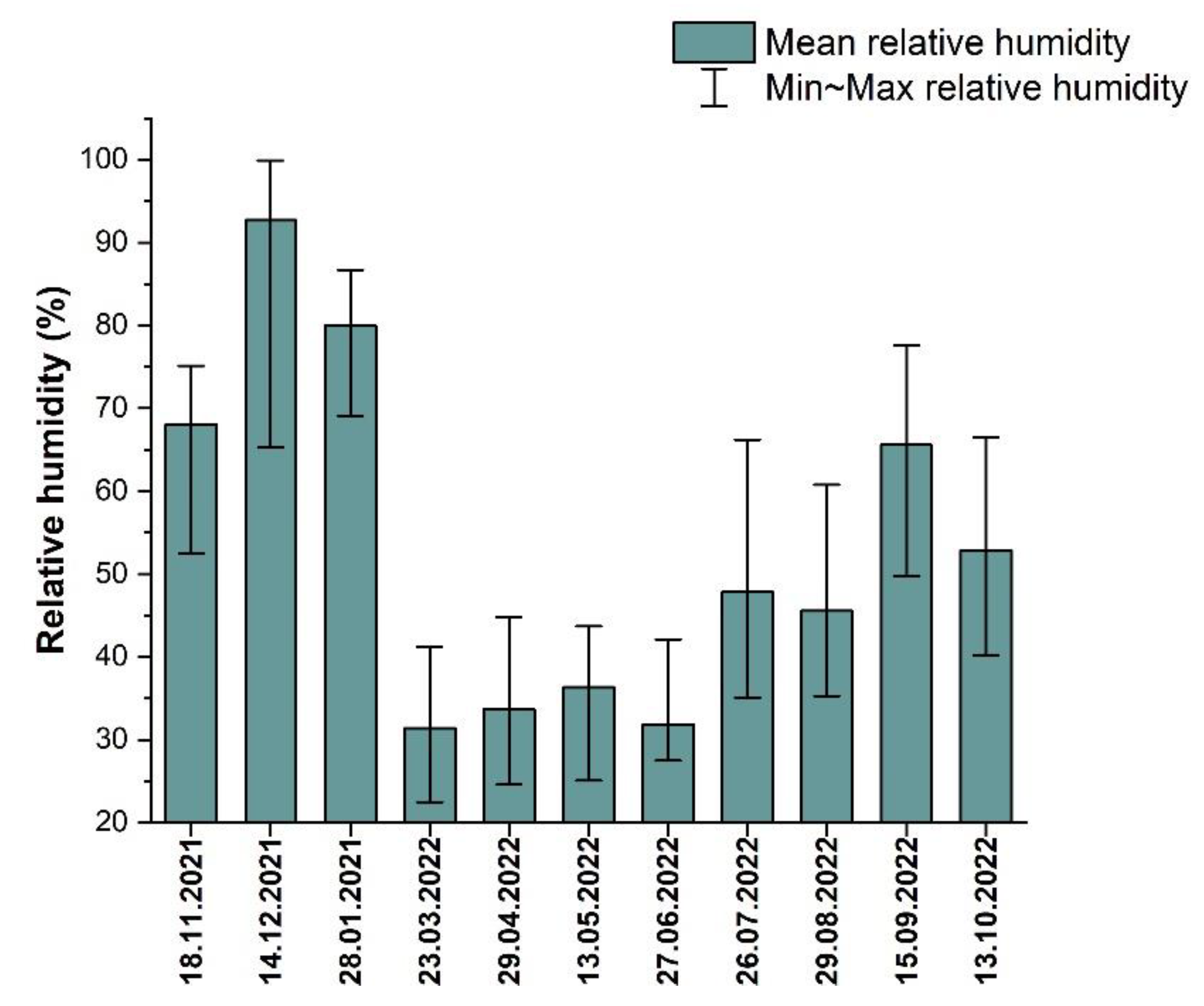
3.1. Meteorological Situation during the Given Measurement Period

Figure 3 shows the mean temperature (°C) along with the minimum and maximum measured value on a given measurement day. The first month measurements were made in was November, where the mean temperature during measurements was 11.56 °C. During the next two months, the mean temperature during the measurements decreased and amounted to 5.92 °C and 4.38 °C for December and January, respectively. During the measurements in November, December, and January, the lowest temperatures in the entire measurement series were recorded. From March to June, the average temperature during the measurements was characterized by an upward trend. It was, respectively: 16.31 °C (March), 21.64 °C (April), 24.89 °C (May), and 35.85 °C (June). In June, the highest temperature was recorded throughout the measurement series. In July, the average temperature during the measurements was 24.28 °C; in August, 26.14 °C; and in September and October, 15.32 °C and 18.37 °C, respectively. Due to the 11-month nature of the measurements (without the month of February), the temperatures measured in a given month show a certain seasonality, i.e., the winter months are characterized by the lowest temperatures, the summer months are characterized by the highest ones, while the spring and fall months are characterized by average values. Figure 4 shows the mean relative humidity (%) along with the maximum and minimum values measured on a given measurement day. As before, in the first measurement month, that is, November, the mean value of relative humidity was 68.07%; in December; this value was 92.72% and was the highest mean value in the entire measurement series. From March to June, a significant decrease in average humidity was observed. It amounted to 31.37% for March, 33.67% for April, 36.33% for May, and 31.89% for June. In June, the lowest average humidity was recorded in the entire measurement series. For July, the average humidity was 47.85%; for August, 45.59%; for September, 65.58%; and 52.91% for October.

3.2. The Results of Field Olfactometry Measurements

The results of field olfactometric measurements for points located in the selected MBT plant (excluding points located inside technological buildings) are presented in

Table 1. Results of field olfactometry measurements for the whole measuring series—excluding technological buildings located inside (for detailed information about specific point location, see Figure 1).

Point Number	18 November 2021	14 December 2021	28 January 2022	23 March 2022	29 April 2022	13 May 2022	27 June 2022	26 July 2022	28 August 2022	15 September 2022	13 October 2022
1	3.87	*	*	3.87	*	*	3.87	11.31	3.87	*	*
2	6.32	*	6.32	3.87	6.32	*	3.87	6.32	6.32	3.87	11.31
4	11.31	*	*	6.32	*	6.32	6.32	6.32	6.32	*	22.27
10	11.31	*	6.32	22.27	11.31	11.31	22.27	43.49	22.27	6.32	11.31
11	22.27	*	3.87	43.49	43.49	22.27	43.49	43.49	43.49	22.27	43.49
12	11.31	*	6.32	22.27	22.27	22.27	43.49	78.49	22.27	22.27	22.27
13	6.32	*	22.27	11.31	6.32	11.31	11.31	22.27	11.31	11.31	11.31
14	43.49	*	*	43.49	22.27	43.49	78.49	78.49	78.49	43.49	78.49
15	43.49	*	*	78.49	78.49	43.49	78.49	78.49	43.49	78.49	78.49
17	11.31	*	*	11.31	6.32	6.32	6.32	6.32	6.32	6.32	3.87
18	78.49	*	3.87	43.49	43.49	11.31	78.49	78.49	78.49	43.49	43.49
25	78.49	*	22.27	78.49	78.49	43.49	43.49	78.49	78.49	43.49	78.49
26	43.49	*	22.27	78.49	43.49	22.27	43.49	43.49	78.49	78.49	78.49
27	22.27	3.87	*	6.32	6.32	11.31	6.32	11.31	11.31	6.32	6.32
28	43.49	6.32	*	43.49	43.49	43.49	78.49	78.49	43.49	78.49	78.49
29	43.49	6.32	*	43.49	78.49	22.27	78.49	43.49	43.49	43.49	78.49
30	22.27	22.27	*	22.27	43.49	43.49	43.49	43.49	43.49	43.49	22.27
31	78.49	43.49	22.27	11.31	11.31	11.31	22.27	22.27	11.31	11.31	22.27
32	3.87	*	*	*	*	*	*	3.87	*	*	*
33	11.31	6.32	*	6.32	6.32	6.32	6.32	6.32	6.32	3.87	6.32
34	11.31	6.32	*	11.31	6.32	6.32	3.87	11.31	3.87	3.87	6.32
35	6.32	11.31	*	6.32	6.32	3.87	3.87	11.31	3.87	11.31	11.31

* below detection threshold.

. The odor concentration for the first measuring point located near the administrative building ranges from 3.87 ou/m³ up to 11.31 ou/m³. The highest value was 11.31 ou/m³, measured during July 2022. During the five measurement months, the odor concentration was below the detection threshold of the field olfactometry method. The second point, a technical area where the facility vehicles are parked and serviced, ranges from 3.87 ou/m³ up to 11.31 ou/m³, where the highest value of 11.31 ou/m³ was measured only once during the last measuring month (October). Only in two months (December 2021 and May 2022) were odor concentrations below the detection threshold. The selective waste storage area was characterized by odor concentrations equal to 22.27 ou/m³. The highest c_od were recorded during October 2022 (22.27 ou/m³) and during November 2021 (11.37 ou/m³). Odor concentrations below the detection threshold were recorded during December 2021, January 2022, April 2022, and September 2022. The rest of the measuring months were characterized by concentrations equal to 6.32 ou/m³. Points number 10, 11, and 12 are located in the vicinity of the landfill site, point number 10 was located near the entrance, and points 11 and 12 were located directly at the landfill site. The odor concentrations for point number 10 range from 6.32 ou/m³ to 43.49 ou/m³. The highest concentration was recorded in July 2022 (43.49 ou/m³), and the lowest measured c_od were determined during January 2022 and September 2022 (6.32 ou/m³). During December 2022, the c_od for was below the detection threshold. The same situation can be observed for points number 11, 12, 13, 14, 15, 17, 18, 25, 26, and 32. C_od at point number 11 ranges from 3.87 ou/m³ to 43.49 ou/m³. During most of the measuring months, the odor concentration was equal to or greater than 22.27 ou/m³. During January 2022, the odor concentration was 6.32 ou/m³. A similar situation can be observed in the case of point 12. It ranges from 6.32 ou/m³ up to 78.49 ou/m³. The lowest value was observed during January 2022, and the highest value was observed during July 2022. The rest of the measuring months were in the range of 22.27 ou/m³ to 43.49 ou/m³. The bulky waste storage area (point number 13) was characterized by odor concentrations ranging from 6.32 ou/m³ to 22.27 ou/m³. The highest c_od were observed during January 2022 and August 2022. The lowest was during November 2021 and April 2022 (6.32 ou/m³), while the rest of the measuring months were at the level of 11.31 ou/m³. Points 14, 15, 28, and 29 are located in the vicinity of the aerobic stabilization area. As can be observed, the overall trend shows that the c_od for those points is relatively high, with a few exceptions. Most of the time, the value of odor concentrations ranges from 43.49 ou/m³ up to 78.49 ou/m³. The values of 22.27 were recorded during April 2022 (point 14) and May 2022 (point 29). December 2021 and January 2022 are the months where the c_od is much different from in the rest of the measuring series. As mentioned above, c_od at points number 14, 15, and 28 during December 2022 was below the detection threshold. C_od at points 28 and 29 is significantly lower (6.32 ou/m³) than in the rest of the months. The c_od during January 2022 was below the detection threshold for the whole aerobic stabilization area. The points located near the green waste storage area (18, 26) show trends similar to the aerobic stabilization area, which is in the direct vicinity. During December 2021, the c_od was below the detection threshold for both points. January 2022 is characterized by the lowest value of c_od at point number 18, and the second lowest value was measured in May 2022 (11.31 ou/m³), while during the rest of the measuring series, c_od ranges from 43.49 up to 78.49 ou/m³. In the case of point 26, the lowest values were observed during January 2022 and May 2022 (22.27 ou/m³), while during the rest of the measuring series, the odor concentrations were in the range of 43.49 ou/m³ up to 78.40 ou/m³. Measuring point number 25 was located between the aerobic stabilization chambers and the green waste storage area. The trend is similar. The concentrations range from 22.27 up to 78.49 ou/m³. Two measuring points were located in the middle of two biofilters: 17—biofilter for anaerobic processes and 27—biofilter for aerobic processes. Although in close proximity to other odor sources, i.e., aerobic stabilization area and green waste storage area, the c_od measured during the whole measuring series is relatively low compared to the other points in the close vicinity. Four of the measurement points were located near the leachate tanks. Point 31 was located near a tank for biological processes, and points 33, 33, and 34 were near two tanks for landfill leachates. A biological leachate tank is characterized by the highest concentrations of all points located near leachate all tanks. The highest concentration was measured during November 2021 and was equal to 78.49 ou/m³. The second highest concentration was recorded during December 2021, 43.49 ou/m³. Since then, the c_od has ranged from 11.31 ou/m³ to 22.27 ou/m³. This is the only point where it was possible to obtain odor concentrations for all measuring months. When it comes to points number 33, 34, and 35, odor concentrations range from 3.87 ou/m³ to 11.31 ou/m³, with the except for February 22, where the c_od was below the detection threshold. Point 33 was located in the corner of the MBT plant, near the fence, separated from the proximity of odor sources. In most cases, the odor concentrations were below the detection threshold, with the exception of November 2021 and July 2022, and it was equal to 3.87 ou/m³.

The results of the odor concentration measurements carried out inside technological buildings at a selected MBT plant are presented in

Table 2. Results of odor measurements carried out inside technological buildings located at selected MBT plant (for detailed information about specific point location, see Figure 1).

Point Number	18 November 2021	14 December 2021	28 January 2022	23 March 2022	29 April 2022	13 May 2022	27 June 2022	26 July 2022	28 August 2022	15 September 2022	13 October 2022
3	22.27	**	11.31	11.31	11.31	11.31	11.31	11.31	11.31	11.31	78.49
5	6.32	**	**	11.31	6.32	3.87	3.87	6.32	6.32	3.87	43.49
6	3.87	***	***	3.87	***	***	***	***	3.87	***	6.32
7	3.87	***	***	3.87	***	***	***	***	3.87	***	3.87
8	6.32	***	***	11.31	***	***	***	***	6.32	***	6.32
9	22.27	**	22.27	22.27	43.49	43.49	43.49	78.49	43.49	43.49	43.49
16	43.49	**	43.49	43.49	78.49	78.49	78.49	43.49	43.49	43.49	78.49
19	43.49	*	*	78.49	*	*	*	*	*	*	78.49
20	78.49	*	*	78.49	*	*	*	*	78.49	*	78.49
21	*	*	*	*	*	*	*	*	*	*	78.49
22	78.49	*	*	*	78.49	*	*	*	78.49	78.49	78.49
23	*	*	*	*	78.49	*	*	*	*	78.49	78.49
24	*	*	*	*	*	*	*	*	*	*	78.49

* bioreactors were closed, and measurements were not possible. ** below the detection threshold. *** the sorting line was stopped/not operational during the measurements.

. During the first measuring month (18 November 2021), the lowest concentrations were measured inside the sorting hall (points 5–8). The lowest concentration inside the sorting hall was recorded in sorting cabins 1 and 2 and was equal to 3.87 ou/m³. Points located in the middle of the sorting hall and at the beginning of the sorting line (points no. 5 and 8) valued at 6.32 ou/m³. Concentration in the waste reception hall valued at 22.27 ou/m³, similar to RDF preparation and storage building. The concentrations in the technological building of the anaerobic processes and within Bioreactor 1 were equal to 43.49 ou/m³. The highest concentrations were recorded inside bioreactors 2 and 4. The rest of the bioreactors were closed during the measurement day, and, therefore, measurements inside them were not possible. During the second month of the measurement series (14 December 2021), it was not possible to determine the odor concentrations at selected measurement points. All of the bioreactors were closed; therefore, it was not possible to determine the c_od. During the measuring series carried out in January 2022, it was possible to determine c_od inside the technological building of anaerobic processes (43.49 ou/m³), inside the waste reception hall (22.27 ou/m³), and the RDF preparation and storage building (11.31 ou/m³) During the rest of the measuring series, the results were gathered without problems indicated before, and the c_od was determined as in the case of the first month. The lowest concentrations were observed inside the sorting hall. The lowest concentrations were observed inside sorting cabins 1 and were 2 and valued at 3.87 ou/m³, similar to what was in November 2021. Concentrations in the middle of the sorting hall and at the beginning of the sorting line were slightly higher and accounted for 11.31 ou/m³. The odor concentration in the RDF preparation and storage building was valued at 11.31 and was lower than in the case of November 2021 and was stable until October 2022, when the concentration inside RDF preparation and storage building valued to 78.49 ou/m³. From March 2022 until July 2022, the sorting line was stopped during the measurements, so it was not possible to determine the odor concentrations inside the sorting cabins. Odor concentration in July for sorting cabin 1 and 2 was the same as in the case of March and November. September was another month when the sorting line was stopped during measurement day. During October (13.10.2022), the concentration inside sorting cabin 1 was 6.32 ou/m³ and was higher than in the previous months. Sorting cabin 2 valued at 3.87 ou/m³. The concentration in the center of the sorting line ranged from 3.87 ou/m³ to 6.32 ou/m³ from April to July, where the concentration at the beginning of the sorting line was not determined due to the fact that the line was stopped. October (13.10.2022) showed a significant increase in the odor concentration in the middle of the sorting hall, which valued to 43.49 ou/m³, where the beginning of the sorting line was characterized by an odor concentration equal to 6.32 ou/m³. The waste reception hall during March 2022 was characterized by an odor concentration equal to 22.27 ou/m³. From then until the end of the measurements, the measured concentration in the waste reception hall was 43.49 ou/m³, except for July 2022, where the concentration was 78.49 ou/m³. The concentration inside the technological building of anaerobic processes was in the range of 43.49 ou/m³ to 78.49 ou/m³ (period from March to October). The concentrations inside bioreactors were equal to 78.49 ou/m³ for almost the entire measuring series, except for Bioreactor 1 during November 2021, where the c_od was equal to 43.49 ou/m³.

The obtained results of c_od measurements allowed for the identification of areas and technological processes affected by the highest odor concentrations, i.e., aerobic stabilization area, green waste storage area, bioreactors or waste reception hall. It is clearly visible that areas where high accumulation of organic waste takes place are characterized by highest odor concentration. Hence, it is possible to conclude that those places are responsible for highest odor emissions.

Limited recent literature is available considering studies of odor concentrations measurements by the means of field olfactometry at mechanical biological waste management plants. Examples can be found in [19,20,34,38,39,40]. Authors of [19] carried out research at 6 different MBT waste treatment plants equipped with biogas producing installations with the use of fermentation method. The odor concentrations were measured at similar measurement points to the points in the study being the subject of this article, i.e., waste storage, mechanical part of selected plants, fermentation preparation (inside buildings), digestate dewatering, oxygen stabilization areas, or biofilters areas. When analyzing the results, c_od for waste storage ranged from 4 ou/m³ up to 106 ou/m³ [19,34], which was similar to results obtained in point 9 (c_od ranges from 22.27 ou/m³ up to 78.49 ou/m³). It is worth noting that [19,34] used a filed olfactometer with two different D/T dials; the second one allowed for dilution of 60, 100, 200, 300, and 500, which resulted in higher c_od range. Therefore, when using D/T dials with lower dilution ranges, it is possible to miss the right odor concentration because the measuring methodology does not allow for exceeding the D/T of 60 with lower dilution range dial. This creates the possibility of underestimating odor concentrations. The methodology is limited to determination of 78.49 ou/m³, while the real c_od can be higher. Therefore, when operating the field olfactometers, the high dilution D/T dial should be also used in evaluations. The odor concentrations at mechanical parts of studied objects [19,34] ranges from 4 up to 11 ou/m³. Similar to points 6, 7, and 8 (3.87 ou/m³ up to 11.31 ou/m³). The highest difference can be observed when it comes to aerobic stabilization. Authors of [19,34] found c_od at levels from 4 ou/m³ up to 22 ou/m³. It is significantly different from points 14, 15, 28, and 29, where c_od valued at 43.49 ou/m³ up to 78.49 ou/m³. Authors of [20] found c_od at waste storage and mixed waste storage points at range of 5 up to 12 ou/m³ (lower than point 9), c_od at selectively collected waste measuring points valued for around 7 ou/m³, quite similar to point 4. The results of odor concentrations for the surface of biofilters are in range of 2 ou/m³ up to 78 ou/m³ [19,20,34,40], while c_od points number 17 and 27 is in range of 3.87 ou/m³ up to 22.27 ou/m³. The higher ranges of c_od at biofilters could be associated with improper working conditions. The operating conditions are one of the factors that can affect emission of odors, therefore affecting the measured odor concentrations, and technological operations and type of processed waste [19,34]. Another example could be found at [39]. Authors investigated leachate tanks at two different MBT plants. They used different kinds of portable olfactometers that allowed for higher range of c_od determination. The c_od ranges from 22 ou/m³ up to 6390 ou/m³. Those values are much higher than those obtained for points 31, 33, 34, and 35. In [19], the highest odor concentration was obtained for digestate dewatering (from 8 ou/m³ up to 448 ou/m³); in [34], the highest was waste storage (106 ou/m³); and in [20], it was oxygen stabilization area with highest c_od. The available literature shows high variability in odor concentration despite some of similarities. Thus, the question is: is it possible to get very similar results for different MBT plants? The answer is no. As shown in the literature [24,41], the composition of waste is constantly changing and can be different at levels of communities, cities, or regions. Therefore, the waste processed in MBT plants located in two different regions can be different in terms, for example, of amount of organic matter, so the emission of odors associated with processing organic waste can also be different. The second important fact is that despite the similarities in technology, individual MBT facilities may differ in terms of certain processes, which may also cause differences in odor emissions and affect the odor concentrations.

3.3. Statistical Relationship of Collected Data

To investigate the possible relationship between c_od and meteorological parameters, such as temperature and humidity, statistical tests were performed. At first, the Shapiro–Wilk (SW) test was performed to assess the distribution of data [42]. The results obtained from normality tests were used to choose the appropriate method of data correlation analysis. Normality tests were performed for c_od, temperature, and humidity for each measuring month. The tests covered the whole data set, including both points measured outside and inside. The Shapiro–Wilk test examines how closely the collected data fit to a normal distribution [42]. The hypothesis of normality for the SW test is rejected when the p-value is less than or equal 0.05. The calculations were performed with the use of Origin software.

As

Table 3. Results of the Shapiro–Wilk tests.

	Odor Concentration			Temperature			Humidity
Date	Statistic	p-Value	Decision at Level (5%)	Statistic	p-Value	Decision at Level (5%)	Statistic	p-Value	Decision at Level (5%)
18 November 2021	0.81065	<0.05	reject normality	0.81952	<0.05	reject normality	0.88308	<0.05	reject normality
14 December 2021	0.69823	<0.05	reject normality	0.59594	<0.05	reject normality	0.71975	<0.05	reject normality
28 January 2022	0.83126	<0.05	reject normality	0.78834	<0.05	reject normality	0.92713	>0.05	cannot reject normality
23 March 2022	0.79742	<0.05	reject normality	0.94903	>0.05	cannot reject normality	0.94190	>0.05	cannot reject normality
29 April 2022	0.79742	<0.05	reject normality	0.88698	<0.05	reject normality	0.96850	>0.05	cannot reject normality
13 May 2022	0.81886	<0.05	reject normality	0.94852	>0.05	cannot reject normality	0.96741	>0.05	cannot reject normality
27 June 2022	0.80947	<0.05	reject normality	0.87822	<0.05	reject normality	0.85298	<0.05	reject normality
26 July 2022	0.81105	<0.05	reject normality	0.95002	>0.05	cannot reject normality	0.94166	>0.05	cannot reject normality
28 August 2022	0.79580	<0.05	reject normality	0.94524	>0.05	cannot reject normality	0.94997	>0.05	cannot reject normality
15 September 2022	0.82769	<0.05	reject normality	0.87924	<0.05	reject normality	0.96101	>0.05	cannot reject normality
13 October 2022	0.77401	<0.05	reject normality	0.94977	>0.05	cannot reject normality	0.98543	>0.05	cannot reject normality

shows, the data regarding odor concentrations are not normally distributed for every single measuring month. When it comes to temperature and humidity, the distribution of data is mixed. Based on the results of the Shapiro–Wilk tests, Spearman’s (r_s) correlation was used to find the correlation between data [43]. The r_s test measures the monotonic relationship between the data [44].

Analyzing the relationship between c_od and temperature, it can be observed that in most cases, there is no monotonic correlation, or the monotonic correlation is weak between the odor concentration and temperature. The highest monotonic correlation can be found during May 2022, where the Spearman’s r_s was valued at 0.71479, which could be interpreted as a strong correlation. The second highest value of r_s is observed for July 2022 (0.31703). The rest of the months are characterized by r_s in the range of −0.1 up to 0.2. A similar trend can be observed for the c_od—humidity relationship. Although the overall trend has shown that the correlation is weak, the r_s values for the c_od—humidity relationship is, in general, higher than in case of c_od—temperature. The highest values of r_s were calculated for July 2022 (0.63) and August 2022 (0.47584), while the rest of the measurement months were characterized by r_s in the range of −0.1 to 0.3. The results show that in most cases, measured odor concentrations were not influenced by meteorological parameters, such as temperature and humidity. The possible explanation for this is that the measurements were taken under relatively short amount of time (4–5 min per measuring points). Such approach could affect the possible correlation between data as no averaging overtime of such parameters was performed. However, averaging measurements over higher time range for every measuring point would be in the opposition to the scope of field olfactometry, which is used for in situ measurements relatively short time scale. Nevertheless, it opens a way for possible research regarding a right approach for determining the relationship between field olfactometer measurements and meteorological parameters. If comparing average odor concentration (for each measuring month, including both inside and outside measuring points) with average temperature and humidity, it is unlikely to find any significant relationship. The average c_od for each measuring month is, respectively: 28.85 (November 2021), 13.28 (December 2021), 16.07 (January 2022), 28.75 (March 2022), 34.44 (April 2022), 23.02 (May 2022), 33.75 (June 2022), 36.42 (July 2022), 30.75 (August 2022), 32.84 (September 2022), and 43.83 (October 2022) ou/m³. The highest average c_od was measured during October 2022 at temperature 18.37 °C, while at the highest measured average temperature 35.87 °C (June 2022), the c_od was 33.75 ou/m3.

The results shown in

Table 4. Correlation between odor concentration and meteorological parameters, temperature, and humidity.

	18 November 2021	14 December 2021	28 January 2022	23 March 2022	29 April 2022	13 May 2022	27 June 2022	26 July 2022	28 August 2022	15 September 2022	13 October 2022
	Spearman’s Correlation rs
cod–temperature	−0.10666	−0.09628	−0.15873	0.20211	0.06973	0.71479	−0.01299	0.31703	0.23345	0.21114	0.08681
cod–humidity	0.20527	0.31262	0.28485	0.14397	−0.10124	0.2041	0.15626	0.63653	0.47584	0.14597	0.29144

are calculated for every measuring month; when considering the whole dataset (one single test per relationship), the c_od-temperature r_s valued at 0.0967, while c_od-humidity valued at 0.02264, which confirms that there is no monotonic correlation between analyzed parameters. When considering the available literature, different results can be found regarding relationship between odor concentrations and meteorological parameters such as temperature and relative humidity [45]. For example, authors of [34] concluded that significant relations were observed during their research between odor concentrations (measured with FO method) and temperature. Some dependencies were also observed in the concentration–humidity relationship. However, the same paper [34] shows that the Spearman correlation coefficient valued for 0.306 for c_od-temperature dependency, which could not be considered as a strong correlation. Some of the recent available literatures focused on showing the relationship between temperature, relative humidity, and the concentration of odorants, such as VOCs, H₂S, or NH₃ [34,39,45]. Those studies show existing correlations and dependencies between c_od and odorants and the relationships between odorants and meteorological parameters such as temperature and humidity.

In addition, from the perspective of whole data set, two months are interesting. These months are December 2021 and January 2022. As mentioned before, during these months, it was not possible to determine c_od at almost every point. The possible explanation for the situation is in meteorological data. These two months are characterized by the lowest temperatures and the highest humidity levels during the entire measurement series. It is worth mentioning that the person who was operating the field olfactometer during the measuring series reported that the conditions for those two months were challenging for operating the field olfactometer. The high humidity could also affect the filed olfactometer itself by interfering with the carbon filters built into the device.

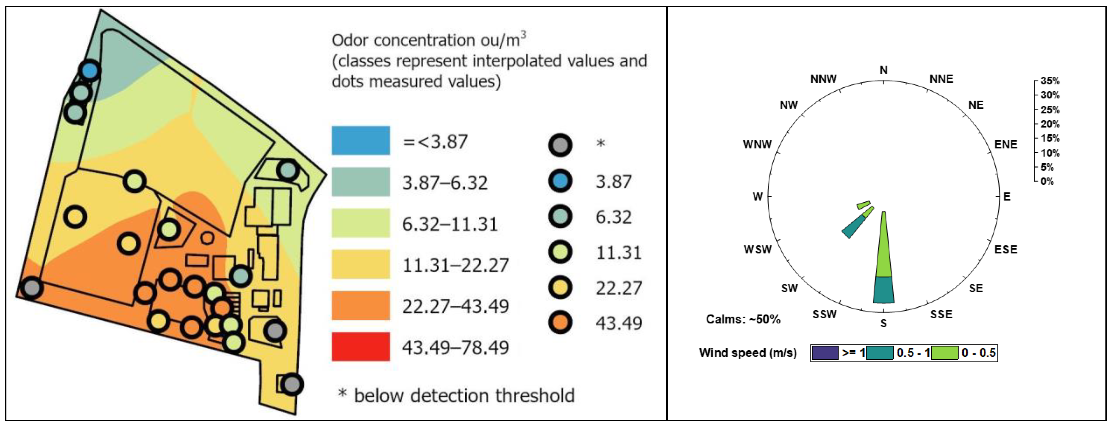
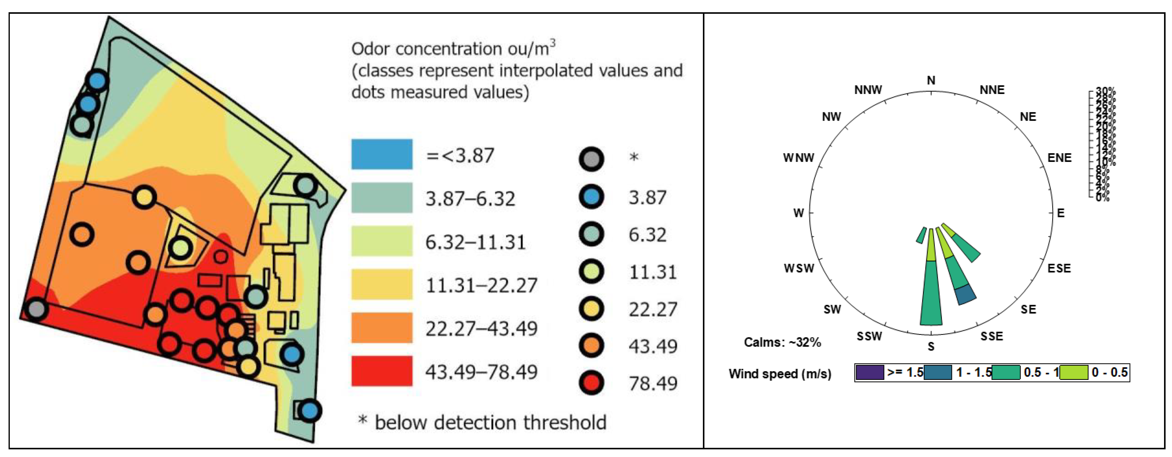
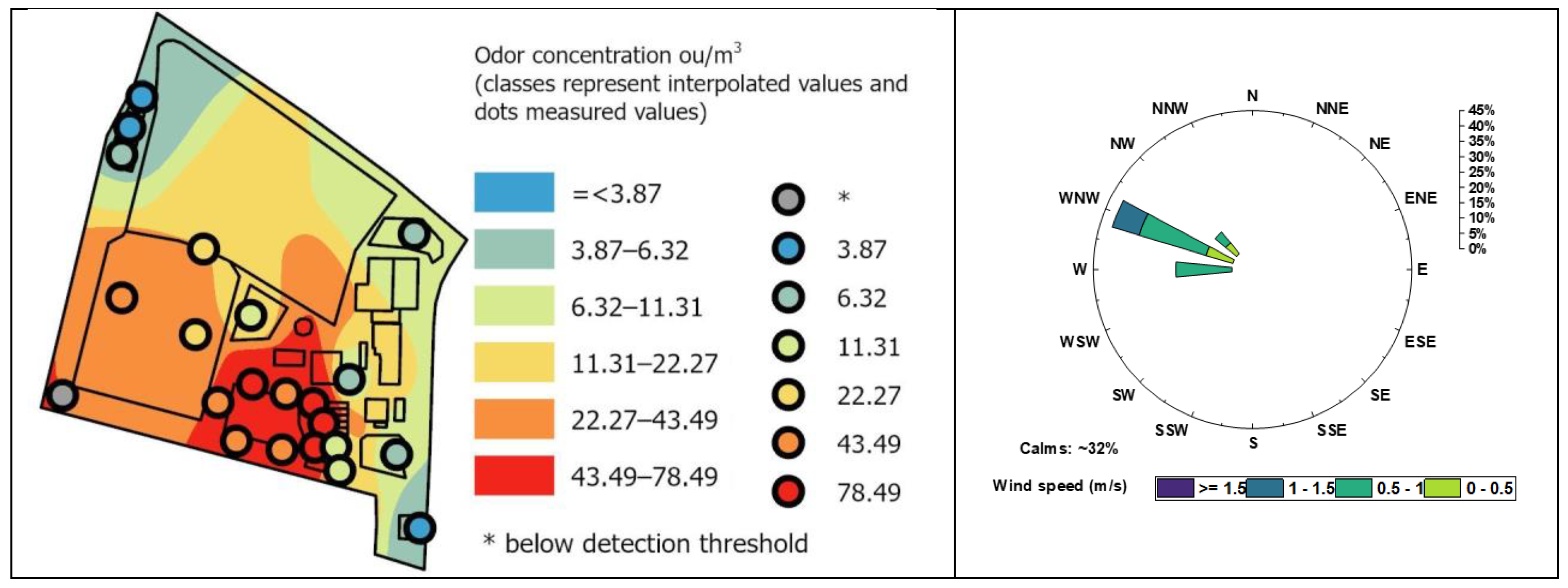
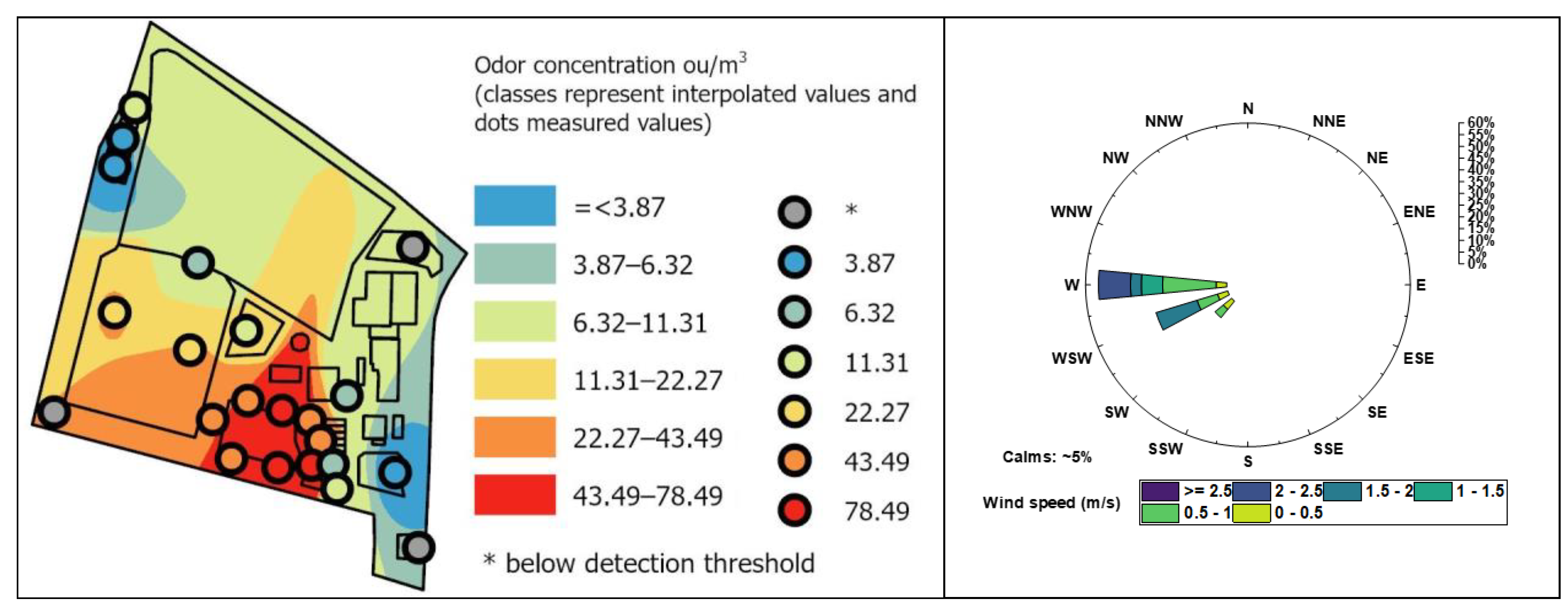
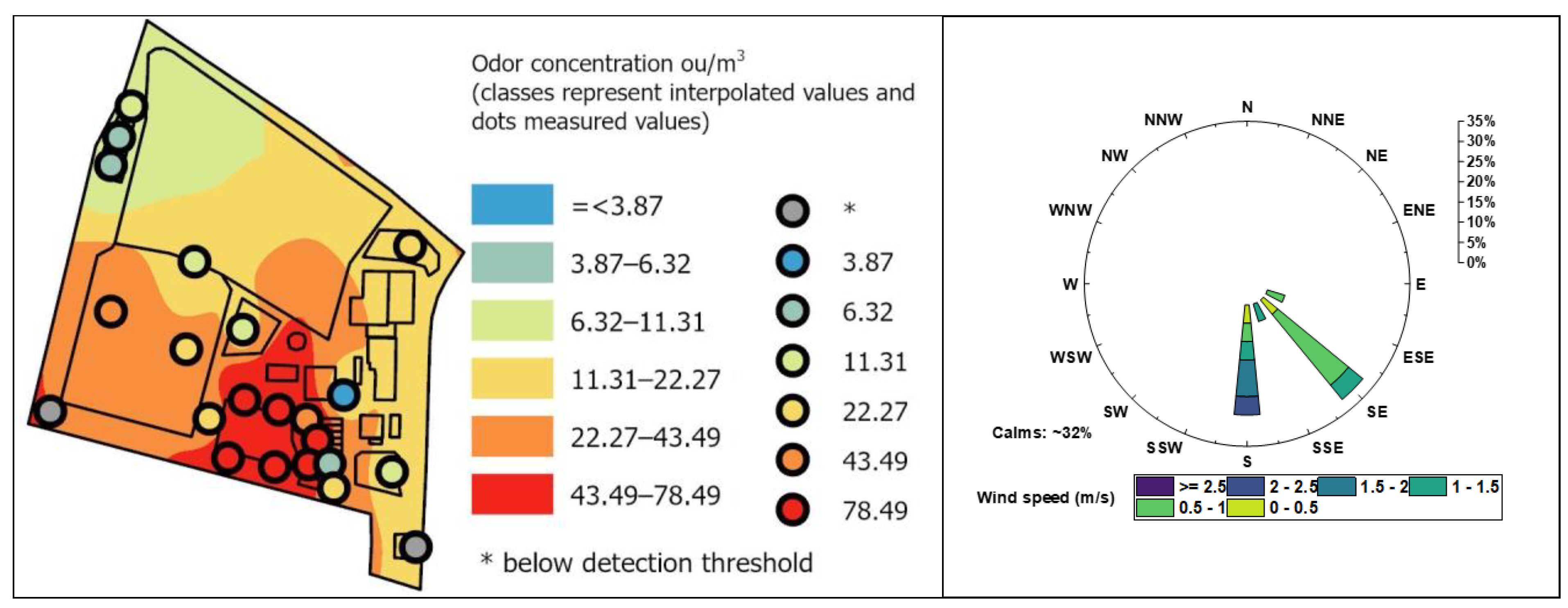
3.4. Spatial Distribution of Odor Concentration and Cross-Validation

Figure 5, Figure 6, Figure 7, Figure 8, Figure 9, Figure 10, Figure 11, Figure 12, Figure 13, Figure 14 and Figure 15 show the spatial distribution of the odor concentration obtained with the IDW method for each measuring month. The interpolated values were classified into 6 classes that correspond to the measuring range of used field olfactometer. For each figure, measured values are also presented (see Figure 1. for detailed information about point numbers and location). Each figure is also coupled with the wind rose plotted from the wind data collected during the measuring day. For Figure 6 and Figure 7 (14.12.2021 and 28.01.2022, respectively), the interpolation was not performed due to the small number of points where c_od was measured. Additionally, the cross-validation results for each spatial distribution obtained for each measuring month are presented in

Table 5. Cross-validation results for the IDW method.

	18 November 2021	14 December 2021	28 January 2022	23 March 2022	29 April 2022	13 May 2022	27 June 2022	26 July 2022	28 August 2022	15 September 2022	13 October 2022
Count	22	-	-	21	19	19	21	22	21	19	20
Mean Error	4.99	-	-	3.61	2.70	1.06	1.69	4.71	5.01	2.16	1.92
Root Mean Square Error	21.88	-	-	21.02	24.03	13.24	20.70	23.06	22.09	17.49	26.70

(with exception for 14 December 2021 and 28 January 2022).

Analyzing the obtained c_od distributions, together with cross-validation results, the following can be observed:

• The cross-validation results show that ME (Equation (8)) in every case is higher than zero, which means that the interpolation formula tends to overestimate the predicted values.
• The RMSE parameter (Equation (9)) is relatively high; the lowest value of RMSE was obtained for the data measured in May 2022 and is equal to 13.24, which means that the predicted values differ on average of 13.24 ou/m³ from the measured values, the highest RMSE was calculated for October 2022; in that case, predicted values differs on average 26.70 ou/m³.
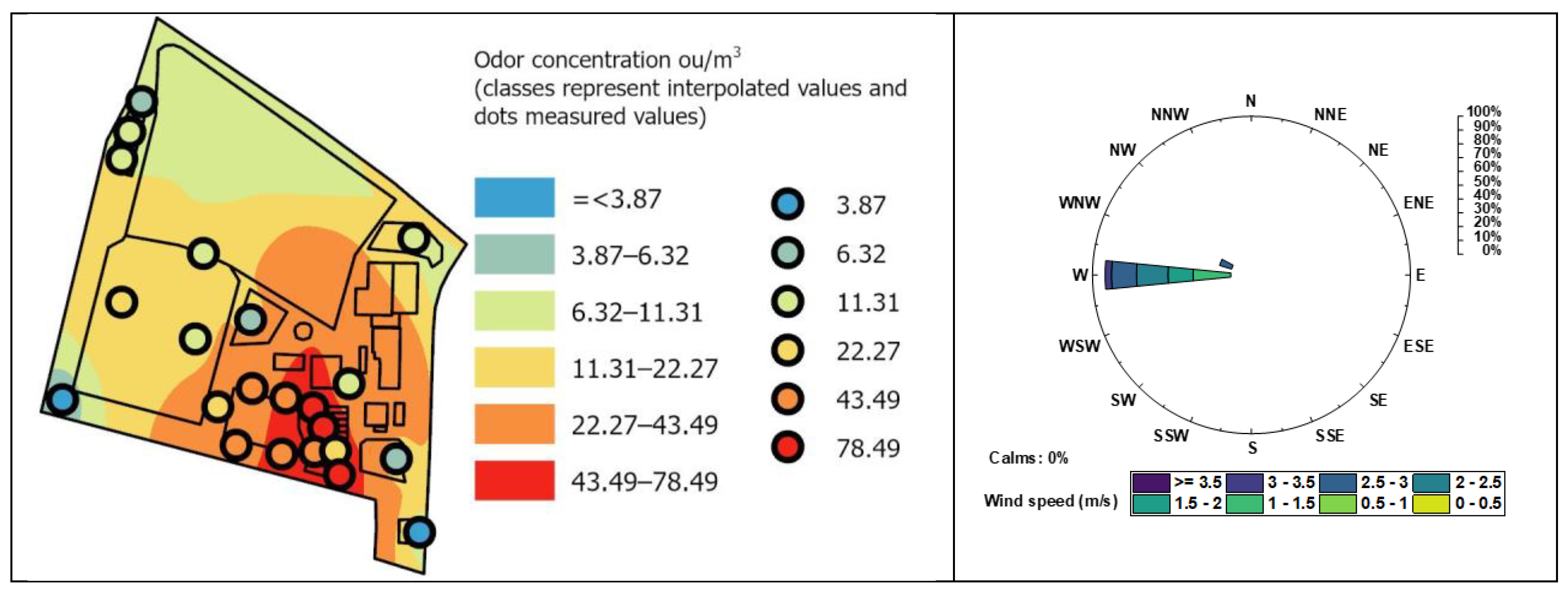
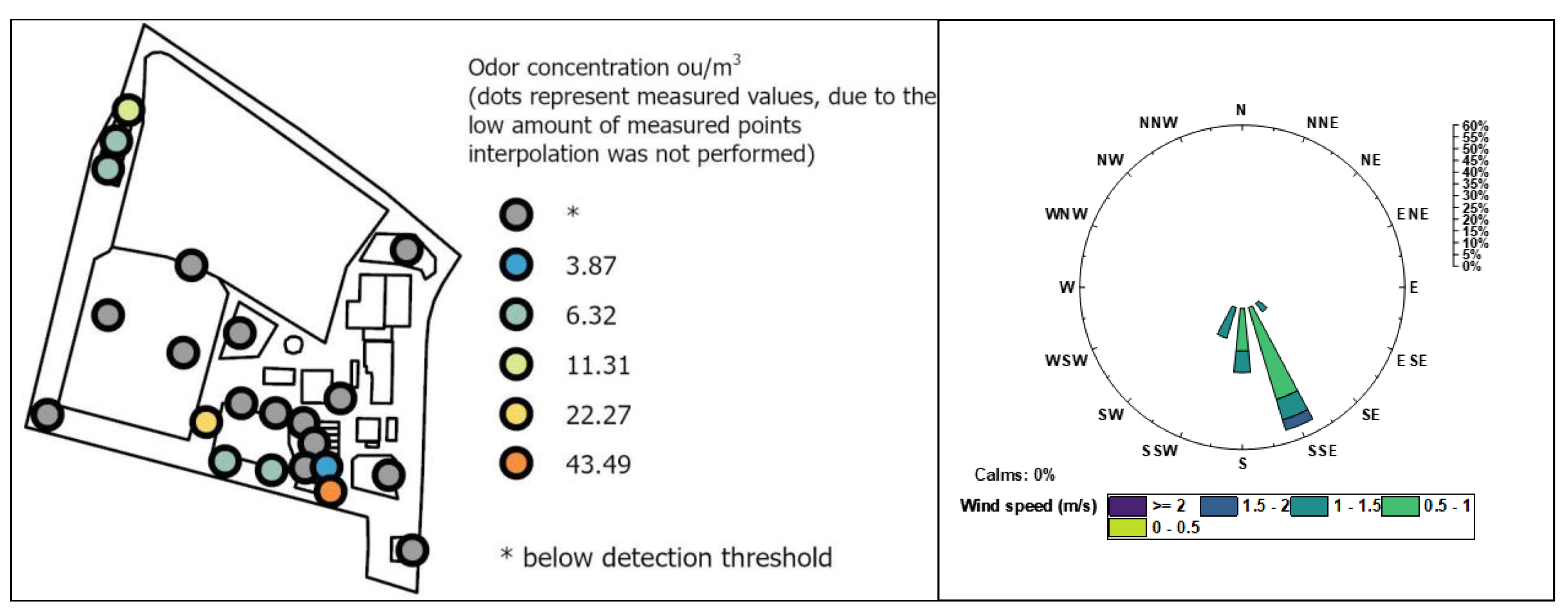
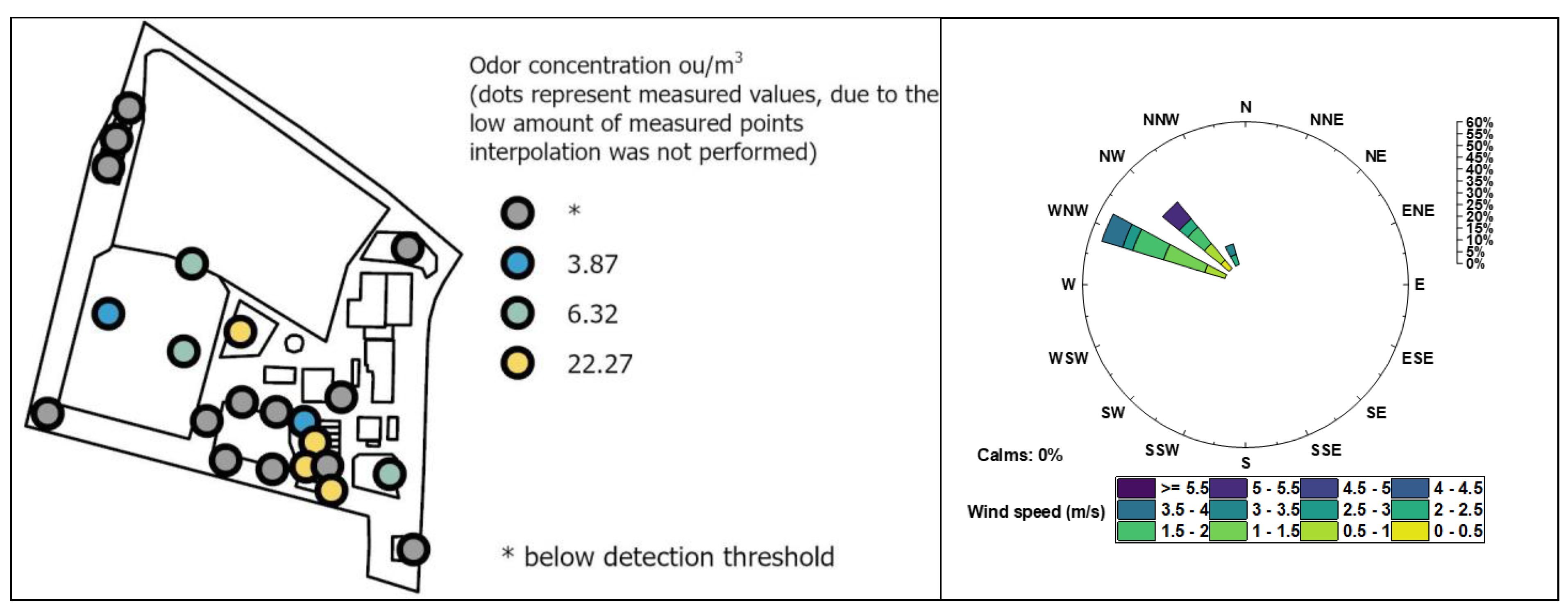
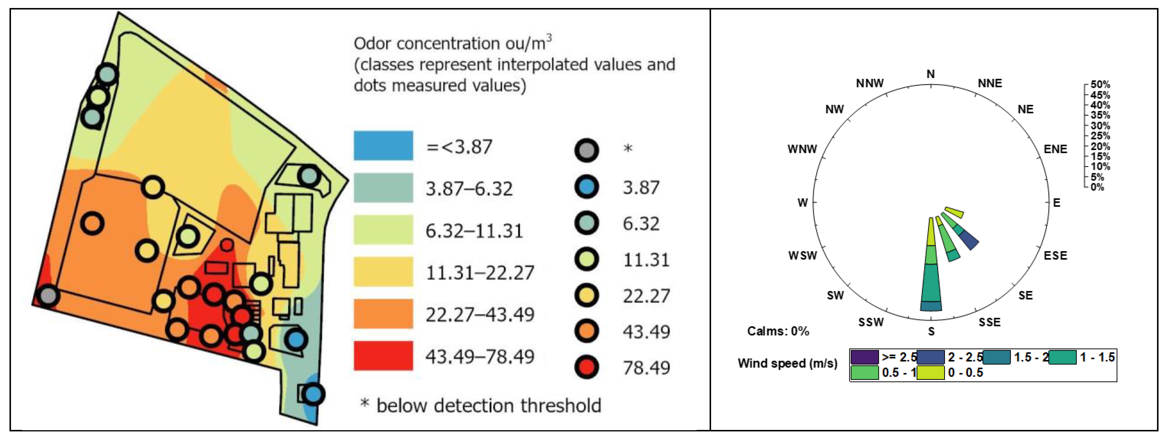
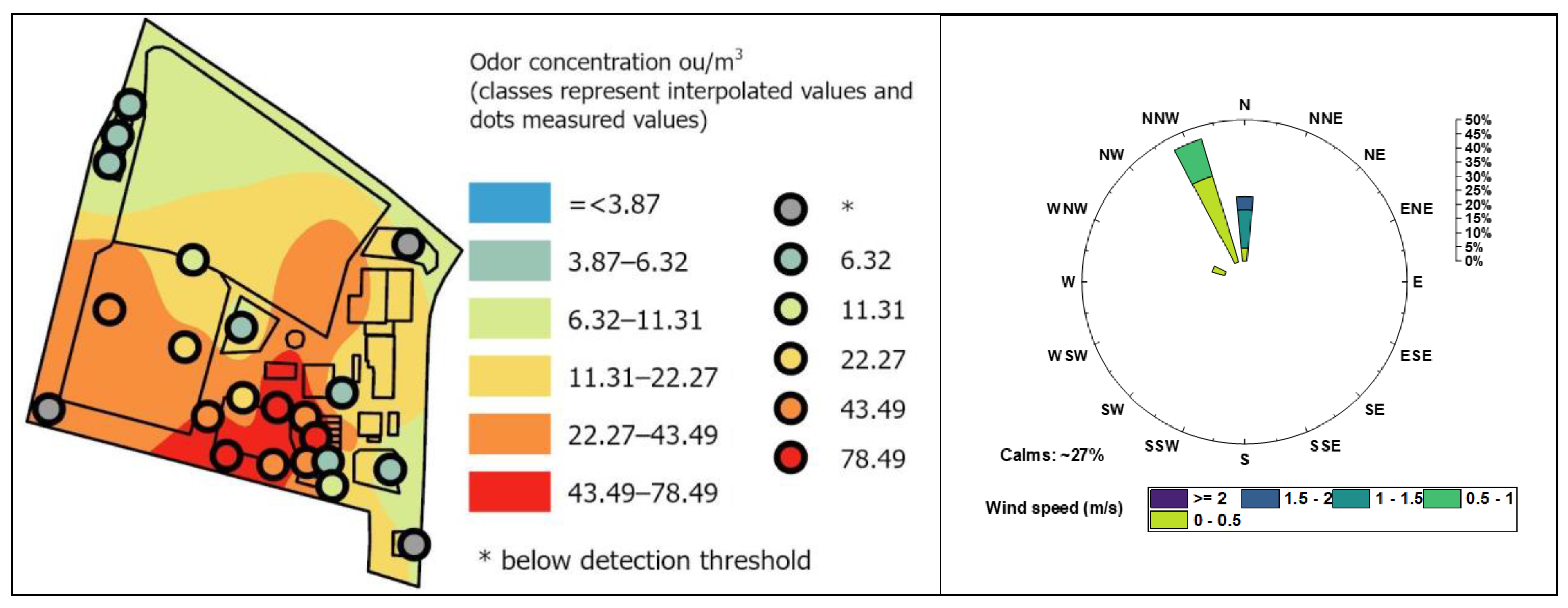
• The analysis of spatial distribution (Figure 5, Figure 6, Figure 7, Figure 8, Figure 9, Figure 10, Figure 11, Figure 12, Figure 13, Figure 14 and Figure 15) confirms the results of cross-validation. In every case, some of the interpolated values differ from measured values and are higher than measured values. The largest difference could be seen when considering lower values. For example, as can be seen in Figure 5, the measured values at the corners of the MBT plant (southeast corner, point 1, administration building and southwest corner, point 32, site boundary) are 3.87 ou/m³, while predicted values obtained by the IDW method are in the range of 3.87 to 6.32 ou/m³. A similar situation can be seen in the middle of the facility (point 13 located in the bulky waste processing and storage area), measured value for that point is 6.32 ou/m³, and the surrounding class is in the range of 6.32 ou/m³ to 11.31 ou/m³ and changes rapidly to the range of 11.31 to 22.27 ou/m³. Such a pattern where lowest measured values do not match with the predicted values is in common for almost every spatial distribution. However, in case of Figure 8 and Figure 14. some of the lower values match exactly with the class—Figure 8, point 1; and Figure 15, points 2, 33, and 34.
• The biggest concern when it comes to results of interpolations are the months when some of the odor concentration at measuring points were below detection threshold. This can be seen in Figure 8, Figure 9, Figure 10, Figure 11, Figure 12, Figure 13, Figure 14 and Figure 15. For example, in Figure 8, at point 32 (left lower corner of the facility), the c_od was below the detection threshold, and the predicted value for that point falls into the highest possible class ranges from 43.49 up to 78.49 ou/m³, which overestimate spatial distribution around that point for almost the whole possible range of odor concentrations.
• Despite the problems mentioned above, it is possible to distinguish areas characterized by higher odor concentrations from areas characterized by lower odor concentrations. For every spatial distribution obtained for given measuring month, it is clearly visible that points scattered around aerobic stabilization area and green storage area are characterized by the highest c_od; therefore, it is possible to find areas that could be possibly influenced by odor emissions or could be the odor emitters by itself. It indicates that the spatial interpolation method could possibly be used for identification of areas influenced by odors and the identification of odor sources.
• Comparing the results of odor concentration measurements by the mean of field olfactometry and the spatial distribution of odor concentrations with the wind rose for each measurement month, it is mostly unlikely to find relationship between odor distribution and wind conditions. The presented wind roses were plotted from the wind data obtained for each measuring point; the data was collected during 3–4 h period. The plotted wind roses do not represent the whole meteorological conditions as it could be influenced by local factors. Therefore, the more accurate research should be provided in the future.

IDW method, despite being easy to compute, fast, and simple in terms of a mathematical relationship, has a number of disadvantages [30,31]. The inverse distance weighted method is sensitive to the measurement point distribution (e.g., measuring points are arranged in an even grid or are arranged at irregular intervals, where clustering can be observed) [31]. As it can be observed, the distribution of points is rather uneven and clustering of measuring points is observed, especially within aerobic stabilization area and green waste storage area. It is also sensitive to the number of data points used and the power value [30,31]. However, the power value was optimized during interpolation to minimize the cross-validation errors. To possibly reduce the errors and to obtain a better quality of spatial distribution, it is suggested to rearrange the measuring grid for the selected object. Taking into account the tendency to data overestimation and the disability to handling points where c_od was below detection threshold, the use of the IDW tool seems to be questionable when handling odor concentration data. However, despite relatively high errors, it can still be used for distinguishing areas influenced by odors.

In addition, geostatistical methods of spatial data interpolation should be investigated in when it comes to odor pollution. In the limited availability of the literature, only few examples of the use of spatial methods of interpolation of odor pollution could be found, opens a way for the future research. The special attention should be given to kriging methods [27,28]. Those methods are based on more sophisticated data correlation algorithms [29,46,47] and, therefore, could possibly be better at handling odor data. Moreover, since field olfactometry seems to be a reliable tool for odor quantification and odor source identification in many different research studies, therefore more tools should be investigated in the future research. The authors of [11] proposed an odor dispersion modeling scheme, where field olfactometry data was used as an input variable. This example shows that the data obtained by field olfactometry can successfully replace the expensive emission measurements needed to determine the odor dispersion from the sources by the means of mathematical modeling, where emission data is usually used in this type of solutions [2,48]. This particular example should serve as further guidance in research into the application of field olfactometry data. The proposed scheme is especially interesting from the perspective of an odor monitoring scheme that could be incorporated into odor management plans, as using field olfactometry is a much cheaper way to obtain odor data than dynamic olfactometry. Many different literatures on air pollution deal with the subject of combining various tools of geographic information systems [46,49]. Odors should also be the target of such research.

4. Summary

The following 11-month study at the selected mechanical biological municipal waste treatment plant regarding the use of field olfactometry and the inverse distance weighted method were carried out. The usefulness of these tools was assessed for odor identification and quantification for the purposes of odor management plans. The research allowed for the following conclusions to be drawn:

• Field olfactometry is a suitable method for odor quantification and odor sources identification. Research shows that the most odor generating sources are these related to directly handling of organic matter contained waste, i.e., aerobic stabilization area, bioreactors for aerobic processes, and green waste storage area. Comparing results with the available literature data shows that there is a significant variability in measured odor concentrations even between similar facilities. The composition of the waste going to different facilities can vary significantly, and the way the waste is treated; therefore, it is difficult to compare the results of odor measurements between such facilities.
• No strong correlation was found between odor concentrations and meteorological parameters, such as temperature and humidity. However, the measurements were carried out in a relatively short time (under 4–5 min per measuring points); therefore, the real relationship between parameters could be missed as no averaging over time for measurements was performed. Therefore, more sophisticated measurement in such a field should be carried out in the future.
• Cross-results validation of inverse distance weighted method algorithm shows relatively high values of RMSE parameters: lowest RMSE calculated for May 2022 was 13.24, and the highest for October 2022 was 26.70. It indicates that interpolated values differ significantly and shows that selected method of odor data interpolation tends to overestimate odor concentration when calculating spatial distribution of odors.
• Despite tendency to overestimating data, the inverse weighted distance method allows for identification of areas of higher/lower odor concentrations. The precision of this is strongly dependent on the basis of how much the data was overestimated. Due to that fact, it is questionable to use the inverse weighted distance method as a reliable tool for the purposes of odor management plans.
• More sophisticated method of spatial data interpolation should be investigated in the future; for example, kriging methods.

References

1. PN-EN 13725:2007; Air Quality—Determination of Odour Concentration by Dynamic Olfactometry. Polish Committee for Standardization: Warsaw, Poland, 2007.
2. Conti, C.; Guarino, M.; Bacenetti, J. Measurements Techniques and Models to Assess Odor Annoyance: A Review. Environ. Int. 2020, 134, 105261. [Google Scholar] [CrossRef] [PubMed]
3. Muñoz, R.; Sivret, E.C.; Parcsi, G.; Lebrero, R.; Wang, X.; Suffet, I.H.; Stuetz, R.M. Monitoring Techniques for Odour Abatement Assessment. Water Res. 2010, 44, 5129–5149. [Google Scholar] [CrossRef]
4. Lewkowska, P.; Cieślik, B.; Dymerski, T.; Konieczka, P.; Namieśnik, J. Characteristics of Odors Emitted from Municipal Wastewater Treatment Plant and Methods for Their Identification and Deodorization Techniques. Environ. Res. 2016, 151, 573–586. [Google Scholar] [CrossRef]
5. Walgraeve, C.; van Hufffel, K.; Bruneel, J.; van Langenhove, H. Evaluation of the Performance of Field Olfactometers by Selected Ion Flow Tube Mass Spectrometry. Biosyst. Eng. 2015, 137, 84–94. [Google Scholar] [CrossRef]
6. Capelli, L.; Sironi, S.; Del Rosso, R.; Guillot, J.M. Measuring Odours in the Environment vs. Dispersion Modelling: A Review. Atmos. Environ. 2013, 79, 731–743. [Google Scholar] [CrossRef]
7. Bax, C.; Sironi, S.; Capelli, L. How Can Odors Be Measured? An Overview of Methods and Their Applications. Atmosphere 2020, 11, 92. [Google Scholar] [CrossRef]
8. Laor, Y.; Parker, D.; Pagé, T. Measurement, Prediction, and Monitoring of Odors in the Environment: A Critical Review. Rev. Chem. Eng. 2014, 30, 139–166. [Google Scholar] [CrossRef]
9. Jońca, J.; Pawnuk, M.; Arsen, A.; Sówka, I. Electronic Noses and Their Applications for Sensory and Analytical Measurements in the Waste Management Plants—A Review. Sensors 2022, 22, 1510. [Google Scholar] [CrossRef]
10. Brattoli, M.; de Gennaro, G.; de Pinto, V.; Loiotile, A.D.; Lovascio, S.; Penza, M. Odour Detection Methods: Olfactometry and Chemical Sensors. Sensors 2011, 11, 5290–5322. [Google Scholar] [CrossRef] [PubMed]
11. Badach, J.; Kolasińska, P.; Paciorek, M.; Wojnowski, W.; Dymerski, T.; Gębicki, J.; Dymnicka, M.; Namieśnik, J. A Case Study of Odour Nuisance Evaluation in the Context of Integrated Urban Planning. J. Environ. Manag. 2018, 213, 417–424. [Google Scholar] [CrossRef]
12. Hawko, C.; Verriele, M.; Hucher, N.; Crunaire, S.; Leger, C.; Locoge, N.; Savary, G. A Review of Environmental Odor Quantification and Qualification Methods: The Question of Objectivity in Sensory Analysis. Sci. Total Environ. 2021, 795, 148862. [Google Scholar] [CrossRef]
13. Kulig, A.; Szyłak-Szydłowski, M.; Wiśniewska, M. Application of Chemical Sensors and Olfactometry Method in Ecological Audits of Degraded Areas. Sensors 2021, 21, 6190. [Google Scholar] [CrossRef]
14. Wojnarowska, M.; Sołtysik, M.; Turek, P.; Szakiel, J.; Wojnarowska, M.; Sołtysik, M.; Turek, P.; Szakiel, J. Odour Nuisance as a Consequence of Preparation for Circular Economy. Eur. Res. Stud. J. 2020, XXIII, 128–142. [Google Scholar] [CrossRef]
15. Brandt, R.C.; Elliott, H.A.; Adviento-Borbe, M.A.A.; Wheeler, E.F.; Kleinman, P.J.A.; Beegle, D.B. Field Olfactometry Assessment of Dairy Manure Land Application Methods. In Proceedings of the American Society of Agricultural and Biological Engineers Annual International Meeting 2008, ASABE 2008, Providence, RI, USA, 29 June–2 July 2008; Volume 11, pp. 6744–6759. [Google Scholar] [CrossRef]
16. Dalton, P.; Caraway, E.A.; Gibb, H.; Fulcher, K. A Multi-Year Field Olfactometry Study near a Concentrated Animal Feeding Operation. J. Air Waste Manag. Assoc. 2011, 61, 1398–1408. [Google Scholar] [CrossRef]
17. Sówka, I.; Pawnuk, M.; Grzelka, A.; Pielichowska, A. The Use of Ordinary Kriging and Inverse Distance Weighted Interpolation to Assess the Odour Impact of a Poultry Farming Plant. Sci. Rev. Eng. Environ. Sci. 2020, 29, 17–26. [Google Scholar] [CrossRef]
18. Sówka, I.; Pawnuk, M.; Miller, U.; Grzelka, A.; Wroniszewska, A.; Bezyk, Y. Assessment of the Odour Impact Range of a Selected Agricultural Processing Plant. Sustainability 2020, 12, 7289. [Google Scholar] [CrossRef]
19. Wiśniewska, M.; Kulig, A.; Lelicińska-Serafin, K. Olfactometric Testing as a Method for Assessing Odour Nuisance of Biogas Plants Processing Municipal Waste. Arch. Environ. Prot. 2020, 46, 60–68. [Google Scholar] [CrossRef]
20. Wiśniewska, M.; Kulig, A.; Lelicińska-Serafin, K. The Use of Chemical Sensors to Monitor Odour Emissions at Municipal Waste Biogas Plants. Appl. Sci. 2021, 11, 3916. [Google Scholar] [CrossRef]
21. Barczak, R.; Kulig, A. Odour Monitoring of a Municipal Wastewater Treatment Plant in Poland by Field Olfactometry. Chem. Eng. Trans. 2016, 54, 331–336. [Google Scholar] [CrossRef]
22. Barczak, R.J.; Kulig, A. Comparison of Different Measurement Methods of Odour and Odorants Used in the Odour Impact Assessment of Wastewater Treatment Plants in Poland. Water Sci. Technol. 2017, 75, 944–951. [Google Scholar] [CrossRef] [PubMed]
23. Kulig, A.; Szyłak-Szydłowski, M. Assessment of the Effects of Wastewater Treatment Plant Modernization by Means of the Field Olfactometry Method. Water 2019, 11, 2367. [Google Scholar] [CrossRef]
24. Pawnuk, M.; Szulczyński, B.; den Boer, E.; Sówka, I. Preliminary Analysis of the State of Municipal Waste Management Technology in Poland along with the Identification of Waste Treatment Processes in Terms of Odor Emissions. Arch. Environ. Prot. 2022, 48, 3–20. [Google Scholar] [CrossRef]
25. European Commission, Joint Research Centre; Pinasseau, A.; Zerger, B.; Roth, J.; Canova, M.; Roudier, S. Best Available Techniques (BAT) Reference Document for Waste Treatment: Industrial Emissions Directive 2010/75/EU (Integrated Pollution Prevention and Control). Publications Office of the European Union, 2018. Available online: https://data.europa.eu/doi/10.2760/407967 (accessed on 15 February 2023).
26. Choi, Y.; Kim, K.; Kim, S.; Kim, D. Identification of Odor Emission Sources in Urban Areas Using Machine Learning-Based Classification Models. Atmos. Environ. X 2022, 13, 100156. [Google Scholar] [CrossRef]
27. Li, J.; Heap, A.D. Spatial Interpolation Methods Applied in the Environmental Sciences: A Review. Environ. Model. Softw. 2014, 53, 173–189. [Google Scholar] [CrossRef]
28. Kumar, A.; Dhakhwa, S.; Dikshit, A.K. Comparative Evaluation of Fitness of Interpolation Techniques of ArcGIS Using Leave-One-Out Scheme for Air Quality Mapping. J. Geov. Spat. Anal. 2022, 6, 9. [Google Scholar] [CrossRef]
29. Xie, X.; Semanjski, I.; Gautama, S.; Tsiligianni, E.; Deligiannis, N.; Rajan, R.T.; Pasveer, F.; Philips, W. A Review of Urban Air Pollution Monitoring and Exposure Assessment Methods. ISPRS Int. J. Geo-Inf. 2017, 6, 389. [Google Scholar] [CrossRef]
30. Lu, G.Y.; Wong, D.W. An Adaptive Inverse-Distance Weighting Spatial Interpolation Technique. Comput. Geosci. 2008, 34, 1044–1055. [Google Scholar] [CrossRef]
31. Babak, O.; Deutsch, C.V. Statistical Approach to Inverse Distance Interpolation. Stoch. Environ. Res. Risk Assess. 2009, 23, 543–553. [Google Scholar] [CrossRef]
32. Shukla, K.; Kumar, P.; Mann, G.S.; Khare, M. Mapping Spatial Distribution of Particulate Matter Using Kriging and Inverse Distance Weighting at Supersites of Megacity Delhi. Sustain. Cities Soc. 2020, 54, 101997. [Google Scholar] [CrossRef]
33. NasalRanger Field Olfactometer Manufacturer Website. Available online: https://www.fivesenses.com/equipment/nasalranger/nasalranger/ (accessed on 22 January 2023).
34. Wiśniewska, M.; Kulig, A.; Lelicińska-Serafin, K. Odour Emissions of Municipal Waste Biogas Plants-Impact of Technological Factors, Air Temperature and Humidity. Appl. Sci. 2020, 10, 1093. [Google Scholar] [CrossRef]
35. Barczak, R.; Kulig, A.; Szyłak-Szydłowski, M. Olfactometric Methods Application for Odour Nuisance Assessment of Wastewater Treatment Facilities in Poland. Chem. Eng. Trans. 2012, 30, 187–192. [Google Scholar] [CrossRef]
36. Reference Tool for IDW Method by ESRI for ArcGIS Software. Available online: https://pro.arcgis.com/en/pro-app/latest/tool-reference/spatial-analyst/how-idw-works.htm (accessed on 22 January 2023).
37. Cross-Validation Guide for ArcGIS Software by ESRI. Available online: https://pro.arcgis.com/en/pro-app/latest/help/analysis/geostatistical-analyst/performing-cross-validation-and-validation.htm (accessed on 22 January 2022).
38. Wiśniewska, M. Methods of Assessing Odour Emissions from Biogas Plants Processing Municipal Waste. J. Ecol. Eng. 2020, 21, 140–147. [Google Scholar] [CrossRef]
39. Wiśniewska, M.; Szyłak-Szydłowski, M. The Air and Sewage Pollutants from Biological Waste Treatment. Processes 2021, 9, 250. [Google Scholar] [CrossRef]
40. Wiśniewska, M.; Kulig, A.; Lelicińska-Serafin, K. Comparative Analysis of Preliminary Identification and Characteristic of Odour Sources in Biogas Plants Processing Municipal Waste in Poland. SN Appl. Sci. 2019, 1, 550. [Google Scholar] [CrossRef]
41. den Boer, E.; Jedrczak, A.; Kowalski, Z.; Kulczycka, J.; Szpadt, R. A Review of Municipal Solid Waste Composition and Quantities in Poland. Waste Manag. 2010, 30, 369–377. [Google Scholar] [CrossRef] [PubMed]
42. King, A.P.; Eckersley, R.J. Inferential Statistics IV: Choosing a Hypothesis Test. In Statistics for Biomedical Engineers and Scientists; Elsevier: Amsterdam, The Netherlands, 2019; pp. 147–171. [Google Scholar]
43. King, A.P.; Eckersley, R.J. Descriptive Statistics II: Bivariate and Multivariate Statistics. In Statistics for Biomedical Engineers and Scientists; Elsevier: Amsterdam, The Netherlands, 2019; pp. 23–56. [Google Scholar]
44. Rovetta, A. Raiders of the Lost Correlation: A Guide on Using Pearson and Spearman Coefficients to Detect Hidden Correlations in Medical Sciences. Cureus 2020, 12, e11794. [Google Scholar] [CrossRef]
45. Wiśniewska, M.; Kulig, A.; Lelicińska-Serafin, K. The Importance of the Microclimatic Conditions inside and Outside of Plant Buildings in Odorants Emission at Municipal Waste Biogas Installations. Energies 2020, 13, 6463. [Google Scholar] [CrossRef]
46. Rohde, R.A.; Muller, R.A. Air Pollution in China: Mapping of Concentrations and Sources. PLoS ONE 2015, 10, e0135749. [Google Scholar] [CrossRef] [PubMed]
47. Núñez-Alonso, D.; Pérez-Arribas, L.V.; Manzoor, S.; Cáceres, J.O. Statistical Tools for Air Pollution Assessment: Multivariate and Spatial Analysis Studies in the Madrid Region. J. Anal. Methods Chem. 2019, 2019, 9753927. [Google Scholar] [CrossRef]
48. Vuolo, M.R.; Acutis, M.; Tyagi, B.; Boccasile, G.; Perego, A.; Pelissetti, S. Odour Emissions and Dispersion from Digestate Spreading. Atmosphere 2023, 14, 619. [Google Scholar] [CrossRef]
49. Khan, J.; Ketzel, M.; Kakosimos, K.; Sørensen, M.; Jensen, S.S. Road Traffic Air and Noise Pollution Exposure Assessment—A Review of Tools and Techniques. Sci. Total Environ. 2018, 634, 661–676. [Google Scholar] [CrossRef] [PubMed]
Figure 1. Scheme of a selected mechanical–biological municipal waste treatment plant with marked measurement points.
Sustainability 15 07163 g001
Figure 2. The NasalRanger field olfactometer by St. Croix Sensory, Inc. (on the left) and the D/T dial of the device (on the right).
Sustainability 15 07163 g002
Figure 3. Measured mean ambient temperature (°C) together with minimum and maximum temperature during measurement days.
Sustainability 15 07163 g003
Figure 4. Measured mean relative humidity (%) together with minimum and maximum relative humidity during the measurement days.
Sustainability 15 07163 g004
Figure 5. Spatial distribution of odors (18 November 2021) at selected MBT plant calculated with the use of IDW method, together with wind rose plotted for given measurement day.
Sustainability 15 07163 g005
Figure 6. Measured odor concentrations (14 December 2021) at selected MBT plant calculated with the use of IDW method, together with wind rose plotted for given measurement day, spatial distribution was not calculated due to the low number of points where cod was determined.
Sustainability 15 07163 g006
Figure 7. Measured odor concentrations (28 January 2022) at selected MBT plant calculated with the use of IDW method, together with wind rose plotted for given measurement day, spatial distribution was not calculated due to the low number of points where cod was determined.
Sustainability 15 07163 g007
Figure 8. Spatial distribution of odors (23 March 2022) at selected MBT plant calculated with the use of IDW method, together with wind rose plotted for given measurement day.
Sustainability 15 07163 g008
Figure 9. Spatial distribution of odors (29 April 2022) at selected MBT plant calculated with the use of IDW method, together with wind rose plotted for given measurement day.
Sustainability 15 07163 g009
Figure 10. Spatial distribution of odors (13 May 2022) at selected MBT plant calculated with the use of IDW method, together with wind rose plotted for given measurement day.
Sustainability 15 07163 g010
Figure 11. Spatial distribution of odors (27 June 2022) at selected MBT plant calculated with the use of IDW method, together with wind rose plotted for given measurement day.
Sustainability 15 07163 g011
Figure 12. Spatial distribution of odors (26 July 2022) at selected MBT plant calculated with the use of IDW method, together with wind rose plotted for given measurement day.
Sustainability 15 07163 g012
Figure 13. Spatial distribution of odors (28 August 2022) at selected MBT plant calculated with the use of IDW method, together with wind rose plotted for given measurement day.
Sustainability 15 07163 g013
Figure 14. Spatial distribution of odors (15 September 2022) at selected MBT plant calculated with the use of IDW method, together with wind rose plotted for given measurement day.
Sustainability 15 07163 g014
Figure 15. Spatial distribution of odors (13 October 2022) at selected MBT plant calculated with the use of IDW method, together with wind rose plotted for given measurement day.
Sustainability 15 07163 g015