Abstract
To achieve environmental sustainability on ships, stakeholders should make efforts to reduce emissions. Port authorities are crucial to attain this goal by introducing new policies. This study takes the Port of Long Beach as an example to assess port-wide ship emissions and explain the significance of shore power policy. Additionally, the study considers the impact of disruptions, such as the COVID pandemic, on ship emissions. The analysis compares data from three years before and after the pandemic to examine the relationship between ship waiting times, quantities, and emissions. The findings indicate that the majority of port-wide ship emissions are generated by berthing or anchoring vessels, from ship auxiliary engines and boilers. Furthermore, ship congestion due to reduced port productivity during the pandemic significantly increased emissions from berthing and anchoring vessels, with the emission proportion increasing from 68% to 86%. Adopting the shore power policy has effectively reduced ship emissions in port areas, and increasing the number of ships utilising shore power will be instrumental in tackling excessive ship emissions.
1. Introduction
With the evolution of worldwide economic development, international and interregional commerce have become more prevalent [1]. In particular, due to the excellent efficiency of maritime transport, this has become the primary carriage mode for international trade [2,3]. However, while developing the shipping industry has facilitated international trade, it has also brought environmental issues. International shipping and port activities are a contributor to problems such as emissions from ships and sea level rise [4,5]. Ship exhaust is already a significant source of air pollution [6].
To achieve environmental sustainability in the shipping industry and reduce ship emissions, several ports have implemented technological advancements such as electrification and hybridisation of cargo-handling equipment [7,8]. Additionally, some ports have adopted innovative port-management strategies to optimise vessel operations and scheduling, further reducing emissions [9,10]. In addition, some ports have recently adopted multiple strategies to minimise ship emissions in the port region, such as shore power, subsidising emission reduction technologies, and fines for high emissions [11,12]. For example, the California Air Resources Board implemented new regulations on using shore power in ports on 1 January 2014. These regulations require all vessels calling at California ports, including Los Angeles, Long Beach, San Diego, Oakland, San Francisco, and Hueneme, to comply with the restrictions. The policy requires ships calling at the above ports to utilise shore power at berth to limit ship emissions. Ships can no longer use the ship’s auxiliary engines for lighting, communication, and cooling.
New policies and technological advances are crucial in reducing ships’ emissions. However, the outbreak of COVID-19 has brought significant disruptions to the maritime industry. Since early 2020, COVID-19 has swept the globe, affecting a wide range of sectors and people’s daily lives [13]. Concurrently, several ports have taken strict isolation and quarantine policies to limit ship traffic activities to control the COVID pandemic [14]. Furthermore, the spread of the COVID pandemic impacted worldwide maritime shipping and human activities in the waters significantly. Existing studies show that modifications to port operations and rules have affected several maritime business sectors, including tankers, fishing, passenger ships, and cruise ships [15].
Before the last decade, the approach to calculating ship emissions was mainly a top-down approach [16]. Calculations were made using the ship’s total fuel consumption. In more recent years, with global positioning technology developing, and the mandatory use of the Automatic Identification System (AIS), various studies have investigated ship emissions based on bottom-up approaches [17,18]. However, there has been limited research on the impact of the COVID pandemic spread on ship emissions, even though several studies dealing with the calculation of ship emissions have lately been conducted.
The Port of Long Beach (POLB), one of the busiest ports globally, has many ships arriving to operate at the port daily. However, like many other ports, it has been affected by the COVID-19 pandemic, which has had a significant impact on vessel operations. As a result, efforts to promote environmental sustainability in shipping may be affected as well. Therefore, we were inspired to use the POLB as an example to calculate the impact of this pandemic on port-wide emissions and analyse the significance of the realisation of the shore power policy.
Ships’ emissions affect the marine ecosystem and offshore environment. Several factors will affect ship emissions, such as international trade demand, port operations, and ship operating patterns. Some studies have concentrated on quantifying ship emissions to identify how to lessen their environmental impact precisely. Nevertheless, against the background of the COVID pandemic outbreak, existing studies analysing shipping emissions worldwide have not reflected the influence of this pandemic and port policy’s effectiveness. Furthermore, research is yet to be conducted to analyse the significance of launching the shore power policy. In response to filling these gaps, this study makes the following contributions:
- (1)
- We establish a high-precision estimation method for missing ship data to improve the existing ””bottom-up” approach for calculating ship emissions.
- (2)
- We detail the emissions based on different ship types and ship engines in the POLB region before and after the COVID pandemic.
- (3)
- As the Port of Long Beach has adopted new shore power policies, the calculations should be revised in line with the policies. Through the results, we discuss the significance of the shore power policy.
The remainder of this paper is organised as follows: Section 2 summarises the methods for calculating ship emissions and the existing research. Section 3 presents the data-processing and calculation methods of this paper. Section 4 analyses the experimental results and implements data visualisation. Section 5 provides the conclusion.
2. Related Work
Ship emissions can be calculated using top-down and bottom-up approaches. These techniques have been widely used in studies on ship emissions. This section briefly reviews recent research related to two aspects: the calculation of ship emissions, and the relationship between the COVID pandemic and ship emissions.
2.1. Calculation Method of Ship Emissions
For mitigating emissions from ships, it is vital to calculate them accurately. The calculation method of ship emissions can be divided into top-down and bottom-up approaches [19,20]. The former calculates shipping emissions on the basis of fuel consumption, whereas the latter employs information on each ship’s engine and distance sailed [21].
About a decade ago, the top-down technique was dominant, since counting data for each ship was impossible. Kesgin and Vardar [22] used the top-down method to quantify emissions from commercial and passenger ships in the Turkish Strait waters. This method was also utilised by Brioude et al. [23] to assess and anticipate vessel emissions in the Houston area. In 1991, the EPA (US Environmental Protection Agency) conducted statistics and studies on vessel data, such as vessel engine power and emission parameters, and listed vessel activity data for port and fishing vessels in various sailing modes to refine the predicted outcome. In addition, emission estimates have been derived using ship-specific data, such as vessel type, engine power, and operating status. However, they discovered that collecting such vast data was complex and required substantial workforce investment and time. Consequently, the top-down method was the predominant method of calculating ship emissions at the time, even though it was impossible to identify the distribution of ships with precision and, consequently, had a significant degree of error.
Nevertheless, with the advent of satellite communications and the acceleration of the digital field, ship AIS equipment has become widespread in the shipping industry [3]. This device can provide vast information about a ship, such as a ship’s voyage and kind, among other details. The regular reporting of AIS data has made up for the deficiencies of the top-down method since the debut of AIS technology. Browning and Bailey [24] suggested a bottom-up methodology based on vessel activity, increasing the precision of ship emissions calculations. Jalkanen et al. [25] have calculated ship emissions over the Baltic Sea using this method. To make the precise calculation, the operation pattern and dynamic distribution of ships in this study are considered. This method was used by Goldsworthy and Goldsworthy [26] to calculate ship emissions on Australian seas. Huang et al. [27] utilised this method to calculate Ningbo-Zhoushan port-wide ship emissions, and performed a geographical and temporal analysis. Chen et al. [28] computed emissions from cruise ships on Danish seas and conducted a variability analysis using the approach.
2.2. Ship Emissions under the Pandemic
The global shipping industry has been affected by the COVID pandemic, which has ramifications for ship emissions in port regions. Several analysts have examined the influence of the COVID pandemic on ship emissions. Durán-Grados et al. [29] analysed local shipping activities in the Strait of Gibraltar during the early phases of the pandemic. They utilised a brand-new mathematical model that considered weather and sea conditions. Their analysis yielded a 12% reduction in greenhouse gas emissions in the region, because ship operations were mainly Ro-Pax vessels.
The COVID pandemic has altered the number of ships calling at numerous ports [30,31]. There is a decline in regional emissions for the port of Shanghai, whose principal activity is container-handling [14]. They determined how the COVID pandemic might affect ship emissions in the region. The number of ships and their berthing periods were evaluated. It was deduced that, due to the severe preventative measures adopted, the number of ships entering the port were reduced, and there was a consequent reduction in emissions.
The COVID pandemic affected the number of port-wide ships and their operations [32]. The study examined the COVID pandemic’s effects on maritime traffic and emissions, using the port of Barcelona and adjacent waterways as an example. Moreover, the COVID pandemic considerably impacted people’s travel preferences; for instance, in Danish waters, fewer people chose cruise ships as a form of transportation following the pandemic, resulting in lower emissions [28].
In recent years, many researchers have also looked for ways to decarbonise ports. Using the Port of Ravenna as an example, Campisi et al. [33] propose a framework to develop a multi-phase Smart Port Management Strategy (SPMS) through a Local Integrated Partnership (LIP). This approach pioneers an innovative process for the sustainable and secure management of ports. In addition to this, approaches to implementing sustainable port development include the application of alternative fuels and the electronic transformation of terminals, which have been shown to reduce pollutants by more than 70–80% in a study conducted by Marinello et al. [34].
Although there are several research studies on the COVID pandemic’s influence on ship emissions, none discusses the relationship between the number of COVID pandemic infections and changes in ship emissions. Some ports have introduced shore power to limit ship emissions. These studies are mentioned, but need to establish the policy’s effectiveness.
2.3. Literature Gap
Even though quite a lot of studies have focused on emissions in port regions, there are still gaps. For example, estimations for completed AIS data ships are relatively accurate. Additionally, for vessels without engine power and ship design speed, etc., these ship emissions were approximated using an average estimation method, resulting in erroneous results. Hence, this study recommends basing the estimation on ship-related variables, such as ship size and ship type, which can significantly reduce the mistakes the average estimation approach produces. Moreover, fluctuations in the frequency of a major disruptive event, such as COVID pandemic infections, can affect port productivity. However, this is rarely discussed in the literature. Research on the significance of port policies, such as shore power, needs to be included. Hence, this study aims to illustrate the efficacy of policies and fill in the gaps identified above.
3. Model and Methodology
In this section, our mathematical model is presented. There are seven primary steps. We also provide a method for estimating missing data to accomplish a highly precise estimate. Figure 1 illustrates the calculation flow.

Figure 1.
Flow chart for calculating ship emissions.
3.1. Data Processing
Using raw AIS data, we account for anomalous data resulting from issues with the recording and reporting of some ships. The data must therefore be filtered and de-noised. By analysing the recording time of a vessel’s AIS data, if the vessel’s AIS signal briefly disappears from the experimental range and then returns within a short time, the ship is judged to have been within the field. In contrast, the vessel is considered to have left the designated range.
The emissions estimate depends on the distance travelled between consecutive position updates by each vessel. The AIS reporting interval is typically between a few seconds and one minute. As a result, significant deviation locations can be removed from the route-planning process. Moreover, only some items of AIS data require calculation. As a result, we determined that choosing 5 min as the average period would reduce the number of measures, while maintaining accuracy. We utilised this method to remove irrelevant data and conduct data cleansing. After an initial screening, and removing considerably misplaced duplicate reports, some missing AIS data were appropriately eliminated. We utilised the data purification methodology of Goldsworthy and Goldsworthy [26] and Shi and Weng [14] by comparing the shipping speed reported by AIS to the computed speed. Thus, utterances with abnormally rapid speeds could be discovered and eliminated. The implementation of filtering data is abstractly formulated as follows:
where and , respectively, denote the longitude and latitude of the ship entering the measurement range. and , respectively, denote the longitude and latitude of the ship leaving the measurement range. ∆t denotes the time difference between entry and departure. represents the average speed between these two positions. d and a are deceleration and acceleration, and specific values are used based on data from the research of Xin et al. [35] and our experience analysis, which is 0.1 kn/min–0.9 kn/min.
After filtering the data, it is necessary to estimate the operating status and trajectory of the vessel. The AIS recording times should be evaluated to determine the vessel’s course. AIS data typically includes the points’ latitude, longitude, and speed. In particular, longitudes and latitudes with significant variants must be excluded. In constructing the vessel trajectory, we referred to one study from Zhang et al. [36] to analyse and eliminate time- and position-related inaccurate data.
3.2. Navigational Status
Emissions might change based on the navigational status of a ship, as a result of the many engines operated. Typically, the ship’s main engine (ME) creates propulsion during cruising and manoeuvring, while the auxiliary engine (AE) ensures the ship’s power, heating, cooking, etc. In turn, the boilers safeguard facilities such as fuel heat and cargo heating. Typically, the main engine is turned off during times when the ship is moored and anchored; however, the ship’s AE and boiler operations continue, in order to maintain normal crew life and cargo security [26].
Before estimating emissions, it is necessary to identify and analyse the ship’s motion status. The ”status” information in the AIS data can be utilised to examine the status of most ships, and the National Automatic Identification System (NAIS) Code specifies the state code. Moreover, the shipping status can be determined based on the distance between neighbouring AIS reporting sites for each ship over the same period. For ships with missing Status data, we used velocity to estimate the ship’s status, as shown in Table 1.

Table 1.
Judging the operating mode of ships, based on their speed.
Moreover, it is essential to consider that some of the sailing statuses in the AIS report may be inaccurate, because the crew must manually update the information when assessing a ship’s operational condition. Therefore, the determination process requires a mix of the operating conditions provided by the AIS data and the vessel’s speed. In addition, the ship’s speed is modified by weather, waves, currents, etc. Consequently, we accept a margin of error of 50%, as do others’ research [26].
3.3. Ship Emission Estimation Model
3.3.1. Motion-Based Formulae for Calculating Ship Emissions
The top-down method, for instance, relies on ship fuel consumption and emission variables for various fuel sources [22,37]. This method is determined by the amount of fuel utilised. The disadvantage is that it cannot be evaluated using the ship’s real-time dynamic data. The operational status of ships fluctuates over time, as do their emissions. Therefore, calculations should be done for various navigational conditions. The main engine, auxiliary engines, and boilers are utilised when the ship is at sea. However, internal combustion engines are used differently at anchor and in port. In addition, the ship’s heading and speed will vary, due to the meteorological conditions’ impact, such as waves, wind speed, wind direction, and other forces acting on the vessel.
The bottom-up method is a real-time, dynamic analysis of ship emissions. The operational state, load factor, fuel type, ship speed, and vessel position are considered to analyse and estimate ship emissions at each time-point. Thus, this strategy is more precise than the top-down approach. This study’s calculation is based on this methodology, which improves upon the method presented by Jalkanen et al. [25] and Goldsworthy and Goldsworthy [26]. The analysis of ship emissions for different ships can be formulated as follows:
where i represents the air pollution type; j represents the engine type; k represents the fuel type; l represents the type of operating mode; denotes the quantity of pollutant emissions of a particular type (i) of pollution generated by each ship, using a different type (j) of the engine, by using a specific fuel (k), in a particular operation mode (l); denotes the engine power (j) of the ship (main engine, auxiliary engine, boiler); indicates the load factor of the ship by using different engine types (j) for different types of operating modes (l); indicates the operating time for a certain way of operation (l), with a particular fuel (k), under a specific engine type (j); indicates the emission factor of a substance (i) emitted by a ship with a particular engine type (j) is used, and a specific fuel (k) is used.
3.3.2. Engine Power Calculation and Estimation
The first term in the formula is each ship’s engine power. It is crucial to account for the engine’s power and operational condition during determining ship emissions. The type of engine utilised by boats in varied operational circumstances varies. Consequently, the emissions will also alter. The database provides access to the engine power of specific ships. However, not all vessels are searchable. To get an accurate estimate of the ship’s ME information, we integrated the estimation equations of Cepowski [38] and Huang et al. [39]. The ship’s ME power can be estimated by design speed and ship size, whose definitions are given by:
where denotes the ME total power of a tanker (kW); represents the ME total power of a container (kW); indicates the ME total power of a bulk carrier (kW); and V represents ship design speed (m/s). represents the main engine power of a cargo ship (kW); is deadweight tonnage, indicating the capacity of a tanker, bulk carrier, cargo ship, etc; is twenty-foot equivalent unit, indicating the capacity of a container ship; L indicates the length of a ship (m); B indicates the breadth of a ship (m).
Furthermore, for lacking information on ship size or design speed, the average engine power of all ships of the same ship type within the POLB range is used as the ship’s engine power. If the ship has no information on its kind, its engine power is determined by the mean power of all vessels in the POLB with the same length and breadth. The size and type of small vessels, such as fishing boats and tugboats, are generally similar. Hence, we apply the IMO statistical averages to the lacking engine data for these vessels [40]. The IMO average install power and design speed can also be used to calculate emissions for ships without these data.
Based on the characteristics of AE power, it may be anticipated that there is a precise ratio of ME to AE for various ship types [41]. Table 2 displays numerous ship classes’ AE power to ME power ratios. The average AE power ratio for ships of unknown ship type was also determined. Based on the study by Yau et al. [42], this paper estimated boiler emissions to account for 1.25% of overall emissions when calculating boiler emissions.
Table 2.
AE-to-ME power ratio for different ship types.
3.3.3. Load Factors Estimation Based on Operating Modes
Ng et al. [43] and Knežević et al. [44] employed ratios under various navigational conditions, such as 80% load for manoeuvring. LF may typically be computed by relating the ship’s design speed to its actual sailing speed. To assure the accuracy of estimated emission estimates, we calculate LF using the LF formula [41,45]. The calculation of the load factor in this study can be given by:
where indicates the load factor; represents the actual speed ; denotes the maximum speed .
To achieve accurate estimates, we take the commonly used average values for ships with missing data for the calculation, shown in Table 3.
Table 3.
Load factor for various ship types for different status.
3.3.4. Operating Time Statistics
Ship operating time is crucial because it is directly related to fuel consumption. Since AIS data are updated every minute, we adopt the calculation in segments per minute for ships in motion; thus, the operating time value in the calculation formula is 1/60 h. The calculation ranges begin in the entering-statistical-region time, and end when the ship stops or leaves the statistical area. For a ship at berth or anchor, the time required to change its current state and the accompanying operation time is computed.
In addition, it is vital to consider the type of engine the ship utilises, based on its status, while calculating the operating time. The result is obtained for a ship in motion by adding the ME, AE, and boiler, but, for a ship at anchor, the result is obtained by adding just the AE and boiler.
3.3.5. Emission Factors for Different Engine Types
Many external factors can influence emission factors, including engine type, fuel type, and engine condition. When computing each ship’s emissions data, estimating the emission factor for each type of emission based on the circumstances is required.
IMO has introduced the MARPOL Convention, in which Annex VI outlines various ECA zones [46]. Numerous nations have established sulphur-restricted zones to control sulphur emissions in the region. Californian waters lie inside the MARPOL Annex VI-designated North American ECA area. Under a policy adopted in 2014 in California, USA, the state additionally enforces its low-sulphur fuel requirements from the California Air Resources Board Ocean Going Vessel fuel regulations, which demand a sulphur level of less than 0.1% [47]. Due to regulatory requirements, MGO 0.1% sulphur is added to all ships by default during calculating air pollution from the ship in the POLB. This study estimates the actual emissions of each component separately, as the emission factors of the various compounds produced by ship engine types vary. To calculate precisely, we compiled the data from previous studies, which are displayed in Table 4 [48].
Table 4.
Emission factors of ME, AE, and BO, by using MGO 0.1% sulphur.
4. Experiment and Analysis
The POLB has numerous ships operating in the area daily. This study uses the POLB as an example to analyse the changes in ship emissions due to the pandemic and shore power policy. Using the method described in Section 3, we estimate ship emissions and construct data visualisation analysis for this domain using AIS data.
4.1. Description of the Study Area and Data Source
On the west coast of the United States, Long Beach, a city in Los Angeles County, California, is home to the Long Beach Port. The relevant latitude and longitude ranges are 33°43′49′′ N to 33°46′57′′ N, and 118°10′48′′ W to 118°15′05′′ W. According to the official POLB map, Figure 2 illustrates piers and amenities. The Port of Long Beach is a leader in innovative cargo transportation, security, environmental stewardship, and sustainability, and is one of the United States’ most vital ports for trans-Pacific trade. In addition, the POLB is a large container port in the US, processing $170 billion in annual trade and supporting more than 175 ship lines with connections to more than 220 seaports globally [49]. According to the POLB authorities’ data report, the POLB’s annual container throughput has risen during the last three years, from 7,632,032 TEUs in 2019 to 9,384,368 TEUs in 2021 [50], a year-on-year growth of 22.96%.

Figure 2.
Port of Long Beach Structure Map.
Since 2014, the Port of Long Beach has introduced a shore power policy. As seen in Table 5, the proportion of shore power is growing over time [51]. In conclusion, a final multiplier of 30% should be applied to the figure for 2019 emissions. A figure of 20% should be multiplied by the result for 2020 results to calculate ship emissions more precisely.
Table 5.
California port shore power regulation for different years.
The National Oceanic and Atmospheric Administration’s Office of Coastal Management and Bureau of Ocean Energy Management provide the AIS data for this paper, with the distinction between vessel types based on the NAIS definition. The system enables information storage, processing, etc., through the land-, marine-, and space-based AIS radio frequency infrastructure to receive and transmit data from AIS-equipped vessels operating on the U.S. coast, interior waterways, and ports.
Furthermore, this study also refers to the AIS User Manual in determining the information corresponding to each AIS code. For ships identified by the IMO code in the AIS information, the detailed information of these ships, such as design speed, length, width, and engine power, can be downloaded from Lloyd’s database, the ABS ship database, and the Marine Traffic system. For ships not available from the above queries, the methods of estimation in Section 3 using known information about the ships are adopted.
4.2. Emissions from Ship Quantity and Different Types
The spread of COVID-19 in early 2020 had a devastating impact on all industries. Capacity decreases as the number of workers reduces across all industries. The reduction in cargo volume has also led to a decrease in the number of vessels arriving in port. Analysing AIS data (Figure 3) illustrates the quantity of ship arrivals in the POLB. The number of incoming ships was around 2100 in 2019, and 1850 in 2020, which was only 88% of the number in 2019. In 2021, the number of ship arrivals has improved slightly, but has still not fully recovered to pre-COVID pandemic conditions.

Figure 3.
Quantity of different ship types arriving at the POLB.
As can be seen from the figure, the most significant decline in the cruise industry is likely to be caused by the fact that people have reduced travel plans due to the COVID pandemic. The number of tankers decreased from approximately 410 in 2019 to less than 370 in 2020. The dip in tanker numbers can be related to a decline in people’s travel due to the COVID pandemic, which has induced a decrease in demand for fuel. In addition, the COVID pandemic has reduced capacity in the oil industry, reducing tanker demand.
The characteristics of ship emissions are analysed in terms of ship type. In this paper, ship types are divided into five main categories: bulk, container, cruise, tanker, and others. Figure 4 depicts CO2, NOX, SOX, CO, PM2.5, and PM10 emissions from different types of ships at the POLB from 2019 to 2021. According to the calculation, the 2020 emissions are lower than the 2019 emissions for the same period. In 2019, the yearly CO2 pollution of ships in the POLB zone was around 300,038 million tonnes; in 2020, it was roughly 286,037 million tonnes. The tanker emitted about 135,294 million tonnes of carbon dioxide in 2019, followed by the container ship with 94,219 million tonnes. In the two years between 2019 and 2020, container ship emissions increased dramatically, which is also directly tied to the increase in container ship numbers. According to the POLB data, there were 763,038 TEUs in 2019, while there were 8,113,318 TEUs in 2020, a 6.3% rise. The increase in container throughput correlates with an increase in container ships arriving at the POLB. According to the AIS data, as described in Section 4.1 of this study, there is a modest rise in the quantity of container ships. However, the rise in container ships entering the POLB region is insufficient to account for the massive increase in CO2 emissions. Therefore, the increase in CO2 pollution in 2020 was primarily attributable to the long anchoring period of container ships in the POLB area, partly attributable to the drop in productivity induced by the drop in the amount of port personnel, generating congestion in the port. In 2021, the POLB sees further increases in congestion, and a significant increase in the amount of various pollutants emitted, with the largest increase in emissions from container ships. The near-doubling of the increase, but the slight decrease in the number of vessels, shows that most vessels are forced to stay longer, due to the decrease in port processing speed.

Figure 4.
(a) CO2 Emissions by ship types at the POLB from 2019 to 2021; (b) NOx Emissions by ship types at the POLB from 2019 to 2021; (c) SOx Emissions by ship types at the POLB from 2019 to 2021; (d) CO Emissions by ship types at the POLB from 2019 to 2021; (e) PM2.5 Emissions by ship types at the POLB from 2019 to 2021; (f) PM10 Emissions by ship types at the POLB from 2019 to 2021.
4.3. Emission Analysis of Different Ship Operating Conditions and Waiting Time
Interpreting the data according to the various operational conditions while analysing ship emissions in the port area is vital. Using the vessel type in the AIS data, the different operational statuses of the vessels are determined, and the results are split into three categories: ME, AE, and boiler. In terms of CO2, for example, the analysis of the AIS data indicates that auxiliary engines and boilers emitted approximately 236,965 million tonnes of CO2 in the POLB region in 2019, while, in 2020, auxiliary engines and boilers emitted approximately 240,536 million tonnes; in 2021, the data soared to approximately 496,012 million tonnes. The doubling of the growth means that the POLB is overcrowded, and there is an urgent need for policies or solutions to reduce emissions from port-wide vessels.
In terms of the proportion of emissions from different types of vessel engines, the POLB differs slightly from other ports. Emissions from ships within other ports are mainly from MEs, while emissions from the POLB are mainly from AEs and boilers. This is partly due to congestion in the port. Figure 5 illustrates the proportion of emissions from different types of engines for all types of ships.
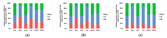
Figure 5.
(a) Emission proportion of different engine types in 2019; (b) Emission proportion of different engine types in 2020; (c) Emission proportion of different engine types in 2021.
As the shore power policy only applies to berthing vessels, for a better analysis of its effectiveness, the operational states of the ships were divided into four categories: transit, manoeuvring, berthing, and anchoring. Figure 6 shows the CO2 emissions of a ship in different states of motion for all types of ships.

Figure 6.
Proportion of different vessels’ status emissions.
As can be seen from the graph, the proportion of emissions from ships in the berthing state decreases significantly in 2020 and 2021, due to further improvements in the shore power policy. The implications of the shore power policy are significant. However, the proportion of emissions from ships in the anchoring state rises, which confirms the increased congestion in the POLB.
Figure 7 depicts many sorts of ships’ waiting times. As can be seen from these graphs, ships are waiting longer in the port area due to decreased productivity. The reason for this is the reduction of workers in the port area due to the pandemic. Congestion in the POLB increases year on year over the three-year period of 2019 to 2021.

Figure 7.
(a) Average waiting time for different ship types at berth; (b) Average waiting time for different ship types at anchorage.
4.4. Uncertainty Factors
Some computational uncertainty exists in this study due to the following:
- (1)
- Issues resulted from the exclusion of data for certain smaller vessels. When processing the AIS data, this study observed that several smaller ships had incomplete AIS data. Inadequate information regarding their operating period or range will result in variation. The inability to accurately anticipate the engine power of tiny vessels also contributes to inaccurate calculations.
- (2)
- Although some missing ship engine data can be calculated using coupled formulas, this procedure contains a certain degree of inaccuracy, which does not ensure the calculation’s precision. For some ships lacking essential parameters such as length, breadth, draught, and design speed, these estimates must be averaged based on similar ship types, which can also result in mistakes.
- (3)
- Weather, waves, and other variables will impact a ship’s fuel use and emissions. In addition, for some vessels with speeds below 0.5 knots, this study assumed that they were sailing under the influence of their engines, neglecting variations in their position and speed caused by weather, waves, etc.
- (4)
- Not all ships utilise the same fuel; therefore, energy variations may influence a ship’s emission parameters. Consequently, it is impossible to monitor the emissions of numerous substances precisely.
4.5. Discussion
In this study, we used AIS data to calculate emissions from POLB-area vessels. The calculation considers variables such as vessel type, size, speed, and engine power, and incorporates factors such as emission factors, sailing patterns, and time of day. We also made assumptions to supplement unavailable data points. To verify the accuracy of our method, we compared the calculations with the POLB official report, using main engine CO2 emissions as an example, which is shown in Table 6.
Table 6.
Comparison of AIS-based calculation and POLB official report results [52].
Using AIS data and a bottom-up approach, this study assesses vessel emissions in the POLB region affected by the COVID pandemic. In terms of vessel type, most vessel types showed a decline. In terms of emissions, there was a slight decrease in 2020, due to a reduction in the number of vessels. However, as the economy starts to recover in 2021, emissions showed a steep increase, with emissions from container ships doubling even more. The reason for this is that ships have to wait longer in port areas, due to the decline in production and the strict controls by the government to prevent the spread of the COVID pandemic. However, despite the longer waiting times for transmission, emissions from ships in the berthing state have decreased, which demonstrates the significance of the shore power policy. The introduction of this policy can significantly reduce emissions from ships in the port area. The main part of the reduction comes from ships in berthing status. Such vessels can switch off their ME, AE, and boilers, and switch to shore power for basic operations, thus achieving zero emissions.
In the future, we envisage that further reductions in emissions in port areas could be achieved by increasing incentives for low-emission vessels and imposing fines or bans on high-emission vessels. As port-wide emissions from ships are caused mainly by ships sitting in port, efforts such as mandating in-port speeds for ships and lowering operational times could be implemented, in addition to shore power restrictions. Moreover, the implementation of electrification in ports can be further pushed in terms of port operations through initiatives such as the construction of marine microgrids, offshore wind power generation, and the expansion of energy storage systems, to promote the use of green energy. Ports should also promote intelligent procedures and implement techniques such as optimising port operations, decreasing vessel waiting times, and enhancing port transport efficiency.
5. Conclusions
The COVID pandemic has affected the shipping industry and the process of achieving environmental sustainability for ships. This study examines the COVID pandemic impact on port-wide ship emissions, using the POLB as an example, and the findings of this study are summarised as follows:
- (1)
- This study gives an optimised approach for calculating ship emissions and proposes a solution to the problem of erroneous emission estimations caused by lacking data for some ships. The method can be applied to future ship emission monitoring and policy design.
- (2)
- This study details the vessel emissions in the POLB region before and after the pandemic. Changes in ship emissions are systematically analysed in four dimensions: different emissions, different ship types, different ship engines, and different ship states.
- (3)
- This study assesses the shore power policy and demonstrates the significance of its implementation through calculations. The implementation of the shore power policy can be extended to many ports in many countries to achieve environmental sustainability development in the shipping industry. We also envisage new rules such as optimising ship scheduling in port areas, changing the flow of port operations, and increasing the demand for fuel. The analysis of emissions for various vessel types and operating modes presented in this study can be used to establish and modify rules.
Lastly, our study has limitations, such as the weather-related variation in the results and the estimating methodologies employed by some vessels with incomplete ship information. In addition, some vessels lack AIS data, and smaller vessels in the port vicinity may disable their AIS equipment. In future research, satellite remote sensing and radar data can be employed to measure ship emissions more precisely.
Author Contributions
Methodology, Z.H., J.S.L.L. and M.L.; Software, Z.H. and M.L.; Conceptualisation, J.S.L.L.; Visualisation, Z.H.; Writing—origin and editing, Z.H.; Validation, J.S.L.L.; Writing—review and editing, J.S.L.L.; Supervision, J.S.L.L.; Formal analysis, M.L.; Investigation, M.L. All authors have read and agreed to the published version of the manuscript.
Funding
Project 04SBS000097C120 at Nanyang Technological University, Singapore.
Institutional Review Board Statement
Not applicable.
Informed Consent Statement
Not applicable.
Data Availability Statement
Data analysed during this study are available from the corresponding author upon request.
Conflicts of Interest
The authors declare no conflict of interest.
References
- Guo, S.; Zheng, S.; Hu, Y.; Hong, J.; Wu, X.; Tang, M. Embodied energy use in the global construction industry. Appl. Energy 2019, 256, 113838. [Google Scholar] [CrossRef]
- Poulsen, R.T.; Ponte, S.; Sornn-Friese, H. Environmental upgrading in global value chains: The potential and limitations of ports in the greening of maritime transport. Geoforum 2018, 89, 83–95. [Google Scholar] [CrossRef]
- Yang, D.; Wu, L.; Wang, S.; Jia, H.; Li, K.X. How big data enriches maritime research—A critical review of Automatic Identification System (AIS) data applications. Transp. Rev. 2019, 39, 755–773. [Google Scholar] [CrossRef]
- Sui, C.; de Vos, P.; Stapersma, D.; Visser, K.; Ding, Y. Fuel consumption and emissions of ocean-going cargo ship with hybrid propulsion and different fuels over voyage. J. Mar. Sci. Eng. 2020, 8, 588. [Google Scholar] [CrossRef]
- Ytreberg, E.; Åström, S.; Fridell, E. Valuating environmental impacts from ship emissions–The marine perspective. J. Environ. Manag. 2021, 282, 111958. [Google Scholar] [CrossRef] [PubMed]
- Gan, L.; Che, W.; Zhou, M.; Zhou, C.; Zheng, Y.; Zhang, L.; Rangel-Buitrago, N.; Song, L. Ship exhaust emission estimation and analysis using Automatic Identification System data: The west area of Shenzhen port, China, as a case study. Ocean Coast. Manag. 2022, 226, 106245. [Google Scholar] [CrossRef]
- Notteboom, T.; Lam, J.S.L. The greening of terminal concessions in seaports. Sustainability 2018, 10, 3318. [Google Scholar] [CrossRef]
- Iris, Ç.; Lam, J.S.L. A review of energy efficiency in ports: Operational strategies, technologies and energy management systems. Renew. Sustain. Energy Rev. 2019, 112, 170–182. [Google Scholar] [CrossRef]
- Xin, J.; Negenborn, R.R.; Lodewijks, G. Event-driven receding horizon control for energy-efficient container handling. Control Eng. Pract. 2015, 39, 45–55. [Google Scholar] [CrossRef]
- Zhou, Y.; Zhang, Y.; Ma, D.; Lu, J.; Luo, W.; Fu, Y.; Li, S.; Feng, J.; Huang, C.; Ge, W.; et al. Port-Related Emissions, Environmental Impacts and Their Implication on Green Traffic Policy in Shanghai. Sustainability 2020, 12, 4162. [Google Scholar] [CrossRef]
- Bermúdez, F.M.; Laxe, F.G.; Aguayo-Lorenzo, E. Assessment of the tools to monitor air pollution in the Spanish ports system. Air Qual. Atmos. Health 2019, 12, 651–659. [Google Scholar] [CrossRef]
- Alamoush, A.S.; Ölçer, A.I.; Ballini, F. Port greenhouse gas emission reduction: Port and public authorities’ implementation schemes. Res. Transp. Bus. Manag. 2022, 43, 100708. [Google Scholar] [CrossRef]
- Shrestha, N.; Shad, M.Y.; Ulvi, O.; Khan, M.H.; Karamehic-Muratovic, A.; Nguyen, U.-S.D.; Baghbanzadeh, M.; Wardrup, R.; Aghamohammadi, N.; Cervantes, D. The impact of COVID-19 on globalization. One Health 2020, 11, 100180. [Google Scholar] [CrossRef]
- Shi, K.; Weng, J. Impacts of the COVID-19 epidemic on merchant ship activity and pollution emissions in Shanghai port waters. Sci. Total Environ. 2021, 790, 148198. [Google Scholar] [CrossRef] [PubMed]
- March, D.; Metcalfe, K.; Tintoré, J.; Godley, B.J. Tracking the global reduction of marine traffic during the COVID-19 pandemic. Nat. Commun. 2021, 12, 2415. [Google Scholar] [CrossRef]
- Miola, A.; Ciuffo, B. Estimating air emissions from ships: Meta-analysis of modelling approaches and available data sources. Atmos. Environ. 2011, 45, 2242–2251. [Google Scholar] [CrossRef]
- Wan, Z.; Ji, S.; Liu, Y.; Zhang, Q.; Chen, J.; Wang, Q. Shipping emission inventories in China’s Bohai Bay, Yangtze River Delta, and Pearl River Delta in 2018. Mar. Pollut. Bull. 2020, 151, 110882. [Google Scholar] [CrossRef]
- Weng, J.; Shi, K.; Gan, X.; Li, G.; Huang, Z. Ship emission estimation with high spatial-temporal resolution in the Yangtze River estuary using AIS data. J. Clean. Prod. 2020, 248, 119297. [Google Scholar] [CrossRef]
- Yin, Y.; Lam, J.S.L.; Tran, N.K. Emission accounting of shipping activities in the era of big data. Int. J. Shipp. Transp. Logist. 2021, 13, 156–184. [Google Scholar] [CrossRef]
- Livaniou, S.; Chatzistelios, G.; Lyridis, D.V.; Bellos, E. LNG vs. MDO in Marine Fuel Emissions Tracking. Sustainability 2022, 14, 3860. [Google Scholar] [CrossRef]
- Eggleston, H.; Buendia, L.; Miwa, K.; Ngara, T.; Tanabe, K. 2006 IPCC Guidelines for National Greenhouse Gas Inventories. 2006. Available online: https://www.ipcc-nggip.iges.or.jp/public/2006gl (accessed on 10 January 2023).
- Kesgin, U.; Vardar, N. A study on exhaust gas emissions from ships in Turkish Straits. Atmos. Environ. 2001, 35, 1863–1870. [Google Scholar] [CrossRef]
- Brioude, J.; Kim, S.W.; Angevine, W.M.; Frost, G.; Lee, S.H.; McKeen, S.; Trainer, M.; Fehsenfeld, F.C.; Holloway, J.; Ryerson, T. Top-down estimate of anthropogenic emission inventories and their interannual variability in Houston using a mesoscale inverse modeling technique. J. Geophys. Res. Atmos. 2011, 116, D2035. [Google Scholar] [CrossRef]
- Browning, L.; Bailey, K. Current Methodologies and Best Practices for Preparing Port Emission Inventories. ICF Consulting Report to Environmental Protection Agency. 2006. Available online: https://www3.epa.gov/ttnchie1/conference/ei15/session1/browning.pdf (accessed on 19 September 2022).
- Jalkanen, J.-P.; Brink, A.; Kalli, J.; Pettersson, H.; Kukkonen, J.; Stipa, T. A modelling system for the exhaust emissions of marine traffic and its application in the Baltic Sea area. Atmos. Chem. Phys. 2009, 9, 9209–9223. [Google Scholar] [CrossRef]
- Goldsworthy, L.; Goldsworthy, B. Modelling of ship engine exhaust emissions in ports and extensive coastal waters based on terrestrial AIS data—An Australian case study. Environ. Model. Softw. 2015, 63, 45–60. [Google Scholar] [CrossRef]
- Huang, L.; Wen, Y.; Geng, X.; Zhou, C.; Xiao, C.; Zhang, F. Estimation and spatio-temporal analysis of ship exhaust emission in a port area. Ocean Eng. 2017, 140, 401–411. [Google Scholar] [CrossRef]
- Chen, Q.; Ge, Y.-E.; Lau, Y.-y.; Dulebenets, M.A.; Sun, X.; Kawasaki, T.; Mellalou, A.; Tao, X. Effects of COVID-19 on passenger shipping activities and emissions: Empirical analysis of passenger ships in Danish waters. Marit. Policy Manag. 2022, 1–21. [Google Scholar] [CrossRef]
- Durán-Grados, V.; Amado-Sánchez, Y.; Calderay-Cayetano, F.; Rodríguez-Moreno, R.; Pájaro-Velázquez, E.; Ramírez-Sánchez, A.; Sousa, S.I.; Nunes, R.A.; Alvim-Ferraz, M.C.; Moreno-Gutiérrez, J. Calculating a drop in carbon emissions in the Strait of Gibraltar (Spain) from domestic shipping traffic caused by the COVID-19 crisis. Sustainability 2020, 12, 10368. [Google Scholar] [CrossRef]
- Čurović, L.; Jeram, S.; Murovec, J.; Novaković, T.; Rupnik, K.; Prezelj, J. Impact of COVID-19 on environmental noise emitted from the port. Sci. Total Environ. 2021, 756, 144147. [Google Scholar] [CrossRef]
- Mocerino, L.; Quaranta, F. How emissions from cruise ships in the port of Naples changed in the COVID-19 lock down period. Proc. Inst. Mech. Eng. Part M J. Eng. Marit. Environ. 2022, 236, 125–130. [Google Scholar] [CrossRef]
- Mujal-Colilles, A.; Guarasa, J.N.; Fonollosa, J.; Llull, T.; Castells-Sanabra, M. COVID-19 impact on maritime traffic and corresponding pollutant emissions. The case of the Port of Barcelona. J. Environ. Manag. 2022, 310, 114787. [Google Scholar] [CrossRef]
- Campisi, T.; Marinello, S.; Costantini, G.; Laghi, L.; Mascia, S.; Matteucci, F.; Serrau, D. Locally integrated partnership as a tool to implement a Smart Port Management Strategy: The case of the port Ravenna (Italy). Ocean Coast. Manag. 2022, 224, 106179. [Google Scholar] [CrossRef]
- Marinello, S.; Balugani, E.; Rimini, B. Sustainability of logistics infrastructures: Operational and technological alternatives to reduce the impact on air quality. In Proceedings of the 26th Summer School Francesco Turco, Online, 8–10 September 2021. [Google Scholar]
- Xin, X.; Liu, K.; Yang, X.; Yuan, Z.; Zhang, J. A simulation model for ship navigation in the “Xiazhimen” waterway based on statistical analysis of AIS data. Ocean Eng. 2019, 180, 279–289. [Google Scholar] [CrossRef]
- Zhang, L.; Meng, Q.; Xiao, Z.; Fu, X. A novel ship trajectory reconstruction approach using AIS data. Ocean Eng. 2018, 159, 165–174. [Google Scholar] [CrossRef]
- Winebrake, J.J.; Corbett, J.; Green, E.; Lauer, A.; Eyring, V. Mitigating the health impacts of pollution from oceangoing shipping: An assessment of low-sulfur fuel mandates. Environ. Sci. Technol. 2009, 43, 4776–4782. [Google Scholar] [CrossRef]
- Cepowski, T. Regression formulas for the estimation of engine total power for tankers, container ships and bulk carriers on the basis of cargo capacity and design speed. Pol. Marit. Res. 2019, 26, 82–94. [Google Scholar] [CrossRef]
- Huang, L.; Wen, Y.; Zhang, Y.; Zhou, C.; Zhang, F.; Yang, T. Dynamic calculation of ship exhaust emissions based on real-time AIS data. Transp. Res. Part D Transp. Environ. 2020, 80, 102277. [Google Scholar] [CrossRef]
- IMO. Fleet and CO2 Calculator: GreenVoyage2050. Available online: https://greenvoyage2050.imo.org/fleet-and-co2-calculator (accessed on 27 November 2022).
- Chen, D.; Wang, X.; Li, Y.; Lang, J.; Zhou, Y.; Guo, X.; Zhao, Y. High-spatiotemporal-resolution ship emission inventory of China based on AIS data in 2014. Sci. Total Environ. 2017, 609, 776–787. [Google Scholar] [CrossRef]
- Yau, P.; Lee, S.; Corbett, J.J.; Wang, C.; Cheng, Y.; Ho, K. Estimation of exhaust emission from ocean-going vessels in Hong Kong. Sci. Total Environ. 2012, 431, 299–306. [Google Scholar] [CrossRef]
- Ng, S.K.; Loh, C.; Lin, C.; Booth, V.; Chan, J.W.; Yip, A.C.; Li, Y.; Lau, A.K. Policy change driven by an AIS-assisted marine emission inventory in Hong Kong and the Pearl River Delta. Atmos. Environ. 2013, 76, 102–112. [Google Scholar] [CrossRef]
- Knežević, V.; Radonja, R.; Dundović, Č. Emission inventory of marine traffic for the port of zadar. Pomorstvo 2018, 32, 239–244. [Google Scholar] [CrossRef]
- Hu, Q.-M.; Hu, Z.-H.; Du, Y. Berth and quay-crane allocation problem considering fuel consumption and emissions from vessels. Comput. Ind. Eng. 2014, 70, 1–10. [Google Scholar] [CrossRef]
- IMO. Prevention of Air Pollution from Ships. Available online: https://www.imo.org/en/ourwork/environment/pages/air-pollution.aspx (accessed on 30 November 2022).
- CARB. California Air Resources Board: Marine Notice 2020-2. Available online: https://ww2.arb.ca.gov/sites/default/files/2020-10/marine_notice_2020-2_final_ADA.pdf (accessed on 30 November 2022).
- Comer, B.; Olmer, N.; Mao, X.; Roy, B.; Rutherford, D. Prevalence of Heavy Fuel Oil and Black Carbon in Arctic Shipping, 2015 to 2025. 2017. Available online: https://theicct.org/publication/prevalence-of-heavy-fuel-oil-and-black-carbon-in-arctic-shipping-2015-to-2025 (accessed on 3 November 2022).
- POLB. Port Info: Overview: About the Port. 2020. Available online: https://polb.com/port-info (accessed on 27 October 2022).
- POLB. TEUS Archive: 1995 to Present by Year. 2022. Available online: https://polb.com/business/port-statistics/#latest-statistics (accessed on 27 October 2022).
- CARB. Shore Power Regulation Fact Sheet. 2014. Available online: https://polb.com/environment/shore-power/#shore-power-program-details (accessed on 27 October 2022).
- POLB. Air Emissions Inventory. 2023. Available online: https://polb.com/environment/air/#emissions-inventory (accessed on 1 April 2023).


Disclaimer/Publisher’s Note: The statements, opinions and data contained in all publications are solely those of the individual author(s) and contributor(s) and not of MDPI and/or the editor(s). MDPI and/or the editor(s) disclaim responsibility for any injury to people or property resulting from any ideas, methods, instructions or products referred to in the content. |
© 2023 by the authors. Licensee MDPI, Basel, Switzerland. This article is an open access article distributed under the terms and conditions of the Creative Commons Attribution (CC BY) license (https://creativecommons.org/licenses/by/4.0/).