Multi-Objective Optimization of Envelope Design of Rural Tourism Buildings in Southeastern Coastal Areas of China Based on NSGA-II Algorithm and Entropy-Based TOPSIS Method

Abstract

The rapid development of rural tourism and higher requirements for the indoor environments of rural tourism buildings (RTBs) have led to rapid growth in the energy consumption of RTBs. The aim of this work was to apply a new method to optimize the indoor thermal environments and energy performances of RTBs and promote scientific passive design strategies for RTBs in southeastern coastal areas of China. First, a field survey was carried out to understand the statuses of buildings and the energy consumption of RTBs. Through a building typology analysis, two types of RTBs (renovated from existing buildings and newly built) were chosen as the dominant types in the villages. Second, a comprehensive parametric study was conducted to examine the impact of energy consumption and the indoor thermal environment using a global sensitivity analysis. The passive design parameters with large sensitivity impacts were selected using the Sobol sampling method and by calculating the comprehensive contribution rates of the parameters. Then, the NSGA-II algorithm was used to simultaneously minimize the two objectives and generate the Pareto front solution sets of the two RTB types. Finally, by applying an entropy-based TOPSIS decision-making method, the optimal schemes (the best energy-saving solution, the best comfort solution, and the best compromise solution) for the two RTB types were further obtained from the feasible Pareto-optimal solutions, and the suggested values for the design parameters are presented. This study proposes a new multi-objective optimization approach combining the NSGA-II algorithm and an entropy-based TOPSIS decision-making method, and the findings are valuable, as they can help designers to improve the designs of rural tourism buildings.

1. Introduction

1.1. Background

With the rapid development of the economy and urbanization, a growing number of urban residents in China want to spend weekends and holidays in the suburbs or rural areas [1]. Official statistics show that by the end of 2019 (before the epidemic), the number of rural tourism (RT) receptions in China reached 3.09 billion and the annual income of RT was nearly CNY 850 billion [2]. In order to further improve the quality and level of RT development, the Ministry of Culture and Tourism and the National Development and Reform Commission jointly issued 1200 excellent RT demonstration villages as key villages of RT in China [3]. As an important part of the tourism industry in China, RT is regarded as an important driving force for China’s rural economic growth [4]. Therefore, under the background of the rapid development of RT in China, more and more villagers are transforming their buildings with single residential functions into rural tourism buildings (RTBs) providing tourism residences, catering services, leisure, and entertainment.

In addition, the development of the new rural reconstruction in China also impels the energy-saving work extending from cities and towns to rural areas [5]. Many scientific studies have been carried out on the indoor environments and energy conservation of rural residential buildings (RRBs) [6,7,8], but few studies have been carried out on RTBs. As small accommodation facilities where villagers use their own RRBs to provide accommodations and leisure activities for tourists, RTBs have different functions than ordinary RRBs [9]. Additionally, RTBs require higher indoor comfort, which also leads to higher building energy consumption [10]. Furthermore, the Ministry of Culture and Tourism, together with the Ministry of Ecological Environment and other relevant departments in China, put forward the design principle of “insisting on ecological priority” for RTBs to advocate energy conservation and environmental protection [4]. Hence, the scientific analysis of the energy-saving strategies of RTBs is conducive to promoting the development of energy conservation and environmental protection in rural areas of China and can provide scientific guidance for RTB design.

1.2. Indoor Thermal Environment and Energy Consumption of RTBs

Although few studies have been carried out on the indoor environments and building energy consumption of RTBs, many studies have been carried out on ordinary RRBs. Tsinghua University conducted comprehensive and in-depth field investigations on ordinary RRBs in China from 2006 to 2007. The results showed that both the thermal performance of building envelopes and the indoor thermal comfort of ordinary RRBs were poor in south China [11]. In particular, the degree of dissatisfaction with the indoor thermal environments was higher in summer than that in winter. Studies more than ten years later revealed that the indoor thermal environments of ordinary RRBs still could not meet the requirements of Chinese standards [12], even in newly built RRBs where the performance of the building envelope and air tightness had been improved [13].

Meanwhile, many studies have confirmed the fact that the energy consumption of RRBs is increasing and even has a tendency to exceed that of urban residential buildings [11]. Using the China Building Energy and Emission Model (CBEEM), the Building Energy Research Center (BERC) of Tsinghua University estimated that the energy consumption of ordinary RRBs in 2020 was 229 million tce, accounting for 22% of the total building energy consumption in China, including 344.6 billion kWh of electricity consumption [14]. Using field surveys of rural households, Li et al. [6] and Cao et al. [15] attributed the rapid increase in the commercial energy consumption of ordinary RRBs to the improvement of living standards [16] and the clean transformation of the rural energy structure [17].

Compared to urban residential buildings (URBs) and public buildings, the thermal performance of RTBs is poor. This is mainly because the energy-saving design standards for URBs and public buildings are mandatory standards, while the standards for RRBs are voluntary. As shown in Table 1, the building envelope requirements of URBs and public buildings are higher than those of RRBs. Although the current energy consumption of RTBs is lower than URBs and public buildings, this is mainly because of the small permanent population of rural households, the young and middle-aged labor force going out for work, and less time at home [10]. With the implementation of China’s rural revitalization strategy, this situation would gradually change.

To provide tourists with the experience of local nature, culture, production, and life using idle rural residential resources in rural areas [18], RTBs have the dual characteristics of RRBs and hotels. As RTBs have building shapes, plane layouts, and structural levels similar to ordinary RRBs [9], RTBs also have the same indoor environment and energy consumption problems as ordinary RRBs. Xi et al. [19] investigated the energy consumption structure of rural households in scenic spots, and the results showed that the total energy consumption per capita of RTBs was 42.96% higher than that of ordinary RTBs. The results in Section 2.1.2 also draw similar conclusions. At present, the average annual energy consumption of small public buildings in China is about 60 Kwh/m² [11]. According to the official monitoring data of tourism buildings in Shanghai, the average building energy consumption of hotels and restaurants was above 100 Kwh/m² from 2017 to 2019, even reaching 130.5 Kwh/m² [20]. Air conditioning accounted for 33% of energy consumption. It can be predicted that with the continuous development of RT, the energy consumption of RTBs would be huge. The abovementioned research indicates that most RTBs have the problems of poor indoor thermal environments and high building energy consumption at present due to a lack of scientific design. Zhu et al. [9] optimized the designs of RTB shapes and the window-to-wall ratio in north China. However, there is no research on the passive design of the building envelopes of RTBs in southeastern coastal areas of China.

Table 1. Comparison of thermal requirements of building envelopes of different types of buildings in Chinese standards.

Building Types		Requirements	Standards
		Roof: U ≤ 0.8~1.0 W/(m2·K) External wall: U ≤ 1.5~1.8 W/(m2·K) Door: U ≤ 3.0 W/(m2·K) Window: U ≤ 3.2~4.7 W/(m2·K)	GB/T 50824-2013 [21] Voluntary
RTBs	Ordinary RRBs
		Roof: U ≤ 0.4 W/(m2·K) External wall: U ≤ 0.6~1.2 W/(m2·K) Window: U ≤ 2.0~2.8 W/(m2·K); SHGC ≤ 0.5 (winter)/0.25~0.4 (summer) Door: U ≤ 2.0 W/(m2·K) Floor: U ≤ 1.8 W/(m2·K)	GB 55015-2021 [22] Mandatory
URBs
		Roof: U ≤ 0.4 W/(m2·K) External wall: U ≤ 0.6~0.8 W/(m2·K) Window: U ≤ 3.0~1.8 W/(m2·K); SHGC ≤ 0.45~0.20 Floor: U ≤ 0.7 W/(m2·K)	GB 55015-2021 [22] Mandatory
Hotels and Restaurants (building area ≥ 300 m2)

Table 1. Comparison of thermal requirements of building envelopes of different types of buildings in Chinese standards.

Building Types		Requirements	Standards
		Roof: U ≤ 0.8~1.0 W/(m2·K) External wall: U ≤ 1.5~1.8 W/(m2·K) Door: U ≤ 3.0 W/(m2·K) Window: U ≤ 3.2~4.7 W/(m2·K)	GB/T 50824-2013 [21] Voluntary
RTBs	Ordinary RRBs
		Roof: U ≤ 0.4 W/(m2·K) External wall: U ≤ 0.6~1.2 W/(m2·K) Window: U ≤ 2.0~2.8 W/(m2·K); SHGC ≤ 0.5 (winter)/0.25~0.4 (summer) Door: U ≤ 2.0 W/(m2·K) Floor: U ≤ 1.8 W/(m2·K)	GB 55015-2021 [22] Mandatory
URBs
		Roof: U ≤ 0.4 W/(m2·K) External wall: U ≤ 0.6~0.8 W/(m2·K) Window: U ≤ 3.0~1.8 W/(m2·K); SHGC ≤ 0.45~0.20 Floor: U ≤ 0.7 W/(m2·K)	GB 55015-2021 [22] Mandatory
Hotels and Restaurants (building area ≥ 300 m2)

1.3. Studies on Multi-Objective Optimization of Building Performance

In the process of architectural design, the optimization of design schemes directly affects the green performances of buildings and building facades [23,24]. Design parameters (independent variables) and building performance (dependent variables) are often high-dimensional. Therefore, they are difficult to compare and select by artificial means due to the large amount of calculation and the difficulty of design decisions. With the development of science and technology, the multiple-objective optimization (MOO) method of using performance simulation and algorithm optimization to optimize the performance of buildings with two or three objectives is widely used in architectural design. One of the MOO methods is based on the interaction between mathematical software (such as MATLAB or Python) and energy consumption simulation software (such as EnergyPlus, TRNSYS, or ESP-r). The cross-platform interaction between the two programs requires a joint simulation interface, e.g., jeplus or DesignBuilder. Since it can only be associated with energy consumption simulation software, the optimization performance mainly focuses on energy savings, carbon emissions, comfort, and economy. Furthermore, it cannot change the building geometry or layout, as the parametric analysis is based on a specific reference building model [25]. For example, Chen et al. [26] proposed an integrated optimization framework to explore the minimum building carbon emissions, indoor discomfort hours, and global cost of building based on the Python platform. Ciardiello et al. [27] adopted a new approach based on Python intertwined with EnergyPlus by means of the Eppy library to facilitate the optimization of shapes and envelopes in building energy design. Ascione et al. [28] addressed the building envelope design to minimize energy consumption, global cost, and thermal discomfort in different Italian climatic zones by means of the coupling between EnergyPlus and MATLAB. Abdou et al. [29] used TRNSYS coupled with MOBO [30] to assess the best solution.

Another method is based on the parametric design platform Rhinoceros, integrating plugins (e.g., Grasshopper, Octopus, Ladybug, and Honeybee) for geometric modeling, performance simulation, evaluation, and optimization. In addition to the simulations carried out by energy consumption simulation software, the rich plugins can perform other simulations, such as lighting analysis, and they can also change the dimensions of the model. This method is widely used by many scholars to optimize building shapes or component sizes. Zhu et al. [9] applied this method to explore early designs of building shape and the window-to-wall ratio. Ebrahimi-Moghadam et al. [31] optimized internal light shelves for residential buildings, while Wang et al. [24] and Fan et al. [23] optimized the external shading of a classroom and gymnasium, respectively.

The abovementioned intelligent optimization methods are all based on genetic algorithms that automatically search for a solution. Among them, the NSGA-II [29,32] and NSGA-III [26,33] algorithms are the most widely used. On this basis, Ciardiello et al. [27] took aNSGA-II (a peculiar version of NSGA-II) and Mostafazadeh et al. [33] used prNSGA-III (a modified version of NSGA-III) as optimization algorithms for research. Other algorithms such as SPEA-II [9,23], HypE [9,34], MOPSO, and MOEA/E have also been applied [26,35]. Additionally, previous work mentioned above dealt with ordinary residential buildings [27,36], zero/low-energy buildings [37,38,39,40], commercial buildings [41], office buildings [26], etc. Li et al. [9] applied MOO to promote the scientific design of RTBs in north China with regards to energy consumption, daylighting, and thermal comfort performance. However, few studies have focused on the optimal passive strategies for RTBs.

A genetic algorithm obtains a series of solutions distributed on a Pareto front surface whose comprehensive performances are more advantageous than other generations. Faced with numerous feasible Pareto solutions, Ebrahimi-Moghadam et al. [31] applied the LINAMP method to find the optimal design of light shelves. Zhu et al. [9] and Ciardiello et al. [27] obtained the optimal solutions using the utopian point method. Chen et al. [26] proposed an improved optimal balance formula based on the utopian point method to obtain the optimal balance schemes of building carbon emissions, indoor discomfort hours, and the global costs of buildings. The studies above were based on the calculation of the Euclidean distance between the Pareto front sets and the ideal point to determine the best solution from the Pareto solution sets, but the importance of different objectives was not considered. Luo et al. [34] considered the weights of the objectives in their study but assumed an equal importance. In fact, the weights of multiple objectives are not all the same. Mostafazadeh et al. [33] adopted the TOPSIS method to choose the final strategy. This method is a useful technique for dealing with multi-attribute or multi-criteria decision-making problems in the real world [42] to seek the equilibrium points for multi-objective games, considering the weight of each objective. In this work, an entropy weight TOPSIS method is applied to obtain the optimal solution from Pareto front solutions.

Sensitivity analysis (SA), as a method to identify the relative influences of input parameters, has been widely used in automatic control, economy, and other fields [43]. In the building sector, SA is widely applied in the first step of building performance optimization [44], which can be used to identify important variables and narrow the range of values. Tian [45] and Pang et al. [43] reviewed the application of SA methods in building performance analysis. SA methods can be divided into local and global approaches. A local SA only checks the influence of a single input variable on the model; hence, it is easy to calculate and operate [39]. The global approach simultaneously calculates the comprehensive effects of all uncertain inputs. Therefore, it is considered to be one of the more effective and highly accurate analysis methods for building energy performance analysis. A classical global SA includes a regression method (SRC, SRRC, and t-value), a screening method (Morris), a meta-model method (MARS, SVM, and GP), a variance method (Fast and Sobol), etc. Zhang et al. [46] studied the key factors affecting the energy consumption of net-zero energy buildings using the regression analysis method (SRC method). Bre et al. [47], Tushar et al. [48], and Maučec et al. [49] used the Morris screening method to carry out sensitivity analyses. Li et al. and Naji et al. [50] adopted a variety of methods for com [51] parative analysis. From these above reviews, it can be concluded that global SA methods can effectively identify key parameters. A regression analysis indicates how a typical value of an output changes when any of the input variables is varied (assuming that the input variables are independent of each other). Therefore, in this paper, the regression method was selected due to its rapidity, simplicity, and lower data requirement [45,46].

1.4. Aims of the Research

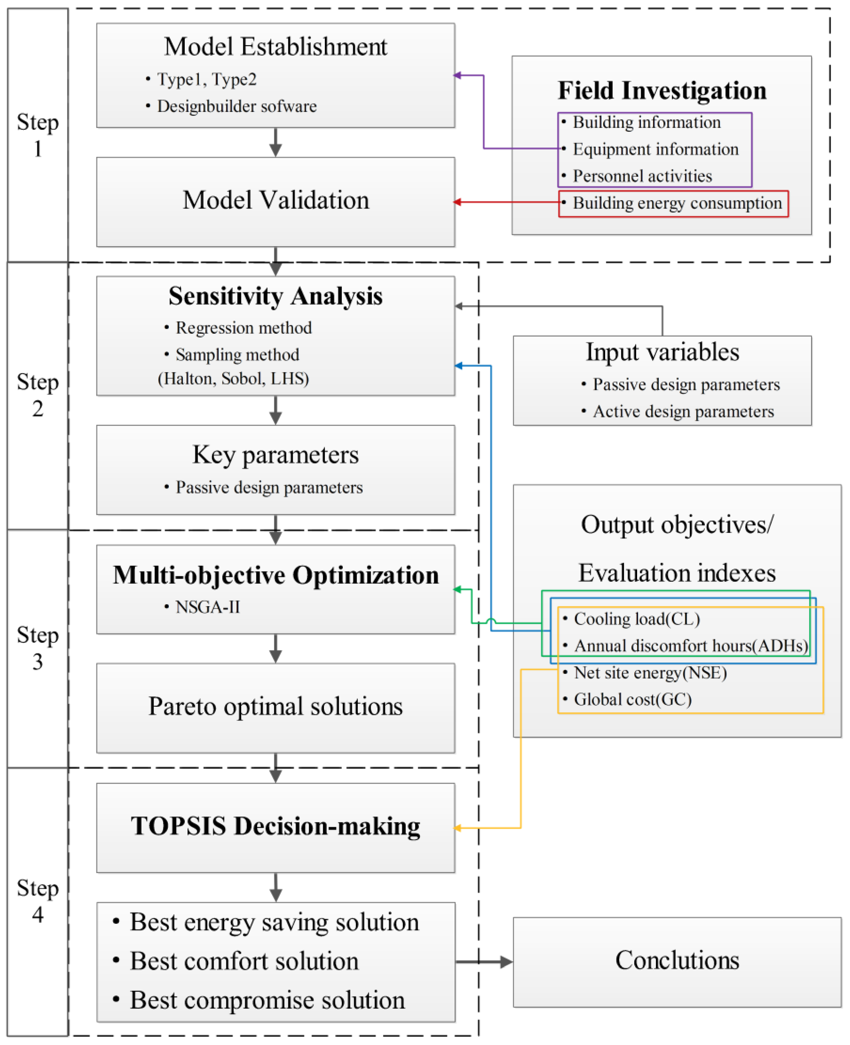
Under the background of extensive development of RT and the rapid growth of RTBs, the higher requirements of indoor environments will lead to higher energy consumption. The aim of this study was to draw attention to the practical status and promote the scientific passive design strategies of RTBs in southeastern coastal areas of China for better building performance in terms of the energy consumption and indoor thermal environment. A global sensitivity analysis method was applied to analyze the factors influencing the indoor thermal comfort and building energy consumption of RTBs. A new multi-objective optimization method is proposed based on the NSGA-II algorithm and an entropy-based TOPSIS decision-making method to obtain the optimal passive design parameters of RTBs, which can also facilitate better decision making related to the RTB design in southeastern coastal areas of China.

2. Methodology

A flow chart of this work is shown in Figure 1. The major process can be divided into four steps. Generally speaking, step one is to carry out a field investigation to understand the basic situation of RTBs. Then, typical models are established and validated. Step two is to apply an SA to obtain key passive design parameters for MOO. Step three is to operate MOO and generate the Pareto front sets. Step four is to use the TOPSIS decision-making method to choose the optimal solutions.

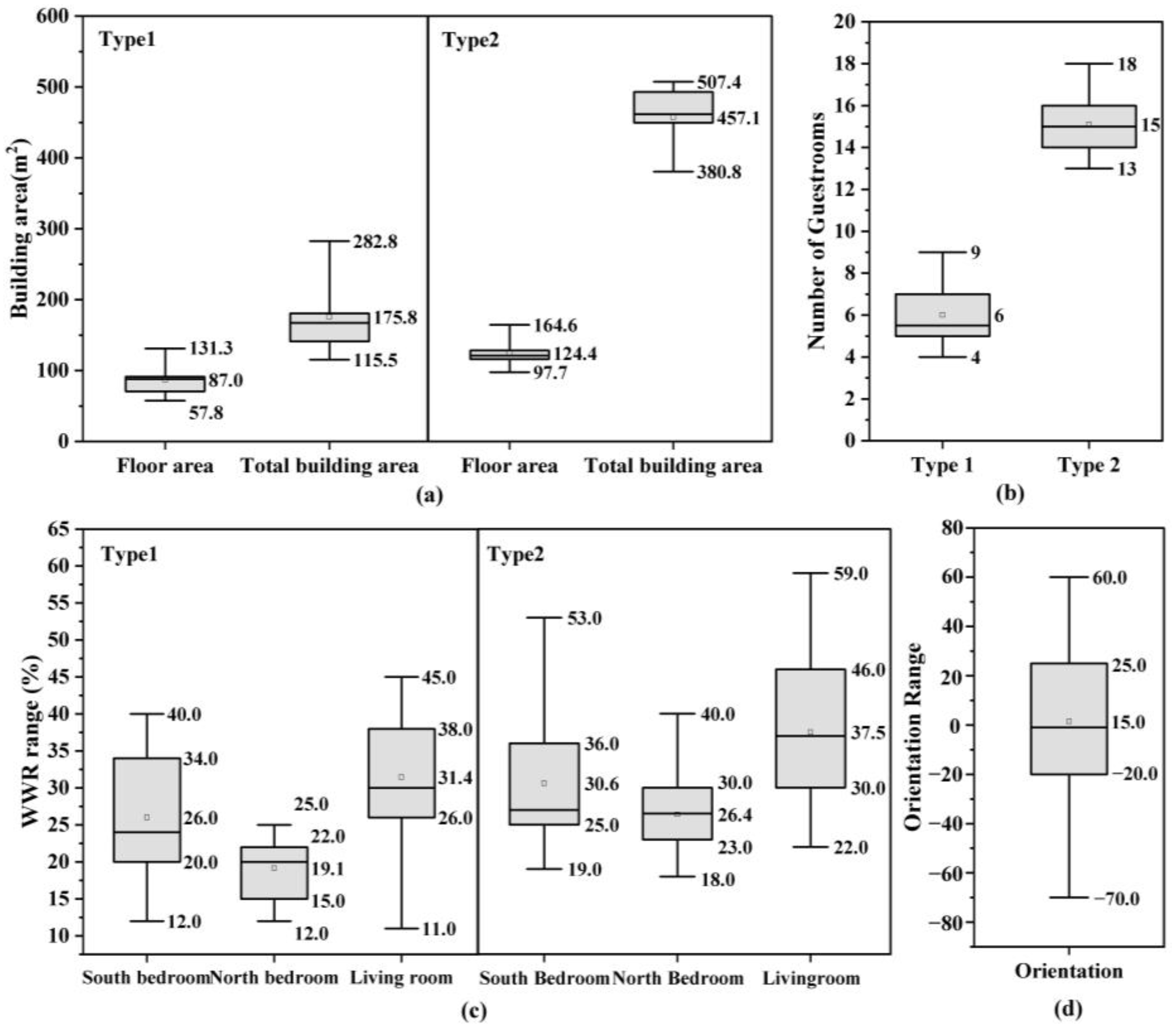
2.1. Field Survey of RTBs

In recent years, RT in China has developed rapidly, particularly in the southeastern coastal areas of China, which are not only economically developed but also rich in RT resources. Among them, Zhejiang Province ranks first and is one of the most developed and mature RT provinces in China [2]. Among the national key rural tourism villages announced from 2019 to 2022, a total of 48 villages in Zhejiang Province were selected, ranking at the forefront of the whole country [3]. Therefore, RTBs in Zhejiang province represent the typical mode in southeastern coastal areas of China and are thus worth studying. The Zhoushan islands (longitude 121°30′ to 123°25′, latitude 29°32′ to 31°04′) are located on the southeastern coast of Zhejiang Province, close to Shanghai, Hangzhou, other large and medium-sized cities, and the Yangtze River Delta, and have rich RT resources and an outstanding position. Additionally, the Zhoushan islands were also one of the earliest areas to carry out RT, with a history of more than 20 years, and several villages made the list of national key rural tourism villages. Therefore, a study of RTBs in the Zhoushan islands is representative. Based on the research purpose, the selected RTB samples needed to meet the following criteria:

(1)

The RTBs were farmers’ self-built and self-occupied houses.

(2)

The RT business operators were the farmers themselves.

(3)

The RT business had been carried out for more than 5 years and had a high occupancy rate.

(4)

The RTBs had similar housing equipment systems.

(5)

The business operators were willing to allow energy monitors and other measuring equipment to be installed in guestrooms.

(6)

The business operators were willing to provide guest information such as gender, age, and check-in and check-out times.

Through a preliminary survey on the characteristics of building styles, building layouts, building structures and materials, building years, and so on, it was found that RTBs in local villages have strong similarities in their building forms. Using a typology analysis, the RTBs could be divided into two types:

Type 1: two-story stone–concrete RTBs built before 2000 and renovated from existing RRBs.

Type 2: four-story brick–concrete or frame-structure RTBs that were newly built after 2000 considering the RT business.

Additionally, most type 1 RTBs have double-pitched roofs, and most type 2 RTBs have flat roofs.

Finally, ten RTBs of each type were surveyed. To make the typical RTBs representative of most RTBs, the targets of the investigation were randomly sampled and met the criteria mentioned above. A detailed investigation, including field measurements and questionnaire surveys, was carried out to determine the basic information of RTBs, energy systems and energy consumption, and the energy-use behavior of tourists and RT operators. The dimensions of RTBs, such as the plane layout, floor height, doors and windows, and orientation were mapped in detail. The household characteristics, appliances, and energy consumption were determined using face-to-face interviews. Furthermore, measuring equipment with recording functions (e.g., energy monitors and thermo-hygrometers) were also installed in guestrooms and other important zones to record the personnel’s energy use and behavior characteristics.

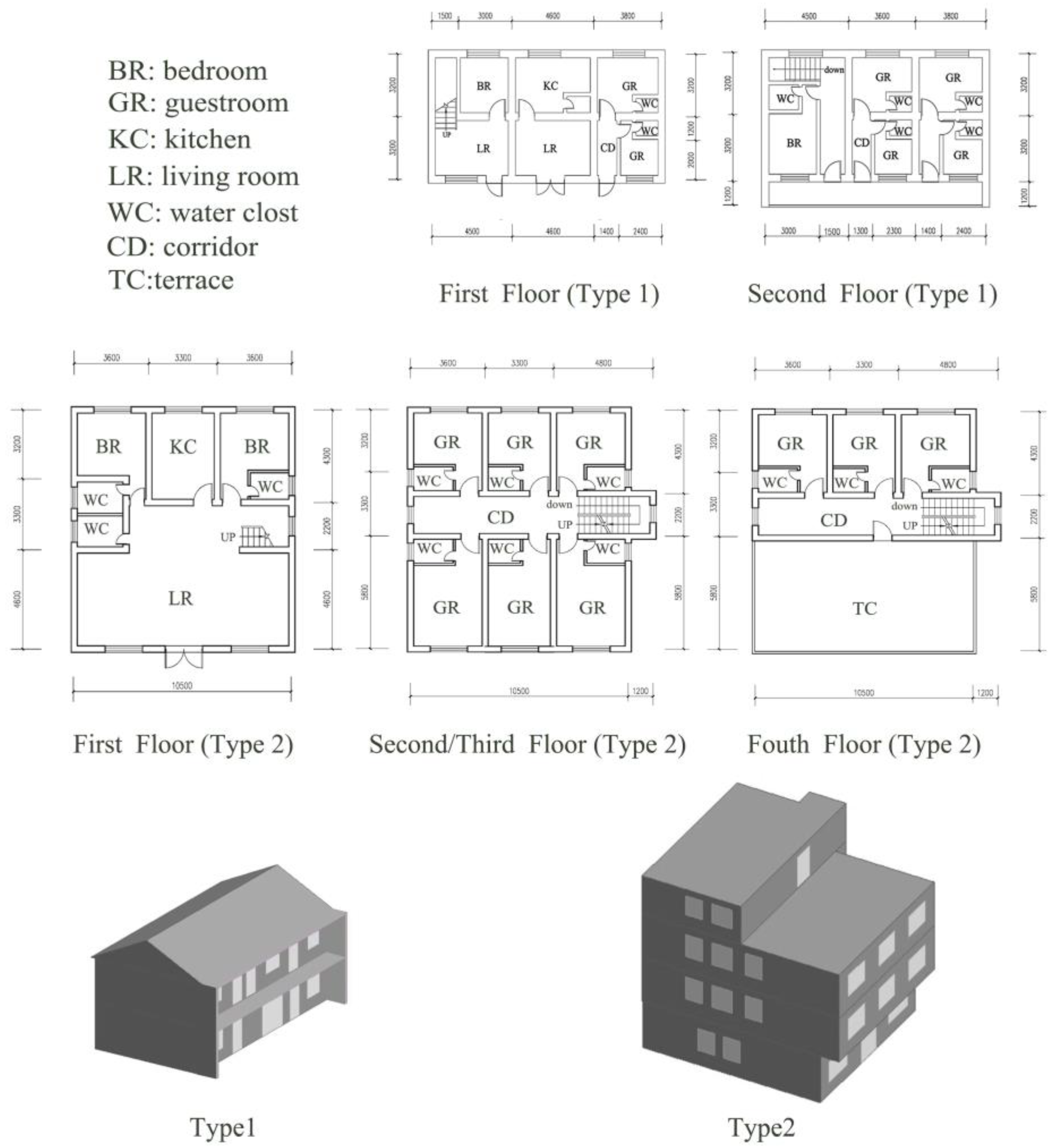
2.1.1. The Building Characteristics of RTBs

The dimensions of the building area, doors, windows, orientation, and number of guestrooms were obtained from the survey of the RTB planning status. As shown in Figure 2a, the floor area of type 1 RTBs ranged from 57.8 m² to 131.3 m², with a median value of 87.03 m². The total building area ranged from 115.5 m² to 282.8 m², with a median value of 175.82 m². For type 2 RTBs, the floor area and total building area ranged from 97.7 m² to 164.6 m² and from 380.3 m² to 507.4 m², with median values of 124.37 m² and 457.08 m², respectively. The building area of type 2 RTBs was obviously larger than that of type 1 RTBs due to the needs of RT. Figure 2b shows that the number of guestrooms in different RTBs varied greatly. The average numbers of guestrooms of type 1 and type 2 RTBs were 6 and 15, respectively, owing to more stories and larger building areas in type 2 RTBs.

Figure 2c illustrates that the window-to-wall area ratio (WWR) ranges of the two RTB types were mostly between 10% and 60%. The doors and windows of most type 1 RTBs were larger after renovations, with median values of 26.0%, 19.1%, and 31.4% in the south bedrooms, north bedrooms, and living rooms, respectively. The median values of type 2 RTBs were 30.6%, 26.4%, and 37.5%, which were slightly larger than for type 1 RTBs. The surveyed RTBs were all freely distributed. To obtain a representative orientation, the orientations of another 20 RTBs were also counted in these villages. As shown in Figure 2d, the orientation range of the RTBs was mostly between 20° southwest and 25° southeast, with a median value of 1.5° southeast.

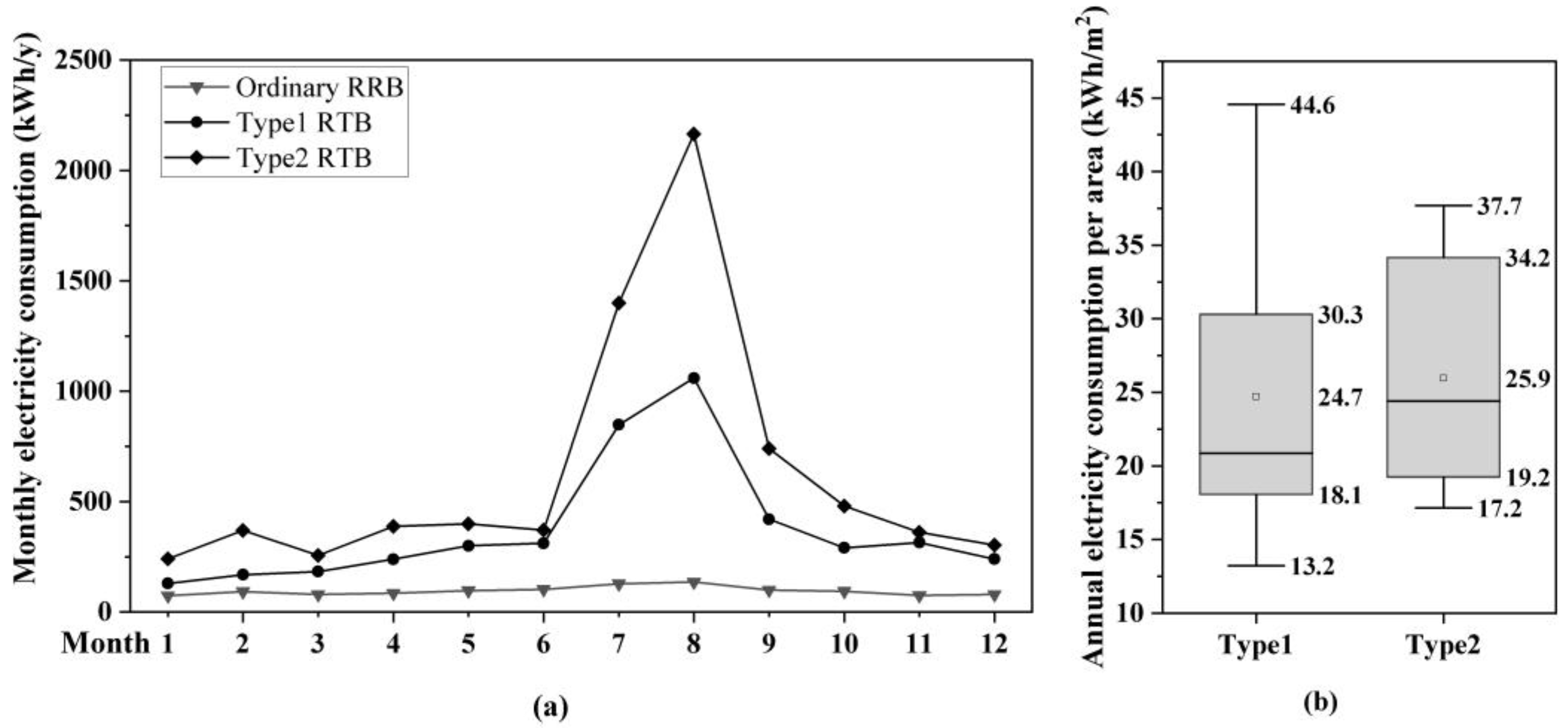
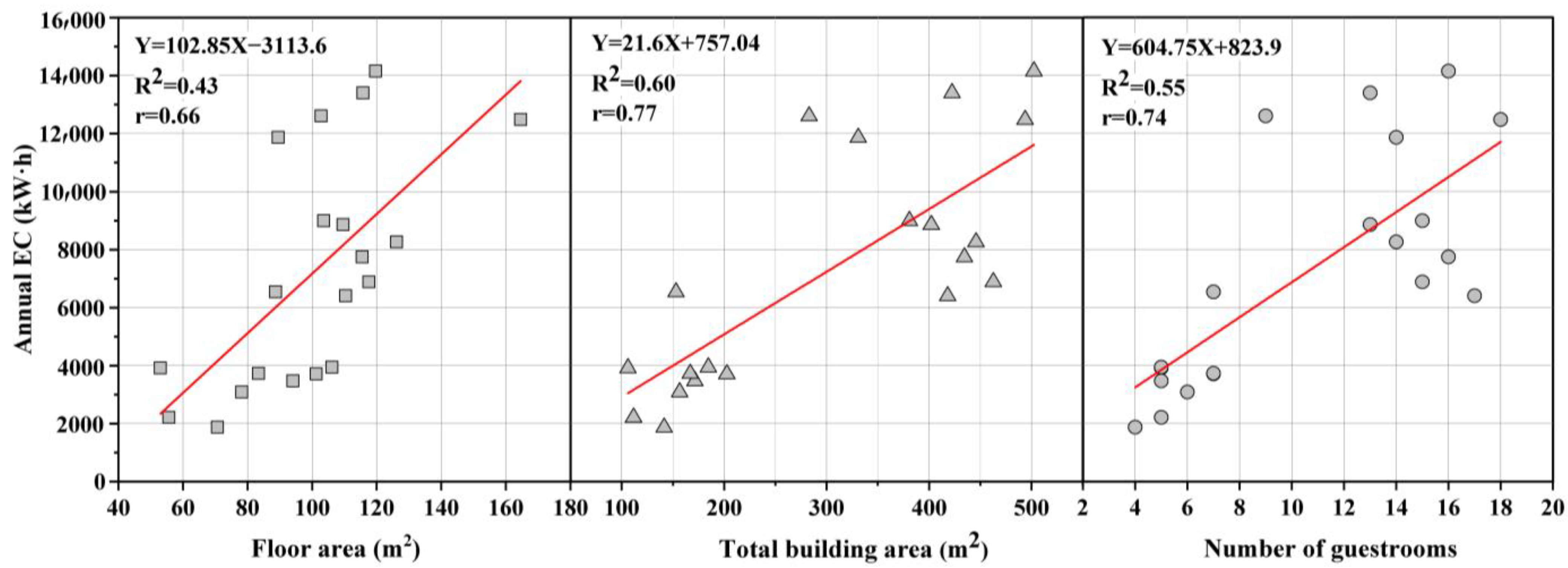
2.1.2. The Characteristics of Energy Consumption in RTBs

The terminal energy consumption of RTBs mostly relies on electricity, except that liquid gas is mostly used for cooking. RT business was greatly impacted by the epidemic. In order to clarify the energy consumption characteristics of RTBs before the epidemic, five consecutive years of the electricity consumption of the surveyed RTBs before 2019 were obtained from the local power sector. At the same time, 10 local ordinary RRBs were randomly selected as a comparison.

As shown in Figure 3a, the electricity consumption of the two types of RTBs was higher than that of ordinary RRBs, especially that of type 2 RTBs. The electricity consumption of local ordinary RTBs was lower due to the small permanent population, even in summer. The fluctuation range of the annual electricity consumption of ordinary RRBs was relatively small. However, the peak–valley fluctuation trend was obvious because of the influence of seasonal characteristics on RT. The RT business in Zhoushan mainly operates from April to October, and from November to March of the next year is the low season. July and August are the peak periods of EC, which are also the hottest months and the peak season of RT in a year. In the peak season of RT, the electricity consumption of RTBs is more than seven times that of ordinary RRBs. Even in quiet periods, the electricity consumption is about 2 to 4 times higher than that of ordinary RRBs due to the return of young and middle-aged labor in rural tourism families to operate RT businesses.

Figure 3a shows that the monthly average electricity consumption of type 2 RTBs was greater than that of type 1 RTBs. However, Figure 3b shows that the annual EC of different RTBs varied significantly. This discrepancy could be attributed to the combined effects of differences in outdoor climate conditions, architectural features, passenger flow, energy management, and energy-saving measures between different RTBs.

A classical statistical analysis was performed to clarify the correlation between EC and the surveyed status of RTBs and to determine the main parameters for building models. Scatter diagrams were drawn, and a simple linear regression analysis was conducted on the correlations between the annual EC and the floor area, total building area, and number of guestrooms. The corresponding equations, R-square values of Pearson correlations (R²), and Pearson correlations (r) are displayed in Figure 4. The results show that the r values between the EC and the floor area, total building area, and number of guest rooms were 0.66, 0.77, and 0.74, respectively, showing a significance level of 0.05 and a strong positive correlation.

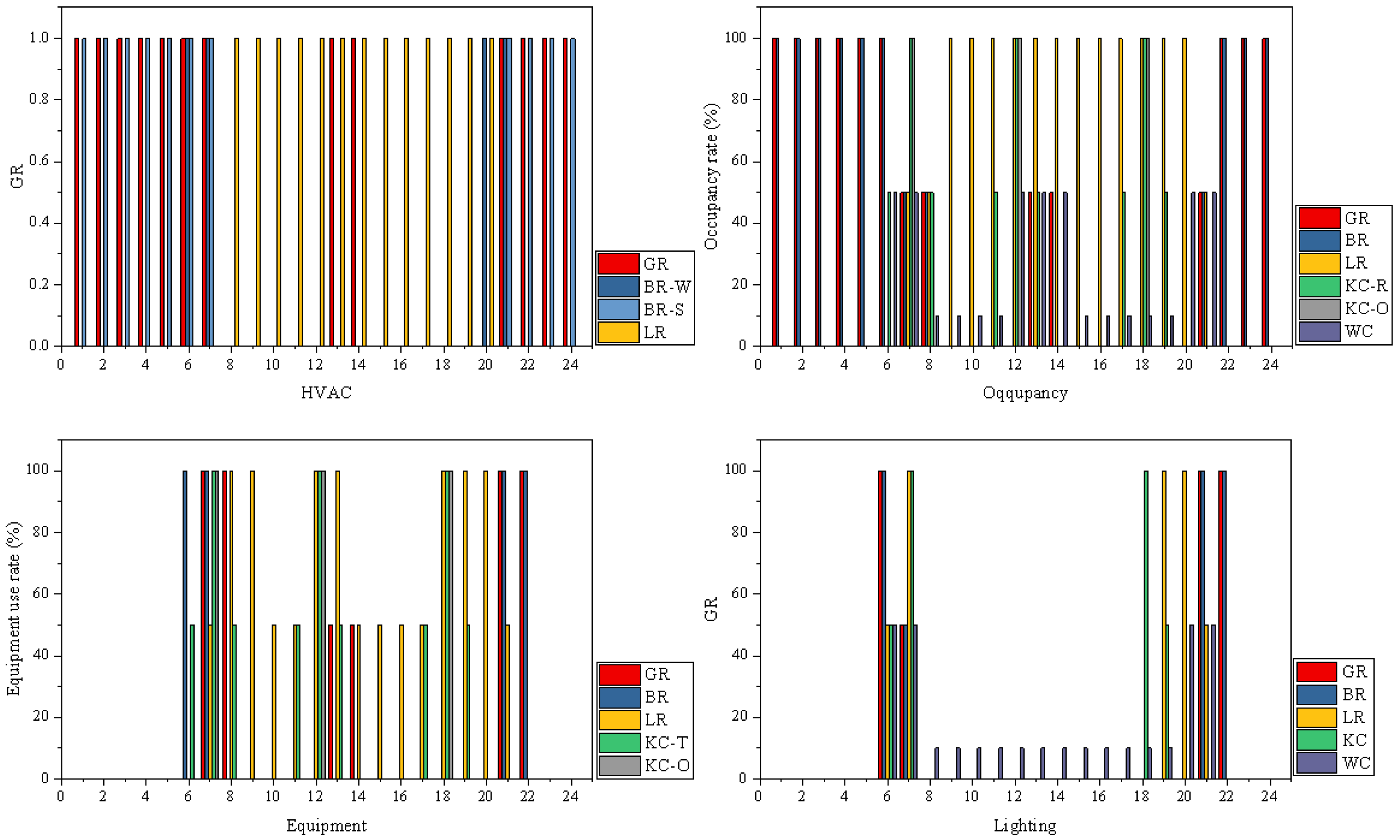
2.1.3. People’s Activities and Equipment Usage in RTBs

The characteristics of people’s activities and equipment usage in RTBs were revealed by a field survey combing device monitoring and interviews. The activities of RT operators and tourists were investigated and recorded in detail, including the daily schedules of people’s activities and the usage of air conditioners, lighting, and other appliances. The energy consumption of air conditioning and the indoor temperature were tested in two typical RTBs to record the air conditioning usage frequency, electricity consumption, and indoor temperature and humidity in 25 guestrooms for three consecutive days using smart meters, and the data were collected at 15-min intervals. The schedules of HVAC operation, occupancy, equipment, and lighting are presented in Figure 5.

2.2. Model Establishment

2.2.1. Benchmark Models

In this section, two RTBs with good fits and patterns typical of the two types of RTBs were selected as the benchmark models for further simulation. Since the floor area, total building area, and number of guestrooms have close relations with EC (Figure 4), the two RTBs had typical plane layouts and all the three parameters were close to the average values. The basic status is listed in

Table 2. Basic information for simulation models.

Content	Type 1	Type 2
Location	Latitude: N 31.17°; Longitude: E 121.43°	Latitude: N 31.17°; Longitude: E 121.43°
Orientation	North and south	North and south
Structure	Stone structure	Brick–concrete structure; thermal bridge: 20%
WWR	South: 25%; North: 20%	South: 30%; North: 25%
External walls	400 mm limestone wall; U = 2.3 W/(m2·K)	240 mm fired perforated brick wall; U = 1.8 W/(m2·K)
External windows	Ordinary aluminum-alloy single-layer glass window; U = 6.0 W/(m2 K); SHGC = 0.75	Ordinary aluminum-alloy single-layer glass window; U = 6.0 W/(m2 ·K); SHGC = 0.75
Roof	Pitched roof (unoccupied): U = 6K W/(m2·K)	Flat roof: U = 3.8 W/(m2·K)
Airtightness	1.0 ach/h	1.0 ach/h

. The plane layouts and the 3D parametric models are displayed in Figure 6.

The benchmark models were established in DesignBuilder (DB), a visual dynamic simulation analysis platform for building energy performance simulation based on EnergyPlus [52]. In the simulation models, the dimensions of the doors and windows were set according to the average WWR value (Figure 2). The building envelopes of RTBs varied for different decorations. In the process of modeling, the envelopes were set according to the common construction. The materials and calculation methods were adopted according to standard [53]. The base values of each parameter for the simulation are listed in

Table 3. Input variables for simulation.

Variables	Units	Base Value	Range	Step	Distribution	Abbr.
Wall U value	W/(m2·K)	2.2	0.4~2.6	0.2	uniform	Wall-U
Windows U value	W/(m2·K)	6.4	1.5~3.5	0.2	uniform	Win-U
Solar heat gain coefficient	-	0.8	0.2~0.8	0.2	uniform	SHGC
Roof U value	W/(m2·K)	3.5/6.0	0.5~6.0	0.2	uniform	Roof-U
External door U value	W/(m2·K)	2.8	2.0~3.0	0.2	uniform	Door-U
Window-to-wall ratio (south)	%	30	20~80	5	uniform	WWR-S
Window-to-wall ratio (north)	%	30	15~80	5	uniform	WWR-N
Shading (south)	m	-	0.3~1.2	0.3	uniform	Shading-S
Shading (east/west)	m	-	0.3~1.2	0.3	uniform	Shading-EW
Infiltration	ach/h	1.0	0.3~1.5	0.2	uniform	Infiltration
Lighting power density	W/(m2)	7	4~8	1	uniform	Lighting
Equipment power density	W/(m2)	15	3~15	2	uniform	Equipment
Occupancy number of people (guest room)	P/room	3	1~4	1	uniform	ONP
Heating set-point temperature	°C	18	16~21	1	uniform	Heating ST
Cooling set-point temperature	°C	26	22~28	1	uniform	Cooling ST

. Additionally, the parameter values and typical daily operating schedules of equipment, lighting, and people’s activities in different thermal zones were established based on relevant standards [21,22] and a field survey (Figure 5).

The parameters of the aspects of the building characteristics, equipment systems, and personnel activity characteristics were set according to relevant standards [21,22], and the threshold range and variation range of each parameter are listed in Table 3. Due to a lack of meteorological files of Zhoushan in the database of DB, the meteorological data of neighboring Shanghai, which are typical for southeastern coastal areas of China, were applied for the simulation. RTBs mainly use split air conditioners for cooling and heating. The field survey revealed that the energy efficiency grade of most air conditioners in RTBs was level 3, while the minimum allowable values of cooling and heating are 3.2 and 2.2, respectively [54]. The best orientation of buildings in Zhejiang Province is from 30° southeast to 15° southwest [55]. In DB, the orientation setting range is from 0° to 360°. Considering the continuity of the data distribution, the range of the orientation was set to 0° to 30°.

The type 1 RTBs were built with local limestone with a thickness of 400 mm. The type 2 RTBs are buildings with brick–concrete structures that were built using 240 mm fired perforated brick. The thermal bridge ratio of type 2 RTBs was set to 20% according to the common practices. In order to determine the proper value of the real infiltration rates of RTBs, the results from Chinese standards [21] were used, combined with the work of Feng et al. [56]. Finally, the building air tightness was set to 1.0 ach/h. The interior loads and temperature settings of the main zones are listed in

Table 4. Interior loads and temperature settings of main zones.

Zone	People (P/room)	Metabolic Rate (W/P)	Temperature (°C)		Lighting (W/m2)	Equipment (W/m2)
			Summer	Winter
Guestroom	3	100	26	18	7	15
Bedroom	2	100	26	18	7	15
Living room	10	110	26	18	7	15
Kitchen	3	160	/	/	7	70
WC	1	120	/	/	7	15

.

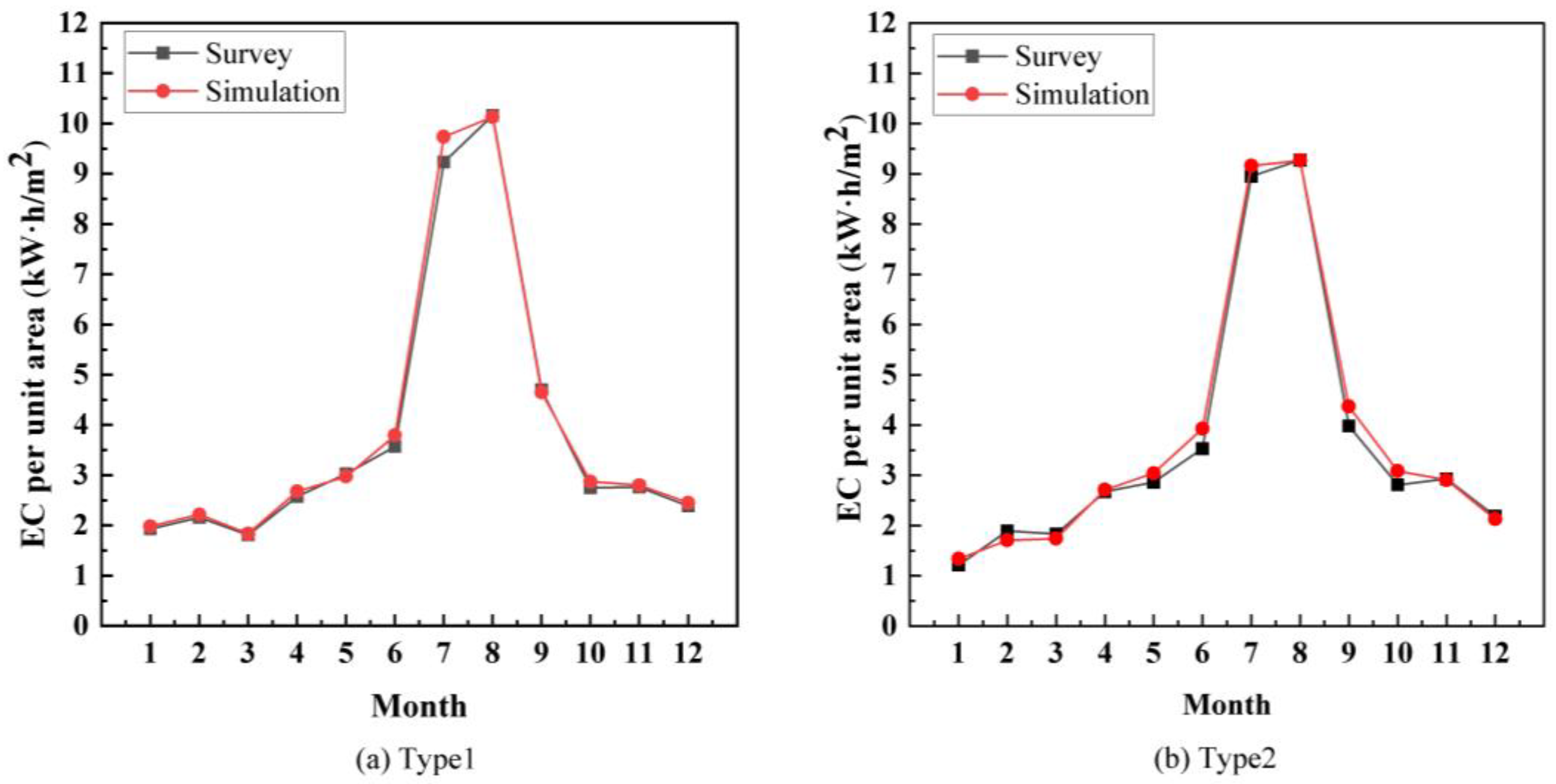
2.2.2. Model Verification and Validation

Due to the uncertainty of the model and parameter settings, there was a large difference between the simulation results of the initial model and the measured values. This difference is known as the energy performance gap [57,58]. Therefore, it was important to verify the model’s accuracy and guarantee the correctness of the simulation and results [59]. Verification and validation were performed before the SA and MOO [60]. Considering the influences of weather, passenger flow, operation, management, and other factors, the energy consumption values were quite different between RTBs. Finally, the monthly EC values of the two types of RTBs with relatively stable passenger flow and operation were selected to verify the benchmark models.

The monthly EC values of type 1 and type 2 RTBs simulated and generated by DB were compared with the surveyed values. First, the monthly EC of lighting and equipment in the spring (March to May) and the autumn seasons (October to November) were compared and adjusted. Then, the occupancy rate and the operation time of air conditioners were adjusted to calibrate the monthly EC in the heating and cooling seasons until the errors were within acceptable tolerances. According to the requirements of Chinese standards [61]; the ASHRAE Guideline (American Society of Heating, Refrigerating and Air-Conditioning Engineers) [62]; and the Federal Energy Management Program (FEMP) Guidelines [63], the accuracy of the model can be verified using normalized mean bias error ($NMBE$), the coefficient of variation of the root-mean-square error ($CvRMSE$), and the coefficient of determination ($R^2$) [57,58]. The smaller the value, the more accurate the model is. The equations are as follows:

$$NMBE=\frac{{\sum }_{i=1}^{12}(E{C}_{M\cdot i}-E{C}_{S\cdot i})}{{\sum }_{i=1}^{12}E{C}_{M·i}}\times 100\%,$$

(1)

$$CvRMSE=\frac{\sqrt{\frac{1}{12}{\sum }_{i=1}^{12}(E{C}_{M·i}-E{C}_{S·i}{)}^2}}{\overline{E{C}_M}}\times 100\%,$$

(2)

$$R^2=1-\frac{{\sum }_{i=1}^{12}(E{C}_{M·i}-E{C}_{S·i}{)}^2}{\overline{{\sum }_{i=1}^{12}(E{C}_{M·i}-\overline{E{C}_M}{)}^2}}\times 100\%,$$

(3)

where $E{C}_{M·i}$ is the measured value of the monthly electricity consumption per area (kWh/m²); $E{C}_{S·i}$ is the simulated value of the monthly electricity consumption per area (kWh/m²); and $\overline{E{C}_M}$ is the average monthly electricity consumption per area (kWh/m²).

The monthly surveyed and simulated EC values, after validation, are displayed in Figure 7. The $CvRMSE$, $NMBE$, and R² values of the type 1 RTBs after verification were 6.97%, −0.26%, and 0.9989, respectively. The $CvRMSE$, $NMBE$, and R² values of type 2 RTBs after verification were 8.24%, −0.75%, and 0.9985, respectively. The results indicate that the reliability of the model was high, but there were still inevitable errors. The possible explanations for the errors are the randomness of the use time, personnel activities, and equipment use of each space; the input value of the EER of the air conditioners; and the power density of the lighting and equipment, which were input according to the rated values rather than the actual values. The reasons for the above errors were basically unavoidable, and the errors in the calibration model were within the acceptable ranges, as shown in

Table 5. Acceptable error ranges.

Index	Chinese Standard [61]	ASHRAE [62]	FEMP [63]
$CvRMSE$	±15	±15	±15
$NMBE$	±15	±5	±5
$R^2$	≥75%

. Therefore, these two models can be used as the benchmark models for SA and MOO.

2.3. Analysis Methods

In this section, three analysis methods are combined and applied to obtain final optimization solutions. After setting the models, key design parameters are determined using an SA. Then, the Pareto front solution sets are obtained through MOO, and the TOPSIS method is used to obtain the optimal solutions from the solution sets. Finally, four evaluation metrics for SA, MOO, and TOPSIS are described.

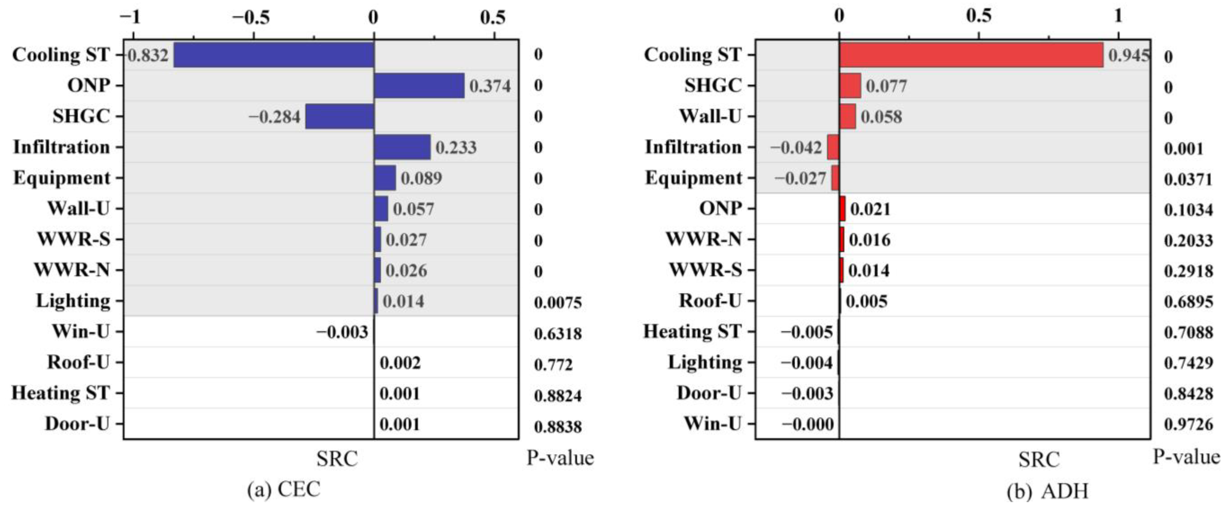
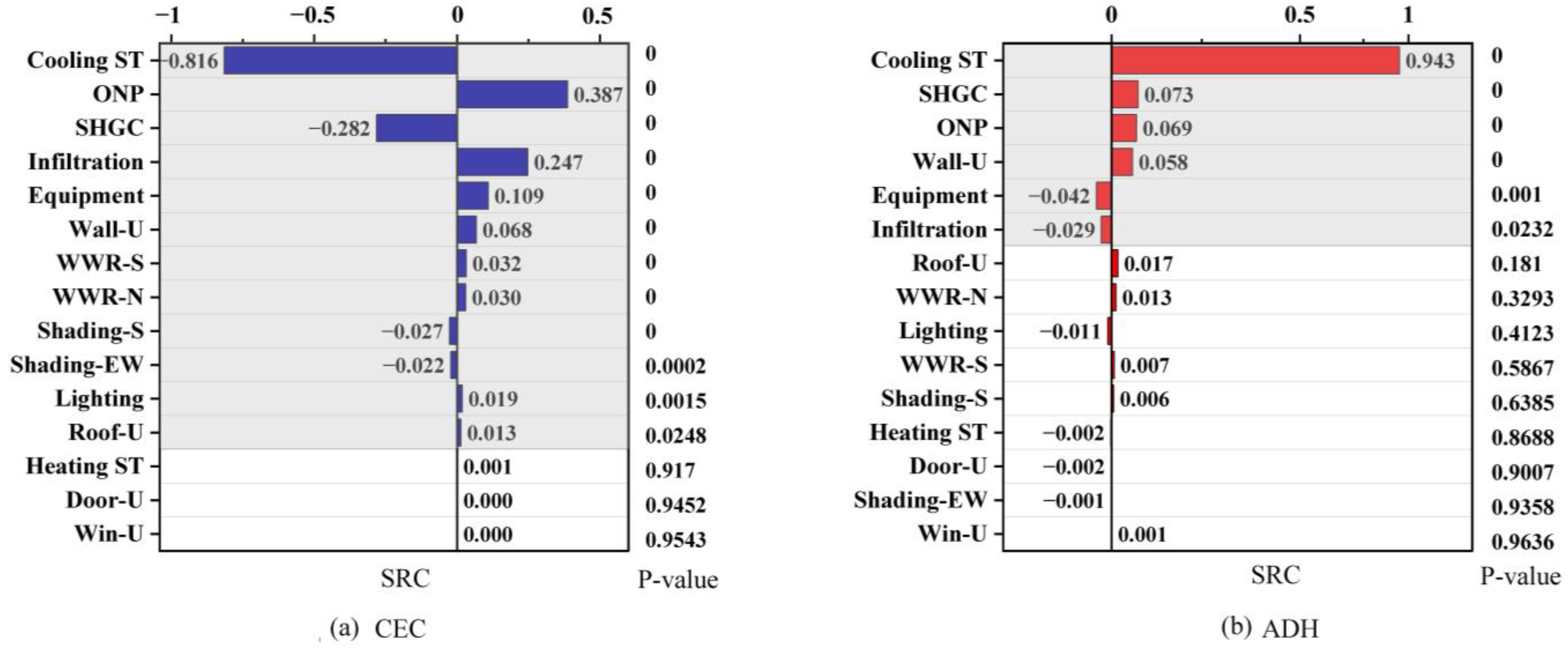
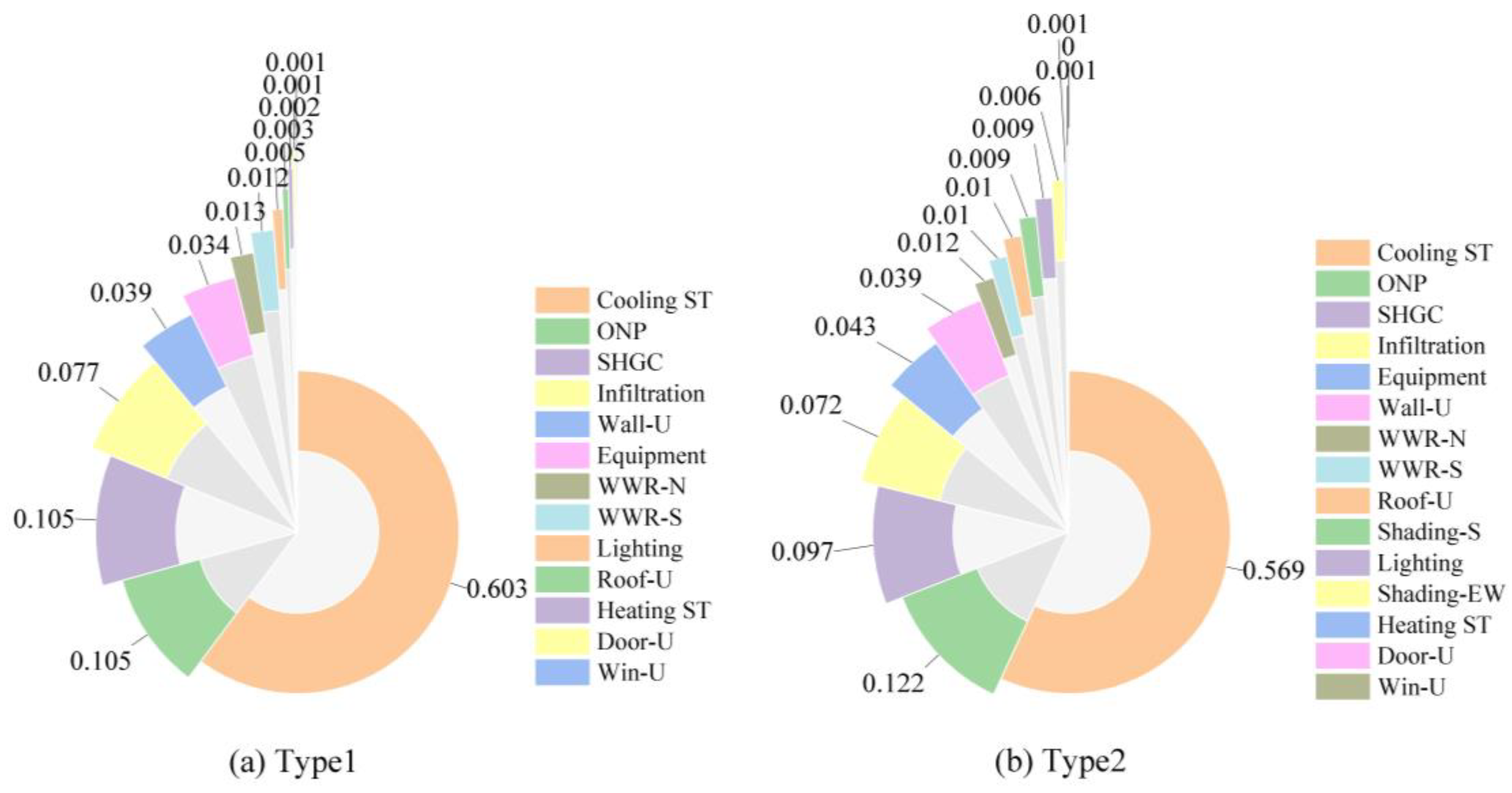
2.3.1. Sensitivity Analysis

The standard regression method, a global SA approach, is adopted to estimate the degree of relative importance among the input variables. The standardized regression coefficient (SRC) outputs the sensitivity of each input variable, thereby identifying the most and least important variables. The magnitude of an SRC value represents the relative influence of the input parameters on the outputs, and the sign represents if the relationship is positive or negative. A larger absolute SRC value indicates that the input parameter plays a more important role in improving the performance [46]. While other regression outputs such as the adjusted R² value and p-value help in determining the level of confidence and reliability of the results, the p-value represents the confidence in the SRC value. If the value of p < 0.05 is considered to be statistically significant, it shows that the SRC value did not occur by chance. In addition, before a global SA, a single-factor sensitivity analysis of each input variable is used to preliminarily judge the degrees of influence and change trends in the outputs. At the same time, the parameter settings for the two RTB models are also checked for errors. One of the most important factors to consider while carrying out an SA is the sampling method. The Sobol sampling method is a quasi-random low-dependency sequence with more space-filling than other methods [26]. The other important factor is the number of runs, which usually determines the size and complexity of the analysis and can even determine the reliability of the results. The minimum population size of the Sobol method is 15. A larger population is selected for a more accurate analysis [50]. Finally, the runs are set to 600 in the simulation.

The input variables are selected according to design measures influencing the thermal and energy performance of RTBs, including the passive design parameters and active design parameters listed in Table 3. The variables are uniformly distributed since all of them are equally probable. Constraints are applied to their ranges according to the national construction codes and standards of China. The cooling electricity consumption (CEC) per area and the annual discomfort hours (ADH) are identified as the objectives in the SA simulation, and they are also objectives for MOO. However, the order and contribution rates of the input variables to the CEC and ADH are different. Then, the comprehensive contribution of each input variable is calculated using the average contribution rate. The detailed steps are as follows:

(1)

SA simulations are carried out, and the matrixes of the SRC values are established:

$$SRC=\begin{array}{c}{D}_1\\ D_2\\ ⋮\\ D_n\end{array}\stackrel{\begin{array}{cccc}{S}_1& S_2& \cdots & S_m\end{array}}{\left[\begin{array}{cccc}{s}_{11}& s_{12}& \cdots & s_{1m}\\ s_{21}& s_{22}& \cdots & s_{2m}\\ ⋮& ⋮& \ddots & ⋮\\ s_{n1}& s_{n2}& \cdots & s_{nm}\end{array}\right]},$$

(4)

where $D_1,D_2,\dots ,D_n$ is the design measures list in Table 3; $n$ is the total number of measures; $n$ = 13 for type 1; $n$ = 15 for type 2; $S_1,S_2,\dots ,S_m$ represent the objectives in the SA$; m$ = 2 is the total number of objectives (CEC and ADH); and $s_{ij}$ is the SRC value of the $i$th design variable to the $m$th objective.

(2)

The contribution rates of the design variables are calculated for each objective, and the contribution rate matrixes ($P=\left\{p_{i·j}\right\}$) are constructed:

$$p_{i·j}=\frac{s_{nm}}{{\sum }_{n=1}^n{s}_{nm}},$$

(5)

(3)

The average contribution rate (ACR) is calculated to obtain the average ACR matrix:

$$ACR=\frac{\left(P_{CEC}+P_{ADH}\right)}{2},$$

(6)

2.3.2. Multi-Objective Optimization

Compared to traditional optimization algorithms such as calculus-based methods and exhaustive methods, a multi-objective genetic algorithm has the advantages of high nonlinearity and robustness and can effectively deal with complex problems that are difficult to solve using traditional optimization algorithms. It has been widely accepted that genetic algorithms are more efficient and accurate than other algorithms in MOO.

DB, as a building energy simulation tool, not only has the advantages of visualization, inter-operability, and reliable results with the integration of EnergyPlus, it also carries an optimization module based on the NSGA-II method, a widely used “fast and elitist multi-objective” genetic algorithm method, and the concepts of the Pareto front and the non-dominated sorting method are also imported [64]. In this work, DB was selected to generate the Pareto-optimal solution sets. In the MOO simulation, a lower mutation rate and a higher crossover rate were set, which were 0.05 and 0.9, respectively, and the population size was set to 1000. The field survey results indicated that the CEC of the RTBs was the largest in summer. Additionally, the RTBs also require higher indoor thermal comfort. Therefore, the CEC per area and the ADH were set as the objectives in the simulation.

2.3.3. TOPSIS Decision-Making Method

In this work, the entropy-based TOPSIS method is applied to make a comprehensive decision, and the optimal scheme is selected from the Pareto solution set. The TOPSIS method is an effective method for solving multi-attribute decision-making problems. In a study conducted by C. L. Hwang and K. Yoon, they proposed the TOPSIS method by ranking alternatives based on the shortest distance from the ideal solution and the farthest distance from the negative ideal solution [65]. The decision result is greatly related to the weight and normalization method. The entropy weight method is a method for objectively determining weights that is frequently used to determine the attribute weights in the TOPSIS method [66]. In addition, min–max normalization (MMN) is the most frequently used method for entropy weight and TOPSIS calculations, according to the research of Chen et al. [67]. Therefore, this method is adopted in this paper. The detailed procedure of the entropy-based TOPSIS method is described as follows:

(1)

The judgment matrix is constructed. Considering the differences in the attributes in units and orders of magnitude, the matrix is normalized using the MMN method. The structure of the normalized matrix can be expressed as follows:

$$Z^{\prime }=\begin{array}{c}{A}_1\\ A_2\\ ⋮\\ A_n\end{array}\stackrel{\begin{array}{cccc}{Z^{\prime }}_1& {Z^{\prime }}_2& \cdots & {Z^{\prime }}_m\end{array}}{\left[\begin{array}{cccc}{Z^{\prime }}_{11}& {Z^{\prime }}_{12}& \cdots & {Z^{\prime }}_{1m}\\ {Z^{\prime }}_{21}& {Z^{\prime }}_{22}& \cdots & {Z^{\prime }}_{2m}\\ ⋮& ⋮& \ddots & ⋮\\ {Z^{\prime }}_{n1}& {Z^{\prime }}_{n2}& \cdots & {Z^{\prime }}_{nm}\end{array}\right]},$$

(7)

where $A_1,A_2,\dots ,A_n$ denote the alternative schemes; ${Z^{\prime }}_1,{Z^{\prime }}_2,\dots ,{Z^{\prime }}_m$ represent the evaluation indexes of the alternative schemes; ${Z^{\prime }}_{ij}$ indicates the performance value of the $j$th index in the $i$th scheme after normalization; $i=\mathrm{1,2},\dots ,n$; and $j=\mathrm{1,2},\dots ,m$.

(2)

The attribute weight ($w_i$) is calculated. The process of determining the weight for the entropy-based TOPSIS method involves establishing a normalized judgment matrix for each evaluation index and calculating the weight of each index based on the entropy value ($E_i$), which can be expressed using the following equation:

$$E_i=-\frac{1}{\mathit{ln}n}{\sum }_{i=1}^n{p}_{ij}\mathit{ln}{p}_{ij},$$

(8)

where $n$ is the number of schemes. $p_{i·j}$ is the contribution rate of a different index that can be calculated according to the following equation:

$$p_{i·j}=\frac{{Z^{\prime }}_{ij}}{{\sum }_{i=1}^n{Z^{\prime }}_{ij}},$$

(9)

Then, the attribute weight ($w_i$) can be calculated using the following equation:

$$w_i=\frac{1-E_i}{{\sum }_{i=1}^n\left(1-E_i\right)},$$

(10)

Finally, the quantitative values can be placed in the above decision matrix.

$$x_{ij}=w_j{z}_{ij},$$

(11)

where $w_j$ is the weight of the $j$th index.

(3)

The positive ideal solution ($x^{+}$) and negative ideal solution ($x^{-}$) are determined using the weighted normalized decision matrix.

$$x^{+}=\left\{x_1^{+},x_2^{+},\dots ,x_m^{+}\right\}=\left\{{max}_{ij}\right\},$$

(12)

$$x^{-}=\left\{x_1^{-},x_2^{-},\dots ,x_m^{-}\right\}=\left\{{min}_{ij}\right\},$$

(13)

(4)

The Euclidean distances from each alternative scheme to the positive ideal solution ($D_i^{+})$ and the negative ideal solution ($D_i^{-}$) are calculated.

$$D_i^{+}=\sqrt{\sum _{j=1}^m{\left(x_{ij}-x_j^{+}\right)}^2}$$

(14)

$$D_i^{-}=\sqrt{\sum _{j=1}^m{\left(x_{ij}-x_j^{-}\right)}^2}$$

(15)

(5)

The relative closeness ($C_i$) of each alternative scheme is calculated, and the preference order is ranked:

$$C_i=\frac{D_i^{-}}{D_i^{-}+D_i^{+}},$$

(16)

where 0 $\le C_i\le 1$. The value of relative closeness ($C_i$) reflects the relative superiority of the alternatives. A larger $C_i$ indicates that the alternative scheme is better, whereas a smaller $C_i$ indicates that the alternative scheme is poorer. The alternative schemes are preference-ranked according to the descending order of the value of $C_i$. The alternative scheme with the maximum $C_i$ value is the best solution.

In this study, the alternative schemes are the Pareto-optimal solutions obtained by the MOO analysis for the two types of RTBs. To evaluate the comprehensive performance of each scheme, in addition to CEC and ADH, the net site energy (NSE) per area and global cost (GC) are also introduced as indexes to evaluate the comprehensive performances of different schemes.

2.3.4. Evaluation Metrics

The CEC is the electricity consumption for cooling in summer. The NSE not only includes cooling consumption but also includes heating, lighting, and equipment in this work. Cooling and heating electricity consumption can be calculated according to the cooling and heating load and the energy efficiency ratio of air conditioners, which is 3.2 in summer and 2.2 in winter (See Section 2.2.1). The ADH is the time when the zone is occupied that the predicted mean vote (PMV) is not in the comfort region (−0.5 ≤ PMV ≤ 0.5), according to ASHRAE 55-2017 [68].

In EPBD (recast) 2010, GC was introduced as an economic evaluation index to assess the energy cost of energy-saving measures for the entire life cycle of buildings. Basinska et al. [69] applied GC to the energy assessment of solutions for the technical equipment of buildings. Ascione et al. [28] and Jie et al. [44] took GC as one of the evaluation criteria of MOO. GC is calculated using the net present value method by calculating the sum of the initial investment costs of energy-saving measures and the discounted annual operating costs during the calculation period without calculating the costs of the main structures of the buildings. The calculation process of GC is shown in the equations below:

$$GC=\frac{C_I+{\sum }_{i=1}^{20}[E_i\times P\times R_d(i\left)\right]}{A},$$

(17)

$$R_d(i)=\frac{1-(1+R_r{)}^{-i}}{R_r},$$

(18)

$$R_r=\frac{R_i-R_e}{1+R_e},$$

(19)

where $GC$ represents the global cost of an RTB during the calculation period per area unit in CNY/m²; $C_I$ is the initial investment cost (CNY); $E_i$ is the energy consumption of year $i$ (kWh); $P$ is the price of electricity in the Zhejiang rural area, which was set at CNY 0.51/kWh $R_d\left(i\right)$ is the discount rate of year $i$; $R_r$ is the real interest rate; $R_e$ is the energy price increase rate, which was set at 1.2%; and $R_i$ is the market interest rate, which was set at 4.0% [26]. Considering the service lives of building components, the operation year ($i$) was set at 20. Furthermore, it was assumed that the building energy consumption and the EC price were unchanged during the calculation period. Local prices collected from market surveys or the official Zhejiang cost information website were used in the calculations. The investment cost of each passive energy-saving measure is given in

Table 6. The initial costs of different passive technical measures.

Envelope	Material	Range	Cost (CNY/m2)
Wall	Inorganic light-weight aggregate insulating mortar	U = 1.0~1.8	25~45
Roof	EPS board	U = 0.4~2.0	10~120
Shading	Concrete shading board	L = 0~1.2 m	60
Window	Ordinary aluminum window (6 mm)	U = 6.0; SHGC=0.75	250
	Ordinary aluminum window (heat-absorbing glass (6 mm))	U = 6.0; SHGC = 0.45	280
	Ordinary aluminum window (6 mm, low-e)	U = 5.3; SHGC = 0.50	350
	Ordinary aluminum window (6 + 12 A + 6 mm)	U = 3.5; SHGC = 0.70	450
	Ordinary aluminum window (6 + 12 A + 6 mm, low-e)	U = 3.0; SHGC = 0.45	550
	Thermal-break aluminum window (6 mm)	U = 5.5; SHGC = 0.75	350
	Thermal-break aluminum window (heat-absorbing glass (6 mm))	U = 5.0; SHGC = 0.45	380
	Thermal-break aluminum window (6 mm, low-e)	U = 4.5; SHGC = 0.50	480
	Thermal-break aluminum window (6 + 12 A + 6 mm)	U = 3.0; SHGC = 0.70	680
	Thermal-break aluminum window (6 + 12 A + 6 mm, low-e)	U = 2.5; SHGC = 0.45	780

The units of U in the range column in this table are W/(m²·K).

.

3. Results and Discussions

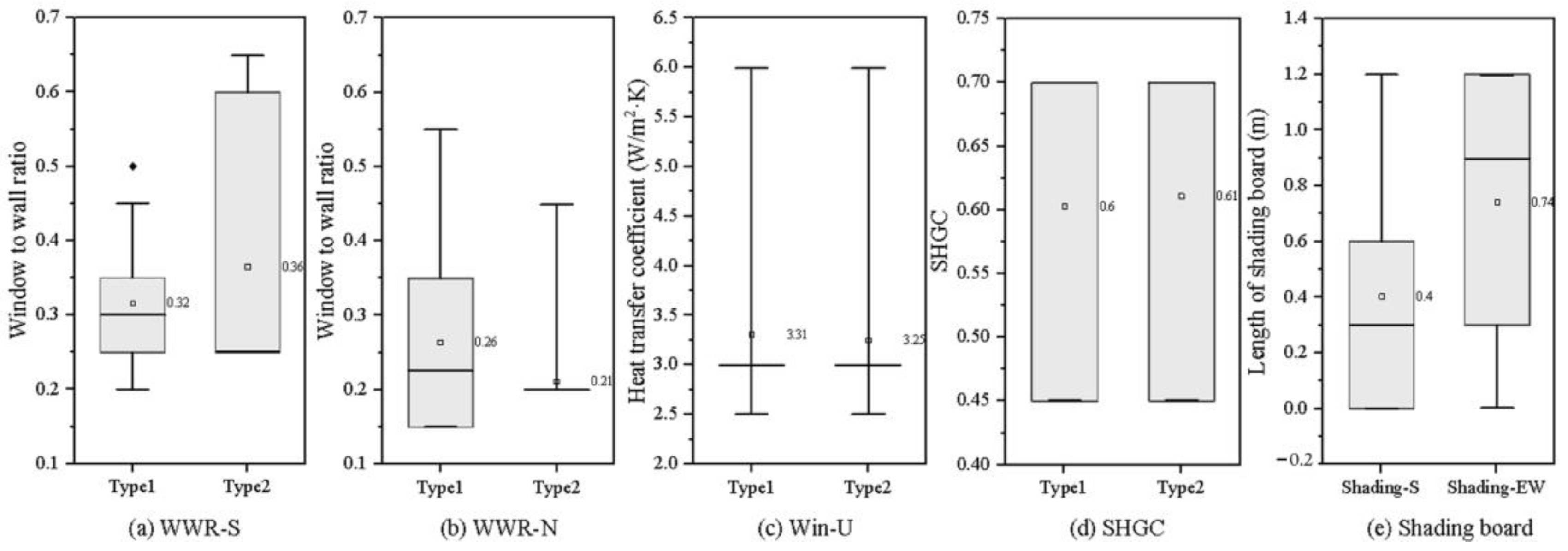
3.1. The Results of the Sensitivity Analysis

In this section, the SAs of the type 1 and type 2 RTBs are analyzed using a standard regression method implemented in DB to calculate the CEC, ADH, and NSE using the Sobol sampling method. The results show that all R² values of the two types of RTBs were greater than 0.900, representing the goodness fit of the complete models and suggesting that most of the key sensitive input variables were identified [70]. It also means that the current results can be considered to identify the most and least sensitive input variables.

Figure 8 and Figure 9 show the SRCs and the corresponding p-values of the influencing variables of the two types of RTBs, respectively. In the figures, the gray areas represent the input variables with P-values less than 0.05; that is, these variables have a great influence on the objectives. Figure 8 shows the order of sensitivity of type 1 RTBs. The factors influencing the CEC with p-values less than 0.05 were the Cooling ST, ONP, SHGC, infiltration, equipment, Wall-U, WWR-S, WWR-N, and lighting. The factors influencing the ADH with p-values less than 0.05 were the Cooling ST, SHGC, Wall-U, infiltration, and equipment. Figure 9 displays the order of sensitivity of the type 2 RTBs. The factors influencing the CEC with p-values less than 0.05 were the Cooling ST, ONP, SHGC, infiltration, equipment, Wall-U, WWR-S, WWR-N, Shading-S, Shading-EW, lighting, and Roof-U. The factors influencing the ADH with p-values less than 0.05 were Cooling ST, SHGC, ONP, Wall-U, equipment, and infiltration.

It can be noted that the SRCs of the input variables for the CEC and ADH are sorted differently, indicating that the sensitivity of different input variables to the output objectives is inconsistent. Furthermore, the applicability of the p-value threshold of 0.05 depends on the modeler’s judgement, as a marginal increase over 0.05 can also be acceptable. For this reason, the comprehensive contribution rates of each input variable for the CEC and ADH were calculated according to the method introduced in Section 2.3.1, and parameters with ACR values greater than 0.005 were selected as sensitivity parameters. The ACR values are shown in Figure 10. The figure shows that the design parameter for RTBs with the highest ACR values was Cooling ST, at 0.603 and 0.569. Other input variables with ACR values greater than 0.005 for type 1 RTBs were ONP, SHGC, infiltration, Wall-U, equipment, lighting, Heating ST, WWR-N, and WWR-S. For type 2 RTBs, the other input variables with ACR values greater than 0.005 were ONP, SHGC, infiltration, equipment, Wall-U, WWR-N, WWR-S, Roof-U, Shading-S, lighting, and Shading-EW. These results seem to suggest that human behavior and equipment factors have greater impacts on the building energy consumption and indoor thermal comfort of RTBs. The main influencing factors related to the building envelope are SHGC, building air tightness, the heat transfer coefficient of the external wall and roof, the window-to-wall area ratio, and the shading setting, but the heat transfer coefficient of outer doors and windows has little effect and can be ignored.

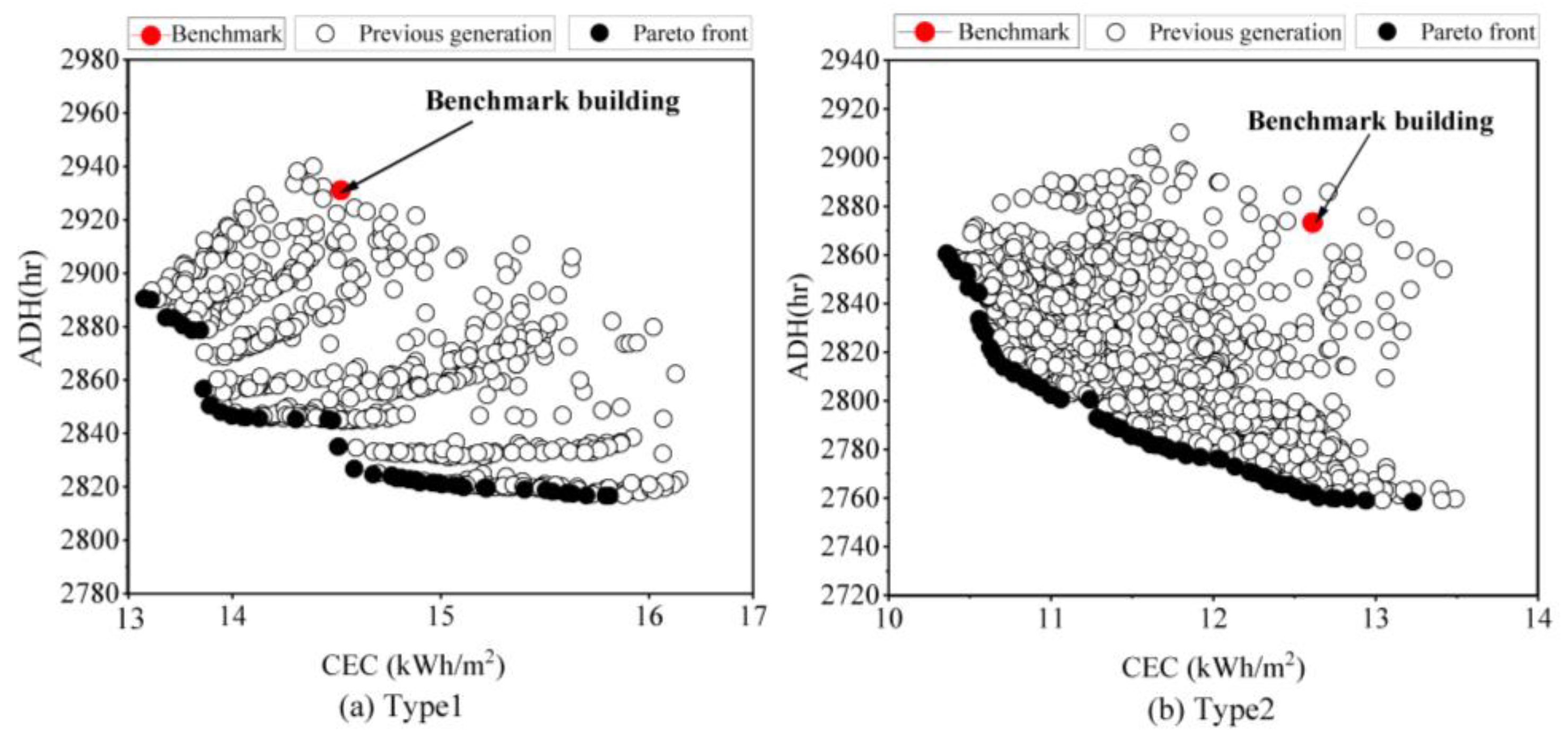
3.2. The Results of Multi-Objective Optimization

Passive energy-saving technology optimization uses the NSGA-II genetic algorithm method in DB for multi-objective screening and optimization. The objectives of MOO are to minimize the ADH and CEC per area. In Section 3.1, the ACR values of the input variables were calculated. Finally, five passive design parameters for type 1 RTBs (SHGC, infiltration, Wall-U, WWR-S, and WWR-N) and eight passive design parameters for type 2 RTBs (SHGC, infiltration, Wall-U, WWR-S, WWR-N, Shading-S, Shading-EW, and Roof-U) with ACR values greater than 0.05 were selected as input parameters for the MOO simulation. According to the standard [43], the air change rate was set to 1 ach/h. The other parameter settings are shown in Table 2. Taking the number of genetic iterations as the constraint, the two types of RTBs were calculated for 500 generations with 20 individuals per generation, a crossing rate of 0.9, and a mutation rate of 0.05. The Pareto front sets of the two types of RTBs were generated, and they are shown in Figure 11. Among the generations, the optimal solutions on the Pareto front surfaces of type 1 and type 2 RTBs were 42 and 70, respectively. It can be seen in Figure 11 that the optimal solution sets of the two types of RTBs were superior to the benchmark buildings in terms of indoor thermal comfort and energy consumption, indicating that passive technology has great potential.

As shown in Figure 11, the CEC per area and ADH of the optimal energy-saving solutions of type 1 and type 2 RTBs were 13.58 kWh/m² and 2890.53 h, and 10.36 kWh/m² and 2860.38 h, respectively, while the values of the optimal comfort solutions of type 1 and type 2 RTBs were 15.82 kWh/m² and 2816.8h, and 13.23 kWh/m² and 2758.40 h, respectively. Comparing the two situations, the optimal energy-saving solutions had lower energy consumption levels, but the comfort was worse. Thus, the CEC per unit area and the ADH for the whole year changed inversely and could not reach their optimal values at the same time.

Figure 12a,b show box graphs of the CEC and ADH of the objectives of the Pareto-optimal solution sets for the two types of RTBs. Furthermore, the NSE and GC of the sets were also simulated and calculated according to the methods in Section 2.3.4 for the TOPSIS analysis. The figure shows that the average CEC per area values of the two RTBs were 14.66 kWh/m² and 11.52 kWh/m², the average ADH values were 2837.92 h and 2794.89 h, the average NSE values were 48.45 kWh/m² and 43.91 kWh/m², and the average GC per area values were CNY 335.49/m² and CNY 292.66/m², respectively. The CEC, GC, ADH, and NSE values of type 2 RTBs were lower than those of type 1 RTBs, indicating that the comprehensive building performance of type 2 RTBs is better than that of type 1 RTBs.

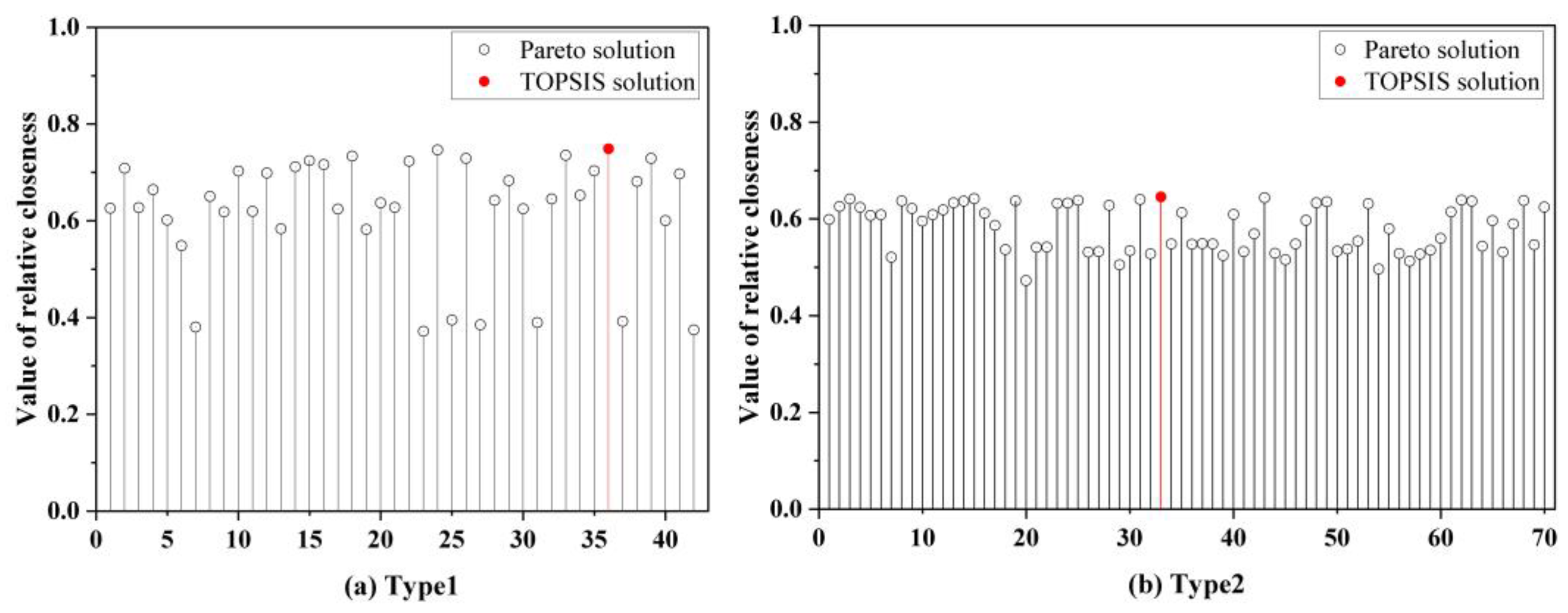
3.3. A Comprehensive Evaluation of TOPSIS

The results in Section 3.2 showed that the optimal solutions of the two types of RTBs were distributed on the Pareto front surface without distinction, but they did not indicate that one optimal solution was better than the other optimal solutions. In this section, an entropy-based TOPSIS decision-making method was used to make further comprehensive decisions to choose the optimal solutions from the Pareto-optimal solution sets. The CEC per area, ADH, GC per area, and NSE per area were the evaluation metrics, and the values were obtained in Section 3.2.

According to the calculation method in Section 2.3.3, the entropy weights of CEC, ADH, NSE, and GC for type 1 RTBs were 0.18, 0.50, 0.10, and 0.21, and for type 2 RTBs they were 0.25, 0.35, 0.11, and 0.29, respectively. The results show that thermal comfort accounted for the highest proportion of the weight. The relative closeness value of each solution was calculated, and they are listed in Figure 13. Figure 13a shows that scheme 36 had the maximum relative closeness value (0.7484). Thus, scheme 15 is the comprehensive optimal solution of type1 RTBs. Similarly, as shown in Figure 13b, the comprehensive optimal solution of type 2 RTBs was scheme 33, with a maximum relative closeness value of 0.6451.

In order to further explain the rationality of the comprehensive optimal solutions, the schemes under different optimal target states were selected from Pareto’s feasible solution sets for analysis and comparison. The best schemes of CEC, ADH, GC, and NSE and the optimal TOPSIS scheme are summarized in

Table 7. The values of different schemes of type 1 and type 2 RTBs.

Type	Schemes	CEC (kWh/m2)	ADH (h)	GC (CNY/m2)	NSE (kWh/m2)	Passive Design Parameters
Type 1	Best CEC/Best NSE/Best GC	13.58	2890.5	225.7	47.56	Wall-U: 1.0W/(m2·K); WWR-S: 20%; WWR-N: 15%; ordinary aluminum window (heat-absorbing glass (6 mm)): U6.0 W/(m2·K), SGHC0.45
	Best ADH	15.82	2816.8	418.3	49.52	Wall-U: 1.0W/(m2·K); WWR-S: 45%; WWR-N: 55%; thermal-break aluminum window (6 + 12 A + 6 mm): U3.0 W/(m2·K), SGHC0.70
	TOPSIS	14.59	2826.8	306.8	48.35	Wall-U: 1.0W/(m2·K); WWR-S: 20%; WWR-N: 15%; thermal-break aluminum window (6 + 12 A + 6 mm): U3.0 W/(m2·K), SGHC0.70
Type 2	Best CEC/Best NSE/Best GC	10.36	2860.4	215.0	42.82	Roof-U: 0.4 W/(m2·K); Wall-U: 1.0W/(m2·K); WWR-S: 25%; WWR-N: 20%; ordinary aluminum window (heat-absorbing glass (6 mm)): U6.0 W/(m2·K), SGHC0.45; Shading-S: 1.2 m; Shading-EW: 1.2 m
	Best ADH	13.23	2758.4	372.9	45.58	Roof-U: 0.4 W/(m2·K); Wall-U: 1.0W/(m2·K); WWR-S: 65%; WWR-N: 45%; thermal-break aluminum window (6 + 12 A + 6 mm): U3.0 W/(m2·K), SGHC0.70; Shading-S: 0 m; Shading-EW: 0 m
	TOPSIS	11.00	2802.3	294.7	43.39	Roof-U: 0.4 W/(m2·K); Wall-U: 1.0W/(m2·K); WWR-S: 25%; WWR-N: 20%; thermal-break aluminum window (6 + 12 A + 6 mm, low-e): U2.5 W/(m2·K), SGHC0.45; Shading-S: 0.3 m; Shading-EW: 0 m

.

Table 7 shows that the best CEC scheme, the best GC scheme, and the best NEC scheme for type 1 RTBs were the same because CEC accounted for a large proportion of NEC in RTBs and GC depended on the adoption of technical measures to reduce CEC. The best ADH scheme had a more comfortable indoor thermal environment than the other schemes, but the CEC, NEC, and GC were higher owing to the reduction in energy consumption, and the improvement in comfort required a certain economic cost. The optimal TOPSIS scheme was the best compromise solution, of which CEC, ADH, GC, and NSE were between the two abovementioned schemes. The situation of the type 2 RTBs was similar to that of the type 1 RTBs. To sum up, the optimal TOPSIS scheme represented the best compromise between energy consumption, economy, and comfort. The best CEC scheme, the best GC scheme, and the best NEC scheme were the optimal solutions for energy conservation and cost, and the best ADH scheme was the solution with the best comfort.

Figure 14 shows the change rates of the CEC, ADH, GC, NSE of each scheme for type 1 and type 2 RTBs relative to the benchmark buildings. Compared to the benchmark buildings, the CEC and NSE of the best energy-saving schemes of type 1 and type 2 RTBs were reduced by 6.53% and 30.71% and by 17.9% and 29.75%, respectively, which proved that these schemes were more energy-efficient than the benchmark buildings. The ADH values of the most comfortable schemes of the two types of RTBs were reduced by 3.90% and 4%, which varied little. The CEC, ADH, and NSE values of the best compromise schemes of type 1 and type 2 RTBs were reduced by 0.44%, 3.55%, and 29.57% and by 12.8%, 2.47%, and 28.81%, respectively. This demonstrates that these three optimal schemes were effective for reducing energy consumption and improving the indoor thermal environment. However, the GC per area values of the three schemes of the two types of RTBs were higher than the benchmark buildings; they increased by 29.56%, 140.09%, and 76.06% and by 40.76%, 144.13%, and 92.96%, respectively. This means that the three types of schemes are uneconomical under the current situation. One reason for this phenomenon is the seasonal characteristic of island tourism, which mainly occurs from June to October. The second reason is the characteristics of the RT operators’ energy-use behaviors. They are accustomed to the lifestyle of districted heating and cooling, and have a higher tolerance for discomfort than urban residents, especially elderly people [71]. In addition, in this study, the impact of a price step on EC was not considered, and the electricity price was considered to be constant. Finally, the design parameters of the different optimal schemes for the two types of RTBs are listed in Table 7.

4. Conclusions

RT has become a new engine to promote the revitalization of rural areas, which means higher requirements for building performance for RTBs. This paper proposes a new methodology for the optimization of the thermal and energy performance of RTBs that combines (1) a field survey to understand the actual status of RTBs in southeastern coastal areas of China; (2) a global SA to keep only the most influential passive design variables; (3) NSGA-II as an optimization solver to identify the Pareto solution sets; and (4) an entropy-based TOPSIS decision method to extract the best compromise solution, the best energy-saving solution, and the best comfort solution. The main results of the study are stated below.

Through the electricity analysis and field investigation of 20 RTBs, it was found that the energy consumption of RTBs presents obvious seasonal characteristics. July and August are the peak season for RT, with the peak period for building energy consumption about five times higher than usual. Based on a detailed field survey using a typology method, two representative types of RTBs in southeastern coastal areas of China were extracted and modeled.

A global SA approach was applied using Sobol sampling methods to analyze the sensitivity factors for the CEC and ADH. In total, 13 input variables for type 1 RTBs and 15 input variables for type 2 RTBs were selected and defined. After the SA analysis, the key passive design parameters of type 1 RTBs were SHGC, infiltration, Wall-U, WWR-S, and WWR-N, and the key passive design parameters of type 2 RTBs were SHGC, infiltration, Wall-U, WWR-S, WWR-N, Shading-S, Shading-EW, and Roof-U.

Based on the NSGA-II algorithm, the MOO approach is carried out as the preliminary optimization of the two types of RTBs. The CEC per area and ADH were set as the optimization objectives of the first stage. In total, 42 Pareto-optimal solutions for type 1 RTBs and 70 Pareto-optimal solutions for type 2 RTBs were generated. Then, an entropy-based TOPSIS decision-making theory was used to find the best compromise solutions from the Pareto-optimal solution sets while comprehensively considering of the performance objectives of CEC, ADH, NSE, and GC. Eventually, the passive design parameters of the best energy-saving scheme (also the best economical solution), the best comfort scheme, and the best compromise scheme were obtained.

However, the types of RTBs were diverse, and the energy-saving measures were varied. This work provides a new method to obtain the optimal solutions of passive measures for two types of RTBs, but the conclusions cannot cover all types. Meanwhile, the SA results show that the active energy-saving measures greatly influence energy consumption. Therefore, more detailed research should be conducted on these problems in the future.

References

1. Shen, S.; Wang, H.; Quan, Q.; Xu, J. Rurality and rural tourism development in China. Tour. Manag. Perspect. 2019, 30, 98–106. [Google Scholar] [CrossRef]
2. Wang, J.; Wu, Z. Annual Report on the Development of Rural Tourism in China (2022); Social Sciences Academic Press: Beijing, China, 2022. [Google Scholar]
3. National Development and Reform Commission; Ministry of Culture and Tourism China. Notice on Publishing the List of the First, Second and Third Batch of National Rural Tourism Key Villages 2019, 2021, 2022. Available online: http://www.gov.cn/zhengce/zhengceku/2021-09/02/content_5634883.htm (accessed on 10 April 2023).
4. Culture and Tourism Market Development. Guidance on the promotion of high-quality development of rural B&B. 2022. Available online: http://www.gov.cn/zhengce/zhengceku/2022-07/19/content_5701748.htm (accessed on 10 April 2023).
5. Peng, S.; Jiang, Y. Roadmap for China’s Building Energy Conservation; China Construction Industry Press: Beijing, China, 2015. [Google Scholar]
6. Li, B.; You, L.; Zheng, M.; Wang, Y.; Wang, Z. Energy consumption pattern and indoor thermal environment of residential building in rural China. Energy Built Environ. 2020, 1, 327–336. [Google Scholar] [CrossRef]
7. Du, Q.; Han, X.; Li, Y.; Li, Z.; Xia, B.; Guo, X. The energy rebound effect of residential buildings: Evidence from urban and rural areas in China. Energy Policy 2021, 153, 112235. [Google Scholar] [CrossRef]
8. Ma, L.; Zhang, X.; Li, D.; Arıcı, M.; Yıldız, Ç.; Li, Q.; Zhang, S.; Jiang, W. Influence of sunspace on energy consumption of rural residential buildings. Sol. Energy 2020, 211, 336–344. [Google Scholar] [CrossRef]
9. Zhu, L.; Wang, B.; Sun, Y. Multi-objective optimization for energy consumption, daylighting and thermal comfort performance of rural tourism buildings in north China. Build. Environ. 2020, 176, 106841. [Google Scholar] [CrossRef]
10. Wang, M.; Huang, S.; Lin, X.; Novianto, D.; Fan, L.; Gao, W.; Wang, Z. Research on Energy Consumption of Traditional Natural Villages in Transition: A Case Study in Zhejiang Province. Energy Power Eng. 2016, 8, 34–50. [Google Scholar] [CrossRef]
11. Tsinghua University Building Energy Conservation Research Center. 2020 Anual Repor on China Building Energy Efficiency; China Architecture& Building Press: Beijing, China, 2020. [Google Scholar]
12. Gong, X.; Chen, C. Field study on summer indoor thermal environment and thermal comfort of rural houses in Hezhou Area. J. Wuhan Univ. 2022, 55, 372–379. [Google Scholar] [CrossRef]
13. Zheng, W.; Bao, L.; Su, S.; Wen, X.; Wang, J. Study on indoor thermal environment of rural residential buildings in Longsheng. J. Shihezi Univ. (Nat. Sci. Ed.) 2019, 37, 720–726. [Google Scholar]
14. Research Center for Building Energy Efficiency, T.U. China Building Energy Efficiency Annual Development Report 2022; Research Center for Building Energy Efficiency: Beijing, China, 2022. [Google Scholar]
15. Zi, C.; Qian, M.; Baozhong, G. The consumption patterns and determining factors of rural household energy: A case study of Henan Province in China. Renew. Sustain. Energy Rev. 2021, 146, 111142. [Google Scholar] [CrossRef]
16. Zou, B.; Luo, B. Rural household energy consumption characteristics and determinants in China. Energy 2019, 182, 814–823. [Google Scholar] [CrossRef]
17. Ran, X.; Geng, S.; Cheng, H.; Tao, S. Changes of Residential Energy Structure and Regional Pollutant Emissions in Rural Areas of Northeast China. Ecol. Environ. Sci. 2022, 1–7. [Google Scholar]
18. LB/T065-2017; Basic requirements and evaluation for homestay inn. Ministry of Housing and Urban-Rural Development of the People’s Republic of China: Beijing, China, 2017.
19. Xi, J.C.; Zhang, M.F.; Ge, Q.S. Evolution of Household Energy Consumption Patterns Induced by Rural Tourism Development and Based on Household Survey Data. J. Nat. Resour. 2011, 26, 981–991. [Google Scholar]
20. Shanghai Municipal Housing and Urban-Rural Development Management Committee. Office Buildings and Large Public Buildings of State Organs in Shanghai in 2020 Energy Consumption Monitoring and Analysis Report; Shanghai Municipal Housing and Urban-Rural Development Management Committee: Shanghai, China, 2021. [Google Scholar]
21. GB/T 50824-2013; Design standard for energy efficiency of rural residential buildings. Ministry of Housing and Urban-Rural Development of the People’s Republic of China: Beijing, China, 2013.
22. GB 55015-2021; General code for energy efficiency and renewable energy application in buildings. Ministry of Housing and Urban-Rural Development of the People’s Republic of China: Beijing, China, 2021.
23. Fan, Z.; Liu, M.; Tang, S. A multi-objective optimization design method for gymnasium facade shading ratio integrating energy load and daylight comfort. Build. Environ. 2022, 207, 108527. [Google Scholar] [CrossRef]
24. Wang, Y.; Yang, W.; Wang, Q. Multi-objective parametric optimization of the composite external shading for the classroom based on lighting, energy consumption, and visual comfort. Energy Build. 2022, 275, 112441. [Google Scholar] [CrossRef]
25. Sha, H.; Xu, P.; Yan, C.; Ji, Y.; Zhou, K.; Chen, F. Development of a key-variable-based parallel HVAC energy predictive model. Build. Simul. 2022, 15, 1193–1208. [Google Scholar] [CrossRef]
26. Chen, R.; Tsay, Y.-S.; Ni, S. An integrated framework for multi-objective optimization of building performance: Carbon emissions, thermal comfort, and global cost. J. Clean. Prod. 2022, 359, 131978. [Google Scholar] [CrossRef]
27. Ciardiello, A.; Rosso, F.; Dell’Olmo, J.; Ciancio, V.; Ferrero, M.; Salata, F. Multi-objective approach to the optimization of shape and envelope in building energy design. Appl. Energy 2020, 280, 115984. [Google Scholar] [CrossRef]
28. Ascione, F.; Bianco, N.; Mauro, G.M.; Napolitano, D.F. Building envelope design: Multi-objective optimization to minimize energy consumption, global cost and thermal discomfort. Application to different Italian climatic zones. Energy 2019, 174, 359–374. [Google Scholar] [CrossRef]
29. Abdou, N.; EL Mghouchi, Y.; Hamdaoui, S.; EL Asri, N.; Mouqallid, M. Multi-objective optimization of passive energy efficiency measures for net-zero energy building in Morocco. Build. Environ. 2021, 204, 108141. [Google Scholar] [CrossRef]
30. Palonen, M.O.; Hamdy, M.; Hasan, A. Mobo A New Software For Multi-objective Building Performance Optimization. In Proceedings of the 13th Internationcal Conference of the IBPSA; IBPSA c/o Miller-Thompson: Toronto, ON, Canada, 2013; Volume 13, pp. 2567–2574. [Google Scholar] [CrossRef]
31. Ebrahimi-Moghadam, A.; Ildarabadi, P.; Aliakbari, K.; Fadaee, F. Sensitivity analysis and multi-objective optimization of energy consumption and thermal comfort by using interior light shelves in residential buildings. Renew. Energy 2020, 159, 736–755. [Google Scholar] [CrossRef]
32. Baghoolizadeh, M.; Rostamzadeh-Renani, M.; Dehkordi, S.A.H.H.; Rostamzadeh-Renani, R.; Toghraie, D. A prediction model for CO2 concentration and multi-objective optimization of CO2 concentration and annual electricity consumption cost in residential buildings using ANN and GA. J. Clean. Prod. 2022, 379, 134753. [Google Scholar] [CrossRef]
33. Mostafazadeh, F.; Eirdmousa, S.J.; Tavakolan, M. Energy, economic and comfort optimization of building retrofits considering climate change: A simulation-based NSGA-III approach. Energy Build. 2023, 280, 112721. [Google Scholar] [CrossRef]
34. Luo, Z.; Lu, Y.; Cang, Y.; Yang, L. Study on dual-objective optimization method of life cycle energy consumption and economy of office building based on HypE genetic algorithm. Energy Build. 2022, 256, 111749. [Google Scholar] [CrossRef]
35. Xu, Y.; Zhang, G.; Yan, C.; Wang, G.; Jiang, Y.; Zhao, K. A two-stage multi-objective optimization method for envelope and energy generation systems of primary and secondary school teaching buildings in China. Build. Environ. 2021, 204, 108142. [Google Scholar] [CrossRef]
36. Zhang, X.; Zhang, X. Comparison and sensitivity analysis of embodied carbon emissions and costs associated with rural house construction in China to identify sustainable structural forms. J. Clean. Prod. 2021, 293, 126190. [Google Scholar] [CrossRef]
37. Li, H.; Wang, S.; Cheung, H. Sensitivity analysis of design parameters and optimal design for zero/low energy buildings in subtropical regions. Appl. Energy 2018, 228, 1280–1291. [Google Scholar] [CrossRef]
38. Yip, S.; Athienitis, A.K.; Lee, B. Early stage design for an institutional net zero energy archetype building. Part 1: Methodology, form and sensitivity analysis. Sol. Energy 2021, 224, 516–530. [Google Scholar] [CrossRef]
39. Yongjun, S. Sensitivity analysis of macro-parameters in the system design of net zero energy building. Energy Build. 2015, 86, 464–477. [Google Scholar] [CrossRef]
40. Rasouli, M.; Ge, G.; Simonson, C.J.; Besant, R.W. Uncertainties in energy and economic performance of HVAC systems and energy recovery ventilators due to uncertainties in building and HVAC parameters. Appl. Therm. Eng. 2013, 50, 732–742. [Google Scholar] [CrossRef]
41. Li, H.; Wang, S.; Cheung, H.; Dominique, M.; Marcello, C.; Frédéric, H. A comparison of methods for uncertainty and sensitivity analysis applied to the energy performance of new commercial buildings. Energy Build. 2018, 166, 489–504. [Google Scholar] [CrossRef]
42. Hsu-Shih, S.; Shyur, H.-L.; Stanley Lee, E. An extension of TOPSIS for group decision making. Math. Comput. Model. 2007, 45, 801–813. [Google Scholar] [CrossRef]
43. Pang, Z.; O’Neill, Z.; Li, Y.; Niu, F. The role of sensitivity analysis in the building performance analysis: A critical review. Energy Build. 2020, 209, 109659. [Google Scholar] [CrossRef]
44. Jie, P.; Zhang, F.; Fang, Z.; Wang, H.; Zhao, Y. Optimizing the insulation thickness of walls and roofs of existing buildings based on primary energy consumption, global cost and pollutant emissions. Energy 2018, 159, 1132–1147. [Google Scholar] [CrossRef]
45. Tian, W. A review of sensitivity analysis methods in building energy analysis. Renew. Sustain. Energy Rev. 2013, 20, 411–419. [Google Scholar] [CrossRef]
46. Zhang, Y.; Zhang, X.; Huang, P.; Sun, Y. Global sensitivity analysis for key parameters identification of net-zero energy buildings for grid interaction optimization. Appl. Energy 2020, 279, 115820. [Google Scholar] [CrossRef]
47. Bre, F.; Silva, A.S.; Ghisi, E.; Fachinotti, V.D. Residential building design optimisation using sensitivity analysis and genetic algorithm. Energy Build. 2016, 133, 853–866. [Google Scholar] [CrossRef]
48. Tushar, Q.; Bhuiyan, M.; Sandanayake, M.; Zhang, G. Optimizing the energy consumption in a residential building at different climate zones: Towards sustainable decision making. J. Clean. Prod. 2019, 233, 634–649. [Google Scholar] [CrossRef]
49. Maučec, D.; Premrov, M.; Leskovar, V. Use of sensitivity analysis for a determination of dominant design parameters affecting energy efficiency of timber buildings in different climates. Energy Sustain. Dev. 2021, 63, 86–102. [Google Scholar] [CrossRef]
50. Naji, S.; Aye, L.; Noguchi, M. Sensitivity analysis on energy performance, thermal and visual discomfort of a prefabricated house in six climate zones in Australia. Appl. Energy 2021, 298, 117200. [Google Scholar] [CrossRef]
51. Koen, C.V.S. Modelling domestic energy consumption at district scale: A tool to support national and local energy policies. Environ. Model. Softw. 2011, 26, 1186–1198. [Google Scholar] [CrossRef]
52. Shen, Y.; Pan, Y. BIM-supported automatic energy performance analysis for green building design using explainable machine learning and multi-objective optimization. Appl. Energy 2023, 333, 120575. [Google Scholar] [CrossRef]
53. GB 50176-2016; Code for Thermal Design of Civil Building. Ministry of Housing and Urban-Rural Development of the People’s Republic of China: Beijing, China, 2016.
54. GB 12021.3-2004; Minimum Allowable Values of the Energy Efficiency and Energy Efficiency Grades for Room Air Conditioners. National Standardization Management Committee: Beijing, China, 2010.
55. DB33/1015-2021; Design Standard for Energy Efficiency of Residential Buildings. Department of Housing and Urban-Rural Development of Zhejiang Province: Hangzhou, China, 2021.
56. Feng, X.; Yan, D.; Peng, C.; Jiang, Y. Analysis of the impact of building airtightness on residential energy consumption. HV AC 2014, 44, 372–380. [Google Scholar]
57. Pachano, J.E.; Bandera, C.F. Multi-step building energy model calibration process based on measured data. Energy Build. 2021, 252, 111380. [Google Scholar] [CrossRef]
58. Pan, Y.; Ying, Y. Building Performance Gap and Building Energy Model Calibration. J. BEE 2021, 49, 370. [Google Scholar]
59. Zuhaib, S.; Hajdukiewicz, M.; Goggins, J. Application of a staged automated calibration methodology to a partially-retrofitted university building energy model. J. Build. Eng. 2019, 26, 100866. [Google Scholar] [CrossRef]
60. Kleijnen, J.P.C. Verification and validation of simulation models. Eur. J. Oper. Res. 1995, 82, 145–162. [Google Scholar] [CrossRef]
61. JGJ 176-2009; Technical Code for the Retrofitting of Public Building on Energy Efficiency. Ministry of Housing and Urban-Rural Development of the People’s Republic of China: Beijing, China, 2019.
62. ASHRAE Guideline, Guideline 14-2002, Measurement of Energy and Demand Savings; American Society of Heating, Ventilating, and Air Conditioning Engineers: Atlanta, GA, USA, 2002.
63. M&V Guidelines: Measurement and Verification for Performance-Based Contracts, Version 4.0; Federal Energy Management Program: New York, NY, USA, 2015.
64. Deb, K.; Pratap, A.; Agarwal, S.; Meyarivan, T.A.M.T. A fast and elitist multi-objective genetic algorithm: NSGA-II. IEEE Trans. Evol. Comput. 2002, 6, 181–197. [Google Scholar] [CrossRef]
65. Yoon, K.P.; Hwang, C.L. Multiple Attribute Decision Making; Springer-Verlag: Berlin/Heidelberg, Germany, 1981. [Google Scholar]
66. Li, H.; Huang, J.; Hu, Y.; Wang, S.; Liu, J.; Yang, L. A new TMY generation method based on the entropy-based TOPSIS theory for different climatic zones in China. Energy 2021, 231, 120723. [Google Scholar] [CrossRef]
67. Chen, P. Effects of normalization on the entropy-based TOPSIS method. Expert Syst. Appl. 2019, 136, 33–41. [Google Scholar] [CrossRef]
68. ASHRAE Standard 55-2017; Thermal Envrionmental Conditons for Human Occupancy. ASHRAE: Peachtree Corners, GA, USA, 2017.
69. Basinska, M.; Koczyk, H.; Szczechowiak, E. Sensitivity analysis in determining the optimum energy for residential buildings in Polish conditions. Energy Build. 2015, 107, 307–318. [Google Scholar] [CrossRef]
70. Saltelli, A.; Ratto, M.; Andres, T.; Campolongo, F.; Cariboni, J.; Gatelli, D.; Saisana, M.; Tarantola, S. Global Sensitivity Analysis: The Primer; John Wiley & Sons: Hoboken, NJ, USA, 2008. [Google Scholar]
71. Yang, Z.; Zhang, W.; Qin, M.; Liu, H. Comparative study of indoor thermal environment and human thermal comfort in residential buildings among cities, towns, and rural areas in arid regions of China. Energy Build. 2022, 273, 112373. [Google Scholar] [CrossRef]
Figure 1. Research framework.
Sustainability 15 07238 g001
Figure 2. Building characteristics of different RTB types: (a) building area; (b) number of guestrooms; (c) WWR; (d) orientation.
Sustainability 15 07238 g002
Figure 3. Comparison of EC of three different types of buildings: (a) monthly EC of ordinary RRBs, type 1 RTBs, and type 2 RTBs; (b) annual EC per area of type 1 and type 2 RTBs.
Sustainability 15 07238 g003
Figure 4. Correlation between annual EC and floor area, total building area, and number of guestrooms.
Sustainability 15 07238 g004
Figure 5. Schedules of HVAC operation, occupancy, equipment, and lighting.
Sustainability 15 07238 g005
Figure 6. Plane layouts and 3D models of type 1 and type 2 RTBs.
Sustainability 15 07238 g006
Figure 7. Monthly EC (surveyed values and simulated values).
Sustainability 15 07238 g007
Figure 8. SRCs and p-values of type 1 RTBs.
Sustainability 15 07238 g008
Figure 9. SRCs and p-values of type 2 RTBs.
Sustainability 15 07238 g009
Figure 10. Contribution rate of each input variable of type 1 and type 2 RTBs.
Sustainability 15 07238 g010
Figure 11. Pareto front generations and previous generations of the two types of RTBs.
Sustainability 15 07238 g011
Figure 12. Pareto-optimal solution sets of the two types of RTBs.
Sustainability 15 07238 g012
Figure 13. Relative closeness values of schemes of type 1 and type 2 RTBs.
Sustainability 15 07238 g013
Figure 14. Change rates of CEC, ADH, GC, and NSE of each scheme relative to the benchmark buildings.
Sustainability 15 07238 g014