AI-Based Degradation Index from the Microstructure Image and Life Prediction Models Based on Bayesian Inference

Abstract

In this study, we propose a consistent and explainable degradation indexing method and a non-destructive-based degradation and creep-life prediction method from extensive destructive test (creep-rupture) data of a nickel-based superalloy (DA-5161 SX), an extreme-environment material. High-temperature components made of nickel-based superalloys that operate in extreme environments (e.g., gas turbine blades) deteriorate over time and shorten the life of the device. To ensure the safety and efficiency of the equipment, it is important to predict the lifetime of high-temperature parts, and a consistent and explanatory degradation index and a reliable predictive model that can predict the degree of degradation and life without destructive testing of high-temperature parts are needed. As the degradation of nickel-based superalloys progresses, degradation indices reflecting the geometrical characteristics are required that focus on the fact that the shape of the gamma-prime phase becomes longer and larger. A representative value of the degradation index was selected through parameter inference based on a Bayesian method, and the high-dimensional degradation index of previous studies was simplified to only one dimension. The robustness of the degradation index quantification model was verified by confirming that the degradation index obtained from 20% of the test images had the lowest change rate of the degradation index obtained from 80% of the training images at 6.9%. The basis for predicting the life of high-temperature parts without destructive testing was established in the degradation index and life prediction model by connecting environmental conditions and degradation indices/the LMP (Larson–Miller parameter) to represent creep life in regression models. Gaussian process regression (GPR) models based on sampling-based Bayesian inference performed well in terms of both RMSE in the degradation index and the LMP prediction model, demonstrating robust behavior in performance variation. This may be used as a key health factor that indicates the soundness of diagnostic solutions in the future, and it is expected to be a foundational technology for decision-making models for maintenance, repair, and disposal.

1. Introduction

1.1. Background

The development of artificial intelligence technologies such as machine learning and deep learning is accelerating due to the combination of vast amounts of data and abundant computing resources such as big data platforms. In recent years, the Bayesian approach has become easier for the analysis of medium or small data as well as big data due to advanced computing technology. It is difficult to make decisions with little data because of uncertainty. The Bayesian approach quantifies uncertainty as a probability and provides an intuitive explanation by inferring the posterior distribution of unknown parameters based on available evidence, making it suitable for decision making [1].

In manufacturing, prognostic health management (PHM) is a key element that can overcome the limitations of traditional reliability analysis. PHM focuses on using device sensor signals to monitor device health, detect outliers, diagnose faults, and most importantly, predict remaining useful life (RUL). This has strong economic benefits for the owners of the equipment. The PHM-based maintenance strategy predicts when a device failure will occur and maintains the machine normally, unlike the conventional maintenance strategy that is initiated when a failure occurs or relies on scheduled maintenance over time [2].

Efforts to improve the environment, such as national energy security and the National Determined Contribution (NDC), are becoming more important internationally, and many strategies focus on the infrastructure industry, especially the power generation industry.

Table 1. Power supply composition forecast by year in the Republic of Korea [3]. “Reprinted/adapted with permission from Ref. [3]. 2020, Ministry of Trade, Industry and Energy, Korea Open Government License(KOGL) Type 1.”.

Year	Description	Coal	LNG
2020	Capacity (GW)	35.3	41.3
	Weight (%)	31.9	37.4
2022	Capacity (GW)	37.8	43.3
	Weight (%)	32.0	36.7
2030	Capacity (GW)	31.9	55.5
	Weight (%)	26.1	45.3
2034	Capacity (GW)	28.3	59.1
	Weight (%)	22.7	47.3

shows the composition of power sources by year in Korea’s ninth basic electricity supply and demand plan. The main power sources are nuclear power, coal, and LNG power. Compared to 2020, the proportion of coal power generation in the 2034 target plan decreases (31.9% → 22.7%). The proportion of LNG power generation increases significantly (37.4% → 47.3%) [3]. According to this trend, the demand for gas turbines is expected to increase. Thus, gas turbines are essential to ensure national competitiveness, and the importance of performance, efficiency, safety, and environmental impact is expected to increase. As shown in Figure 1, Doosan Enerbility developed Korea’s first gas turbine model (DGT6-300H S1). In addition, R&D for eco-friendly and high-performance energy production such as hydrogen hybrid combustion turbines, hydrogen turbines, and ammonia turbines are being conducted in cooperation between public and private sectors.

Industrial gas turbine engines, which play a key role in solving energy and environmental problems, consist of four main components: a compressor, a combustor, a turbine, and a generator. More thermal efficiency can be achieved by increasing the turbine inlet temperature (TIT). The latest and most advanced Grade J gas turbines reach turbine inlet temperatures of up to 1600 °C and efficiencies up to 61.5%. For high-temperature components such as turbine blades, vanes, and combustors, it is necessary to select an appropriate material that can withstand harsh conditions. In particular, the maximum energy is generated by the turbine blades from high-temperature and high-pressure gas. So, the turbine blades are exposed to high temperature and high pressure, causing fatigue, creep, erosion, corrosion, and overheating. Blades can break due to high vibration and resonance. In fact, 42% of gas turbine failures are due to turbine blade failure. The most important aspect of turbine blades’ lifespan is high creep resistance at higher temperatures [5,6].

Because of its excellent properties, nickel is widely used in manufacturing, such as making superalloys with superheat resistance or making Ti-Ni-Ti sandwich structures for 3D printing [7]. The first stage of the turbine blade must be able to withstand very high temperatures, so a nickel-based superalloy with excellent mechanical properties is often used. Single-crystal nickel-based superalloys are strengthened by a secondary phase called the gamma-prime phase, and the mechanical properties at high temperatures depend on the shape, size, and distribution of the microstructure. The microstructure of the turbine blade is degraded during operation, including rafting, coarsening, and concrescence of the gamma prime, as shown in Figure 2. This influences mechanical fatigue properties and tensile properties under heat and creep and reduces the fatigue resistance. For this reason, efforts have been made to find an appropriate quantifiable characteristic indicator of a consistent microstructure on gamma/gamma prime for nickel-based superalloys. However, researchers have focused on developing physical models for establishing quantitative relationships between the states of microstructures, aging or service processes, and the corresponding phases of physical properties. A data-driven model for small data can be an alternative to developing quantitative relationships beyond the conventional method [8].

The gas path analysis (GPA) method is traditionally used for gas turbine diagnosis. This is a method of calculating component characteristic parameters such as compressor and turbine efficiency, heat of combustion of fuel, and unmeasured values of gas path temperature and pressure from measured data [9]. GPA is also a method of providing early warning information so that defects or vibrations in gas turbines do not become worse. GPA is based on thermodynamic model decision making and data-driven artificial intelligence. The health parameters of major components belonging to the gas path indicate the health status of the gas turbine, such as the characteristic index of the gas turbine compressor and turbine flow rate, the operating efficiency, and the combustor efficiency characteristic index [10]. Currently, various artificial intelligence models and optimization methods such as neural networks, Bayesian belief networks, and genetic algorithms are being used to diagnose the health status of gas turbines [11].

Accurate diagnosis of the condition of heavy equipment materials used in extreme environments increases equipment efficiency and predicts the appropriate maintenance time to reduce operating and maintenance costs and reduces the risk of accidents due to damage. A turbine blade is a key component of a gas turbine operating in an extreme environment. In the current material degradation evaluation method, the microstructure of the cut surface is obtained by destroying high-temperature parts and then using an imaging device such as a scanning electron microscope (SEM). An image of the microstructure of the material can be obtained even when a replica is extracted for repair of a component in operation. Creep life and residual life can be calculated through the life fraction rule, where the Larson–Miller parameter (LMP) is used to extrapolate the results of the stress-rupture test to the actual operating conditions; the LMP is also a major parameter in predicting the creep life [12]. LMP can be obtained by inputting the rupture time and temperature obtained in the creep test as follows [13]:

$$\mathrm{LMP}=\mathrm{T}\left(\mathrm{C}+\log \mathrm{t}\right),$$

(1)

where T is the Kelvin temperature, t is the stress-rupture time, and C is a constant, usually 20.

1.2. Related Works

Feature engineering is the process of converting features of raw data into numerical values. Proper features are a major step in data preprocessing that can improve the quality of prediction results while simplifying machine learning models. Feature engineering methods can be largely divided into three categories: feature selection, feature construction, and feature extraction. Feature selection is the process of selecting M features smaller than N from N features [14,15]. Feature construction is the process of finding missing information about the relationships of features and augmenting the additional feature space via inference or creating new features [16,17,18]. Feature extraction is the process of extracting new features by functional mapping of original features [19]. Neural network and principal component analysis (PCA) are typical applied algorithms. PCA is an unsupervised learning method, which finds m eigenvectors for m eigenvalues of a large covariance of the dataset and recasts them as m principal components [20]. PCA is a widely used feature extraction method because it reduces the dimension of raw data to reduce the complexity of the model while improving the performance of the machine learning model [21].

From a data science perspective, the approach of linking the structure and properties of the microstructure of a material has been widely used. This is a data-based surrogate model that uses few computations. It can be advanced by connections with a computation-heavy model, such as finite element models. Ensembles of representative microstructures and their mechanical results are used to generate training data using such physics-based simulation tools. Then, descriptors are created using n-point spatial correlation and principal component analysis (PCA), and the dimensionality is reduced to measure the microstructure. We verified that the relationship between the measurements of the selected microstructure and the property of interest is low in computational cost and accurate using various regression methods [22].

Table 2. Comparison of related studies [8,23,24,25,26].

Title of Paper	Characteristics	Dataset	Limitation
Quantitative prediction of the aged state of Ni-based superalloys using PCA and tensor regression (2019) [23]	- Descriptors of microstructure property were made by two-point spatial correlation statistics. - PCA regression and tensor regression were adopted for linking process variables and the descriptors.	- Eighty-three microstructure images from creep test under seven process conditions for single-crystal CMSX-8 material.	- It is necessary to improve the indexing method in a way that can intuitively explain the meaning of the descriptor while reducing the dimension of the descriptor. - It is difficult to intuitively grasp the meaning of each principal component determined in PCA regression. - Since the dimension of the descriptor is very large (40,401 dimensions), there is a possibility that the prediction model can suffer from overfitting or that the model robustness against outliers of raw data may be poor.
Evaluation of service conditions of high-pressure turbine blades made of DS Ni-based superalloy by artificial neural networks (2020) [24]	- Descriptors were made from volume fraction, rafting degree, and thickness of microstructure. - Prediction of temperature and stress conditions with microstructure descriptors such as volume ratio, rafting, and raft thickness on gamma prime using artificial neural networks. - The proposed models were validated from DZ125 turbine blades operated for 900 h.	- One hundred thirty-eight sets of experimental data were used (train:test = 70:30) - The range of DZ125 data from simulation experiments is 900–1100 °C, 0–400 MPa, 25–1200 h as a temperature–stress–time combination. The range of geometric features is 39.5–67.8% as γ′ volume fraction, 0–0.701 as γ′ rafting degree, and 380–1460 nm as rafted thickness.	- It is necessary to diversify the types of properties that indicate deterioration from the microstructure. - When using an artificial neural network as a prediction model, training data should be sufficiently large, but due to the nature of the test data in this study, it is difficult to secure a large amount of data at once. In addition, prediction outside the scope of the data used for learning may be inaccurate, and it is difficult to analyze the cause of the prediction result.
A deep-learning-based life prediction method for components under creep, fatigue, and creep–fatigue conditions (2021) [25]	- Based on the Pearson correlation coefficient and the maximum information coefficient, features with a high relationship with lifespan were selected as explanatory variables. - Creep, fatigue, and creep–fatigue life data of high-temperature structures are integrated into a unified dataset for life prediction. - Regression models used include: - Support vector machine (SVM), random forest (RF), Gaussian process regression (GPR), shallow neural network (SNN), deep neural network (DNN).	- A total of 538 sets of data for 316 austenitic stainless steels were used (train:test = 80:20) - Fatigue data from 134 sets of strain-controlled experiments. - 249 sets of creep-rupture data obtained from NIMS institutions. - Creep–fatigue data from 146 sets of strain-controlled experiments.	- It is necessary to create and utilize an index that represents the lifespan through feature extraction as an explanatory variable representing the lifespan of a machine learning model rather than using raw properties as they are. - To evaluate lifespan from various perspectives, it is necessary to reflect the relationship between tissue characteristics and lifespan on microstructure images in addition to raw properties.
Quantitative mapping of service process microstructural degradation–property degradation for a Ni-based superalloy based on chord length distribution imaging process (2021) [8]	- A two-phase chord length distribution approach to extract the morphology and size information from microstructural SEM images for Ni-based superalloys was established. - A multi-output support vector regression model was developed to build a quantitative map between service and aging process and microstructural degradation states. - A quantitative map of service process–microstructural degradation–property deterioration was constructed based on the TP-CLD and SVR approach.	- SEM images of the directionally solidified and single-crystal nickel-based superalloys.	- Support vector regression (SVR) is used to predict the two principal components of the degradation index as a processing variable and showed good predictive performance only within the range of processing variables used during learning, but the predictive power at unobserved points may be poor. - It is difficult to intuitively judge the shape of the microstructure using the dimensionally reduced principal component from TP-CLD as the response variable of the regression model.
Fast characterization framework for creep microstructure of a nickel-based SX superalloy with high-throughput experiments and deep learning methods (2022) [26]	- Proposal of an integrated method for rapid characterization of the microstructure characteristics of single-crystal nickel-based superalloys. - The U-Net model can quickly and accurately find the recognition of dendrite regions. - Parameters for microstructures on gamma/gamma prime are quantified via a logical algorithm.	- SEM image data of single-crystal nickel superalloy after creep test. - Creep test was performed at 1100 °C and stopped after 100 h. - The creep stress of the specimen is continuously distributed between 40 MPa and 130 MPa.	- Compared to other studies, the creep test range is too narrow, so the quantification result can analyze the microstructure for a narrow range of environmental conditions. - The quantified value of the degradation via the logical algorithm uses the geometric statistic on the gamma/gamma prime of the microstructure image at equal intervals, and typically uses the average value.

compares and describes the latest studies related to finding the degradation characteristics of materials from 2019 to 2022. We also linked the environmental conditions of the materials and the structure and properties of microstructures. Previous authors [23] proposed a method for quantifying and predicting the aging state of nickel-based superalloys using PCA and tensor regression. SEM images (83 sets) of cut surfaces of CMSX-8, a single-crystal nickel-based superalloy, were quantified through creep testing under seven different temperature and stress treatment conditions. Image binarization through the Otsu method was used to determine the shapes of gamma/gamma prime, reducing the dimensions of a 1024 × 1024 image to 201 × 201 through two-point spatial correlation (two-point statistic). The image was quantified by generating a descriptor. The size of the reduced dimension was determined by the coherency length and the vector size when the two-point statistic converges in both the x and y directions. After selecting the top few principal components with a large cumulative variance through principal component analysis, the generated descriptor was connected using multivariate polynomial regression using principal components as explanatory variables and response variables after additional dimensionality reduction. The principal component analysis method has the disadvantage that spatial correlation with surrounding elements is ignored in the process of vectorizing the two-point correlation map. Even if principal components that explain a high amount of variation are used, they can have a low correlation with the treatment variable. To overcome this drawback, tensor regression was used in the model with a single algorithm while ensuring that the learned change pattern is correlated with the processing variables through an iterative method while reducing the dimensionality. Unfortunately, it is difficult to intuitively grasp the meaning of each principal component determined in PCA regression. It is necessary to improve the indexing method in a way that can intuitively explain the meaning of the descriptor while reducing the dimension of the descriptor. Since the dimension of the descriptor is very large, there is a possibility that the prediction model can suffer from overfitting or that the model robustness against outliers of raw data may be poor. In addition, since general regression models are based on frequentism, the predictive power of the model may be lower when learning a small amount of data, and it may be difficult to predict unobserved points [23].

Other authors [24] proposed a method to evaluate the service conditions of a turbine blade made of a directionally solidified nickel-based superalloy through an artificial neural network. The study was conducted with data obtained from simulation experiments on environmental conditions of temperature (900–1100 °C), stress (0–400 MPa), and time (25–1200 h) for DZ125 material. The range of geometric features in the microstructure was 39.5–67.8% as γ′ volume fraction, 0–0.701 as γ′ rafting degree, and 380–1460 nm as rafted thickness. Temperature and stress conditions were predicted from two kinds of artificial neural networks with descriptors input for microstructures of volume ratio on gamma prime, degree of rafting, thickness of the raft on gamma prime, and the processing variables (temperature or stress). The applicability of the model was validated using the actual turbine blade of DZ125 operated for 900 h. However, it is necessary to diversify the types of properties that indicate deterioration from the microstructure because the microstructural characterization proposed in the study is too typical. When using an artificial neural network as a prediction model, training data should be sufficiently large. However, it is difficult to secure a large amount of data at once due to the nature of the test data in this study. In addition, predictions may be inaccurate for predictors outside the range of data used for learning, and it is difficult to identify the cause of the predicted results [24].

In another study [25], a method for predicting the life of components under creep, fatigue, and creep–fatigue conditions based on deep learning was presented. Data from 538 sets of 316 austenitic stainless-steel materials were used, 134 sets of fatigue data from strain-controlled experiments, 249 sets of creep-failure data from the National Institute for Materials Science (NIMS), and strain-controlled experiments from 146 sets of creep–fatigue data obtained were included. The input features of the model were used to numerically quantify the lifespan based on the Pearson correlation coefficient and the maximum information coefficient. After selecting the input variables of the model from data (e.g., chemical composition, heat treatment, and strain strength of treatment variables), various machine learning and deep learning models (including support vector machine (SVM), random forest (RF), Gaussian process regression (GPR), shallow neural network (SNN), and deep neural network (DNN)) were used to predict lifespan, and the results were compared. As an explanatory variable representing the lifespan of a machine learning model, however, it is necessary to create and utilize an index that represents the lifespan through feature extraction rather than using raw properties as they are. To evaluate lifespan from various perspectives, it is necessary to reflect the relationship between tissue characteristics and lifespan on microstructure images in addition to raw properties [25].

Authors of another study [8] used SEM image data of the nickel-based superalloy in a method for quantifying and connecting the degradation of the service process microstructure and the degradation of physical properties for a nickel-based superalloy based on the imaging process of the length distribution of the strings. The feature descriptor for extracting the tissue shape and size information from the microstructure image obtained from the SEM image was quantified based on the TP-CLD (two phase rotary chord length distributions) method. The TP-CLD method uses a mixed Gaussian distribution to obtain a robust descriptor from an image, and it performs the analysis by excluding values with a non-ideally large distance between them as an interference distribution. Since the descriptor quantified through TP-CLD has a very high dimension, it is dimensionally reduced to two principal components through principal component analysis. The two dimension-reduced principal components are the response variables of the regression model and are quantitatively related to the service environment condition as a support vector regression (SVR) with multiple outputs. In addition, these two main components were connected as explanatory variables within a regression model using the residual fatigue life resistance as a response variable. However, support vector regression (SVR), which is used to predict the two principal components with the degradation index as a processing variable, has good predictive performance only within the range of processing variables used during learning. As a result, the predictive power at unobserved points may be poor. It is difficult to intuitively judge the shape of the microstructure using the dimensionally reduced principal component from TP-CLD as the response variable of the regression model [8].

Others [26] proposed a system that can quickly find the features of creep microstructures of single-crystal nickel-based superalloys using deep learning methods. SEM image data of a single-crystal nickel-based superalloy cut after a creep test (100 h at a temperature of 1100 °C and a stress of 40 to 140 MPa) were used. After finding the region quickly and accurately and binarizing the gamma/gamma-prime phase, the following were quantified: the average of equal interval statistics based on the volume ratio of the gamma-prime phase, the raft thickness on the gamma prime, the channel width on the gamma phase, and the degree of rafting. For training of U-Net, 200 patches were made from annotated images. These data were divided into training, validation, and test data at 70%, 15%, and 15%, respectively, and these were used for model training and testing. The pixel unit accuracy achieved 90.6% as a result of predicting the dendrite area. However, since the test conditions (such as the temperature of the creep test) were not varied and the learning was carried out only with image information about the stress change, the segmentation prediction accuracy may be lower in areas not covered by the test conditions. When selecting representative values of gamma-prime phase volume ratio, gamma-prime phase raft thickness, gamma phase channel width, and rafting degree as a degradation index, the average value of equal intervals of images is used to index the degradation unless a large amount of microstructure image data is retained. However, the creep test range is too narrow compared to other studies, so the quantification result can analyze the microstructure for a narrow range of environmental conditions. The quantified value of the degradation via the logical algorithm uses geometric statistics related to the gamma/gamma prime of the microstructure image at equal intervals and typically uses the average value. Such an equal interval sample statistic makes it difficult for the sample mean to explain unknown parameters [26].

A method for quantifying the degradation of nickel-based superalloys with objective and consistent indicators and a framework which can predict the reliable degree of degradation and lifetime quickly without destroying high-temperature parts should be proposed for reasonable diagnosis of equipment made of extreme-environmental materials such as gas turbines. The following hurdles need to be overcome in this improved method proposal:

(1)

Novel experiment data: Since nickel-based superalloys have superheat resistance, the creep-rupture test is an expensive test that requires long-term observation to observe fracture while maintaining extreme environments such as high temperature and high pressure. However, it is necessary to acquire as much actual destructive test data as possible to increase the reliability of the index indicating the degree of degradation rather than using physical simulation values or interpolated values.

(2)

Lack of explainability and consistency of degradation index: A method that can consistently represent degradation with little test data is needed due to the nature of high-cost destructive testing. Statistical inference based on frequentism is based on the assumption that there are a lot of observed data. So, it is necessary to apply a method in which parameter inference can be made with fewer data, and the uncertainty of the inference decreases as the amount of observation data increases. After the degradation index is obtained, an explanatory and intuitive rationale is needed to secure the reliability of this index.

(3)

Unreliable prediction model: Due to high cost and long-term destructive testing, acquiring environmental condition data that lack diversity is likely. Predictive values of frequentist-based statistical models for untested environmental conditions are unreliable. Frequentism-based interval estimation methods such as confidence intervals are not appropriate for small data, and interpretation of the results is not intuitive. To improve this, it is necessary to use an approach and model that can be predicted with a small amount of data by setting the parameter as a random variable and quantitatively expressing the uncertainty as a probability.

(4)

Time-consuming and destructive test-based degradation diagnosis method: Currently, the diagnosis of degradation of high-temperature components is mainly performed by qualitative evaluation by experts. It is time consuming to take a microstructure image, analyze the shape of microstructural tissues in which degradation is progressing, and diagnose the degradation. In addition, there is a fatal disadvantage that degradation and lifespan can be evaluated only by destructive testing of high-temperature parts. This means that degradation and lifetime diagnosis cannot be performed on high-temperature parts of operating equipment.

Figure 3 compares the latest research results related to this study. As shown, three categories (data characteristics, degradation index characteristics, and prediction model characteristics) were classified and evaluated. This study was conducted to overcome the improvement points of related studies and is summarized as follows:

• Reliable model based on actual destructive data of nickel-based superalloys: modeling based on creep-rupture fracture test data of the expensive nickel-based superalloy DA-5161 SX (rather than data from simulation and physical interpolation) improved the reliability of the model.
• Unique method of building degradation index and the novel result: The proposed degradation index construction method is a brand-new method that has not been reported before. Although the observed data are sparse due to the nature of the destructive test, the parameters of the degradation index can be inferred using the Bayesian model (Dirichlet process Gaussian mixture model, Metropolis–Hastings sampler). It is possible to obtain consistent results while simply constructing a one-dimensional degradation index for each extreme environmental condition. Since the 12 degradation indices are composed of geometrical feature extraction results on degraded tissue, the degradation index itself can intuitively explain the geometrical features.
• Novel non-destructive life prediction model: Without destroying high-temperature parts, it is possible to quickly predict degradation index and LMP indicating creep life at the same time only by inputting environmental conditions. This created a basis for predicting the degradation degree and lifespan of non-destructive high-temperature parts only under environmental conditions that can be evaluated even during operation of the machine. The performance was compared and evaluated with four regression models for the relationship between environmental conditions, degradation index, and LMP. In addition to improving model performance by inputting significant explanatory variables to the sampling-based Bayesian regression model, intuition for interpretation was improved by quantifying the uncertainty of prediction results with probability.

The experimental conditions (temperature, stress) and observed fracture time information obtained through the creep-rupture experiments of single-crystal nickel-based superalloys and SEM image data obtained by photographing the microstructure of the cross-section were used. The data obtained in this study include various experimental environmental conditions, and the number of images taken is larger than that of related studies. We propose a quantification method capable of geometrically explaining the shape of the gamma-prime phase while dramatically reducing the dimension. When imaging microstructures from a cross-section of a specimen under the same test environmental conditions, dozens of images of the same specimen are taken to find representative features. By referring to the existing experimental image database and using the Dirichlet process Gaussian mixture model (DPGMM), significant shape clusters were automatically selected based on geometric features, and the degradation index for each image was used to construct a degradation index using information about the distribution of the selected clusters. When the degradation index is constructed using this method, a robust degradation index can be generated by removing the image noise and the gamma-prime image of insignificant shapes in the image. After the creep test for a specific environmental condition, the position of the cross-section of the specimen is adjusted, and dozens of images of microstructures are taken. This is a process to find the representative degradation characteristics of the specimen. The Bayesian inference method based on Markov Chain Monte Carlo (MCMC) and sampling was applied to infer the degradation index. A regression model that predicts the degradation index developed in this study using the environmental information of the material as an explanatory variable and a method for predicting the LMP were proposed using the degradation index as an explanatory variable. Since the degradation index and LMP can be predicted if the estimated information about temperature, stress, and time is observed without additional destructive testing, the cost of acquiring input data required for degradation evaluation is low. The model performance was improved using the method of automatically selecting significant explanatory variables when training the regression model. Unlike previous studies, the degradation index shows geometric characteristics and predicts the degradation index with various geometric characteristics for the same environmental conditions, enabling three-dimensional degradation analysis and reducing the weight of qualitative evaluation. It is expected that this will become a base technology that both material analysis experts and non-specialists can use to produce consistent results and create business value by reducing the weight of qualitative evaluation and adding geometric explanations.

2. Materials and Methods

2.1. Materials

2.1.1. Data Acquisition

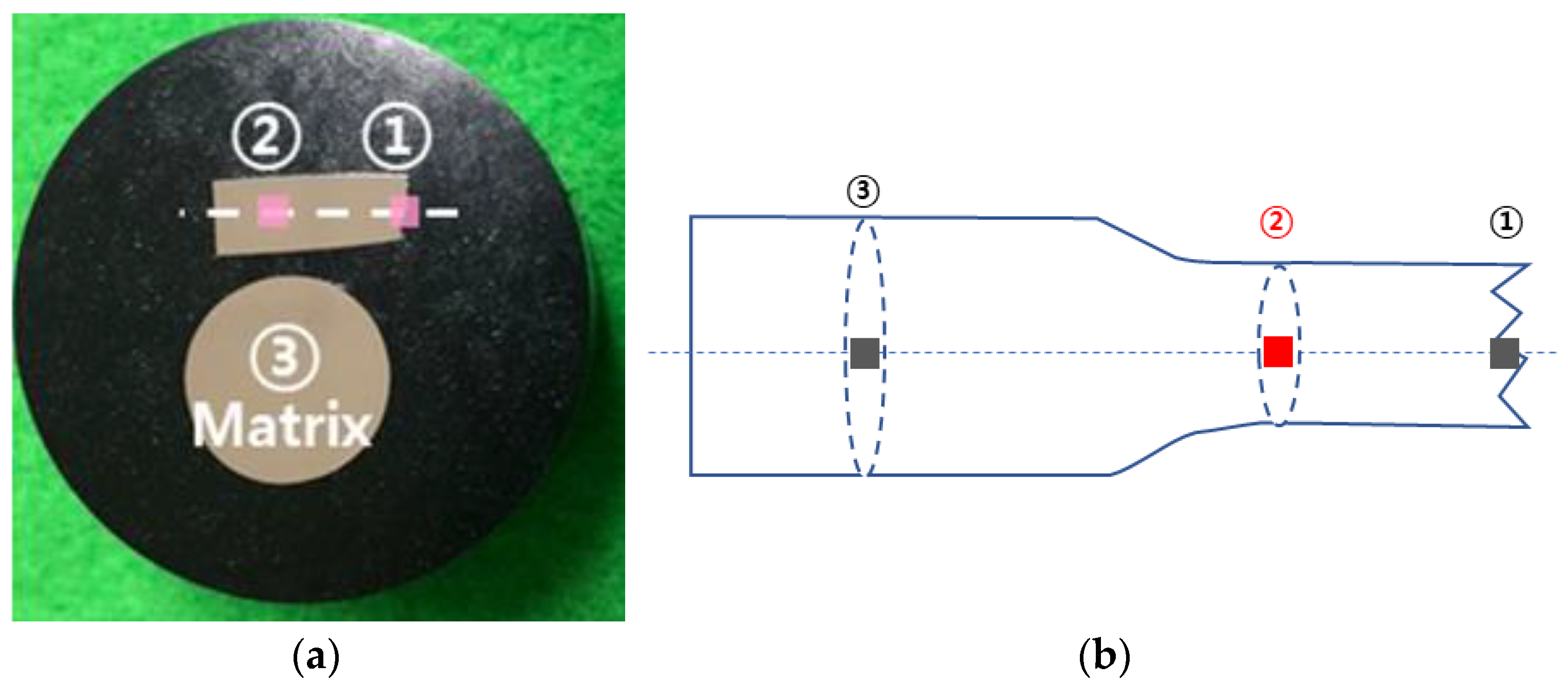
The material used for the test based on ASTM E139-11 [27] is DA-5161 SX, a nickel-based superalloy used in the manufacture of turbine blades. Sixteen environmental conditions (stress, temperature) were used to measure the time to breakage. The fractured specimens were cut at an appropriate position (position 2 in Figure 4b) to observe the effect of environmental conditions on the material as shown in Figure 4a,b. SEM (Hitachi Model S-3400N) images and microstructure images were taken. Processing the specimen before shooting involved sequential grinding using abrasive paper #200, #400, #600, #800, and #1000. As a final polishing step, 1 μm of colloidal silica was used for polishing for 1 h or more. Etching was performed with Marble’s reagent (10 g ${\mathrm{CuSO}}_4$ + 50 mL HCl + 50 mL distilled water). About 30 to 120 images per specimen, a total of 991 images, were taken at different locations in the same specimen tested under 16 environmental conditions. The accelerating voltage was 20 kV, the magnification was from ×2.00 k to ×5.00 k, the working distance was from 6.2 mm to 10.1 mm, and the image size was 1280 × 960. As shown in Figure 5, as the material is subjected to extreme environmental conditions, the size of the gamma-prime image increases in the image with the same magnification, and the shape becomes longer or merges with the adjacent gamma-prime image. As a change in texture was observed due to such degradation, characteristics such as volume fraction of gamma/gamma prime and aspect ratio according to rafting of gamma prime were utilized for traditional degradation analysis.

2.1.2. Data Preprocessing

As shown in Figure 6, a region of interest (ROI) is extracted from the acquired image data for each environmental condition so that only the tissue image can be seen (excluding the photography conditions at the bottom). The size of the image is reduced from 1280 × 960 to 1280 × 896. A training image for the segmentation model was constructed by performing annotation on 52 images for the region prediction model on the gamma prime corresponding to the region-of-interest image. A deep learning model was created through U-Net, where the input image is 224 × 224 × 3, and the output image has the form of 224 × 224 × 1. The total number of parameters is about 22 million, of which about 8 million are used for training. The regions of interest of the 991 creep test images used for this study are the input of the learned U-Net and the binarized image (gamma-prime phase: black; gamma phase: white) in which the region on the gamma prime is predicted as the output for deep learning. We can quickly characterize the gamma-prime phase using the model. There are 16 test environmental conditions as shown in

Table 3. Normalized creep test environmental information and time-to-rupture data.

Test No.	Temperature	Stress	Rupture Time
1	0.1000	0.5656	0.6832
2	0.5000	0.3027	0.3971
3	0.7000	0.1964	0.4802
4	0.9000	0.1605	0.2081
5	0.5000	0.2681	0.6596
6	0.7000	0.1698	0.8178
7	0.9000	0.1000	0.9000
8	0.1000	0.6704	0.2823
9	0.5000	0.3399	0.2398
10	0.7000	0.2258	0.2589
11	0.9000	0.1408	0.3231
12	0.1000	0.6166	0.4825
13	0.1000	0.9000	0.1168
14	0.5000	0.4913	0.1060
15	0.7000	0.3420	0.1000
16	0.9000	0.2278	0.1075

, and the temperature, stress, break time, and LMP for each condition were processed to have values between 0.1 and 0.9 through Min–Max normalization.

2.2. Methods

As shown in Figure 7, a new degradation index quantification method was proposed, (the model learning method), and the performance of various regression models for each geometric feature on the gamma prime were compared using the degradation index and LMP. We also tried to determine whether or not the model performance was improved if a significant explanatory variable was selected. The Bayesian regression model and the Gaussian process regression model were used to infer the parameters (regression coefficient and error term) constituting the regression equation through Metropolis–Hastings sampling using MCMC. This intuitively explains the uncertainty of the prediction as a probability.

In the dataset of 991 images, 80% were randomly divided into training data (792 images) and 20% test data (199 images) for each environmental condition. The training data were used to quantify the degradation index and train the predictive model, and the test data were used to verify the performance of the predictive model.

The area of the gamma prime is predicted through U-Net from the microstructure image of the material obtained after the destructive test to quantify the degradation index. This results in a bag of images (BoI). After that, the geometric feature index of the microstructure is extracted to construct a bag of features (BoF), and the BoI-based significance cluster is determined using the non-parametric clustering method. The degradation index is extracted from the significant cluster learned for the image to be evaluated for the degree of degradation, and the representative degradation index is determined for images taken at different locations under the same experimental environment condition.

After responding to the representative values of the quantified degradation index for each environmental condition, the degradation index prediction model is constructed by learning the regression model using the environmental condition information as the explanatory variable and the degradation index as the response variable. At this time, a significant explanatory variable and a polynomial regression order are selected that consider the alternating variables of the explanatory variables. Ordinary least squares (OLS), generalized linear model (GLM), Bayesian regression (BR), and Gaussian process regression (GPR) models were used for the regression model. BR and GPR are Bayesian models that infer the posterior distribution of parameters. In the LMP prediction model, the degradation index with one or several geometric features deduced from the microstructure image are input as explanatory variables by reducing the dimension, and the response variable is the theoretical value LMP calculated using Equation (1) for learning. Four types of regression models were trained including the degradation index prediction model.

As an inference method for the degradation index and LMP prediction model, the degradation index for geometric features is predicted when the exposure time to the temperature, stress, and environment to be evaluated is input to the degradation index prediction model. The predicted degradation index is then input into the LMP prediction model, and the values of the LMP are simultaneously predicted. In the case of predicting LMP by inputting a replica microstructure image, the degradation index is extracted, and LMP is predicted using it as an input to the learned LMP prediction model after predicting the gamma-prime phase region with U-NET.

2.2.1. Quantification Method of Degradation Index

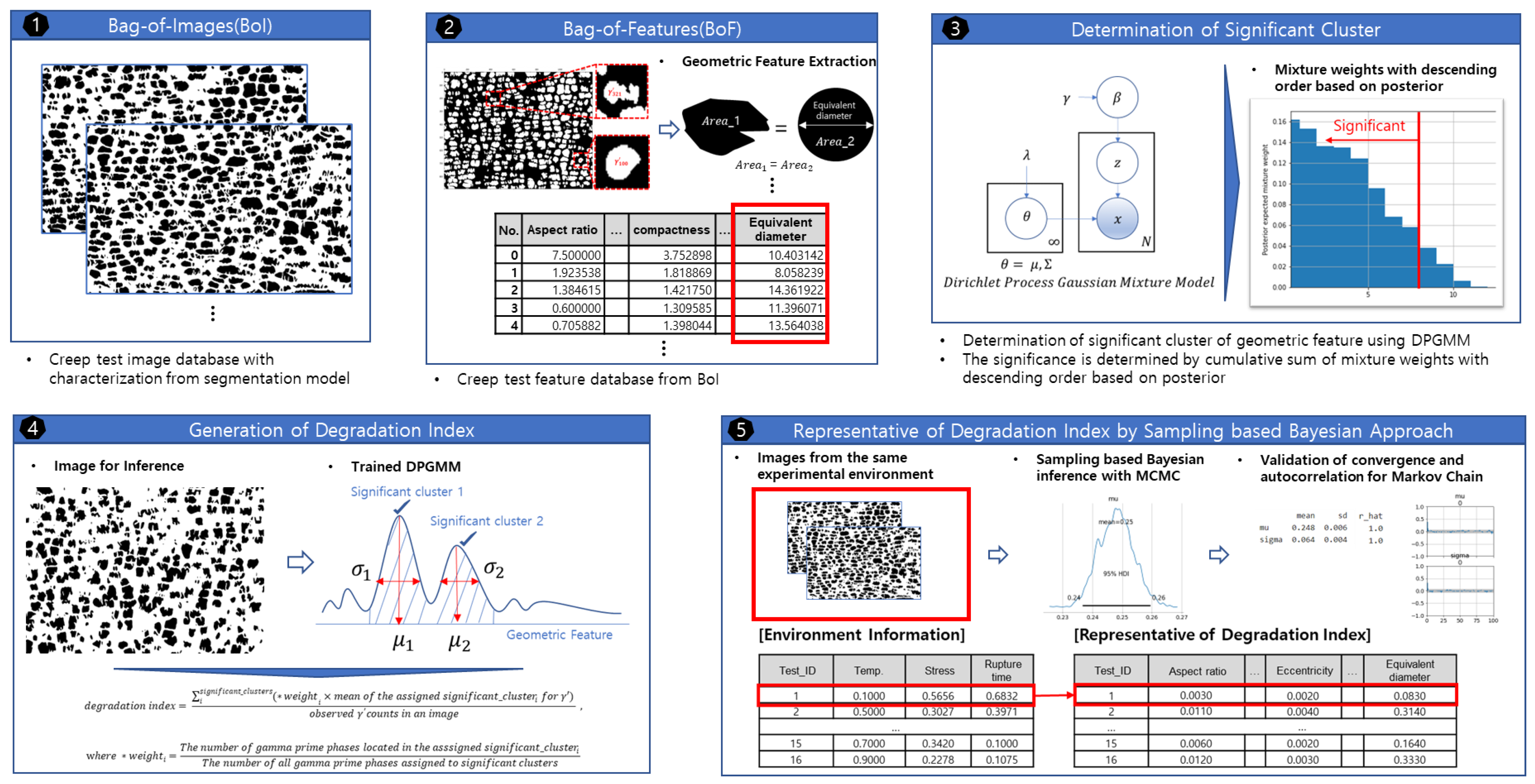
A method for quantifying the degradation index using a sampling-based Bayesian inference method proceeds in the order shown in Figure 8. After taking the SEM image, the microstructure gamma-prime phase is rapidly characterized through U-Net. Then, the region of the gamma/gamma-prime phase is binarized, accumulated, and stored in the destructive test database. This method was named BoI. If destructive tests such as creep tests are conducted for research in the future, environmental conditions used in the experiments and characterized image data are accumulated in BoI. This process saves the time required to classify the gamma/gamma-prime phase in the research process and can be used to infer the degradation index due to data accumulation close to the parameter.

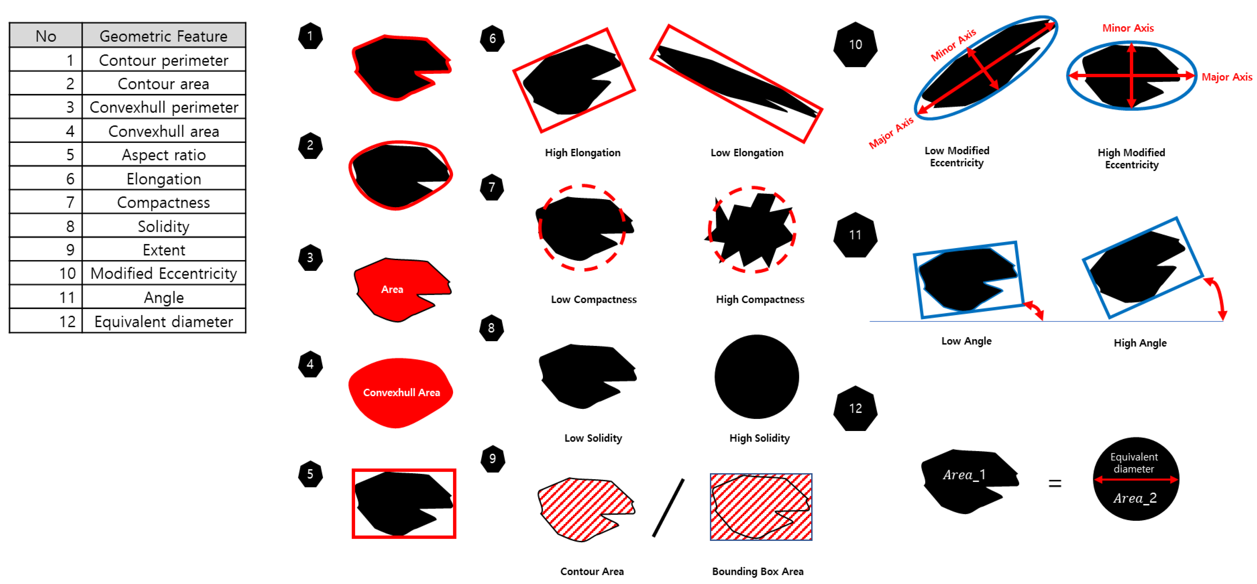
A BoF is formed when a BoI is configured. Here, a feature means a geometric feature of a gamma-prime image region existing in an image. Using the geometric features of the gamma prime, it is possible to explain the subsequent degradation index with the geometric features of the gamma prime. A total of 12 geometric features were used, as shown in Figure 9. A BoF is constructed by numerically quantifying geometric features on the gamma prime observed in all images in the BoI. Feature engineering is applied to quantify a specific value from the shape of the gamma prime in this process. Among the geometric features used in this study, the contour perimeter means the length of the perimeter of the gamma-prime image, and the contour area means the inner area of the gamma-prime image. The convex hull perimeter is the length of the perimeter that convexly surrounds the gamma-prime phase [28], and the convex hull area is the corresponding area. Aspect ratio refers to the aspect ratio of the bounding box surrounding the gamma-prime image as shown in Equation (2). The aspect ratio is traditionally used when judging the degree of rafting. In this study, the aspect ratio was defined as follows.

$$\mathrm{aspect} \mathrm{ratio}=\frac{\mathrm{width}}{\mathrm{height}},$$

(2)

Elongation is the value obtained by dividing the length of the short side by the length of the long side to the extent that the bounding box surrounding the gamma-prime image is stretched as shown in Equation (3) [29].

$$\mathrm{elongation}=\frac{{\mathrm{length}}_1}{{\mathrm{length}}_2}, ({\mathrm{length}}_1<{\mathrm{length}}_2),$$

(3)

In this study, compactness is redefined to have a dense contour perimeter for the contour area as in Equation (4), and the contour perimeter is deformed compared to a circle. In the case of a circle, it has a value of 1, and the compactness value increases for more complex shapes [29].

$$\mathrm{compactness}=\frac{{\mathrm{contour} \mathrm{perimeter}}^2}{4\mathsf{\pi }\times \mathrm{contour} \mathrm{area}},$$

(4)

Solidity is an index that can measure concavity as in Equation (5), and it has a value of 1 in the case of a circle or an ellipse [29].

$$\mathrm{solidity}=\frac{\mathrm{contour} \mathrm{area}}{\mathrm{convexhull} \mathrm{area}},$$

(5)

Modified eccentricity is defined as the ratio of the length of the major axis to the length of the minor axis of the ellipse surrounding the object as shown in Equation (6). This is different from eccentricity, and it is defined as modified eccentricity considering the point using the axis length of the ellipse [29].

$$\mathrm{modified} \mathrm{eccentricity}=\frac{\mathrm{minor} \mathrm{axis} \mathrm{length}}{\mathrm{major} \mathrm{axis} \mathrm{length}} ,$$

(6)

Angle indicates the inclined angle of the bounding box surrounding the object, and equivalent diameter means the diameter of a circle having the same area as the area of the object as in Equation (7).

$$\mathrm{equivalent} \mathrm{diameter}=\sqrt{\frac{4\times \mathrm{contour} \mathrm{area}}{\mathsf{\pi }}} ,$$

(7)

In this study, a BoF was constructed based on 792 pieces of learning data, and 156,862 quantified feature values for each of 12 geometric features were obtained. For each geometric feature, unsupervised learning was performed with DPGMM, and the mixture weights based on the posterior distribution were listed in descending order to determine the cluster. A cumulative sum of 0.9 was chosen as a significant cluster. DPGMM is a Bayesian-based non-parametric clustering model. It has the advantage of being able to determine the number of clusters based on observation data without prior definition of the number of clusters as in the above method. The DPGMM model is trained with the training data, and the gamma-prime image for the new image is assigned as a significant cluster from the DPGMM for each learned geometric feature. To determine the degradation index for each image, geometric features are calculated for each gamma-prime image region, and feature values can be obtained based on the number of gamma-prime images existing in the image. To avoid increasing the dimension of the feature explaining the degradation of the image by the number of gamma-prime phases, we propose a method in which one geometric feature value can be extracted from one image. Using the mean vector and covariance matrix of the clusters of DPGMM learned for each geometric feature, the cluster with the highest probability value in the probability of multivariate normal distribution is determined as the cluster of geometric feature values on gamma prime. The geometric feature corresponds to the determined significant cluster. The degradation index can be defined using the feature value as in Equation (8) below.

$$\mathrm{degradation} \mathrm{index}=\frac{{{\displaystyle \sum }}_{\mathrm{i}}^{\mathrm{significant}\_\mathrm{clusters}}({\ast \mathrm{weight}}_{\mathrm{i}}\times \mathrm{mean} \mathrm{of} \mathrm{the} \mathrm{assigned} \mathrm{significant}\_{\mathrm{cluster}}_{\mathrm{i}} \mathrm{for} {\mathsf{\gamma }}^{\prime }) }{\mathrm{observed} {\mathsf{\gamma }}^{\prime } \mathrm{counts} \mathrm{in} \mathrm{an} \mathrm{image}} ,$$

(8)

$$\mathrm{where} {\ast \mathrm{weight}}_{\mathrm{i}}=\frac{\mathrm{The} \mathrm{number} \mathrm{of} \mathrm{gamma} \mathrm{prime} \mathrm{phases} \mathrm{located} \mathrm{in} \mathrm{the} \mathrm{asssigned} \mathrm{significant}\_{\mathrm{cluster}}_{\mathrm{i}}}{\mathrm{The} \mathrm{number} \mathrm{of} \mathrm{all} \mathrm{gamma} \mathrm{prime} \mathrm{phases} \mathrm{assigned} \mathrm{to} \mathrm{significant} \mathrm{clusters}}.$$

Equation (8) selects only gamma-prime phases corresponding to significant clusters and removes feature values of non-sected gamma-prime phases. After determining significant clusters, gamma primes belonging to non-significant clusters are excluded from the indexing process, which has the effect of removing outliers that hinder the determination of values representing microstructure images. In addition, the segmentation prediction error can also provide a robust and significant gamma-prime phase despite image noise. To reinforce the influence of gamma-prime phase clusters that provide the key information in the image, a weighted average is obtained as a ratio of the number assigned to each cluster to the total number of significant gamma-prime phases in the image. Finally, we tried to capture information on the number of gamma-prime images observed at the same magnification in the degradation index by dividing it by the total number of gamma-prime images present in the image.

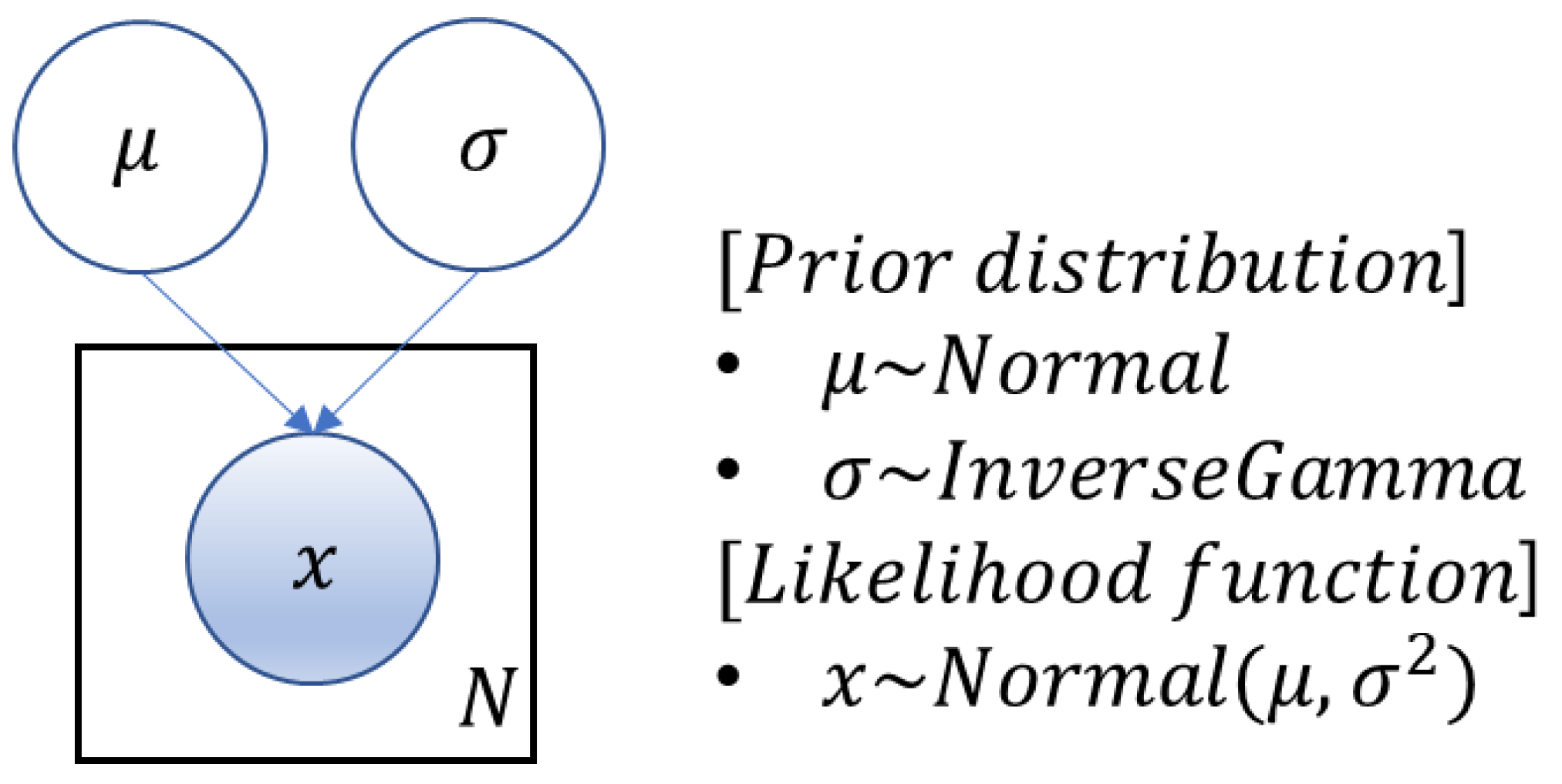
A value capable of representing the degradation indices of dozens of images taken under the same test conditions is selected as a degradation index for each microstructure image. A representative value of the degradation index was set using a sampling-based Bayesian inference method based on MCMC. As shown in Figure 10, MCMC and Metropolis–Hastings sampling were used to define the expected value of the posterior distribution for the average degradation index through sampling as the representative value of the degradation index. To secure the reliability of the posterior distribution of the representative value of the degradation index and the mean of the degradation index, it is necessary to test convergence and autocorrelation. In the convergence test, the value converged if the R hat value was within the range of 1 ± 0.05. If the effective sample size (ESS) was 500 or higher, it was judged to be a reliable Markov chain with low autocorrelation. Metropolis–Hastings sampling was iterated 10,000 times to meet the criteria of convergence and autocorrelation, and 4 Markov chains were run. To conduct this, thinning was performed every 5 samples. The distribution of the burn-in and thinning samples was evaluated by the posterior distribution, and the representative value of the degradation index was finally inferred as the expected value of the posterior distribution of μ among them. We inferred the representative value of the degradation index for each set of learning data and test data. The variability of the degradation index inferred from the learning data and test data for each identical environmental condition was quantified by Equation (9), and the results are shown in

Table 4. Degradation index representative value inference result volatility comparison table.

Degradation Index	Variation of Degradation Index between Train and Test Datasets
Contour perimeter	11.41%
Contour area	12.95%
Convex hull perimeter	11.74%
Convex hull area	12.34%
Aspect ratio	14.10%
Elongation	24.93%
Compactness	11.01%
Solidity	12.10%
Extent	12.96%
Modified eccentricity	20.16%
Angle	6.85%
Equivalent diameter	11.77%
Average	13.53%

.

$$\frac{{{\displaystyle \sum }}_{\mathrm{i}}^{\mathrm{N}}\frac{\left|{\mathrm{DI}}_{\mathrm{i}}^{\mathrm{train}}-{\mathrm{DI}}_{\mathrm{i}}^{\mathrm{test}}\right|}{{\mathrm{DI}}_{\mathrm{i}}^{\mathrm{train}}}}{\mathrm{N}}\times 100(\%),$$

(9)

Here, ${\mathrm{DI}}_{\mathrm{i}}^{\mathrm{train}}$ means the degradation index representing the image of the ith experimental environmental condition in the training data, ${\mathrm{DI}}_{\mathrm{i}}^{\mathrm{test}}$ means the degradation index representing the image of the ith experimental environmental condition in the learning data, and N is the number of environmental conditions, which is 16 in this case. The variability of the degradation index for each of the 12 geometric features inferred from the training and test image data was 13.53% on average, and the highest variability was observed for elongation. Five types of degradation indexes were listed as geometric features in order of smallest variability. Angle was the smallest at 6.85%, followed by compactness, contour perimeter, convex hull perimeter, and equivalent diameter.

2.2.2. Degradation Index Prediction Model

A degradation index prediction model can be learned from the representative degradation index values corresponding to each of the 16 experimental environmental conditions from the learning image data as a response variable, while the environmental conditions (temperature, stress, time) of the material were used as an explanatory variable. OLS, GLM, BR, and GPR were used as regression models. Performance changes were observed according to whether or not the process of selecting significant explanatory variables was used for each model. In the case of the BR and GPR models, prediction is possible with an explanation of uncertainty even for explanatory variables that are not observed in the training data. BR and GPR view the parameters of each model as random variables, predicting the posterior distribution of parameters from samples extracted using MCMC and Metropolis–Hastings sampling. This can be used to explain the model from the statistics of the posterior distribution.

The method of dimensionally reducing environmental conditions (temperature, stress, time) as explanatory variables into one principal component (PC) through PCA and the method of selecting two significant variables in order of importance through LASSO regression were compared. Reducing explanatory variables to one or two dimensions is performed to support intuitive interpretation when visualizing regression models.

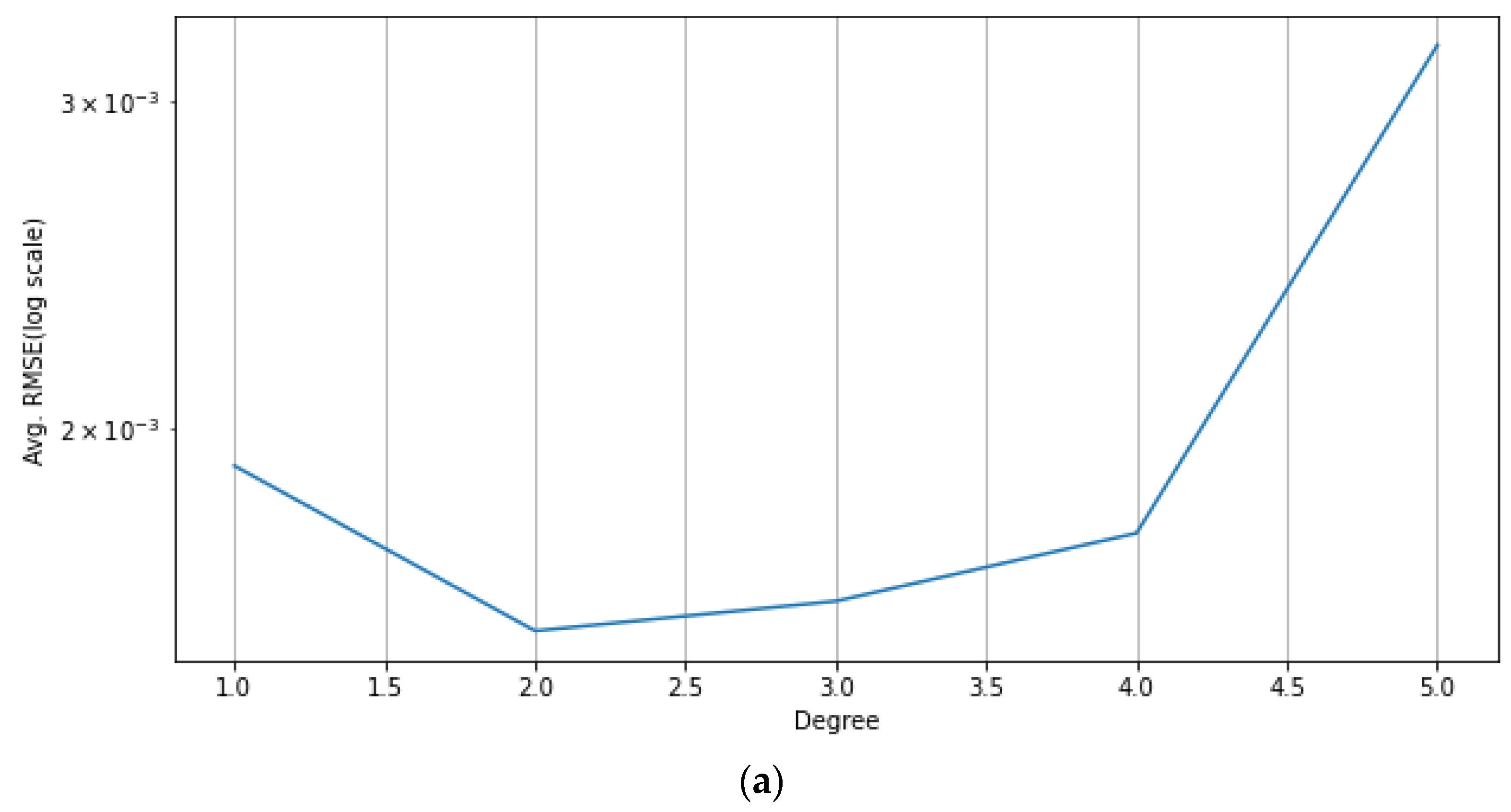
As in the example of Figure 11a, the principal component is the explanatory variable, while the degradation index based on the geometric features is used as the response variable for the learning data when dimensionality reduction is performed with one principal component. After 5-fold cross-validation of polynomial regression from order 1 to order 5, the order with the lowest RMSE value is determined as the appropriate order.

As shown in the example in Figure 11b, the three variables temperature, stress, and time are standardized in the process of selecting two significant explanatory variables. The degradation index based on the explanatory variable and geometric feature is used as the response variable. Cross-validation was performed by transforming the hyperparameter α representing the regularization strength of the LASSO regression (including the interaction variables from the 1st to the 4th order, 5-fold) to find the regression order and α combination with the largest negative mean squared error. This combination was selected as the final significant variables in the order of the largest absolute values of the regression coefficients.

Table 5. Explanatory variable selection result table of degradation index prediction model.

Degradation Index	Selected Input Variable
Contour perimeter	1. Temperature × Time, 2. Temperature
Contour area	1. Temperature × Time, 2. Stress
Convex hull perimeter	1. Temperature × Time, 2. Temperature
Convex hull area	1. Temperature × Time, 2. Temperature
Aspect ratio	$1. {\mathrm{Temperature}}^2\times \mathrm{Time}$ $2. {\mathrm{Temperature}}^2\times \mathrm{Stress}\times \mathrm{Time}$
Elongation	1. Temperature × Time, 2. Time
Compactness	$1. {\mathrm{Temperature}}^2\times \mathrm{Time}$ 2. Temperature × Time
Solidity	$1. {\mathrm{Temperature}}^2\times \mathrm{Time}$ 2. Temperature × Time
Extent	$1. {\mathrm{Temperature}}^2\times \mathrm{Time}$ 2. Temperature × Time
Modified eccentricity	1. Temperature × Time, 2. Time
Angle	$1. {\mathrm{Temperature}}^2\times \mathrm{Time}$ 2. Temperature × Time
Equivalent diameter	1. Temperature × Time, 2. Stress

shows the finally selected explanatory variables for each degradation index having geometric characteristics.

For the training data, the explanatory variables were set as values consisting of one main component of temperature, stress, and time or significant variables selected from Table 5. Four regression models (OLS, GLM, BR, GPR) were constructed.

OLS is a method of finding the regression coefficient that minimizes the residual between the predicted value and the actual value of the regression model using the least squares method.

$$\begin{gathered} \underset{\mathsf{\Theta }}{\mathrm{argmin}}\mathrm{E}\left(\mathsf{\Theta }\right)=\underset{\mathsf{\Theta }}{\mathrm{argmin}}{\displaystyle {\sum }_{\mathrm{i}=1}^{\mathrm{n}}}{\left(\widehat{{\mathrm{y}}_{\mathrm{l}}}-{\mathrm{y}}_{\mathrm{i}}\right)}^2, \\ \mathrm{where} \mathsf{\Theta }=\left({\mathsf{\theta }}_0,{ \mathsf{\theta }}_1, \dots ,{ \mathsf{\theta }}_{\mathrm{k}}\right),\widehat{{\mathrm{y}}_{\mathrm{l}}}={\mathsf{\theta }}_0+{\mathsf{\theta }}_1{\mathrm{x}}_{\mathrm{i}}+\dots +{\mathsf{\theta }}_{\mathrm{k}}{\mathrm{x}}_{\mathrm{i}}^{\mathrm{k}} \end{gathered}$$

(10)

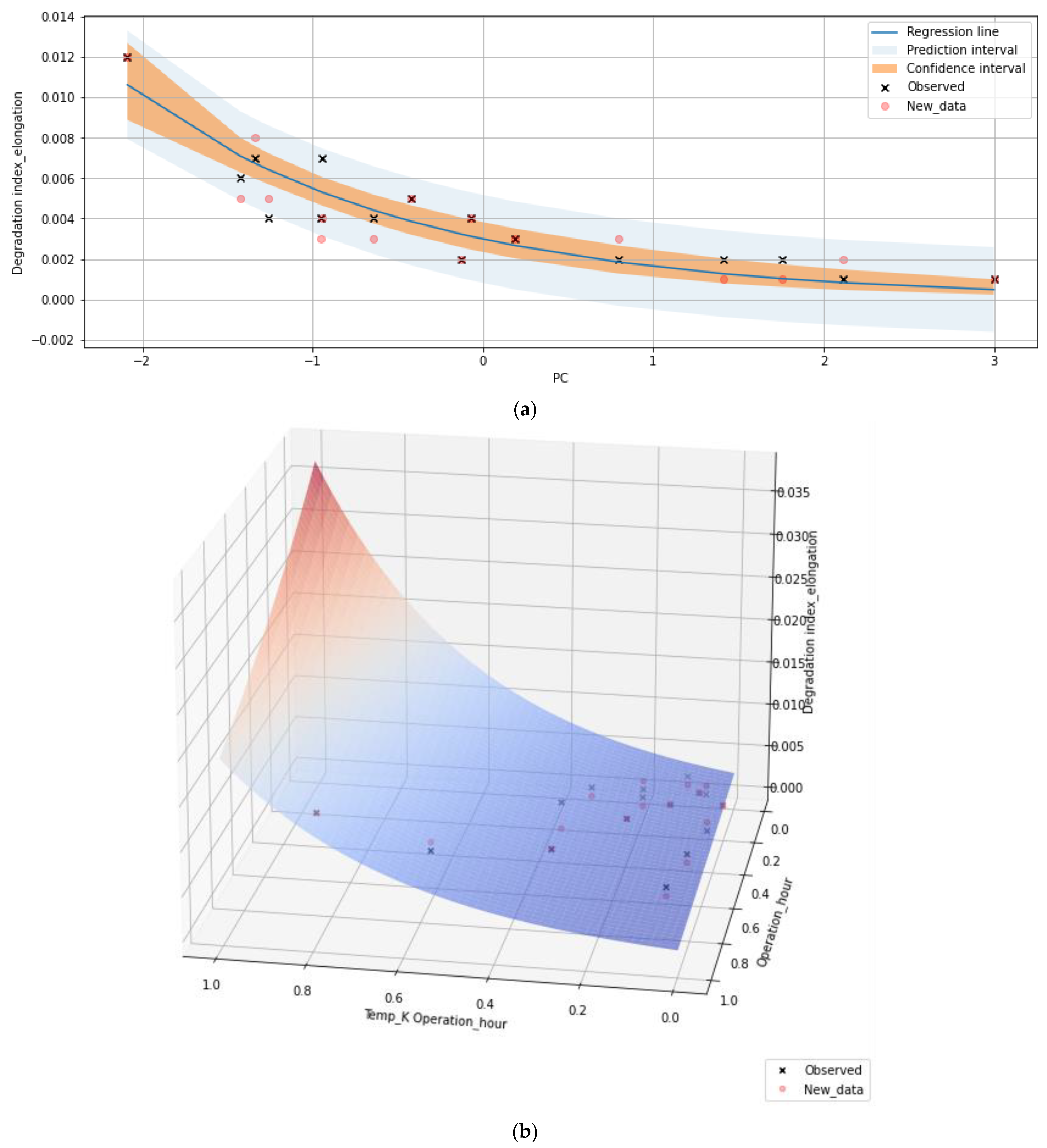
Here, $\mathrm{E}\left(\mathsf{\Theta }\right)$ is the error term, $\widehat{{\mathrm{y}}_{\mathrm{l}}}$ is the predicted value of the ith data, ${\mathrm{y}}_{\mathrm{i}}$ is the actual value of the ith data, n is the number of datapoints, ${\mathrm{x}}_{\mathrm{i}}$ is the input value corresponding to the explanatory variable of the ith data, and k is the order of polynomial regression. The regression coefficient ${\mathsf{\theta }}_{\mathrm{k}}$ that $\mathrm{E}\left(\mathsf{\Theta }\right)$ minimizes can be found when the partial derivative of $\mathrm{E}\left(\mathsf{\Theta }\right)$ with the regression coefficient ${\mathsf{\theta }}_{\mathrm{k}}$ becomes 0. In this study, there are two cases of a second-order OLS polynomial regression model using one principal component as an explanatory variable as in Equation (11) and a regression model in which two significant explanatory variables are selected for the degradation index for each geometric feature as in Equation (12). A model was constructed, and the prediction result model and average confidence interval and prediction interval were visualized as shown in Figure 12a,b.

$$\begin{gathered} \mathrm{y}={\mathsf{\theta }}_0+{\mathsf{\theta }}_1{\mathrm{PC}}_1+{\mathsf{\theta }}_2{\mathrm{PC}}_1^2+\mathsf{\epsilon }, \\ \mathrm{where} \mathsf{\epsilon }~\mathrm{N}\left(0,{ \mathsf{\sigma }}^2\right) \end{gathered}$$

(11)

$$\begin{gathered} \mathrm{y}={ \mathsf{\theta }}_0+{\mathsf{\theta }}_1·\mathrm{selected}\_{\mathrm{variable}}_1+{\mathsf{\theta }}_2·\mathrm{selected}\_{\mathrm{variable}}_2+\mathsf{\epsilon }, \\ \mathrm{where} \mathsf{\epsilon }~\mathrm{N}\left(0,{ \mathsf{\sigma }}^2\right) \end{gathered}$$

(12)

GLM is a generalized linear model shown in Equation (13). GLM can be used even when the data type of the response variable of the linear model is continuous or categorical.

$$\begin{gathered} \mathrm{g}\left(\mathsf{\mu }\right)=\mathrm{g}\left(\mathrm{E}\left({\mathrm{Y}|\mathrm{x}}_1, \dots ,{ \mathrm{x}}_{\mathrm{n}}\right)\right)=\mathrm{g}\left({\mathsf{\theta }}_0+{\mathsf{\theta }}_1{\mathrm{x}}_1+\dots +{\mathsf{\theta }}_{\mathrm{n}}{\mathrm{x}}_{\mathrm{n}}\right), \\ \mathrm{where} \mathrm{g}\left( · \right)=\mathrm{link} \mathrm{function} \end{gathered}$$

(13)

The limitation occurring when the range of the linear prediction value and the range of μ are different can be solved through a link function. In this study, models were constructed for two cases: a GLM using one principal component as an explanatory variable as shown in Equation (14) and a GLM using two significant explanatory variables for the degradation index for each geometric feature as shown in Equation (15). The prediction result model and average confidence interval and prediction interval are visualized in Figure 13a,b.

$$\begin{gathered} \ln \left(\mathsf{\mu }\right)=\ln \left(\mathrm{E}\left({\mathrm{Y}|\mathrm{PC}}_1\right)\right)=\ln \left({\mathsf{\theta }}_0+{\mathsf{\theta }}_1{\mathrm{PC}}_1\right), \\ \mathrm{where} \mathrm{link} \mathrm{function}=\ln \left(·\right) \end{gathered}$$

(14)

$$\begin{gathered} \ln \left(\mathsf{\mu }\right)=\ln (\mathrm{E}\left({\mathrm{Y}|\mathrm{Selected} \mathrm{variable}}_1,{ \mathrm{Selected} \mathrm{variable}}_2)=\ln ({\mathsf{\theta }}_0+{\mathsf{\theta }}_1{\mathrm{Selected} \mathrm{variable}}_1+{\mathsf{\theta }}_2{\mathrm{Selected} \mathrm{variable}}_2\right), \\ \mathrm{where} \mathrm{link} \mathrm{function}=\ln \left(·\right) \end{gathered}$$

(15)

BR and GPR are based on Bayesian statistics. The most fundamental theory in Bayesian statistics is Bayes’ Theorem, which is the following equation.

$$\begin{gathered} \mathrm{P}\left(\mathrm{w}|\mathrm{D}\right)=\frac{\mathrm{P}\left(\mathrm{D}|\mathrm{w}\right)\mathrm{P}\left(\mathrm{w}\right)}{\mathrm{P}\left(\mathrm{D}\right)}, \\ \mathrm{where} \mathrm{P}\left(\mathrm{D}\right)={\displaystyle \int }\mathrm{P}\left(\mathrm{D}|\mathrm{w}\right)\mathrm{P}\left(\mathrm{w}\right)\mathrm{dw} \end{gathered}$$

(16)

Here, P(D|w) is a likelihood function and expresses how likely the observed dataset is to appear for each parameter vector w. P(w) is a prior probability distribution, which can be viewed as the degree of belief using previous knowledge, and it is an assumption about w before observing data. P(w|D) is the posterior probability distribution, which updates the prior probability distribution in proportion to the product of the prior probability distribution and the likelihood. From the frequentist probability point of view, w is a fixed parameter, but from the Bayesian probability point of view, only the actually observed dataset D exists, and the uncertainty of the parameter is expressed through the probability distribution w. When the number of observed data increases infinitely, the result of probability from the frequentist viewpoint and the probability from the Bayesian viewpoint converge to the same value [30].

In Bayesian inference, it is necessary to calculate the joint posterior distribution for a set of parameters, but the calculation of the integral is actually difficult, and the difficulty increases as the dimensionality increases. Thus, it becomes difficult to solve the problem through an analytical equation. The MCMC method and the variational inference method are mainly used to solve this problem as they can approximate the posterior distribution of parameters. Using the MCMC method, the posterior distribution and difficult-to-calculate integrals can be used as a way to practically enable inference with samples from the posterior distribution as simulation results. Metropolis–Hastings sampling and Gibbs sampling are representative sampling-based Bayesian inference methods, but Bayesian inference was performed based on the Metropolis–Hastings sampling algorithm shown in Algorithm 1 in this study. The Metropolis–Hastings sampling method is as follows: (1) A proposal (candidate) sample ${\mathrm{x}}^{\mathrm{candidate}}$ is sampled from the proposal distribution $\mathrm{q}({\mathrm{x}}^{\left(\mathrm{i}\right)}|{\mathrm{x}}^{\left(\mathrm{i}-1\right)})$. (2) The acceptance probability is calculated based on the offer distribution and the joint distribution $\mathsf{\pi }\left(·\right)$ from the acceptance function $\mathsf{\alpha }({\mathrm{x}}^{\mathrm{candidate}}|{\mathrm{x}}^{\left(\mathrm{i}-1\right)})$. (3) Proposal (candidate) sample ${\mathrm{x}}^{\mathrm{candidate}}$ is adopted with an acceptance probability α and is not adopted with a probability of 1 − α. Samples that are not adopted are replaced with previous samples ${\mathrm{x}}^{\left(\mathrm{i}-1\right)}$ [31,32].

Algorithm 1. Metropolis–Hastings Algorithm [31,32]

Initialize ${\mathrm{x}}^{\left(0\right)}~\mathrm{q}\left(\mathrm{x}\right)$

for iteration $\mathrm{i}=1,2,,\dots$ do

Propose: ${\mathrm{x}}^{\mathrm{candidate}}~\mathrm{q}({\mathrm{x}}^{\left(\mathrm{i}\right)}|{\mathrm{x}}^{\left(\mathrm{i}-1\right)})$

Acceptance Probability:

$\mathsf{\alpha }\left({\mathrm{x}}^{\mathrm{candidate}}{|\mathrm{x}}^{\left(\mathrm{i}-1\right)}\right)=\min \left\{1,\frac{ \mathrm{q}({\mathrm{x}}^{\left(\mathrm{i}-1\right)}|{\mathrm{x}}^{\mathrm{candidate}})\mathsf{\pi }\left({\mathrm{x}}^{\mathrm{candidate}}\right)}{\mathrm{q}({\mathrm{x}}^{\mathrm{candidate}}|{\mathrm{x}}^{\left(\mathrm{i}-1\right)})\mathsf{\pi }\left({\mathrm{x}}^{\left(\mathrm{i}-1\right)}\right)}\right\}$

$\mathrm{u}~\mathrm{Uniform}\left(\mathrm{u};0, 1\right)$

if $\mathrm{u}<\mathsf{\alpha }$ then

Accept the proposal: ${\mathrm{x}}^{\left(\mathrm{i}\right)}\leftarrow {\mathrm{x}}^{\mathrm{candidate}}$

else

Reject the proposal: ${\mathrm{x}}^{\left(\mathrm{i}\right)}\leftarrow {\mathrm{x}}^{\left(\mathrm{i}-1\right)}$

end if

end for

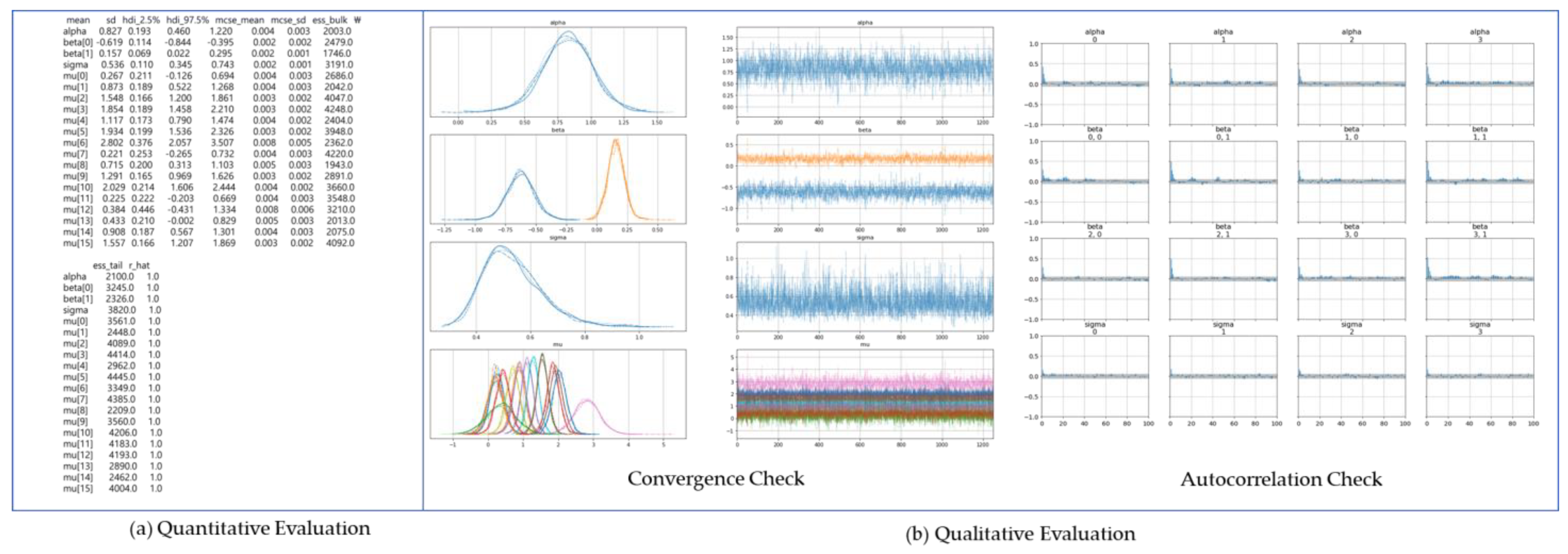
As shown in Figure 14, qualitative evaluation was performed using a graph visualizing the sampling iteration to evaluate whether the Markov chain for the posterior distribution of the parameter to be inferred as a result obtained after MCMC performed iteration was sufficiently converged. Convergence was quantitatively determined when the $\hat{\mathrm{R}}$ value was less than 1.05 or greater than 0.95. The autocorrelation was qualitatively evaluated according to the lag through the autocorrelation plot, which determined whether the autocorrelation had no pattern in a specific direction and was sufficiently small. The reliability of the Markov chain was evaluated based on whether the ESS was 500 or more. In this study, BR and GPR operated 20,000 iterations of Metropolis–Hastings sampling and 4 Markov chains to learn the degradation prediction model. To satisfy the $\hat{\mathrm{R}}$ value, 10,000 samples were burned in, and thinning was performed every 8 samples to satisfy the autocorrelation criterion. The distribution of the samples after burn-in and thinning was evaluated as the final posterior distribution. After the posterior distribution for the parameters is generated, the value of the response variable for the new explanatory variable can be predicted using the posterior distribution as shown in Equation (17) to predict new data ${\mathrm{x}}^{*}$.

$$\mathrm{P}\left({\mathrm{y}}^{*}{|\mathrm{x}}^{*}, \mathrm{y}\right)={\displaystyle \int }\mathrm{P}\left({\mathrm{y}}^{*}{|\mathrm{x}}^{*}, \mathrm{w}\right)\mathrm{P}\left(\mathrm{w}|\mathrm{y}\right)\mathrm{dw},$$

(17)

Here, y is the observed response variable, and w is the parameter we want to infer. x* is the new explanatory variable input we want to predict, y* is the predicted response variable for the explanatory variable x*, and P(w|y) is the posterior distribution for the parameters. Since it is difficult to calculate the integral with the posterior prediction distribution, an analytic solution can be avoided through a sampling-based approximation. In an intuitive interpretation, a sample of w is generated from the posterior distribution, and prediction is made through interval estimation by sampling new explanatory variables ${\mathrm{x}}^{*}$ and ${\mathrm{y}}^{*}$ considering the sampled w and precision β.

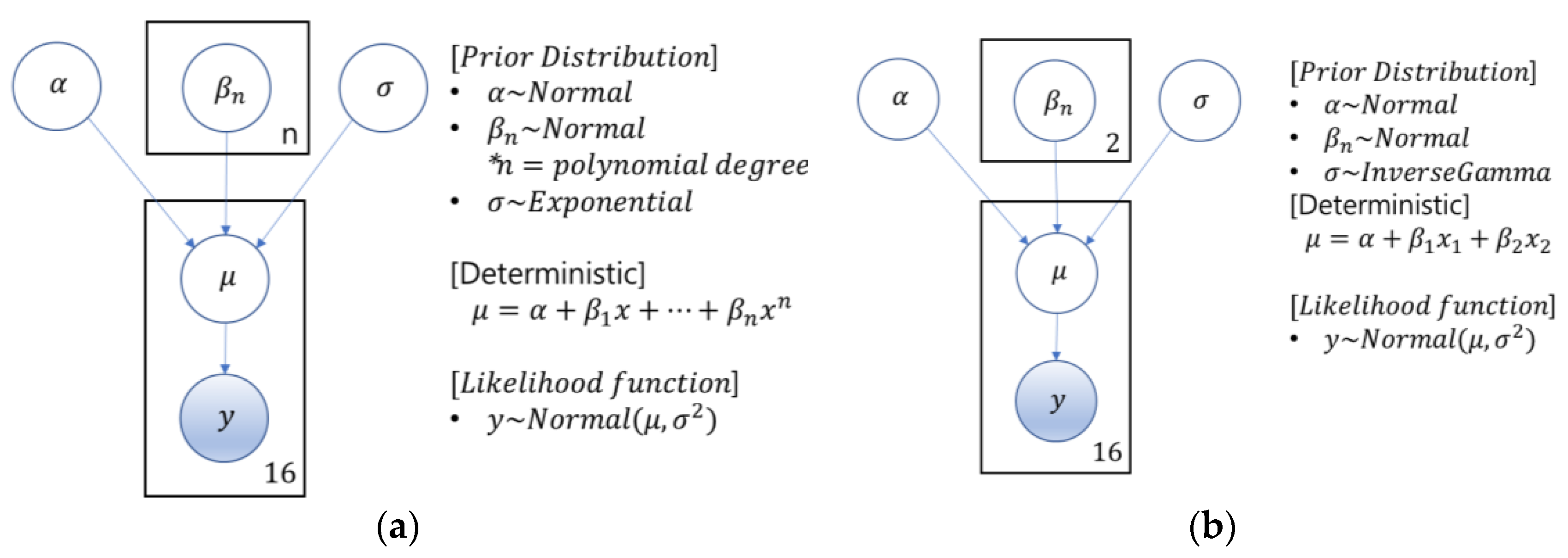
The BR model is configured as shown in Figure 15a,b, and the posterior distribution was inferred through MCMC and Metropolis–Hastings sampling considering the regression coefficient and error term as random variables. Figure 15a is a BR using one principal component as an explanatory variable, and Figure 15b is a Bayesian plate diagram of a BR in which the degradation index is predicted by selecting two significant explanatory variables to explain the degradation index for each geometric feature. As shown in Figure 16a,b, the BR prediction model and average credit interval and prediction interval were visualized.

In GPR, the output y of the function f as the input x is composed of “signal” (f) and “noise” (ε) as shown in Equation (18), and the signal part becomes a random variable following a specific distribution.

$$\begin{gathered} \mathrm{y}=\mathrm{f}\left(\mathrm{x}\right)+\mathsf{\epsilon }, \\ \mathrm{where} \mathsf{\epsilon }~\mathrm{N}\left(0,{ \mathsf{\sigma }}_{\mathsf{\epsilon }}^2\right) \end{gathered}$$

(18)

This distribution represents the uncertainty of f, and the uncertainty can be lowered by observing the output of the function for different input values. In GPR, f(x) follows the Gaussian process as shown in Equation (19).

$$\mathrm{f}\left(\mathrm{x}\right)~ \mathrm{GP}\left(\mathrm{m}\left(\mathrm{x}\right), \mathrm{k}\left(\mathrm{x}, {\mathrm{x}}^{\prime }\right)\right),$$

(19)

The Gaussian process (GP) is a distribution over a function and consists of a mean and a covariance function. The mean function and covariance function are defined as Equations (20) and (21):

$$\mathrm{m}\left(\mathrm{x}\right)=\mathrm{E}\left[\mathrm{f}\left(\mathrm{x}\right)\right],$$

(20)

$$\mathrm{k}\left(\mathrm{x}, {\mathrm{x}}^{\prime }\right)=\mathrm{E}[\left(\mathrm{f}\left(\mathrm{x}\right)-\mathrm{m}\left(\mathrm{x}\right)\right)(\mathrm{f}\left( {\mathrm{x}}^{\prime })-\mathrm{m}\left( {\mathrm{x}}^{\prime }\right))\right],$$

(21)

Here, x and x′ mean different input values. k is called the kernel of the Gaussian process, and an appropriate kernel is selected based on assumptions such as smoothness and similar patterns expected from the data. The most widely known kernel is the Radial Basis Function (RBF) kernel, which is defined in Equation (22):

$$\mathrm{k}\left(\mathrm{x}, {\mathrm{x}}^{\prime }\right)={\mathsf{\sigma }}_{\mathrm{f}}^2\exp \left(-\frac{{||\mathrm{x}-{\mathrm{x}}^{\prime }||}^2}{2{\mathsf{\lambda }}^2}\right),$$

(22)

In this kernel, $\mathsf{\lambda }$ is the length scale, and ${\mathsf{\sigma }}_{\mathrm{f}}^2$ is the signal variance, which lowers or increases the prior correlation between data points and consequently depends on the variability of the resulting function. ${\mathrm{X}}_{*}$ is a matrix where each row is a new input, ${\mathrm{x}}_{\mathrm{i}}\left(\mathrm{i}=1,\dots ,\mathrm{n}\right)$. To sample the function, we computed the covariance between the ${\mathrm{X}}_{*}$ phases to create an $\mathrm{n}\times \mathrm{n}$ matrix:

$$\mathrm{K}\left({\mathrm{X}}_{*},{ \mathrm{X}}_{*}\right)=\left[\begin{array}{ccc}\mathrm{k}\left({\mathrm{x}}_1^{*},{\mathrm{x}}_1^{*}\right)& \cdots & \mathrm{k}\left({\mathrm{x}}_1^{*},{\mathrm{x}}_{\mathrm{n}}^{*}\right)\\ ⋮& \ddots & ⋮\\ \mathrm{k}\left({\mathrm{x}}_{\mathrm{n}}^{*},{\mathrm{x}}_1^{*}\right)& \cdots & \mathrm{k}\left({\mathrm{x}}_{\mathrm{n}}^{*},{\mathrm{x}}_{\mathrm{n}}^{*}\right)\end{array}\right]$$

(23)

We can simplify the matrix computation by choosing the prior average function $\mathrm{m}\left(\mathrm{x}\right)=0$. By sampling from a multivariate normal distribution, we can sample f as ${\mathrm{X}}_{*}$ inputs from the $\mathrm{GP}$:

$$\begin{gathered} {\mathrm{f}}_{*}~\mathrm{N}\left(0, \mathrm{K}\left({\mathrm{X}}_{*},{\mathrm{X}}_{*}\right)\right), \\ {\mathrm{where} \mathrm{f}}_{*}={\left[\mathrm{f}\left({\mathrm{x}}_1^{*}\right),\dots ,\mathrm{f}\left({\mathrm{x}}_{\mathrm{n}}^{*}\right)\right]}^{\mathrm{T}} \end{gathered}$$

${\mathrm{f}}_{*}$ is a sample of one of the function values. A noise term, ε, must be added to sample ${\mathrm{y}}_{*}$, which is the prediction target. Observed data are ${\mathrm{D}}_{\mathrm{t}}=\left\{{\mathrm{X}}_{\mathrm{t}},{ \mathrm{y}}_{\mathrm{t}}\right\}$, and ${\mathrm{f}}_{*}$ is sampled from the posterior distribution $\mathrm{P}\left({\mathrm{f}|\mathrm{D}}_{\mathrm{t}}\right)$ to predict new input ${\mathrm{X}}_{*}$. By definition, the already observed ${\mathrm{y}}_{\mathrm{t}}$ and function values ${\mathrm{f}}_{*}$ follow the joint multivariate normal distribution:

$$\left[\begin{array}{c}{\mathrm{y}}_{\mathrm{t}}\\ {\mathrm{f}}_{*}\end{array}\right]~\mathrm{N}\left(0, \left[\begin{array}{cc}\mathrm{K}\left({\mathrm{X}}_{\mathrm{t}},{ \mathrm{X}}_{\mathrm{t}}\right)+{\mathsf{\sigma }}_{\mathsf{\epsilon }}^2\mathrm{I}& \mathrm{K}\left({\mathrm{X}}_{\mathrm{t}},{\mathrm{X}}_{*}\right) \\ \mathrm{K}\left({\mathrm{X}}_{*},{\mathrm{X}}_{\mathrm{t}}\right)& \mathrm{K}\left({\mathrm{X}}_{*},{\mathrm{X}}_{*}\right)\end{array}\right]\right),$$

where $\mathrm{K}\left({\mathrm{X}}_{\mathrm{t}},{ \mathrm{X}}_{\mathrm{t}}\right)$ is a covariance matrix between observed values, $\mathrm{K}\left({\mathrm{X}}_{*},{ \mathrm{X}}_{\mathrm{t}}\right)$ is a covariance matrix for new values, and $\mathrm{K}\left({\mathrm{X}}_{\mathrm{t}},{ \mathrm{X}}_{*}\right)$ is a covariance matrix between new values and previously observed values [33,34].

$$\mathrm{P}\left({\mathrm{f}}_{*}{|\mathrm{X}}_{\mathrm{t}},{ \mathrm{y}}_{\mathrm{t}},{ \mathrm{X}}_{*}\right)~\mathrm{N}(\mathrm{K}\left({\mathrm{X}}_{*},{\mathrm{X}}_{\mathrm{t}}\right){\left[\mathrm{K}\left({\mathrm{X}}_{\mathrm{t}},{\mathrm{X}}_{\mathrm{t}}\right)+{\mathsf{\sigma }}_{\mathsf{\epsilon }}^2\mathrm{I}\right]}^{-1}{\mathrm{y}}_{\mathrm{t}},\mathrm{K}\left({\mathrm{X}}_{*},{\mathrm{X}}_{*}\right)-\mathrm{K}\left({\mathrm{X}}_{*},{\mathrm{X}}_{\mathrm{t}}\right){\left[\mathrm{K}\left({\mathrm{X}}_{\mathrm{t}},{ \mathrm{X}}_{\mathrm{t}}\right)+{\mathsf{\sigma }}_{\mathsf{\epsilon }}^2\mathrm{I}\right]}^{-1}\mathrm{K}\left({\mathrm{X}}_{\mathrm{t}},{\mathrm{X}}_{*}\right))$$

In this study, the posterior distribution was approximated through MCMC and Metropolis–Hastings sampling, with ${\mathsf{\sigma }}_{\mathrm{f}}, \mathsf{\lambda },{ \mathsf{\sigma }}_{\mathsf{\epsilon }}$ (the hyperparameters in the RBF kernel of GPR) as random variables.

Figure 17a is a GPR using one principal component as an explanatory variable, and Figure 17b is a Bayesian plate diagram of GPR in which the degradation index is predicted by selecting two significant explanatory variables to explain the degradation index for each geometric feature. The GPR prediction model and average credit interval and prediction interval were visualized as shown in Figure 18a,b.

2.2.3. LMP Prediction Model

The LMP prediction model learning method is similar to the degradation prediction model learning method. The goal is to learn a regression model with degradation indices for each of 12 geometric features obtained from microstructure images as explanatory variables such that LMP that can be used to predict creep life as a response variable. OLS regression, GLM, and MCMC sampling-based BR and GPR were used as regression models to learn the following two cases: (1) a method of dimensionally reducing the degradation index having 12 geometric features extracted from microstructure images into one principal component and connecting the response variable to LMP and (2) a method of connecting each degradation index for each geometric feature as an explanatory variable and LMP as a response variable. Method (1) is intended to be used for intuitive evaluation by quantifying the creep life (even by non-experts) by quickly predicting LMP using the model with replication of high-temperature parts as input. Method (2) connects the learned LMP prediction model for each degradation index to the end of the degradation prediction model. When the environmental information of the material is input during the degradation simulation, the degradation index for each of 12 geometric features is output, and this is used as an input to the LMP prediction model so that the degradation index and LMP can be predicted at the same time.

Similar to the degradation prediction model learning method in Method (1), the dimensionality reduction of 12 degradation indices into one principal component (the RMSE value) is a result of 5-fold cross-validation of polynomial regression from order 1 to 5 with LMP as the response variable. This lowest order was determined as an appropriate order, and the third degree was deemed appropriate as a result of this study. Afterwards, 3rd-order polynomial OLS regression, GLM, and MCMC sampling-based BR and GPR were trained. BR and GPR predicted new explanatory variable values by generating samples from the posterior prediction distribution. Additionally, the top-5 significant variables were selected through LASSO regression in order of importance to explain the response variable (LMP) among geometric features. Dimensionality reduction and regression model learning were performed with one main component. This was tested to see if there was any change in performance compared to the LMP prediction model in which 12 degradation indices were dimensionally reduced as one principal component. Figure 19 visualizes the learning result of the Bayesian regression model based on sampling inference using explanatory variables after extracting 12 degradation indices from images.

3. Results

3.1. Evaluation Metric

3.1.1. Root-Mean-Squared Error (RMSE)

RMSE is a value obtained by taking the square root of the average of the squared differences between predicted values and actual values for all data. It is widely used as a performance indicator of regression models, and the units are the same as the units of the data, so you can intuitively determine the error of the model. A smaller model RMSE indicates a smaller difference between the predicted value and the actual value of the model. RMSE can be obtained as Equation (24):

$$\mathrm{RMSE}=\sqrt{{\displaystyle {\sum }_{\mathrm{i}=1}^{\mathrm{n}}}\frac{{\left(\widehat{{\mathrm{y}}_{\mathrm{l}}}-{\mathrm{y}}_{\mathrm{i}}\right)}^2}{\mathrm{n}}},$$

(24)

where $\widehat{{\mathrm{y}}_{\mathrm{l}}}$ is the predicted value of the i-th data, ${\mathrm{y}}_{\mathrm{i}}$ means the actual value of the ith data, and n indicates the number of datapoints.

3.1.2. R-Squared (R²)

${\mathrm{R}}^2$ is the coefficient of determination and can be interpreted as the degree of variance of the response variable that can be explained by the explanatory variable, and the goodness of fit of the regression model can be evaluated using Equation (25):

$${\mathrm{R}}^2=1-\frac{\mathrm{SSR}}{\mathrm{SST}}=1-\frac{{{\displaystyle \sum }}_{\mathrm{i}=1}^{\mathrm{n}}{\left({\mathrm{y}}_{\mathrm{i}}-\widehat{{\mathrm{y}}_{\mathrm{l}}}\right)}^2 }{{{\displaystyle \sum }}_{\mathrm{i}=1}^{\mathrm{n}}{\left({\mathrm{y}}_{\mathrm{i}}-\overline{\mathrm{y}}\right)}^2 },$$

(25)

where $\widehat{{\mathrm{y}}_{\mathrm{l}}}$ means the predicted value of the ith data, ${\mathrm{y}}_{\mathrm{i}}$ means the actual value of the ith data, $\frac{1}{\mathrm{n}}{\displaystyle \sum }_{\mathrm{i}=1}^{\mathrm{n}}{\mathrm{y}}_{\mathrm{i}}$, and $\mathrm{n}$ indicates the number of datapoints.

3.2. Degradation Index Prediction Model Performance

As shown in

Table 6. Test performance comparison table of degradation index prediction model.

Description	Model	Metric	Contour Perimeter	Contour Area	Convex Hull Perimeter	Convex Hull Area	Aspect Ratio	Elongation	Compactness	Solidity	Extent	Modified Eccentricity	Angle	Equivalent Diameter
Explanatory variable with a principal component	OLS	RMSE	0.4372	2.4141	0.3967	3.9667	0.0029	0.0014	0.0050	0.0023	0.0019	0.0014	0.1434	0.1089
		${\mathrm{R}}^2$	0.6454	0.5519	0.6447	0.5547	0.8413	0.7475	0.8098	0.8138	0.7691	0.7233	0.7885	0.6326
	GLM	RMSE	0.4524	2.4401	0.4109	4.1864	0.0029	0.0013	0.0049	0.0022	0.0020	0.0014	0.1395	0.1119
	BR	RMSE	0.4384	2.4234	0.3975	3.9553	0.0029	0.0014	0.0050	0.0023	0.0019	0.0014	0.1431	0.1078
	GPR	RMSE	0.4276	2.3794	0.3907	3.9222	0.0028	0.0013	0.0048	0.0023	0.0019	0.0014	0.1365	0.1060
Explanatory variable with 2 features selected	OLS	RMSE	0.3357	1.7710	0.3086	3.4469	0.0025	0.0007	0.0039	0.0018	0.0016	0.0006	0.0841	0.0830
		${\mathrm{R}}^2$	0.7909	0.7588	0.7850	0.6637	0.8873	0.9411	0.8826	0.8898	0.8453	0.9588	0.9273	0.7862
	GLM	RMSE	0.3357	1.7710	0.3086	3.4469	0.0025	0.0007	0.0039	0.0018	0.0016	0.0006	0.0841	0.0830
	BR	RMSE	0.3384	1.7292	0.3096	3.1504	0.0029	0.0014	0.0035	0.0022	0.0016	0.0012	0.0843	0.0821
	GPR	RMSE	0.2945	1.5739	0.2677	2.4181	0.0023	0.0008	0.0032	0.0014	0.0014	0.0005	0.0702	0.0765

, the degradation index prediction model compared four regression models: OLS, GLM, BR, and GPR. Two cases were assumed: one dimensionally reduced input with one main component for environmental conditions (temperature, stress, time) as an explanatory variable and two inputs with selected significant variables. For each case, the performances of the eight models were compared for the degradation index for each geometric feature using the response variable as the degradation index. As a result of the experiment, all types of degradation indices except the elongation degradation index showed excellent performance for the test data when predicting two significant variables with the GPR model as explanatory variables.

Table 7. RMSE variation rate when using significant explanatory variables compared to using a principal component explanatory variable for the test dataset in the degradation index prediction model.

Model	Contour Perimeter	Contour Area	Convex Hull Perimeter	Convex Hull Area	Aspect Ratio	Elongation	Compactness	Solidity	Extent	Modified Eccentricity	Angle	Equivalent Diameter
OLS	77%	73%	78%	87%	84%	48%	79%	77%	82%	39%	59%	76%
GLM	74%	73%	75%	82%	84%	53%	80%	79%	81%	40%	60%	74%
BR	77%	71%	78%	80%	100%	104%	70%	95%	82%	87%	59%	76%
GPR	69%	66%	69%	62%	80%	59%	65%	63%	71%	36%	51%	72%

compares the performance of the test data when the explanatory variable of the degradation index prediction model is used as one main component and when two significant variables are selected. For all degradation indices, OLS showed an improvement effect on average, where RMSE was lowered by 28%, GLM was lowered by 29%, BR by 18%, and GPR was lowered by 36%. The modified eccentricity degradation index had the effect of lowering the RMSE by 64% when a significant variable was selected and used as an explanatory variable. ${\mathrm{R}}^2$ was 0.9588 in the OLS model in which the modified eccentricity degradation index was selected as a significant explanatory variable, and it was the most explanatory degradation index. In addition, we confirmed that the elongation and angle degradation indices are geometric features that explain degradation well, with ${\mathrm{R}}^2$ over 0.9.

Table 8. RMSE variation rate of test dataset compared to training dataset when principal component explanatory variables are used in the degradation index prediction model.

Model	Contour Perimeter	Contour Area	Convex Hull Perimeter	Convex Hull Area	Aspect Ratio	Elongation	Compactness	Solidity	Extent	Modified Eccentricity	Angle	Equivalent Diameter
OLS	95%	98%	97%	91%	102%	115%	100%	106%	122%	129%	101%	95%
GLM	106%	103%	107%	102%	111%	115%	107%	114%	132%	133%	109%	104%
BR	96%	99%	96%	90%	101%	116%	99%	106%	123%	128%	102%	94%
GPR	96%	101%	98%	95%	102%	116%	100%	109%	125%	129%	104%	94%

and

Table 9. RMSE variation rate of the test dataset compared to the training dataset for the selected significant explanatory variables in the degradation index prediction model.

Model	Contour Perimeter	Contour Area	Convex Hull Perimeter	Convex Hull Area	Aspect Ratio	Elongation	Compactness	Solidity	Extent	Modified Eccentricity	Angle	Equivalent Diameter
OLS	121%	104%	124%	118%	105%	99%	117%	134%	174%	95%	129%	113%
GLM	104%	104%	104%	110%	71%	69%	76%	82%	103%	55%	75%	111%
BR	123%	102%	124%	105%	114%	78%	100%	113%	126%	84%	129%	111%
GPR	116%	89%	117%	85%	157%	128%	123%	136%	184%	128%	123%	109%

show the experimental results of how the test performance changes compared to the RMSE standard learning performance when the explanatory variable is used as one main component and when two significant variables are selected. Overfitting occurs if the difference between the RMSE during testing and the RMSE during training is large. Thus, the goodness of fit of the model can be verified. When the explanatory variable was the single principal component, BR showed the smallest increase in learning versus test RMSE by only 4% on average. In the case of inputting two significant explanatory variables, the RMSE for learning versus testing decreased by 11% on average in the case of GLM and increased by 9% on average in the case of BR. Regardless of the type of regression model used in the degradation index for each geometric feature, the degradation indices that resulted in a low test RMSE for learning were contour perimeter, convex hull perimeter, convex hull area, and equivalent diameter as shown in Table 8. Comparable parameters in Table 9 were elongation and modified eccentricity. We confirmed that the type of model suitable for each geometric feature of each degradation index was different. The experimental results showed that the variations in the test performance compared to the learning performance of the regression model were not large. This verified the consistency of the new degradation index generation method in this study.

3.3. LMP Prediction Model Performance

As shown in

Table 10. Test performance comparison table of LMP prediction model.

Model	Metric	Contour Perimeter	Contour Area	Convex Hull Perimeter	Convex Hull Area	Aspect Ratio	Elongation	Compactness	Solidity	Extent	Modified Eccentricity	Angle	Equivalent Diameter
Best Degree		2	2	2	2	3	2	2	3	2	2	3	2
OLS	RMSE	0.1189	0.1453	0.1193	0.1308	0.0747	0.1103	0.0908	0.0954	0.1077	0.1121	0.0812	0.1220
	${\mathrm{R}}^2$	0.7310	0.5984	0.7293	0.6745	0.8939	0.7683	0.8432	0.8266	0.7792	0.7608	0.8746	0.7169
GLM	RMSE	0.1337	0.1564	0.1342	0.1439	0.0838	0.1231	0.1064	0.0934	0.1187	0.1275	0.0955	0.1360
BR	RMSE	0.1196	0.1452	0.1200	0.1304	0.1034	0.1419	0.1024	0.1154	0.1264	0.1363	0.0813	0.1220
GPR	RMSE	0.0976	0.1146	0.0970	0.0989	0.0680	0.0857	0.0825	0.0762	0.0924	0.0971	0.0807	0.1045

, the LMP prediction model shows the performance of the model with LMP as the response variable for the two methods when four regression models, OLS, GLM, BR, and GPR, and one geometric degradation index as an explanatory variable were compared. The LMP prediction model was a regression model, and we confirmed that the RMSE value for the GPR test data was the lowest for the degradation index among all explanatory variables.

Table 11. RMSE change rate of LMP prediction model according to the type of degradation index targeted for dimensionality reduction.

Model	A PC with 12 Degradation Indices	A PC with the Top-5 Best Degradation Indices 1
Best degree	3	3
OLS	0.0890	0.0990
GLM	0.1065	0.1181
BR	0.0889	0.0985
GPR	0.0841	0.0946

¹ The top-5 best degradation indices: aspect ratio, angle, contour area, convex hull area, equivalent diameter.

compares the performance of LMP prediction models when all degradation indices extracted from microstructure images were used as main components or the top-five degradation indices significant for explaining LMP were found and one main component was used as an explanatory variable. By evaluating the variable importance through LASSO regression, we found that aspect ratio, angle, contour area, convex hull area, and equivalent diameter were the five degradation features that explained the LMP well. In addition, we found that the RMSE of all four regression models with 12 degradation indices as explanatory variables was lower than that with five significant degradation indices as explanatory variables. The rate of change was 8% on average for the four models, and we confirmed that the change in performance was not large even when one main component was used with a small number of explanatory variables.

As shown in

Table 12. RMSE variation rate of test dataset versus training dataset in LMP prediction model.

Model	PCA: All 1	PCA: Top5 2	Contour Perimeter	Contour Area	Convex Hull Perimeter	Convex Hull Area	Aspect Ratio	Elongation	Compactness	Solidity	Extent	Modified Eccentricity	Angle	Equivalent Diameter
OLS	115%	119%	107%	110%	109%	105%	119%	130%	109%	141%	119%	124%	112%	108%
GLM	128%	132%	107%	109%	108%	104%	126%	121%	108%	129%	114%	125%	120%	108%
BR	115%	119%	108%	111%	109%	105%	109%	116%	109%	99%	104%	116%	112%	109%
GPR	100%	100%	100%	100%	100%	100%	100%	100%	99%	99%	99%	100%	100%	100%

¹ Twelve degradation indices to a principal component. ² The top-5 best degradation indices (aspect ratio, angle, contour area, convex hull area, equivalent diameter) to a principal component.

, the change in test performance versus training performance was confirmed to verify the model’s goodness of fit in the LMP prediction model. When all or five significant explanatory variables were used as one main component and when the degradation index for each geometric feature was used as an explanatory variable, the RMSE standard GPR showed the smallest change in test performance versus training performance within 1%. We also confirmed that the LMP prediction model was not overfitted. Regardless of the type of applied regression model, the bottom five degradation indices that resulted in a low variation in the test RMSE compared to training were convex hull area, equivalent diameter, compactness, convex hull perimeter, and contour perimeter from the viewpoint of the degradation index for each geometric feature.

4. Discussion

4.1. Conclusions

The problem we addressed is that it is necessary to consistently quantify the degree of degradation from microstructure images of DA-5161 SX, a material used in extreme environments, and to predict creep life and the degree of degradation quickly without destroying high-temperature parts. The results and advantages of this study are summarized as follows:

• Reliable model based on the actual destructive data of nickel-based superalloys:
  Our model improved reliability by constructing a quantification model of the Bayesian approach to the degradation index with expensive destructive test data observed for a long period of time in the creep-rupture test of DA-5161 SX, a nickel-based superalloy.
• Unique method of building degradation index and the novel result:
  A consistent method of constructing a deterioration index with a low-dimensional representative value that can be explained by geometrical features with a small amount of destructive test data was proposed. The robustness of the degradation index quantification model was verified by confirming that the degradation index obtained from 20% of the test images among the entire test images had the lowest change rate of the degradation index obtained from 80% of the training images at 6.9%. The proposed degradation index can be used as a key health factor for diagnostic solutions for devices with extreme materials in the future to improve the diagnostic performance of devices.
• Novel non-destructive life prediction model:
  Bayesian regression and Gaussian process regression models were proposed by applying the sampling-based Bayesian inference method. As a result, we confirmed that most of the Gaussian process regression showed almost acceptable RMSE performance when two significant explanatory variables suitable for explaining the response variable were input. In addition, predictions of unobserved environmental conditions can be described with quantified uncertainties for degradation and creep life. As a result, it is possible to predict degradation and creep life only under environmental conditions without destructive testing and intuitive visualization of the predicted results with low-dimensional descriptors.

In this study, we predicted creep life by performing fast characterization using deep learning with microstructure images of nickel-based superalloys, predicting the degradation index with geometric features as quantification and predicting LMP only by inputting material environmental conditions. Experts in the material field can save analysis time and effort from the input of microstructure images to the degree of degradation and life prediction through automation, deep learning, and machine learning. Even non-experts can obtain quick, intuitive, and consistent results. Based on experimental data obtained at high cost without destroying high-temperature parts, it is now possible to predict LMP, a major parameter of degradation and creep life, by inputting only the environmental conditions the material has been exposed to. For this reason, it is possible to evaluate degradation and life according to environmental conditions while reducing the cost of the experiment. In particular, we overcame the limitations of previous studies by proposing a method that can geometrically explain the state of the gamma-prime phase on microstructure images. Our method is robust to noise and outliers and constructs a degradation index as a low-dimensional descriptor. The variability was measured when the degradation index was created by separating the images for the same environmental conditions into training and test data. By verifying that the variation of the degradation index is not large (even though the test image is 1/4 of the training image), we concluded that the degradation index makes an inference close to the parameter even with a small number of images. The reason why the parameters are expressed well even with a small amount of data is because the Bayesian inference method was adopted based on MCMC and Metropolis–Hastings sampling. We expect that the uncertainty of the degradation index will decrease as data from destructive tests such as creep tests are accumulated. As a new experiment, it is possible to flexibly auto-tune the degradation criterion as the observed data accumulate by recommending and updating the data-based significant cluster observed through DPGMM when generating the degradation index even when a new gamma-prime phase feature group is introduced. The newly proposed degradation index is expected to improve diagnostic performance when used as a key health factor for diagnostic solutions such as gas turbines, which are components of high-temperature parts. It can also be used as a function to predict the tuning cycle of a diagnostic model, so it is expected to become a foundational technology that can create business value.

A degradation index prediction model and LMP prediction model were constructed and organically connected to the degradation index database constructed with destructive test data. This made it possible to predict and simulate the degradation and lifespan of devices in operation by only inputting environmental conditions without destructive testing. It also allowed prediction of the degree of degradation and lifespan when acquiring replication microstructure image data during maintenance. By constructing a predictive model using the degradation index based on various geometric features, intuitive and diverse perspectives were presented so that the degree of influence of the features on the gamma-prime phase can be interpreted in three dimensions. It was possible to predict the unobserved explanatory variables and express uncertainty by constructing a prediction model using Bayesian regression and Gaussian process regression. The parameters of the regression model were predicted using posterior distribution approximation through MCMC and Metropolis–Hastings sampling. The new input value was predicted from the posterior prediction distribution, and the uncertainty of the predicted value was intuitively explained by probability by visualizing the average credible interval and prediction interval. The predictive model can be trained even with a small amount of training data, and the performance of the model can be improved as the training data are accumulated. The prediction model proposed in this study is expected to be used as a base technology that enables the development of decision-making models for maintenance, repair, and disposal of the high-temperature parts of devices such as gas turbines.

4.2. Future Work

In a future study, we will demonstrate the effectiveness of the approach of this study based on the microstructure images of the cut surfaces at different positions and operating times of the first-stage blade of the gas turbine used in actual operation. It is necessary to ensure applicability by correcting the difference in degradation index and LMP predicted value between a test piece and an actual product under the same environmental conditions.

In this study, degradation index development and a degradation and life prediction model were constructed based on the experimental conditions of the creep-rupture test and the images of the fractured specimens. In the future, the target degradation level (%) of the test will be measured through an interrupt creep test before fracture, and the degradation index proposed in this study will be created with the microstructure of the microstructure cut surface. By connecting the model to the rear end of the degradation index prediction model, it can be expanded for predicting the degradation level (%) of the quantified degradation index when environmental conditions (temperature, stress, time) are input. In addition, if the gas turbine blades for discard and replacement are determined by a material expert, the decision-making model can be expanded by determining the degradation index to be discarded and replaced from the microstructure image of the cut surface.

In this study, features focused on the gamma/gamma-prime phase were used to predict the degree of degradation. In the future, it can be expanded to research on improving the degradation index and prediction model using the characteristics of the new structure phase, such as the eta (η) phase, which is difficult to remove through heat treatment in nickel-based superalloys. Through this, we expect that there is more than one type of tissue phase representing degradation, and generalization can be applied to various heterogeneous materials.

According to [35], regenerative heat treatment can be performed to restore the degradation state to the original state for a material that has passed the operation process for a certain period of time. For materials of high-temperature parts that can be regenerated via heat treatment, a study is needed to quantify the recovery of the degradation level by securing microstructure images of the regeneration heat treatment process, and these results must be linked to the degradation prediction model of this study. We expect that the quantified recovery degree will support decision making for the maintenance, repair, and disposal of high-temperature parts based on the predicted lifespan of high-temperature parts, thereby reducing operating costs by enabling timely repairs.

References

1. O’Hagan, A. Bayesian statistics: Principles and benefits. Frontis 2004, 3, 44. [Google Scholar]
2. Rezaeianjouybari, B.; Shang, Y. Deep learning for prognostics and health management: State of the art, challenges, and opportunities. Measurement 2020, 163, 107929. [Google Scholar] [CrossRef]
3. Ministry of Trade, Industry and Energy (MOTIE). The 9th Basic Plan of Long-Term Electricity Supply and Demand; Ministry of Trade, Industry and Energy (MOTIE): Sejong, Republic of Korea, 2020; p. 39. [Google Scholar]
4. Doosan Enerbility. Available online: https://www.doosanenerbility.com/kr/business/gas_turbine_product (accessed on 10 November 2022).
5. Yuri, M.; Masada, J.; Tsukagoshi, K.; Ito, E.; Hada, S. Development of 1600 C-class high-efficiency gas turbine for power generation applying J-Type technology. Mitsubishi Heavy Ind. Tech. Rev. 2013, 50, 1–10. [Google Scholar]
6. Salwan, G.K.; Subbarao, R.; Mondal, S. Comparison and selection of suitable materials applicable for gas turbine blades. Mater. Today Proc. 2021, 46, 8864–8870. [Google Scholar] [CrossRef]
7. Farzaneh, A.; Khorasani, M.; Farabi, E.; Gibson, I.; Leary, M.; Ghasemi, A.; Rolfe, B. Sandwich structure printing of Ti-Ni-Ti by directed energy deposition. Virtual Phys. Prototyp. 2022, 17, 1006–1030. [Google Scholar] [CrossRef]
8. Fan, Y.S.; Yang, X.G.; Shi, D.Q.; Tan, L.; Huang, W.Q. Quantitative mapping of service process-microstructural degradation-property degradation for a Ni-based superalloy based on chord length distribution imaging process. Mater. Des. 2021, 203, 109561. [Google Scholar] [CrossRef]
9. Kang, D.W.; Kim, T.S. Model-based performance diagnostics of heavy-duty gas turbines using compressor map adaptation. Appl. Energy 2018, 212, 1345–1359. [Google Scholar] [CrossRef]
10. Jin, Y.; Ying, Y.; Li, J.; Zhou, H. Gas path fault diagnosis of gas turbine engine based on knowledge data-driven artificial intelligence algorithm. IEEE Access 2021, 9, 108932–108941. [Google Scholar] [CrossRef]
11. Li, Y.G. Gas turbine performance and health status estimation using adaptive gas path analysis. J. Eng. Gas Turbines Power 2010, 132, 041701. [Google Scholar] [CrossRef]
12. Marahleh, G.; Kheder, A.R.I.; Hamad, H.F. Creep-life prediction of service-exposed turbine blades. Mater. Sci. 2006, 42, 476–481. [Google Scholar] [CrossRef]
13. Larson, F.R.; Miller, J. A time-temperature relationship for rupture and creep stresses. Trans. Am. Soc. Mech. Eng. 1952, 74, 774–775. [Google Scholar] [CrossRef]
14. Blum, A.L.; Langley, P. Selection of relevant features and examples in machine learning. Artif. Intell. 1997, 97, 245–271. [Google Scholar] [CrossRef]
15. Dash, M.; Liu, H. Feature selection for classification. Intell. Data Anal. 1997, 1, 131–156. [Google Scholar] [CrossRef]
16. Liu, H.; Motoda, H. (Eds.) Feature Extraction, Construction and Selection: A Data Mining Perspective; Springer Science & Business Media: Berlin/Heidelberg, Germany, 1998; p. 453. [Google Scholar]
17. Matheus, C.J. The need for constructive induction. In Machine Learning Proceedings; Elsevier: Amsterdam, The Netherlands, 1991; pp. 173–177. [Google Scholar]
18. Wnek, J.; Michalski, R.S. Hypothesis-driven constructive induction in AQ17-HCI: A method and experiments. Mach. Learn. 1994, 14, 139–168. [Google Scholar] [CrossRef]
19. Wyse, N.; Dubes, R.; Jain, A.K. A critical evaluation of intrinsic dimensionality algorithms. In Pattern Recognition in Practice; Elsevier: Amsterdam, Netherlands, 1980; pp. 415–425. [Google Scholar]
20. Hand, D.; Mannila, H.; Smyth, P. Principles of Data Mining; A Bradford Book: Denver, CO, USA, 2001. [Google Scholar]
21. Motoda, H.; Liu, H. Feature Selection, Extraction and Construction. Commun. IICM 2002, 5, 2. [Google Scholar]
22. Gupta, A.; Cecen, A.; Goyal, S.; Singh, A.K.; Kalidindibc, S.R. Structure–property linkages using a data science approach: Application to a non-metallic inclusion/steel composite system. Acta Mater. 2015, 91, 239–254. [Google Scholar] [CrossRef]
23. Gorgannejad, S.; Gahrooei, M.R.; Paynabar, K.; Neu, R.W. Quantitative prediction of the aged state of Ni-base superalloys using PCA and tensor regression. Acta Mater. 2019, 165, 259–269. [Google Scholar] [CrossRef]
24. Fua, C.; Chena, Y.; Li, L.; Antonov, S.; Feng, Q. Evaluation of service conditions of high pressure turbine blades made of DS Ni-base superalloy by artificial neural networks. Mater. Today Commun. 2020, 22, 100838. [Google Scholar] [CrossRef]
25. Zhang, X.C.; Gong, J.G.; Xuan, F.Z. A deep learning based life prediction method for components under creep, fatigue and creep-fatigue conditions. Int. J. Fatigue 2021, 148, 106236. [Google Scholar] [CrossRef]
26. Xu, J.; Li, L.; Liu, X.; Li, H.; Feng, Q. Fast characterization framework for creep microstructure of a nickel-based SX superalloy with high-throughput experiments and deep learning methods. Mater. Charact. 2022, 187, 111857. [Google Scholar] [CrossRef]
27. E139-11; Standard Test Methods for Conducting Creep, Creep-Rupture, and Stress-Rupture Tests of Metallic Materials. ASTM International: West Conshohocken, PA, USA, 2006.
28. Graham, R.L.; Yao, F.F. Finding the convex hull of a simple polygon. J. Algorithms 1983, 4, 324–331. [Google Scholar] [CrossRef]
29. University of Guelph CIS 6320. Shape Analysis and Measurement. 2001. Available online: http://www.cyto.purdue.edu/cdroms/micro2/content/education/wirth10.pdf (accessed on 24 November 2022).
30. Bishop, C.M. Pattern Recognition and Machine Learning; Springer: New York, NY, USA, 2006. [Google Scholar]
31. Yildirim, I. Bayesian Inference: Metropolis-Hastings Sampling; Dept. of Brain and Cognitive Sciences, Univ. of Rochester: Rochester, NY, USA, 2012. [Google Scholar]
32. Hastings, W.K. Monte Carlo sampling methods using Markov chains and their applications. Biometrika 1970, 57, 97–109. [Google Scholar] [CrossRef]
33. Schulz, E.; Speekenbrink, M.; Krause, A. A tutorial on Gaussian process regression: Modelling, exploring, and exploiting functions. J. Math. Psychol. 2018, 85, 1–16. [Google Scholar] [CrossRef]
34. Gaussian Processes: A Quick Introduction. Available online: https://arxiv.org/pdf/1505.02965.pdf (accessed on 24 November 2022).
35. Kang, S.H.; Choi, H.S.; Yang, S.H.; Yi, J.H. Rejuvenation Technology for Aged Materials Used for Heavy Duty Gas Turbine Components. In Proceedings of the KSME Conference, Seoul, Republic of Korea, 3 June 2006. [Google Scholar]
Figure 1. Doosan Enerbility’s H Class 60 Hz gas turbine model (DGT6-300H S1) [4]. “Reprinted/adapted with permission from Ref. [4]. 2023, Doosan Enerbility”.
Sustainability 15 07298 g001
Figure 2. Gamma/gamma-prime phases of nickel-based superalloys. Areas that look dark are the gamma-prime phase and areas that look relatively bright are in the form of a mesh.
Sustainability 15 07298 g002
Figure 3. Comparison of related works [8,23,24,25,26].
Sustainability 15 07298 g003
Figure 4. (a) Cross-section photo of the creep test specimen. (b) Cutting position of the specimen to be analyzed.
Sustainability 15 07298 g004
Figure 5. Rafting phenomena examples on gamma prime under extreme environmental conditions. Extreme environmental conditions in the order of (ac).
Sustainability 15 07298 g005
Figure 6. Semantic segmentation process on gamma prime through U-Net. (a) The original microstructural image from SEM. (b) ROI image from the original. (c) The prediction image from U-Net model.
Sustainability 15 07298 g006
Figure 7. An overview of the high-temperature part analysis framework proposed in this study that can predict the degradation and LMP of the degradation index quantification method and non-destructive method.
Sustainability 15 07298 g007
Figure 8. Degradation index quantification method using sampling-based Bayesian inference method.
Sustainability 15 07298 g008
Figure 9. Types of geometric features in a degradation index.
Sustainability 15 07298 g009
Figure 10. Bayesian plate diagram for inferring the representative value of degradation index.
Sustainability 15 07298 g010
Figure 11. (a) Result of selecting the order suitable for the principal component explanatory variable related to the degradation prediction model for the modified eccentricity feature. (b) Significant variable selection result through LASSO regression related to the degradation prediction model for the modified eccentricity feature.
Sustainability 15 07298 g011aSustainability 15 07298 g011b
Figure 12. (a) Result of visualizing the modified eccentricity degradation index OLS model when explanatory variable environmental conditions are reduced to one principal component. (b) Result of visualizing the modified eccentricity degradation index OLS model when two variables with high importance are selected to explain the degradation index as explanatory variables.
Sustainability 15 07298 g012aSustainability 15 07298 g012b
Figure 13. (a) The result of visualizing the elongation degradation index GLM when explanatory variable environmental conditions are reduced to one principal component. (b) The result of visualizing the elongation degradation index GLM when two variables with high importance are selected to explain the degradation index as explanatory variables.
Sustainability 15 07298 g013
Figure 14. Qualitative and quantitative evaluation process for testing convergence and autocorrelation in the posterior distribution inference process of parameters in Bayesian regression of a degradation prediction model.
Sustainability 15 07298 g014
Figure 15. (a) Bayesian plate diagram of a Bayesian regression model when the explanatory variable of degradation index prediction model is a principal component. (b) Bayesian plate diagram of Bayesian regression model when selecting two variables with high importance in the degradation index prediction model.
Sustainability 15 07298 g015
Figure 16. (a) The result of visualizing the angle degradation index Bayesian regression prediction model when explanatory variable environmental conditions are reduced to one principal component. (b) The result of visualizing the angle degradation index Bayesian regression prediction model when two variables with high importance are selected to explain the degradation index as explanatory variables.
Sustainability 15 07298 g016
Figure 17. (a) Bayesian plate diagram of Gaussian process regression model when the explanatory variable of degradation index prediction model is a principal component. (b) Bayesian plate diagram of Gaussian process regression model when selecting two variables with high importance for the degradation index prediction model.
Sustainability 15 07298 g017
Figure 18. (a) Visualization of the equivalent diameter degradation index Gaussian process regression model when explanatory variable environmental conditions are reduced to one principal component. (b) The result of visualizing the equivalent diameter degradation index Gaussian process regression model when two variables with high importance are selected to explain the degradation index as explanatory variables.
Sustainability 15 07298 g018aSustainability 15 07298 g018b
Figure 19. Visualization of Bayesian regression model for LMP prediction when 12 degradation indices are reduced to one principal component.
Sustainability 15 07298 g019