Abstract
Soil salinization is one of the major problems affecting arid regions, restricting the sustainable development of agriculture and ecological protection in the Keriya Oasis in Xinjiang, China. This study aims to capture the distribution of soil salinity with polarimetric parameters and various classification methods based on the Advanced Land Observing Satellite-2(ALOS-2) with the Phased Array Type L-Band Synthetic Aperture Radar-2 (PALSAR-2) and Landsat-8 OLI (OLI) images of the Keriya Oasis. Eleven polarization target decomposition methods were employed to extract the polarimetric scattering features. Furthermore, the features with the highest signal-to-noise ratio value were used and combined with the OLI optimal components to form a comprehensive dataset named OLI + PALSAR2. Next, two machine learning algorithms, Support Vector Machine (SVM) and Random Forest, were applied to classify the surface characteristics. The results showed that better outcomes were achieved with the SVM classifier for OLI + PALSAR2 data, with the overall accuracy, Kappa coefficient, and F1 scores being 91.57%, 0.89, and 0.94, respectively. The results indicate the potential of using PALSAR-2 data coupled with the classification in machine learning to monitor different degrees of soil salinity in the Keriya Oasis.
1. Introduction
Soil salinization is a phenomenon in which soil salts accumulate in the surface layer of the soil [1]. Excessive soil salinity inhibits crop growth, hinders the sustainable development of agricultural production in arid areas, and is detrimental to the efficient use of land resources [2]. Since the 1920s, soil salinization has attracted widespread global attention as one of the obstacles to sustainable agricultural development [3]. With global warming trends, mid- and high-latitude areas are more susceptible to salinization than low-latitude areas [4]. Among them, one-tenth of the saline land in the world is distributed in China, most in the northern and northwestern regions of the country [5]. Saline land in Xinjiang, situated northwest of China, includes 36.8% of the saline soils in the country [6]. The Keriya Oasis in Xinjiang is a typical area of salinity. At the same time, combined with the unique local climatic factors, geographic environment, and natural conditions, the spatial extent of salinized land has been predicted to continue to increase [7]. Over time, agricultural sustainability, economic development, and the ecosystem are likely to be seriously threatened. A need exists to monitor the distribution of soil salinity in a timely and effective manner.
The traditional method of investigating the condition of land is by surveying soil samples in the field, but large-scale dynamical monitoring is costly and difficult [8]. Remote sensing technology has been widely used in monitoring soil information and the distribution of various types of land [9,10,11]. It has the advantages of a short period of revisitation, rapid data acquisition, and wide coverage of data from ground images [12]. Since the 1970s, optical remote sensing has been used to monitor soil salinization and extract soil salinity information [13]. However, optical remote sensing has some limitations when used to extract different degrees of salinized soil, because it relies on the sun’s energy and cannot collect land surface information for areas covered by clouds [14]. Accordingly, Synthetic Aperture Radar (SAR) has some advantages, such as the 24 h observation of ground objects, capturing the backscattered intensity of land sensitive to salinization, and the ability to penetrate the land surface. These strengths can complement optical remote sensing [15]. The benefits of combining the two for various types of applications are increasingly attracting the attention of researchers [16,17,18].
With the breakthrough of SAR technology, an improved detection system called Polarimetric SAR (PolSAR) can use the information of image power effectively, and quantitatively reflect the differences in target characteristics [19,20]. In a PolSAR imagery, a richer target information image can be obtained by simultaneously transmitting and receiving horizontally and vertically polarized electromagnetic waves [21]. Guo et al. extracted multiple scattering information from dual- and quad-polarization SAR images and used unsupervised and supervised classification methods to fetch a variety of information on geology, forestry, farmland, and hydrology in Zhaoqing, Guangdong Province, China, and the results show that SAR has great potential for application [22]. In recent years, a method called target polarization decomposition has been proposed, which aims to connect the backscattered intensity of a PolSAR image with the actual target characteristics by building a response model [23,24,25]. Freeman et al. proposed a new method to decompose a backscattered signal into three scattering components and concluded that these components could help in distinguishing the characteristics of different surface cover types [26]. Polarization decomposition provides an important tool for SAR in extracting ground information that can provide a prompt and useful guide to the sustainable use of soils in arid regions.
The classification of surface objects is one of the important applications of polarized SAR imagery. Lee et al. proposed a classification method combining Freeman polarization decomposition and the Wishart classifier, and demonstrated better classification performance [27]. Acar et al. explored different polarization frequencies and combinations of radar data and used various machine learning methods to classify ground objects on the campus of Dicle University in southeast Turkey’s Diyarbakir province with good outcomes [28]. This shows that machine learning methods have relatively good performance in feature classification. Subsequently, Wang et al. demonstrated good results of machine learning combined with optical data in soil salinity monitoring through three research areas in Xinjiang [29]. Zhao et al. combined previous research that indicates that SVM classifiers have achieved better results in both classifying surface objects and extracting soil salinity [30,31], and the SVM has been instrumental in monitoring soil properties. The advantage of SVM is solving small sample and high dimensional problems, and polarimetric scattering features can reflect more ground objects’ information. The combination of these two advantages can capture information about saline land, while quickly and accurately classifying ground objects, and can also provide timely and useful guidance on agricultural practices in arid areas.
The present study aims to use the imagery from the Advanced Land Observing Satellite-2 (ALOS-2) using the Phased Array type L-band Synthetic Aperture Radar-2 (PALSAR-2) sensor and Landsat-8 Operational Land Imager (OLI) imagery in monitoring the different degrees of saline land with machine learning classifiers [32]. The main steps are as follows: (1) adopt 11 polarization decomposition methods to extract the polarization scattering features from the PALSAR-2 image and select the optimal feature components, combining them with OLI perfect characteristics to form an integrated data set called OLI + PALSAR2 data; and (2) evaluate the precision of the three classifiers, a support vector machine (SVM), random forest (RF), and maximum likelihood classification (MLC), in classifying different degrees of soil salinization and other ground cover types in the study area and verify their accuracy quantitatively.
2. Materials and Methods
2.1. Study Area and Field Data Collection
The study area is part of the Keriya Oasis in southwestern Xinjiang, China (Figure 1). This oasis is situated north of the Kunlun Mountains and south of the Taklimakan Desert, so that the southern part of the Keriya Oasis stands at higher elevations than the north part [33]. The location has a warm temperate continental climate and an average yearly temperature of 11.6 °C, while the differences in temperature between day and night are intense [34]. Similarly, the average annual rainfall ranges from 10 to 50 mm, and evaporation is as high as 2430 mm. These are typical features of areas of the arid land–oasis intersection [35,36]. The location of the study area is shown in Figure 1.
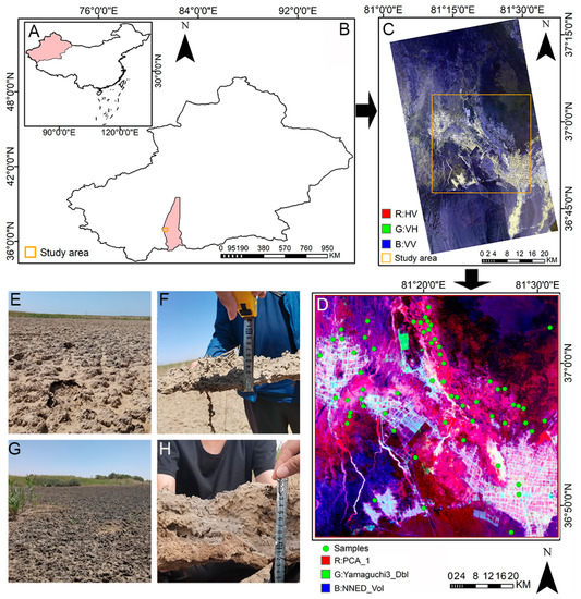
Figure 1.
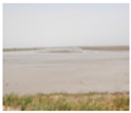
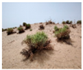
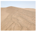
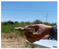
Schematic diagram of the study area. (A) The position of Xinjiang in China; (B) The location of the study area in Xinjiang; (C) PALSAR-2 image; (D) OLI + PALSAR2 image and field sampling sites; (E) Mild-moderate salty land; (F) Determination of salt shell in mild-moderate salty land; (G) Severely salty land; (H) Determination of salt shell in severely salty land.
In addition, the study area experiences a persistent shortage of water resources. The major source of water here depends on a seasonal stream, the Keriya River. Its source is glacial meltwater and snow from the Kunlun Mountains, which ultimately dries up in the gravel of the Taklimakan Desert [37,38]. Water efficiency impacts vegetation types such as xerophytes and halophytes within the study area and influences soil types, including mainly meadow soil and desert brown soil [19,39]. Soil salinization exacerbates desertification and ecological soil degradation in the Keriya Oasis, and creates an obstacle to sustainable local agriculture and ecological development. Therefore, it is meaningful to thoroughly understand the characteristics of this region and promptly monitor the spatial distribution of soil salinity.
2.2. Remote Sensing Data and Preprocessing
An observation series satellite, the ALOS-2 satellite launched by the Japan Aerospace Exploration Agency laboratory in 2014, carries a PALSAR-2 sensor [32]. In this study, PALSAR-2 data were obtained on 23 April 2015, with an angle of incidence of 30.4°. Four polarizations were achieved by combining the horizontal (H) and vertical (V) polarization modes: HH, HV, VH, and VV [40]. Data from the Landsat-8 OLI sensor used in this study was collected on 26 April 2015, with a cloud cover of 0.3%. The major parameters for remote sensing data are presented in Table 1.

Table 1.
Major parameters of remote sensing data.
The PALSAR-2 imagery was processed using PolSARpro_6.0 software from the Polarimetric SAR Data Processing and Educational Toolbox, which was developed under contract with the European Space Agency by a consortium led by the Institut d’Electronique et de Telecommunications de Rennes (Institute of Electronics and Telecommunications at Rennes) at the University of Rennes, France. The steps of processing include the following: (1) the generation of a single-look complex image; (2) the T3 polarization coherent matrix was decomposed while performing multilooking (the azimuthal vision was 8 and the range directional vision was 5); (3) speckle filtering, which was used in this module to remove coherent noise through an advanced Lee filter (with a window size of 7 × 7 pixels); (4) geocoding and radiometric calibration, which was completed based on the Universal Transverse Mercator projection; (5) the resampling of the image to a resolution of 15 m × 15 m; and (6) the creation of an image subset by selecting a suitable range as the study area from the areas common to optical and radar images. The process is shown in Figure 2.
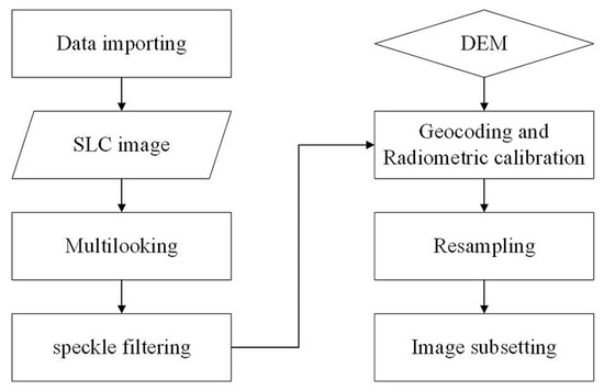
Figure 2.
Preprocessing flowchart of PALSAR-2 data.
The preprocessing of the OLI images was performed using ENVI_5.3 software, which is used to process and analyze geospatial images to extract timely, reliable, and accurate image information. It is scientifically validated, easy to use, and closely integrated with several other platforms, including radiometric calibration, atmospheric correction, image-to-map registration, resampling, and the creation of an image subset. Finally, the preprocessed OLI images had the same range and resolution as the PALSAR-2 images. In addition, online high-precision maps obtained from the OvitalMap website were chosen as the reference images for selected features (https://www.ovital.com/, accessed on 28 April 2022).
2.3. Field Data
Field surveys in this study area were conducted between 23 April to 7 May 2015. Soil samples were collected from a total of 61 sites and from areas with different degrees of soil salinity, and the information such as time, point number, and vegetation type was recorded together. Each soil sample was taken at the ground surface (0–20 cm), with the latitude and longitude of the samples recorded at the time of collection in the WGS84 coordinate system. The samples were then taken to the laboratory. Subsequently, the physical and chemical characteristics of the soil were determined in the lab. The main steps are as follows: (1) the soil samples were dried naturally in dark conditions; (2) samples were ground and filtered with 1 mm sieves; (3) soil samples of 20 g each were then obtained by weighing an electronic balance placed in a flask containing five times the weight of the soil in distilled water. The flask was sealed and the solution was shaken about 200 times; (4) the mixed solution was left for about one hour until the soil and solution had separated; (5) the filter paper was folded in half twice in succession to present a funnel shape. The solution was filtered along a glass rod from one end of the triple filter paper and the filtrate was collected. Electrical conductivity (EC) and total dissolved solids (TDS) were measured using an electrical conductivity meter (inoLab® Cond 7310, WTW, Munich, Germany), and pH was measured using a pH analysis tester (inoLab® pH 7310, WTW, Munich, Germany). Soluble salt content in a soil solution is usually positively correlated with electrical conductivity; therefore, some researchers have used conductivity to directly calculate the total salt content of soil by a regression equation [41,42,43] and this paper also took this approach. The salt content, EC, TDS, and vegetation cover were determined for the different classes of saline soils such as severely and mild–moderately salinized soil. A classification of the different degrees of salinity was obtained from 61 soil samples and their photo library, and laboratory salinity results, compared with the “Soils and Improved Use in Xinjiang” provided by the Xinjiang Institute of Biology, Soil and Desert, CAS [44]. The land cover was classified into five categories: water, vegetation, mild-moderately salinized soil, severely salinized soil, and bare land (Table 2).

Table 2.
LCLU classes with varying severity of soil salinization, characteristics, and their picture.
2.4. Polarimetric Decomposition
The design idea of this paper is shown by the flow chart in Figure 3. The goal of target polarization decomposition is to obtain ground object information about the features of different vectors by establishing a one-to-one correspondence between the scattering feature components of the image and the physical characteristics of the actual ground object [45]. Two standard methods of target polarization decomposition exist: coherent and incoherent target decomposition. The first is based on a target scattering matrix, while the second is based on other measures, such as a polarization coherence matrix. Cloude decomposition is a non-coherent objective decomposition method. This method has been proposed from the analysis of a specific vector of a polarization matrix, which was also the first time that the concept of an eigenvalue was introduced into target decomposition theory. Cloude decomposition fully uses the characteristics of the orthogonal scattering mechanism and reduces the influence of various polarization bases on objects on the ground [46]. The coherent matrix [T] can be represented by using a self-conjugate matrix:
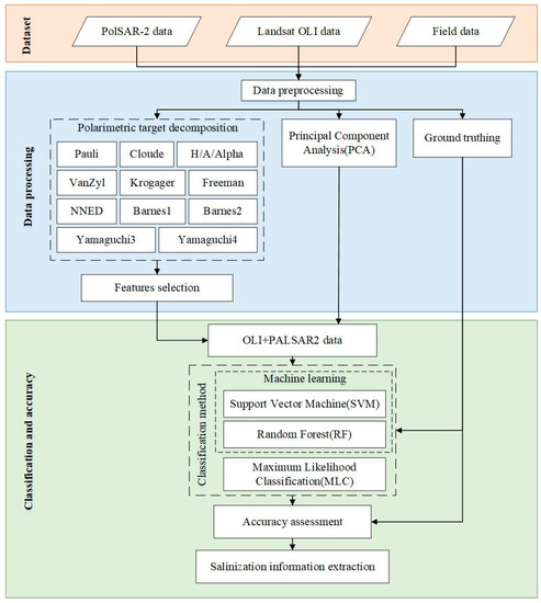
Figure 3.
The overall workflow of the study.
In Equation (1), the meaning of ⋇ is expressed as a complex conjugate transpose; [Λ] is a diagonal matrix consisting of eigenvalues [T]; the real eigenvalue is ≧ ≧ ≧ 0; [] is a generalized unitarity matrix; [T] can be decomposed into the sum of three coherent matrices [Ti] (i = 1,2,3) that are independent of each other. The decomposition for this case is:
where λi is the eigenvalue, and ei is the eigenvector. In this case, [Ti] denotes the independent coherence matrix of rank 1 and λi indicates the intensity. Cloude decomposition is not limited to a fixed scattering mechanism, so it has the characteristic of base constancy and better stability than other methods [47]. Meanwhile, T11, T22, and T33 are three characteristic parameters obtained by Cloude decomposition, representing surface, double, and volume scattering. In this paper, the 11 polarization decomposition methods used include Cloude [48], Krogager [49], Pauli [23], H/A/Alpha [50], VanZyl [51], Arii3 Component NNED [52], Freeman [22], Barnes1 [53], Barnes2 [54], Yamaguchi3 and Yamaguchi4 [55,56]. In addition, 33 polarization scattering feature components were extracted using the above methods.
Meanwhile, the feature information of OLI images was optimized using Principal Component Analysis (PCA). The principle of PCA is to transform multiple indicators into a few composites using multivariate statistical analysis to remove the redundant information among indices. Usually, a linear combination of the original indicators is used as the new composite factors, and a linear combination is ranked according to the magnitude of their variances. The most significant linear combination is called the first principal component.
2.5. Features Optimization
It is well-known that blindly selecting all characteristics for classification results in redundant data and information, while reducing classification accuracy. These two problems can be solved by selecting only the desired features [57]. Assessing the quality of an image can generally be achieved using the signal-to-noise ratio (SNR) method, which is defined as the ratio of target intensity to noise [32]. Using an SNR has the advantage of extracting components from the rich information of the images while reducing their dimensionality. When the SNR is relatively high, the image is sharper and less affected by speckle noise. Therefore, the six best feature components were extracted from the 33 features in the imagery using the SNR, which can reflect the characteristic information of soil salinization. The SNR of each characteristic feature was calculated and summarized in Table 3 and Figure 4.

Table 3.
SNR values of characteristic components.
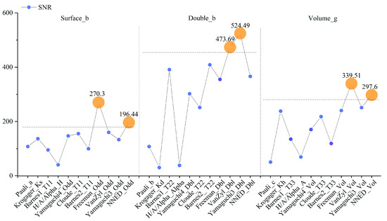
Figure 4.
Polarization feature optimization.
2.6. Construction of Machine Learning Classification Models
The classification methods used in this study include SVM, RF, and MLC. The first two methods are commonly used in machine learning, and the latter is a widely used method based on standard statistical features as a control group.
Among them, Cortes and Vapnik proposed the SVM classification method, a statistical technique that extracts the characteristics of the target and identifies the data structure as the target [58]. An SVM can show unique advantages in resolving the recognition of small sample features and higher dimensional states. It is used in an effective learning algorithm for linear classifier parameters with a massive capacity. The SVM method relies on a binary classification template. When a model has two different types of vectors, a linear decision function is determined by establishing a discriminant function that distinguishes between the two classes with maximum accuracy, which can be expressed as:
Through analysis, the study of issues of convex quadratic programming is helpful to the transformation of objectives, and there is a unique optimal solution. Using the Lagrange multiplier, the formula is:
where αi refers to the Lagrange factor. The following formula is obtained by processing, respectively:
where is the number of support vectors, and ⟨xi·x⟩ is the inner product operation. When the number of samples is limited, the SVM finds the best function by adjusting it more than once in the model. This reduces the characteristic spatial dimension and resolves the dimensional disaster, which is the strength of this model [59]. In addition, RF is a model implemented by ensemble learning that uses decision trees as the main classifier; each decision tree decides the outcome through a simple vote. The principle is to generate random samples to form subsets using the self-sampling method, where each subset comprises a decision tree, and multiple decision trees make up a random forest [60].
The three steps of MLC are [61]: (1) to determine the different types of training samples; (2) calculate the different types of statistical feature values from the training samples and establish the classification discriminating function; and (3) the classification of the image is completed by judging the class to which each pixel belongs on a per-pixel basis. The category is determined based on the maximum function value.
2.7. Classification Accuracy
This paper uses three objective evaluation metrics to appraise the classification accuracy of the classified images. They are overall accuracy (OA), a Kappa coefficient, and the F1 score [62]:
where P(i,j) represents all image pixels of category i that are assigned to the category j, and the n is the number of all categories. The value of OA ranged from 1% to 100%; the closer the value is to 100%, the better the image classification. The Kappa coefficient can be calculated using Equation (8):
As a powerful technique, Kappa can provide the information for a single matrix and count the compared matrices. In Equation (8), N refers to the total sample size, , , …, are the actual number of samples of each type, and , , …, are the predicted number of samples of each type. Kappa values range from 0–1; if the value is closer to 1, the outcome is better. In this paper, to enhance the accuracy of image classification, an extra F1 score was added, which is a standard accuracy evaluation index based on the machine learning classification, and is calculated as follows:
where the F1-score indicates precision and recall integration for a composite index; TP and FP refer to the true and false positive, respectively; TN and FN refer to a true and false negative, respectively; and F1 in Formula (11) is the harmonic means of both [63,64]. The F1 has the same range as Kappa, so the closer the score is to 1, the better the result.
3. Results
3.1. Polarimetric Decomposition of PALSAR-2 Data
Based on the PALSAR-2 image, a total of 33 scattering features were extracted using eleven polarization decomposition methods. There were mainly divided into three types, surface scattering (*_Odd), double scattering (*_Dbl), and volume scattering (*_Vol) according to the scattering type. The *_Odd mainly reflects the relatively flat characteristics of the landscape such as farmland and water surface. The *_Dbl mostly captures the information about the angle of tree trunks and the ground. Vegetation information usually shows the *_Vol type of surface scattering, which also reflects the distribution of regional salinization to some degree [65,66]. The polarization scattering features were sorted out in Table 4, and the red/green/blue (RGB) color composite diagram of polarization decomposition is presented in Figure 5 (R: *_Dbl/; B: *_Odd/; G: *_Vol).

Table 4.
Polarization decomposition methods and characteristic components.
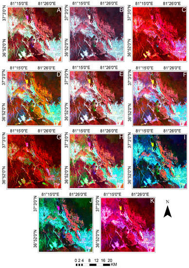
Figure 5.
Polarization decomposition. (A) Pauli; (B) Krogager; (C) Cloude; (D) H/A/Alpha; (E) VanZyl; (F) Arii 3 Component NNED; (G) Yamaguchi3; (H) Freeman; (I) Barnes1; (J) Barnes2; (K) Yamaguchi4.
3.2. Optimal Scattering Features
The 33 polarized scattering components were divided into three groups according to similar physical scattering methods; all the components in the same group were compared. The two components with the highest SNR value in the same group were selected as the optimum scatter features for that group. Finally, the six best features were chosen, including Freeman_Odd, VanZyl_Dbl, VanZyl_Vol, Yamaguchi3_Dbl, Arii 3 Component NNED_Odd, and Arii 3 Component NNED_Vol.
PCA concentrates most of the information from the OLI data in the first two bands; then PCA_1 and PCA_2 were selected as the optimal information content bands in the optical images. They combined six features of the PALSAR-2 image to form a dataset of about eight components, namely the OLI + PALSAR2 image illustrated in Figure 6I.
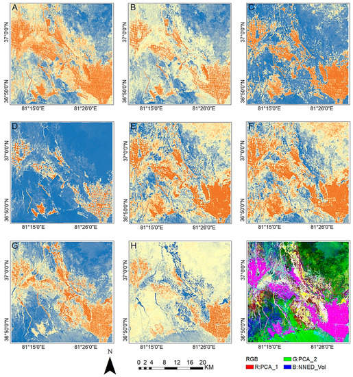
Figure 6.
Optimal component false color image. (A) Freeman_Odd; (B) NNED_Odd; (C) VanZyl_Dbl; (D) Yamaguchi3_Dbl; (E) VanZyl_Vol; (F) NNED_Vol; (G) OLI PCA_1; (H) OLI PCA_2; (I) OLI + PALSAR2 data (R: OLI PCA_1, G: OLI PCA_2, B: NNED_Vol).
Figure 6A–F indicate the six best scattering features obtained from PALSAR-2 images using the polarization decomposition method. Figure 6G,H demonstrate that the two optimal bands, PCA_1 and PCA_2, which were obtained using PCA on the OLI images. Figure 6I show the synthetic dataset of composite OLI + PALSAR2 images.
Different polarization decomposition features respond differently to various surface types. The brown area indicates vegetation, as seen from the texture and coverage presented in Figure 6. The patterns of Figure 6A,B show surface scattering, which mainly emphasizes the relatively flat surface of the soil and its distribution interspersed with vegetation. Figure 6C,D show double scattering; they primarily capture information on the angle between a tree trunk and the ground, which respond to the distribution of vegetation. Volume scattering information is mainly presented in Figure 6E,F, which can not only reflect the vegetation information but also highlight the distribution of land with an uneven surface. Figure 6G,H are supplemented with detail on various object features, such as texture, variation in color, and the ability to maintain target edges. As shown in Figure 6I, it is relatively easy to distinguish between the different targets by combining the optimal characteristics and the PALSAR-2 features. Water is associated with yellow areas. The color of the vegetated areas is mostly red, and the texture reflects the attributes of farmland. Green areas are primarily associated with different degrees of salinity, and the shade of green can be used as one of the bases for determining the degree of salinity in the soil.
3.3. Classification Results and Accuracy
The OLI, PALSAR-2, and OLI + PALSAR2 images were all classified using the SVM, RF, and MLC methods; the training and validation samples were selected based on field data, and Landsat8 OLI and OvitalMap images were used as reference images. The results of the classification can be seen in Figure 7.
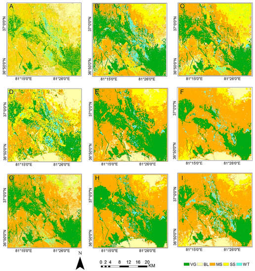
Figure 7.
Classification results. (A) RF classification of PALSAR-2 image; (B) MLC classification of PALSAR-2 image; (C) SVM classification of PALSAR-2 image; (D) RF classification of OLI image; (E) MLC classification of OLI image; (f) SVM classification of OLI image; (G) RF classification of OLI + PALSAR2 image; (H) MLC classification of OLI + PALSAR2 image; (I) SVM classification of OLI + PALSAR2 image.
According to the classification results of Figure 7, the PALSAR-2 images (Figure 7A–C) showed that the speckle noise was widespread, leading to inaccuracy in classifying objects on the ground. The OLI images (Figure 7D–F) show that vegetation, water, and mild-moderately salinized soils appeared to have a mixed distribution. The OLI + PALSAR2 results (Figure 7G–I) show that the characteristics were largely independently distributed and reduced the influence of speckle noise. Based on field survey experience, the distribution of land objects in Figure 7I was closer to the current situation. In the study area, the central vegetated area was considered the center of the oasis and its type is mainly agricultural land, and water are scattered in the area. In addition, mild-moderately salinized soil was interspersed with cultivated land and enclosed the cultivated land. The change in soil type at the edge of the desert was from mild-moderately to severely salinized soil. The level of land salinization showed a progressive upward tendency from the oasis towards the desert. The classification results were evaluated quantitatively based on measures of the OA, Kappa coefficient, and F1 score (Table 5).

Table 5.
Accuracy Evaluation.
Table 5 shows the classification results using the SVM classifier; the effect of the OLI + PALSAR2 images was relatively better, with an OA of 91.57%, Kappa of 0.89, and F1 of 0.94. When using OLI + PALSAR2 data, the OA of the SVM was increased by 17.23% and 2.02% compared to RF and MLC, respectively. Meanwhile, their Kappa were 0.70 and 0.84, respectively; these values were lower than those obtained from the OLI + PALSAR2 data. In addition, the same was true for F1, with lower results of 0.79 and 0.89, respectively. Based on the SVM classifier, the OA of OLI + PALSAR2 increased by 16.5% and 4.08% compared to the PALSAR-2 and OLI data, respectively. Also, the Kappa improved by 0.23 and 0.11, and F1 was enhanced by 0.27 and 0.10 each of them.
4. Discussion
4.1. Impact of Polarimetric Decomposition on Classification
Multiple target polarization decomposition processing of PALSAR-2 data and the extraction of scattering features reflected more information about the study area. It also established a more accurate correspondence between PALSAR-2 images and actual targets. There are primarily areas with surface, double, and volume scattering. The information on soils is captured by the surface scattering component, and for the other two components, the vegetation has a higher backscattering coefficient than the other targets. Volume scattering occurred mainly in areas with high vegetation cover, and the double scattering complements the texture information of the area to some extent, so that the soil salinization is higher in areas where there is less information on the vegetation. As well, the volume scattering highlights the desert area and captures information about the undulating dunes. Water was mainly identified by surface scattering. In addition, optical data mainly captured the reflection information of the targets with seven bands, while the spatial resolution of the sensor was limited. The PolSAR data had higher spatial resolution and different sensitivities to soil types and could compensate for the lack of optical data.
4.2. Impacts of Different Classifiers on Classification
Among the three classifiers, the SVM method provided slightly better classification results than the other two methods; the classification results improved for all three datasets. In the classification results, based on OLI + PALSAR2 data, the outcomes obtained from the RF classifier show that there is a high level of speckle noise in the images and a certain degree of confusion in the targets, with some of the resulting mild-moderately salinized soil being incorrectly identified as bare land. The reason for this result could be model over-fitting. The MLC results showed that some mild-moderately salinized soils were considered vegetation. In addition, this approach ignored independently existing targets such as small areas of reservoirs and ponds. For the SVM classifier, the overall accuracy obtained increased by 17.23% and 2.02% over RF and MLC methods, respectively. Not only were the boundaries of different types of features more effectively delineated, but targets in small areas, such as fish ponds and small areas of vegetation, were also retained. The method was also able to capture soil salinity information more accurately, independent of speckle noise to a certain extent. This shows that the SVM method based on machine learning retains feature independence in a small range and reduces misclassification by multiple iterations. For this study area, the accuracy achieved by using the SVM method to extract saline soils exceeded the results of other classifiers.
4.3. Distribution Characteristics of Salinization in the Study Area
The distribution of soil salinization in the study area shows a trend of gradual inward erosion from desert to oasis. This is caused by a combination of the local arid climate, topographical factors, and a shortage of water resources. When considering the mechanisms of salinity formation, two factors should be considered simultaneously: salt and water. The elevation of the area is lower in the south than in the north, and the water storage capacity of sandy soils is weak, so the groundwater level in the northern part of the region is shallow. This is one of the reasons for the formation of salinity zones extending from desert to oasis. When water evaporates from the ground, the salt tends to accumulate on the soil surface, and then water in the soil rises from the soil capillaries and eventually floats on the soil surface, exacerbating the salinization of the soil [26]. Most locals use diffuse irrigation in their farmland, which tends to bring salt from the soil surface back to the roots of vegetation. This leads to a circulation of salts in the soil surface and the vegetation roots, causing a staggered distribution of saline land and agricultural land, thus impeding sustainable agricultural development and negatively impacting the agricultural economy.
4.4. Potential and Limitations
This study extracted information on the distribution of soils with different levels of salinity in the Keriya Oasis from remote sensing data and field data, combined with machine learning to classify the ground targets and achieve good accuracy. Some limitations and potential factors are indicated here. It is still difficult to clearly distinguish between soils with different degrees of salinity because the response mechanisms of polarimetric scattering features are influenced by several factors, including vegetation cover, soil roughness, the dielectric constant, and soil moisture. On this basis, it is necessary to explore the quantitative relationship between the physical properties of the echoes of radar images and the surface salinity, as well as to analyze several other factors, in order to form a model that responds to soil salinity information. Another limitation is the fact that speckle noise in radar images cannot be removed entirely. This noise can be suppressed by extracting effective scattering features in a PolSAR image. However, the extraction method used in this paper is not comprehensive enough, and more authoritative metrics are needed for feature preference. Optimizing the kernel parameters and penalty parameters can exploit the potential of the SVM classifier, and these ideas can be explored in future research.
5. Conclusions
The PALSAR-2 and OLI images of the Keriya Oasis combined with polarimetric scattering features and machine learning classifiers were used to monitor saline soil distribution in arid regions. Multiple polarimetric decomposition methods (Cloude, Krogager, Pauli, H/A/Alpha, VanZyl, Arii3 Component NNED, Freeman, Barnes1, Barnes2, Yamaguchi3, and Yamaguchi4) were used to highlight soil salinity information and improve classification outcomes. The conclusions are as follows. First, the PALSAR-2 images were decomposed by 33 polarimetric scattering features that were acquired. Using SNR, six polarization scattering features were highlighted: Freeman_Odd, VanZyl_Dbl, VanZyl_Vol, Yamaguchi3_Dbl, Arii3 Component NNED_Odd, and Arii3 Component NNED_Vol. The aforementioned components could effectively complement the differences between scattering features and distinguish between different degrees of salinity information. Second, the OLI + PALSAR2 dataset was synthesized from eight excellent features, consisting of six polarized scattering features and two PCA components. The classification accuracy of the OLI + PALSAR2 image was better compared to that of the original radar or a single optical image. Compared to PALSAR-2 and OLI images, the OA of the OLI + PALSAR2 was improved by 17.23% and 2.02%, respectively, when using the SVM classification method. Third, the SVM method based on machine learning was used as a classification method to extract different degrees of salinity, and relatively good classification results were achieved. The accuracy of the OLI + PALSAR2 data combined with SVM was 91.57%.
In this paper, OLI + PALSAR2, a comprehensive dataset, is obtained by extracted polarization information from PALSAR and combined it with spectral information from OLI. In addition, the speckle noise in PALSAR data has been reduced, and the band redundancy of the optical data was reduced. Combining the advantages of two types of data improved the classification accuracy of soil salinity information by using the SVM based on the machine learning method. The classification results showed that the use of the SVM method combined with PALSAR-2 and OLI data was more suitable for monitoring the information on the distribution of different salinization degrees than other methods within this study area. The monitoring of soil salinity in this study can provide a reference for the prevention and improvement of saline soils in the study area, and provide reasonable suggestions for sustainable agricultural development and ecological environmental protection.
Author Contributions
Conceptualization, I.N. and J.Z.; methodology, I.N., N.M. and J.Z.; software, J.Z. and S.X.; validation, I.N., N.M. and A.A.; formal analysis, S.X.; investigation, J.Z., A.A.; resources, I.N.; data curation, J.Z.; writing—original draft preparation, J.Z.; writing—review and editing, I.N.; visualization, J.Z., S.X.; supervision, I.N., N.M.; project administration, I.N.; funding acquisition, I.N. All authors have read and agreed to the published version of the manuscript.
Funding
This research was funded by the National Natural Science Foundation of China [No. 42061065, and No. 41561089].
Institutional Review Board Statement
Not applicable.
Informed Consent Statement
Not applicable.
Data Availability Statement
Not applicable.
Acknowledgments
The authors thank I.N. for his involvement in the design of the study, and N.M., S.X. and A.A. for their support during the fieldwork, discussions and writing of the paper. Finally, we also extend our gratitude to the anonymous reviewers of this manuscript for their valuable suggestions during the preparation process.
Conflicts of Interest
The authors declare no conflict of interest.
References
- Jumeniyaz, S.; Lv, G.; Ilyas, N.; Tayierjiang, A.; Abdulla, A.; Mamat, S.; Abdugheni, A.; Mamattursun, E. Model Prediction of Secondary Soil Salinization in the Keriya Oasis, Northwest China. Sustainability 2018, 10, 656. [Google Scholar] [CrossRef]
- Guo, J.P.; Gao, S.H.; Liu, L. Agricultural Development and Efficient Utilization of Agroclimatic Resources in Western Region of China. Resour. Sci. 2002, 24, 22–25. [Google Scholar]
- Dehaan, R.; Taylor, G.R. Image-Derived Spectral Endmembers as Indicators of Salinisation. Int. J. Remote Sens. 2003, 24, 775–794. [Google Scholar] [CrossRef]
- Tian, C.Y.; Zhou, H.F.; Liu, G.Q. The Proposal on Control of Soil Salinizing and Agricultural Sustaining Developmentn in 21’s Century in XinJian. Arid Land Geogr. 2000, 23, 177–181. [Google Scholar]
- Ding, J.L.; Yang, S.T.; Shi, Q.; Wei, Y.; Wang, F. Using Apparent Electrical Conductivity as Indicator for Investigating Potential Spatial Variation of Soil Salinity across Seven Oases along Tarim River in Southern Xinjiang, China. Remote. Sens. 2020, 12, 2601. [Google Scholar] [CrossRef]
- Adilai, A.; Ilyas, N.; Nuerbiye, M.; Sentian, X.; Jing, Z. Monitoring of Soil Salinization in the Keriya Oasis Based on Deep Learning with PALSAR-2 and Landsat-8 Datasets. Sustainability 2022, 14, 2666. [Google Scholar] [CrossRef]
- Li, J.G.; Pu, L.J.; Zhu, M.; Zhang, R.S. The Present Situation and Hot Issues in the Salt-Affected Soil Research. Acta Geogr. Sin. 2012, 67, 1233–1245. [Google Scholar]
- Vermeulen, D.; Van Niekerk, A. Machine Learning Performance for Predicting Soil Salinity Using Different Combinations of Geomorphometric Covariates. Geoderma 2017, 299, 1–12. [Google Scholar] [CrossRef]
- Ge, X.; Ding, J.; Teng, D.; Wang, J.; Huo, T.; Jin, X.; Wang, J.; He, B.; Han, L. Updated Soil Salinity with Fine Spatial Resolution and High Accuracy: The Synergy of Sentinel-2 MSI, Environmental Covariates and Hybrid Machine Learning Approaches. CATENA 2022, 212, 106054. [Google Scholar] [CrossRef]
- Lee, J.S.; Pottier, E. Polarimetric Radar Imaging: From Basics to Applications, 1st ed.; CRC Press: Boca Raton, FL, USA, 2009; ISBN 978-1-4200-5498-9. [Google Scholar]
- Xiao, S.; Nurmemet, I.; Muhetaer, N.; Zhao, J.; Abulaiti, A. Spatial and Temporal Analysis of Soil Salinity in Yutian Oasis by Combined Optical and Radar Multi-Source Remote Sensing. Arid Zone Res. 2023, 40, 59–68. [Google Scholar] [CrossRef]
- Odipo, V.O.; Nickless, A.; Berger, C.; Baade, J.; Urbazaev, M.; Walther, C.; Schmullius, C. Assessment of Aboveground Woody Biomass Dynamics Using Terrestrial Laser Scanner and L-Band ALOS PALSAR Data in South African Savanna. Forests 2016, 7, 294. [Google Scholar] [CrossRef]
- Singh, A.N.; Kristof, S.J.; Baumgardner, M.F. Delineating Salt-Affected Soils in the Ganges Plain by Digital Analysis of Landsat Data. J. Indian Soc. Photo-Interpret. Remote Sens. 1979, 7, 35–39. [Google Scholar] [CrossRef]
- Qi, Z.; Yeh, A.G.-O.; Li, X.; Lin, Z. A Novel Algorithm for Land Use and Land Cover Classification Using RADARSAT-2 Polarimetric SAR Data. Remote Sens. Environ. 2012, 118, 21–39. [Google Scholar] [CrossRef]
- Taghadosi, M.M.; Hasanlou, M.; Eftekhari, K. Soil Salinity Mapping Using Dual-Polarized SAR Sentinel-1 Imagery. Int. J. Remote Sens. 2019, 40, 237–252. [Google Scholar] [CrossRef]
- Moran, M.; Hymer, D.; Qi, J.; Sano, E. Soil Moisture Evaluation Using Multi-Temporal Synthetic Aperture Radar (SAR) in Semiarid Rangeland. Agric. For. Meteorol. 2000, 105, 69–80. [Google Scholar] [CrossRef]
- Tripathi, A.; Tiwari, R. A Simplified Sub-Surface Soil Salinity Estimation Using Synergy of Sentinel-1 SAR and Sentinel-2 Multispectral Satellite Data, for Early Stages of Wheat Crop Growth in Rupnagar, Punjab, India. Land Degrad. Dev. 2021, 32, 3905–3919. [Google Scholar] [CrossRef]
- Yao, G.; Liu, X.Q.; Hou, W.T.; Han, Y.H.; Wang, R.; Zhang, H. Characteristics of Saline Soil in Extremely Arid Regions: A Case Study Using GF-3 and ALOS-2 Quad-Pol SAR Data in Qinghai, China. Remote Sens. 2021, 13, 417. [Google Scholar]
- Ilyas, N.; Vasit, S.; Ding, J.L.; Ümüt, H.; Abdulla, A.; Zaytungul, Y. A WFS-SVM Model for Soil Salinity Mapping in Keriya Oasis, Northwestern China Using Polarimetric Decomposition and Fully PolSAR Data. Remote Sens. 2018, 10, 598. [Google Scholar] [CrossRef]
- Fei, H. Research on Polsar Image Classification Based on Target Decomposition. Master’s Thesis, University of Electronic Science and Technology of China, Chengdu, China, 2016. [Google Scholar]
- Boerner, W.-M. Recent Advances in Extra-Wide-Band Polarimetry, Interferometry and Polarimetric Interferometry in Synthetic Aperture Remote Sensing and Its Applications. IEE Proc.-Radar Sonar Navig. 2003, 150, 113–124. [Google Scholar] [CrossRef]
- Freeman, A.; Durden, S.L. A Three-Component Scattering Model for Polarimetric SAR Data. IEEE Trans. Geosci. Remote Sens. 1998, 36, 963–973. [Google Scholar] [CrossRef]
- Cloude, S.R.; Pottier, E. A Review of Target Decomposition Theorems in Radar Polarimetry. IEEE Trans. Geosci. Remote Sens. 1996, 34, 498–518. [Google Scholar] [CrossRef]
- Liu, W.; Shi, J.C.; Wang, J.M. Applying the Decomposition Technique in Vegetated Surface to Estimate Soil Moisture by Multi-Temporal Measurements. Remote Sens. Inf. 2005, 12, 3–6. [Google Scholar]
- Guo, H.D.; Wang, C.; Liao, J.J.; Shao, Y.; Wei, C.J. Dual-frequency and Quad-polarization SAR Observations in Zhaoqing Region, China. Geocarto Int. 1995, 10, 79–85. [Google Scholar] [CrossRef]
- Deroin, J.-P.; Motti, E.; Simonin, A. A Comparison of the Potential for Using Optical and SAR Data for Geological Mapping in an Arid Region: The Atar Site, Western Sahara, Mauritania. Int. J. Remote Sens. 1998, 19, 1115–1132. [Google Scholar] [CrossRef]
- Lee, J.-S.; Grunes, M.R.; Pottier, E.; Ferro-Famil, L. Unsupervised Terrain Classification Preserving Polarimetric Scattering Characteristics. IEEE Trans. Geosci. Remote Sens. 2004, 42, 722–731. [Google Scholar] [CrossRef]
- Acar, H.; Özerdem, M.S.; Acar, E. Soil Moisture Inversion Via Semiempirical and Machine Learning Methods with Full-Polarization Radarsat-2 and Polarimetric Target Decomposition Data: A Comparative Study. IEEE Access 2020, 8, 197896–197907. [Google Scholar] [CrossRef]
- Wang, F.; Yang, S.; Ding, J.; Wei, Y.; Ge, X.; Liang, J. Environmental Sensitive Variable Optimization and Machine Learning Algorithm Using in Soil Salt Prediction at Oasis. Trans. Chin. Soc. Agric. Eng. 2018, 34, 102–110. [Google Scholar]
- Zhao, Y.; Qin, X.; Zou, H. Classification of Polarimetric SAR Image Based on Target Decomposition and SVM. Spacecr. Recovery Remote Sens. 2013, 34, 50–56. [Google Scholar]
- Xiao, Y.; Jiang, Q.; Wang, B.; Li, Y.; Liu, S.; Cui, C. Object-Oriented Fusion of RADARSAT-2 Polarimetric Synthetic Aperture Radar and HJ-1A Multispectral Data for Land-Cover Classification. J. Appl. Remote Sens. 2016, 10, 026021. [Google Scholar] [CrossRef]
- Nuerbiye, M.; Ilyas, N.; Adilai, A.; Xiao, S.T.; Zhao, J. A Quantifying Approach to Soil Salinity Based on a Radar Feature Space Model Using ALOS PALSAR-2 Data. Remote Sens. 2022, 14, 363. [Google Scholar] [CrossRef]
- Ilyas, N.; Shi, Q.D.; Abdulla, A.; Xia, N.; Wang, J.Z. Quantitative Evaluation of Soil Salinization Risk in Keriya Oasis Based on Grey Evaluation Model. Trans. CSAE 2019, 35, 176–184. [Google Scholar] [CrossRef]
- Nuerbiye, M.; Ilyas, N.; Adilai, A.; Xiao, S.T.; Zhao, J. An Efficient Approach for Inverting the Soil Salinity in Keriya Oasis, Northwestern China, Based on the Optical-Radar Feature-Space Model. Sensors 2022, 22, 7226. [Google Scholar] [CrossRef]
- Dwivedi, R.S. Monitoring and the Study of the Effects of Image Scale on Delineation of Salt-Affected Soils in the Indo-Gangetic Plains. Int. J. Remote Sens. 1992, 13, 1527–1536. [Google Scholar] [CrossRef]
- Wei, Y.L. Yutian County Annals; Xinjiang People’s Publishing House: Hotan, China, 2006. [Google Scholar]
- Lönnqvist, A.; Rauste, Y.; Molinier, M.; Häme, T. Polarimetric SAR Data in Land Cover Mapping in Boreal Zone. IEEE Trans. Geosci. Remote Sens. 2010, 48, 3652–3662. [Google Scholar] [CrossRef]
- Zaytungul, Y. Extraction of Soil Salinization Information in Yutian Oasis Based on Polarized Decomposition Information of PALSAR Data; Xinjiang University: Urumqi, China, 2018. [Google Scholar]
- Mamat, Z.; Yimit, H.; Lv, Y.H. Spatial Distributing Pattern of Salinized Soils and Their Salinity in Typical Area of Yutian Oasis. Chin. J. Soil Sci. 2013, 44, 1314–1320. [Google Scholar]
- Wang, H.Q.; Ramata, M.; Kalifa, G.; Wang, K. Soil Moisture Retrievals Using ALOS2-ScanSAR and MODIS Synergy over Tibetan Plateau. Remote Sens. Environ. 2020, 251, 112100. [Google Scholar] [CrossRef]
- Ma, G.L.; Ding, J.L.; Han, L.J.; Zhang, Z.P.; Ran, S. Digital Mapping of Soil Salinization Based on Sentinel-1 and Sentinel-2 Data Combined with Machine Learning Algorithms. Reg. Sustain. 2021, 2, 177–188. [Google Scholar] [CrossRef]
- Abdelgadir, A.; Rubab, A. Mapping Soil Salinity in Arid and Semi-Arid Regions Using Landsat 8 OLI Satellite Data. Remote Sens. Appl. Soc. Environ. 2019, 13, 415–425. [Google Scholar] [CrossRef]
- Han, L.J.; Ding, J.L.; Zhang, J.Y.; Chen, P.P.; Wang, J.Z.; Wang, Y.; Wang, J.; Ge, X.; Zhang, Z. Precipitation Events Determine the Spatiotemporal Distribution of Playa Surface Salinity in Arid Regions: Evidence from Satellite Data Fused via the Enhanced Spatial and Temporal Adaptive Reflectance Fusion Model. CATENA 2021, 206, 105546. [Google Scholar] [CrossRef]
- Xinjiang Institute of Biology, Soil and Desert, CAS. Soils and Improved Use in Xinjiang; Xinjiang People’s Publishing House: Urumqi, China, 1980. [Google Scholar]
- Zhao, Q.H.; Xie, K.L.; Wang, G.H.; Li, Y. Land Cover Classification of Polarimetric SAR with Fully Convolution Network and Conditional Random Field. Acta Geod. Cartogr. Sin. 2020, 49, 65–78. [Google Scholar]
- Shen, L. Research on Polarimetric SAR Image Classification Using Multifeatures Combination of Best Choice. Master’s Thesis, Liaoning Technical University, Fuxin, China, 2016. [Google Scholar]
- Jiang, Y.; Zhang, X.L.; Shi, J. A Study on Classification of Polarimetric SAR Image by Target Decomposition and Support Vector Machines. J. Image Graph. 2008, 13, 1512–1516. [Google Scholar]
- Cloude, S.R. Target Decomposition Theorems in Radar Scattering. Electron. Lett. 1985, 21, 22–24. [Google Scholar] [CrossRef]
- Krogager, E. New Decomposition of the Radar Target Scattering Matrix. Electron. Lett. 1990, 26, 1525–1527. [Google Scholar] [CrossRef]
- Cloude, S.R.; Pottier, E. An Entropy Based Classification Scheme for Land Applications of Polarimetric SAR. IEEE Trans. Geosci. Remote Sens. 1997, 35, 68–78. [Google Scholar] [CrossRef]
- VanZyl, J.J. Application of Cloude’s Target Decomposition Theorem to Polarimetric Imaging Radar Data. In Proceedings of the Optics & Photonics, San Diego, CA, USA, 12 February 1993. [Google Scholar]
- Hajnsek, I.; Pottier, E.; Cloude, S.R. Inversion of Surface Parameters from Polarimetric SAR. IEEE Trans. Geosci. Remote Sens. 2003, 41, 727–744. [Google Scholar] [CrossRef]
- Bombrun, L.; Vasile, G.; Gay, M.; Ovarlez, J.P.; Pascal, F. Roll Invariant Target Detection Based on PolSAR Clutter Models. In Proceedings of the 2010 IEEE International Geoscience and Remote Sensing Symposium, Honolulu, HI, USA, 25–30 July 2010; pp. 2511–2514. [Google Scholar]
- Holm, W.A.; Barnes, R.M. On Radar Polarization Mixed Target State Decomposition Techniques. In Proceedings of the 1988 IEEE National Radar Conference, Ann Arbor, MI, USA, 20–21 April 1988; pp. 249–254. [Google Scholar]
- Yamaguchi, Y.; Moriyama, T.; Ishido, M.; Yamada, H. Four-Component Scattering Model for Polarimetric SAR Image Decomposition. IEEE Trans. Geosci. Remote Sens. 2005, 43, 1699–1706. [Google Scholar] [CrossRef]
- Yamaguchi, Y.; Sato, A.; Sato, R.; Yamada, H.; Boerner, W.M. Four-Component Scattering Power Decomposition with Rotation of Coherency Matrix. In Proceedings of the 2010 IEEE International Geoscience and Remote Sensing Symposium, Honolulu, HI, USA, 25–30 July 2010; pp. 1327–1330. [Google Scholar]
- He, C.L.Q.; Cheng, B.; Chen, J.F.; Zhang, X.P. Information Extraction Methods of Coastal Wetland Based on GF—3 Fully Polarimetric SAR Data. Remote Sens. Nat. Resour. 2021, 33, 105–110. [Google Scholar]
- Cortes, C.; Vapnik, V.N. Support-Vector Networks. Mach. Learn. 1995, 20, 273–297. [Google Scholar] [CrossRef]
- Chi, T.; Cao, G.P.; Li, B.C.; Zikl, A.; Wang, W.L. Soil Salinity Inversion Based on Hyperspectral Data and SVM Method. J. Shandong Agric. Univ. (Nat. Sci. Ed.) 2018, 49, 585–590. [Google Scholar]
- Du, P.J.; Samat, A.; Waske, B.; Liu, S.C.; Li, Z.H. Random Forest and Rotation Forest for Fully Polarized SAR Image Classification Using Polarimetric and Spatial Features. ISPRS J. Photogramm. Remote Sens. 2015, 105, 38–53. [Google Scholar] [CrossRef]
- Gao, K.; Wang, Z.W. Extraction Method of Forest and Cultivated Land Based on GF-2 Data. Ind. Control Comput. 2020, 33, 80–81. [Google Scholar]
- Yang, S.T. Research on Crop Classification Algorithms Based on Deep Learning Using High-Resolution Remote Sensing Imagery. Master’s Thesis, Jilin University, Changchun, China, 2021. [Google Scholar]
- Cyril, G.; Eric, G. A Probabilistic Interpretation of Precision, Recall and F-Score, with Implication for Evaluation. In Proceedings of the Advances in Information Retrieval; David, E.L., Juan, M.F.L., Eds.; Springer: Berlin/Heidelberg, Germany, 2005; pp. 345–359. [Google Scholar]
- Sokolova, M.; Nathalie, J.; Stan, S. Beyond Accuracy, F-Score and ROC: A Family of Discriminant Measures for Performance Evaluation. In Proceedings of the AI 2006: Advances in Artificial Intelligence; Abdul, S., Kang, B.H., Eds.; Springer: Berlin/Heidelberg, Germany, 2006; pp. 1015–1021. [Google Scholar]
- He, C.; Xia, G.S.; Sun, H. SAR Images Classification Method Based on Dempster-Shafer Theory and Kernel Estimate. J. Syst. Eng. Electron. 2007, 18, 210–216. [Google Scholar] [CrossRef]
- Ding, J.L.; Yao, Y.; Wang, F. Detecting Soil Salinization in Arid Regions Using Spectral Feature Space Derived from Remote Sensing Data. Acta Ecol. Sin. 2014, 34, 4620–4631. [Google Scholar]
Disclaimer/Publisher’s Note: The statements, opinions and data contained in all publications are solely those of the individual author(s) and contributor(s) and not of MDPI and/or the editor(s). MDPI and/or the editor(s) disclaim responsibility for any injury to people or property resulting from any ideas, methods, instructions or products referred to in the content. |
© 2023 by the authors. Licensee MDPI, Basel, Switzerland. This article is an open access article distributed under the terms and conditions of the Creative Commons Attribution (CC BY) license (https://creativecommons.org/licenses/by/4.0/).
