Abstract
Long-term spatiotemporal Land Use and Land Cover (LULC) analysis is an objective tool for assessing patterns of sustainable development (SD). The basic purpose of this research is to define the Driving Mechanisms (DM) and assess the trend of SD in the Burabay district (Kazakhstan), which includes a city, an agro-industrial complex, and a national natural park, based on the integrated use of spatiotemporal data (STD), economic, environmental, and social (EES) indicators. The research was performed on the GEE platform using Landsat and Random Forest. The DM were studied by Multiple Linear Regression and Principal Component Analysis. SD trend was assessed through sequential transformations, aggregations, and integrations of 36 original STD and EES indicators. The overall classification accuracy was 0.85–0.97. Over the past 23 years, pasture area has changed the most (−16.69%), followed by arable land (+14.72%), forest area increased slightly (+1.81%), and built-up land—only +0.16%. The DM of development of the AOI are mainly economic components. There has been a noticeable drop in the development growth of the study area in 2021, which is apparently a consequence of the COVID-19. The upshots of the research can serve as a foundation for evaluating SD and LULC policy.
1. Introduction
The adoption in 2015 of two international action lines, such as SDG 2030 and the Paris Climate Agreement [1], contributed to a change in the trajectory of the research methodology in the area of sustainable land use apply remote sensing (RS). Thus, in the works until 2015, aimed at assessing sustainability (AS), environmental topics mainly dominated, considering the application of monomeric or individual biophysical indicators. However, in recent years, especially since 2015, the trend towards a polymer approach has become the benchmark for discussion of AS. At the same time, the basis for the integration of multidimensional indicators of, economic, environmental, social and political (EESP) nature is modern spatiotemporal data (STD) obtained using RS [2]. The second approach is quite understandable, since land use is formed under the influence of two sets of forces—human needs, as well as processes and phenomena occurring in the environment [3]. Historically, people have modified the land to obtain everything necessary for their survival or to satisfy their socio-economic, moral, and political needs [4]. At the same time, human impact on land use is due to two clusters—production and consumer activities. The production process is mainly the flow of energy and materials through the processes of extraction, processing, use and disposal of resources in the industrial and agricultural sectors. By monitoring changes in production processes in space and time, they can be made more manageable [3], while at the same time, regulation of natural processors is much more difficult.
Spatiotemporal observations alone cannot give a complete AS, since industrial and consumer activities are integral to the EESP of the well-being of the population in the territory where this is performed. In the directing of the elaboration of the STD themselves for studying the land cover based on RS, several products with spatial resolutions from 1 km to several meters have been created, which are available for free viewing [5,6]. Each of them has their own goals and objectives for which they were created, as well as restrictions on the duration of the presentation by year. An important trend is to ameliorate the precision, of the extensional resolution of these products as the technical characteristics of remote sensing satellites improve. Representing a great value for AS, these products are not without some shortcomings, which are revealed in the course of a critical analysis of their applicability for a particular purpose [7,8,9]. In addition, all these solutions require their addition with the data that are necessary for a multidimensional assessment of the development of a particular territory. These Areas of interest (AOI) can be cities, rural areas, natural parks, suburban landscapes, etc., or combinations thereof, whose land-use changes are reasoned by the anthropogenic and natal agencies. Therefore, the third degree of difficulty for AS is to conduct a multidimensional analysis of spatiotemporal and EESP parameters in areas where objects with several areas of human activity are present at the same time, where an assessment of the change in the development of each of them often deserves independent consideration. However, the object of our study Burabay district is a unique territory, which consists of a city, a national natural park (NNP) and a developed agro-industrial complex (AIC). Therefore, conceptually, our study is simultaneously tied to these three important factors (Figure 1), and the areas occupied by the city, NNP, and AIC are shown in Figure 2.
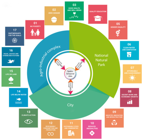
Figure 1.
The concept of the study of the Burabay district, based on the tri-unity of the city, AIC and NNP with the aim of assessing its development in the direction of SDGs.
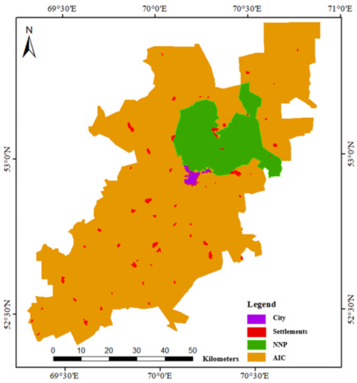
Figure 2.
The areas occupied by the city, NNP, and AIC.
In this regard, the most attention is paid to AS cities [10,11,12,13,14], since it is their expansion to other types of land use in the world, due to population growth and other factors, that often causes many negative phenomena, where ill-considered changes in LULC lead to unsustainable development of EESP conditions, the cities themselves and the territories attached to them [15,16]. AS studies of cities using RS EESP and the most advanced area where comprehensive experimental work and discussions are actively continuing [17,18,19,20,21,22,23,24,25].
Currently, there are strong epistemological tensions among researchers regarding the use of modern concepts and paradigms to assess urban development. For example, an analysis of the opinions of researchers in this direction made it possible to substantiate the importance of four approaches to assessing the development of cities: sustainability, resilience, transformation, and adaptation [26]. It is quite natural that these concepts are subject to further concretization and require clear and precise definitions. At the same time, the results of studies based on the application of the adaptation strategies, checks the resilience in combination with different forecasting models are quite interesting [27,28,29], which help to create a conceptual framework for achieving the SDGs.
As a rule, a suburban area or a rural area close to cities is considered from the point of see of the influence of a townish agglomeration, megacities, and other urban formations [13,30,31]. This process also receives a lot of attention from researchers who consider spatial and temporal changes in agriculture in direct connection and in the context of one or more EESA indicators [32,33,34,35,36,37,38,39,40,41].
The work [24] utilized a bibliometric investigation of 110 cited sciential works issued in the period from 2002 to 2022 on the assessment of sustained rural progress. The results exhibited that researchers are focusing more on methods for assessing the impact of agriculture in terms of EES parameters. They concluded that research on agrarian advancement appraisal is still juvenile, therefore, there is great potential for improvement of these problems.
The planet has a continuous trend towards the loss of biodiversity, the consequence of which from a paleontological point of view is presented as the “Sixth Mass Extinction” [42], since from their point of view, the critical point is the loss of ¾ species by the Earth living organisms. Based on this, national parks and protected areas make an invaluable contribution to improving the status of the native milieu of the planet. For example, only in Kazakhstan there are 116 such objects [43], one of which is the Burabay NNP, designed to overcome the growing crisis to achieve SDGs in the republic. NNP and forests, in addition to restoring the biodiversity of ecosystems, contribute to mitigation of the consequences of climate change, food security, and also cover both social and economic, environmental and cultural SDGs—1–7, 12, 13, 15, 17 [44,45,46,47,48,49,50].
Thus, it becomes obvious that the integration of the STD obtained based on RS and statistical data will be of key importance for achieving the SDGs [51]. This, apparently, equally applies to the city, the agro-industrial complex, and national natural parks. At the corresponding time, the methods used to quantify land-use modification based on an integrated assessment are yet under intense exploration and challenge scientific dispute [24,51,52]. At the same time, the collection of long-term STDs, their classification and analysis are greatly facilitated using the Google Earth Engine (GEE) cloud platform [8,53,54]. Involvement of the already available land cover products of different scales [5,6], because of their comparison and merging with the own data of the STD, allows a more objective approach to the assessment and analysis of land use on specific AOIs. If there is an established system for the publication of statistical information by state bodies, it becomes possible to analyze the changes found in the composition of the Land Use/Land Cover (LULC) together with the EESP factors caused by production and other human activities to assess the trend of ongoing processes.
Based on the uniqueness of the three objects located on the territory of the Burabay district, as well as considering the above features of the current areas of discussion for AS, in this work the area of research includes:
- Identification of net change of individual LULC classes with a preliminary study of some of the most effective methods for classifying satellite images, known land cover products to verify the exactness of the outcomes and the possibility of merging heterogeneous remote sensing images.
- Determination of the internal nature of land use changes: whether these processes are random or systemic, what is the intensity of the exchange between land categories and how sustainable they are.
- Calculation of multiple linear correlation between individual land classes and significant external EES statistical data to establish the most stable land use trends in the AOI.
- Study of the driving forces that contribute to the development of the area relying on the PCA method.
- Evaluation of the development tendency of the area based on a four-stage analysis of the totality of the STD and EES of statistical information.
2. Materials and Methods
2.1. Study Area
The object of research Burabay district of Akmola oblast is placed (52°23′–53°25′ N; 69°18′–70°12′ E) in the north of Kazakhstan (Figure 3).
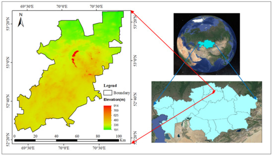
Figure 3.
Location and topography (SRTM3) of Burabay district.
The cumulative territory of the study area is 5945 km2, and the population is 73,757 people [55]. Burabay district includes 1 city, 11 administrative units subordinate to the district (Figure 4).
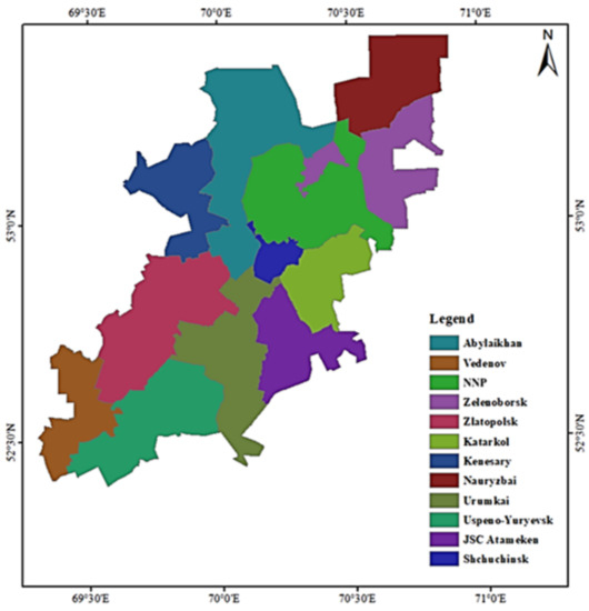
Figure 4.
Administrative units of Burabay district.
The peculiarities of the district are the presence in it of a mountain, developed agriculture, a small city, a state national natural park, a resort area and 14 lakes, which has an impact in directing the activities of the population and industrial structures of the district. Geomorphologically, the territory belongs to the northern outskirts of the Central Kazakhstan upland. The relief of this territory is a complex combination of hills and plains, crossed by a rare network of river valleys and relatively shallow lake basins.
The water level in the lakes of the district is constantly fluctuating. All lakes are characterized by the alternation of long periods of drying up and flooding. The air temperature in the region in summer and winter can vary from below −30 °C to more than +30 °C. Precipitation, depending on the height above sea level, falls from 250 to 400 mm. Favorable months for growing crops common here are the period from May to September.
The medium relative humidity of the air is 50%. The coldest month is January, the absolute maximum is −30 °C, the average January temperature is −17–18 °C. The nature of the distribution of average monthly precipitation, temperature and wind regimes over a long-term period is relatively stable, which is due to the barrier effect of the geological structure of the territory [56].
2.2. Data Sets
In this research, Landsat, Suomi NPP VIIRS, DMSP-OLS and NPP VIRS images were used as input data, which respectively served to obtain long-term series of “land changes” (Landsat), changes in night light time Suomi NPP VIIRS, DMSP-OLS) and changes in meteorological parameters (precipitation—Terra, surface temperatures—Landsat) [57,58,59,60,61,62,63,64,65,66]. Some characteristics of the parameters of the Satellites and Data Sets we used are shown in Table 1.

Table 1.
Characteristics of some parameters of Satellites and Data Sets.
All analytical work with remote sensing images was performed by using the GEE platform [63]. When working in GEE, we used the median value of the composite in the range for June-July. In addition, the EVI, NDVI, and NDWI indices [67,68,69,70] were used to improve the classification accuracy, SRTM3 [71] to improve the recognition accuracy, and assembled information about the socio-economic and environmental state of the district for each year of research [72,73].
2.3. Mapping Methods
2.3.1. General Methodical Approach
The general methodical approach may be shared in six phases (Figure 5).

Figure 5.
Technical flowchart of LULC mapping, driving mechanism analysis and assessing sustainable development of Burabay district.
A1. By comparing pixels from Dynamic World (2016–2021) [74], World cover (v.2 2021) [75] and Planet (2021) [76], we obtained reliable training samples.
A2. Using the above satellite images and indices, we obtained the mosaics of the Burabay region from 1999 to 2021. On the basis of “time series stability” [70,71], we selected sample points and deployed Random Forest (RF) models to educate and verify example dots.
A3. We divided sample points into 2 parts and considered 2/3 of them as training points. Then we used the RF model to the yearly synthetic satellite images dataset and to produce LULC maps. The rest 1/3 of the sample points were used to validate classification results and to calculate the model’s accuracy.
The rest 1/3 of the sample dots were applied to affirm classification outputs and to calculate the model’s accuracy.
A4. With the help of the transfer matrix, the values of net change, swap, persistence, gain, and loss, as well as the ratio of absolute change, gain, and loss to persistence were determined. Next, we determined what character (random or systematic) these processes are.
A5. Based on demographic, economic, social, and environmental factors and climate change, we conducted a principal component analysis. The method of multiple linear regression was used to quantify the contribution of each of the above factors.
A6. The AS trend of the area of interest (AOI) is based on the calculation of a a comprehensive integral index of SD [1]. Information on individual indicators has only been collected since 2010. For previous years, the information was fragmentary and did not fully include the initial indicators of interest to us.
2.3.2. Preparation of STD and Construction of Sample Data Set
The production of a time series of satellite images from 1999 to 2021 was performed on GEE the platform using unclouded samples for the vegetation period. The LULC classification is based on the ESA Global Land Cover system [77]. The major types of LULC in the Burabay district were crop land (CL), pastures (PE), forests (FT), water bodies WB, and urbanized lands (BU). Therefore, we focused only on these five types of LULC (Table 2).
Table 2.
The category of LULC in Burabay district.
An entire 2000 sample points were developed in this research: 70%—training and 30%—validation dots. The number of training and validation dots for each LULC category is shown in Table 3 and Figure 6 shows the allocation of some of the example points in the Burabay district.
Table 3.
Number of training and validation dots for each LULC category.
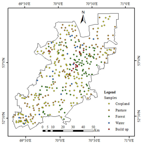
Figure 6.
Allocation of example points in the Burabay district.
2.3.3. LULC Classification Methods
To successfully classify LULC on the GEE platform, we tested three algorithms: RF, CART and SVM. The objectivity of the performed LULC classification based on Landsat 5/7/8 images using RF was checked by us using three sources: the first is comparisons with World cover data, v2, 2021 [75]; the second is LULC classification using Sentinel 2 images (spatial resolution 10 m) from 2016 to 2021 [74], using the same algorithm as for Landsat 5/7/8 (RF); and third, comparison with actual Planet images [76] (spatial resolution 6 m). In general, all three sources showed the high objectivity of our LULC classification of the Burabay district from 1999 to 2021.
2.3.4. Assessment of Land Change Exactness, Random and Systematic Transitions
When assessing the accuracy of the LULC classification from 1999 to 2021, we followed the Practical Guide proposed by the FAO [78] through the confusion matrix method. The study of the internal mechanisms of the transition of different classes of each other was carried out according to the methods described in [79,80,81].
2.3.5. PCA and MLR Model
For investigating the driving forces of AOI we took 36 demographic, social, economic, environmental, and climatic indicators (Table 4).
Table 4.
Initial indicators used in the PCA for evaluation of development Burabay district.
Principal component analysis (PCA) [82] was applied to filter out unwanted variables or noise and was executed by using IBM SPSS Statistics 26.0.
Multiple linear regression determines the level of dependence of two or more independent variables [83] and it was also carried out by supporting IBM SPSS Statistics 26.0 software.
2.3.6. Assessment of Development of Burabay District
The method for AS of the Burabay district is based on the calculation of a comprehensive integral index [1] of sustainable development, which were conventionally grouped into five groups. Information on individual indicators has only been collected since 2010. For previous years, the information was fragmentary and did not fully include the initial indicators of interest to us.
The method of evaluation includes four successive stages. The first stage is to collect the individual initial indexes. For this purpose, we selected 36 individual indicators that were combined into five groups: demographic (5), economic (10), social (9), environmental (8), and climatic (4).
The second stage is to bring heterogeneous indicators to values in the range from 0 to 100. The indicators were evaluated according to the following formula:
were,
- xij—i-value of the j-indicator,
- ximax, xjmin—the high and low meaning of the j-index indicator,
—arithmetic mean value of the j-indicator.
At the third stage, individual indicators are included in the complex in areas, such as the economy, climate, etc., which are important for determining sustainable development.
The last stage is the integration of all indicators by years to determine the general development trend over many years.
3. Results
3.1. Choice of LULC Classification Method
To choose a method for classifying LULC we compared three algorithms: RF, SVM and CART to 2021 Landsat data. As can be seen from Table 5, we did not find a significant difference between the compared classification algorithms. Therefore, given the wide distribution and relative reliability, all further work on the classification of LULC continued with the help of the RF algorithm.
Table 5.
Comparison of different methods for classifying LULC.
3.2. Accuracy Assessment of Mapping Results
At the beginning of the exploration, with the support of the GEE, a data set on LULC of the Burabay district for 1999–2021 was obtained (Table 6). The general exactness of this kit data 0.92 ± 0.044; Kappa 0.89 ± 0.05; User’s accuracy (UA) 0.94 ± 0.03; Producer’s accuracy (PA) 0.94 ± 0.03.
Table 6.
Estimating the accuracy of various LULC datasets from 1999 to 2021.
For individual classes of LULC (Table 7) from 1999 to 2021 accuracy of users and accuracy of producers, FT (0.97 ± 0.005; 0.99 ± 0.01), WB (0.99 ± 0.01; 0.94 ± 0.08) and BU (0.94 ± 0.01 0.08) were relatively high (0.99 ± 0.02; 0.99 ± 0.03), but these figures for CL (0.87 ± 0.09; 0.88 ± 0.09) and PE were relatively low (0.86 ± 0.06; 0.87 ± 0.08).
Table 7.
Accuracy assessment of different LULC types.
The outcome (Table 6 and Table 7) shows that the classification accuracy of FT, WB, and BU was lofty, which can be due to the inculcation of complementary data such as nighttime light products (NTL), DEM, EVI, NDVI, and NDWI in this research.
In contrast to WB and BU, the accuracy of the classification of CL and FT is relatively low, which can be easily seen from the changes in Confusion matrices of image data for 1999 and 2021 (Table 8).
Table 8.
Confusion matrices of image data for 1999 and 2021.
3.3. Spatial Distribution and Dynamic Changes
In general, from 1999 to 2021 (Appendix A), CL and PE were the main types in the Burabay district (Figure 7). By 2021 (Figure 8), PE had a considerable space (44.52%), followed by CL (35.40%), FT (15.96%), WB (3.05%), and the limited territory was artificial transformation land—only 1.07%.
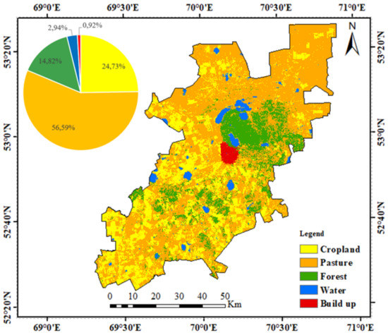
Figure 7.
LULC map of Burabay district in 1999.
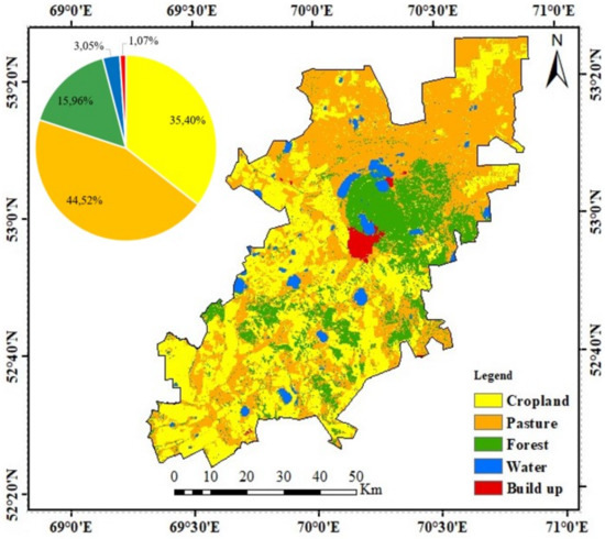
Figure 8.
LULC map of Burabay district in 2021.
Spatially CL and PE are mainly concentrated on the plains, FT are most common in hilly areas, water bodies are found in all parts of the region, BU is distributed sporadically, and the largest of them (the city of Shuchinsk and of Burabay in the region of Mount Burabay, which is clearly visible from the night image of the territory of 2021 (Figure 9 and Appendix B).
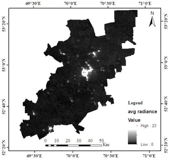
Figure 9.
Night image of the Burabay district (2021).
In the period 1999–2021 in the AOI, there was a tendency to grow the territory of CL, FT, and BU areas (Figure 10 and Figure 11). PE have been shrinking from year to year. The space of water objects over the time of the study changed little, and relatively small deviations in the size of the water surface are apparently associated with seasonal phenomena. At the same time, a sharp magnification in the part of CL and a reduction in the part of PE was noted between 2014 and 2017.
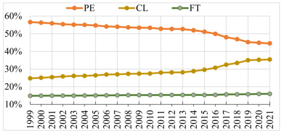
Figure 10.
Trends in different types of LULC (CL, PE, and FT) from 1999 to 2021.
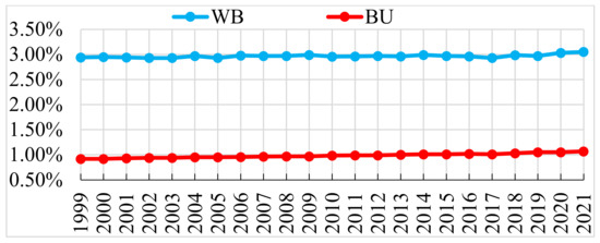
Figure 11.
Trends in different types of LULC (WB ad BU) from 1999 to 2021.
Table 9 summarizes the total change, persistence, gain, loss, exchange, net change of each LULC class between 1999 and 2021. During the observation period, a noticeable gain was experienced by CL (17.2%), moderate values of this indicator are typical for PE (8.05%) and FT (6.13%), and the minimum for BU areas (0.75%) and WB (0.31%). The greatest losses were suffered by PE (22.54%), CL are in second place in terms of losses (7.18%), and FT are in third (2.16%). The loss rates for WB (0.32%) and BU (0.22%) are negligible. The ratio of profit to loss for CL was 2.39, for FT—2.84 and for BU—3.41 times, which indicates that the increase in these LULC classes exceeded the losses.
Table 9.
Transition matrix of LULC classes (%).
The ratio of loss to profit was noted in PE (−14.49%), which indicates that the loss in this LULC class exceeded the gain. Changes in the LULC classes CL, PE, FT, WB, and BU include both swap (respectively 14.37%; 16.1%; 4.32%; 0.62%; 0.44%) and net (respectively −9.99%; 14.49%; −3.97%; 0.01%; −0.54%) change.
The percentage of various LULC classes that were immobile from 1999 to 2021 is shown on the diagonal of Table 10.
Table 10.
LULC change matrix between 1999 and 2021, %.
PE (36.9%) is the largest area of fixed land, followed by CL (17.5%) and FT (9.9%). The minimum values of land persistence to changes are typical for the WB (2.5%) and BU (0.7%) classes.
The loss to persistence ratio, i.e., Lp = loss/persistence, evaluates the liability of LULC types to changeover. Lp values over 1 point have a more intention for LULC classes to move to another type than is retained. In Table 11, Lp for all land classes below 1, generally indicates a relatively low commitment of LULC classes to transition to different land classes.
Table 11.
Ratios of gain, loss, and net change to the persistence.
It is noteworthy that the ratio of growth to persistence, i.e., Gp = gain/persistence, is not the same for all LULC classes, pointing out that individual land types have experienced more gain than persistence. For example, BU (1.05) and CL (0.98) are relatively larger Gp values, or these LULC classes are characterized by the largest land growth. The ratio of net change to persistence—Np, defined as Np = Gp − Lp, is negative for only PE (−0.57), which indicates the maximum loss of this land class during the study period.
3.4. Detecting Systematical and Occasional Conversions
The non-diagonal values of Table 12 present the growth in land class for a given steadiness if the change processes were occasional. The figures were received by allocation of the growth in each column in accordance with the fraction of other classes in 1999. he distinction between observable fractions (Table 10) and anticipated fractions (Table 12A) is presented in Table 12B. If the numerals in Table 12B are nearby to zero, the transition is closer to occasional, and if the numerals are above zero, then the transition is more systematical. The distinction between the observable and anticipated growth in the accidental process of changing pasture transition is 2.77%. Thus, the transition of 17.5% of PE to CL was caused by systematic processes of change. This means that when CL increases, new CL is usually systematically removed from PE. Differences between observed and expected benefits for transitions between CL and FT are negative (−2.16%). This means that when CL increases, new CL systematically avoids the increase due to FT areas. In other happenings, the distinction between observable and anticipated transition benefits was relatively small.
Table 12.
Intercategorical gains.
The expected losses for the random loss process are shown in Table 13A, while distinction between observable and anticipate losses are shown in Table 13B.
Table 13.
Intercategorical losses.
Thus, the simultaneous manifestation of systematical benefits and losses (Table 12B and Table 13B) shows that the major prepotent signals of modification are the transformation of PE to CL and FT. These transitions are shown in Figure 12 and Figure 13, from which it is easy to see that systematic transitions are mainly characteristic of the CL and PE classes (Figure 12).
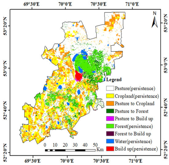
Figure 12.
Systematic land transitions of different LULC classes.
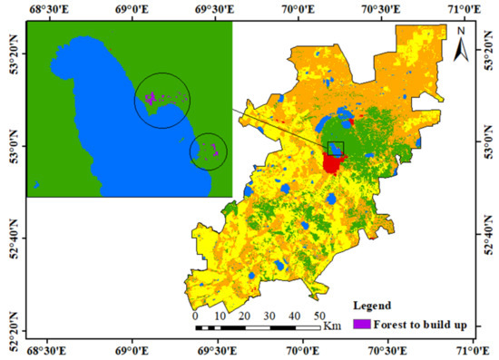
Figure 13.
An example of a random transition from a FT to a BU class.
The distinction between observable and anticipated losses because of the random loss process for PE-CL is 10.67, which means that PE systematically gives way to CL. The difference distinction between observable and anticipated losses during the transition between CL-PE and FT-PE is significant and negative (respectively −7.29 and −5.35). This shows that CL and FT systematically avoided losses to PE. In other words, PE systematically gave way to CL, and CL and FT systematically avoided losing land to PE.
Random transitions, as a rule, occupied small areas, so we have only one enlarged image showing the seizure of land from the FT for development (Figure 13).
The magnification in CL leads to a growth in gross output and improves the economic situation. The growth of the FT area increases the absorption of carbon in the ecosystem and acts a significant role in stabilizing the ecological situation in this unique territory, one of the functions of which is the organization of recreation and treatment for people.
3.5. Analysis of Driving Mechanisms
PCA was used to find the driving forces for sustainable land use. An analysis of the principal components showed that out of 36 initial indicators, only 12 falls into the composition of F1 and F2 (Table 14), while the rest of the studied characteristics did not have significant values and belong to the category of noise.
Table 14.
PCA’s rotated component matrix.
The prime main component (F1) is a characteristic of economic growth, mostly reverberating modifications in the volume of agricultural production (X1), Average monthly wages (X2), number of rural settlements with centralized water supply (X3), number of business entities (X3), Fixed capital investment (X5) and gross output (X6). The other principal component (F2) is the values of the EVI (X7), NDVI (X8), and NDWI (X9) indices and the characteristics of local climate change, reflecting the total amount of summer precipitation (X10), the total annual amount of precipitation (X11) and the temperature of the vegetation period (X12). Some examples of precipitation and temperature changes based on RS for the AOI are shown in Figure 14 and Figure 15, and the rest are in Appendix C and Appendix D.
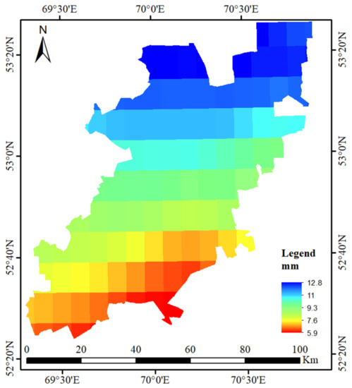
Figure 14.
Example of changes in precipitation for June 2021 in Burabay district.
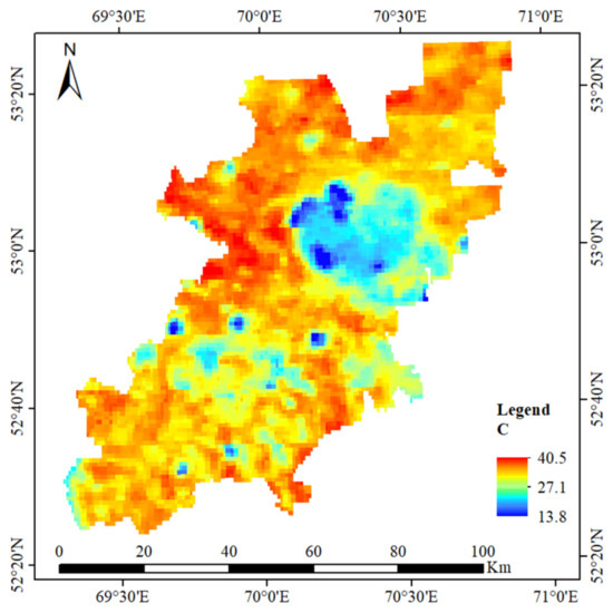
Figure 15.
Example of changes in temperature for June 2021 in Burabay district.
With the help of multiple linear regression analysis, it is possible to obtain a model of the statistical relations betwixt the change in land space and the main components of driving factors (Table 15).
Table 15.
Relationship between changing LULC classes and principal components.
Amongst them, the relationship models of CL, PE, FT, and artificial transformation confirmed the importance test, while the model of the relationship of drivers of change in the area of WB did not pass the importance test. Concrete models are next:
- -
- the field of CL, FT, and BU areas is positively associated with economic development (F1) and negatively with changes in the EVI, NDV, NDWI, and climate indices (F2). This means that with a magnification in the space of CL of FT and BU areas in the study area, economic performance improves;
- -
- PE areas are negatively associated with economic indicators (F1) and positively with changes in the EVI, NDV, NDWI and climate indices (F2). That is, a decrease in PE areas tends to lead to a decrease in economic indicators, but this is not happening yet due to the high economic efficiency of CL use.
- -
- the correlation between changes in the space of WB with the components F1 and F2 turned out to be minor (R2 = 0.46) and, apparently, these relations do not execute a serious part in the rise of the economic characteristics of the area.
In general, the driving forces for the development of the region are economic indicators such as the volume of production, investments, etc., which is logically justified and convincingly proven by the data in Table 14.
3.6. Sustainability Assessment
Group indicators of sustainable development of the Burabay district from 2010 to 2021 are presented in Table 16.
Table 16.
Group indicators of sustainable development of the Burabay district 2010–2021.
The demographic situation in the AOI, with the relative stability of the quantity of people, is characterized by the growth of townish residents over the rural population. In principle, this situation is typical for many countries of the world, and, apparently, the Burabay district is no exception in this process.
The demographic situation in the AOI, with the relative stability of the amount of people, is characterized by the growth of townish residents over the rural population.
The computations testify to the affirmative dynamics of the economic indicators of the Burabay district. This is due to considerable growth in agricultural production and investment in fixed assets in agriculture. So, from 2010 until 2021 the region increased: the size of manufacturing by 4.4 times, investments in fixed assets by 2.6 times, and gross output by 1.9 times. The performed calculations testify to the affirmative dynamics of the economic indicators of the AOI.
In the social sphere, there has been an improvement in such indicators as the “Number of rural settlements with centralized water supply”, “average monthly wages”, “decrease in unemployment”, and “the number of preschool institutions and children in them”.
Over the years of the study, the average salary of the residents of the district increased by 2.8 times, the number of rural settlements with centralized water supply—by 1.3 times, and the number of preschool institutions—by 1.4 times.
In AOI, there is an almost constant reduction in the fertility of the soil. For example, under the agrochemical service, the weighted medium contents of humus in soils for the period 2010–2021. decreased by 1.3 times.
The applied fertilizers do not compensate for the loss of nutrients in the soil, which can be seen in the example of a decrease in the amount of mobile phosphorus by 1.6 times.
An increase in emissions of pollutants into the atmosphere was noted. Thus, in 2021, compared to 2010, the total emissions in the region increased by 1.6 times.
Climate indicators of sustainable development are somewhat representative of individual years. Apparently, they do not depend much on the processes taking place on the territory of the region and change in a relatively small corridor.
The assessment of individual indicators of sustainable development makes it possible to build hypothetical sustainability polygons according to local criteria for 12 years (Figure 16), which more clearly show fluctuations in group indicators (demography, economy, social sphere, ecology, and climate) over the years.
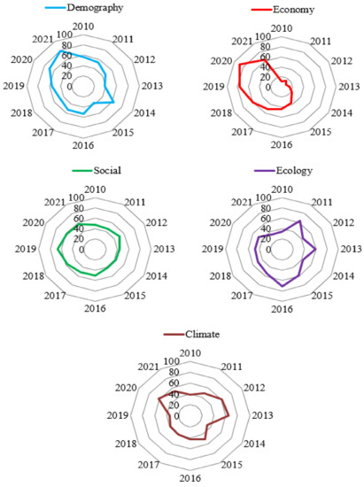
Figure 16.
Polygons for sustainable development of the Burabay district from 2010 to 2021.
The calculations made allow us to conclude that the sum of all indicators of SD of the Burabay district is developing positively (Figure 17). The development process has three distinct peaks in 2011, 2016 and 2020. However, in2021, the data went down sharply, which is most likely a result of COVID-19.
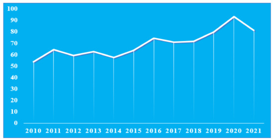
Figure 17.
Change in the sum of all indicators of the Burabay district over the past 12 years. (Ranking was carried out from 0 to 350, the minimum value for 2010 is 188, which is 53.71%).
Thus, the possibility of the integrated use of declarative or statistical information, spatial and temporal data, as well as demographic, economic, social, environmental, and climatic indicators for AD of an administrative-territorial region is shown.
4. Discussion
Despite the separate technical limitations described in the literature [53], when using the GEE platform, its positive aspects turned out to be much greater [54], which helped us quickly and with high accuracy perform the LULC classification of the Burabay district, where the city is located, NNP and AIC. To select the LULC classification method, before starting this process, we compared RF, CART and SVM. RF uses the construction of a big number of solutions and the application of balloting to the results. The primary example is used to recover the N tuition kits from the authentic dataset. Next, for each training sample, a decision tree (“forest”) is built. Every solution tree is autonomous and not referred to another [84]. CART is based on building a decision tree similar in principle to the RF method. Unlike RF, CART is a single decision tree and does not integrate a large number of decision trees [85]. SVM uses the construction of a classification rule using support vectors and has a lower classification accuracy near the boundary separating classes [86]. Therefore, we used RF as the main algorithm for classifying LULC from Landsat 7/8 images from 1991 to 2021. At the same time, we do not deny that in other studies, depending on the goals and objectives, the successful use of both CART and SVM is quite possible. The proof of this is the relatively small difference in overall accuracy between the algorithms used, equal to 0.93–097.
Next, the classification results based on RF were compared with the existing Land cover sets [74,75]. Our use of the Landsat series images (5/7/8) is dictated by the possibility of obtaining a long-time series of changes for AOI. For instance, the Land cover formed on the Sentinel 2 images covers the Burabay region only since 2015 [74]. Highly accurate and frequently repeated data from Planet [76] is still mostly commercial, but we also used their services [87] to refine the results of the LULC AOI classification. In addition, perhaps a significant role was played by our detailed acquaintance with this territory and its activities, as well as the availability of information from the land cadaster of Kazakhstan (https://aisgzk.kz/aisgzk/ru, accessed on 12 February 2023), which helped to make accurate training samples. At the same time, we are fully aware that, based on the presence of contrasting target objects (city, NPP, AIC), the unpredictability of the scenario for the development of events over more than 20 years and the difficulty in achieving absolute accuracy, such research areas as synthetic aperture could be useful radar (SAR) and hyperspectral images, which have significant potential to improve the methods of recognizing modification in land use [88].
The processes associated with the assessment of the achievement of the SDGs have led to an integrated approach to the study of land use, which includes partial or complete integration of socio-economic, environmental, and spatial temporal information [1,2]. This line of research, in turn, gave rise to many methodological approaches for assessing the defining criteria for the relationship between spatiotemporal data and economic, social and environmental information [40,89,90,91,92,93]. At the same time, in the context of our study, the use of relatively simple and understandable methods for a wide range of specialists turned out to be the most acceptable. These are RF—for LULC classification [94,95,96], multiple linear regression [97,98] and PCA—for determining the main driving forces [99,100,101], calculation of inter categorical transitions—for determining random and systematic changes [102,103] of classes LULLC and empirical calculation of sustainable development trend based on multi-stage transformations [1,88]. Perhaps the fact that we have limited ourselves to well-developed methods is a limitation of our work. But this assumption is justified by obtaining reliable results that helped to reach the purpose of the research.
The methodological procedures used clearly revealed the prime trend of land use change: a systematic growth in the space of CL, the same decrease in the share of pastoral, as well as random seizures of land from the forest cover for the construction of residential or other types of premises. Simultaneously, comparatively low growth in the city was noted, which stretched mainly in the other direction from the NNP and had almost no effect on the conservation and development of natural forests. Overall, our outcomes are in well convention with the general trends existing in the world as a whole [104,105] and in Kazakhstan in particular [106,107,108,109,110].
Spatiotemporal (LULC maps, NLT, precipitation, and temperature), as well as external statistical (economic, social, demographic, environmental) information, which made up 36 initial indicators, generally covered the entire range of SDGs. At the same time, it has been proven that the driving force behind the AOI is economic activity, including investment in the growth of the region. The leading role of the economy has been demonstrated in other studies of this kind [8,38]. In our opinion, the trend we identified is also of significant value, where a decrease in the rate of development of the integral indicator of the district under the influence of COVID-19 in 2021 was found. A similar trend under the influence of the pandemic was also found in many regions of the world [111,112].
In addition, the work performed is an organic continuation of our systematic research on the implementation of NSDI 2.0 and Land cover 2.0 in the activities of Kazakhstan [113], which is currently under implementation [114]. We believe that in the future, upon completion of the stages of creating an open system of coordinates and basic spatial data, when the phase of developing sectoral and thematic components, and strategic plans for the development of spatial data, the results of our research will become an important function of NSDI 2.0 of Kazakhstan. This is facilitated by the recently adopted “Law of the Republic of Kazakhstan on geodesy, cartography and spatial data” [115]. At present, our development is protected by copyright [116] and is still only part of one of the country’s geo services [117]. At the same time, future directions of research in other countries may be adjusted based on the level of development of space-time data and other circumstances: economic, environmental, social, political, as well as the level of technological development.
The studies carried out make a certain contribution to the evaluation of the development of the region, which has three relatively large functions aimed at improving the activities of agriculture, urban infrastructure, and the national natural park. The final results of the work can be used for subsequent planning of the territory and the development of an effective land use policy to achieve the SDGs.
5. Conclusions
The conducted studies have shown the effectiveness of assessing the development of an administrative-territorial district based on the integration of economic, environmental, and social indicators around spatiotemporal data. The proposed system of methodological approaches allowed: to process Landsat 5/7/8 space images using the high-performance web platform Google Earth Engine; to determine the dynamics of five Land Use and Land Cover classes from 1999 to 2021 based on the use of the machine learning method (RF algorithm) with high accuracy; to prove the steady increase in the composition of the Land Use and Land Cover Cropland classes and the decrease from year to year in the share of Pasture through the development and analysis of the Confusing and Transfer matrixes; to reveal that the main Driving Forces of Development of the Burabay district are economic factors, which was carried out using Multiple Regression Analysis and Principal Component Analysis; to show the Development trend of the Burabay district using multi-stage processing of 36 indicators combined into five groups (demographic, economic, environmental, social and climatic) from 2010 to 2021. It should be noted that the proposed set of methodological approaches is quite promising. For example, most of the leading experts in Kazakhstan still use only economic and statistical methods to assess sustainable development at the national level. For this, spatiotemporal data are not involved, the need for which has been convincingly proven by many works of researchers. The results of our study can be used to assess the sustainable development of the Burabay district based on the most objective instrumental spatiotemporal data, considering economic, social and environmental information. The developed system of methodological approaches can easily be scaled to analyze the development of larger administrative-territorial units.
Author Contributions
Conceptualization, O.A. and C.A.; methodology, O.A. and G.M.; validation, A.K., G.M. and P.G.; formal analysis, C.A.; investigation, G.M., P.G., M.A. and N.M.; resources, M.A.; data curation, N.M.; writing—original draft preparation, O.A. and G.M.; writing—review and editing, O.A. and C.A.; visualization, P.G.; supervision, O.A.; project administration, O.A.; funding acquisition, O.A. All authors have read and agreed to the published version of the manuscript.
Funding
This work was carried out within the framework of the program-targeted scientific and technical program “Research on the impact of state policy in the agricultural sector on the development of cooperative processes in the agro-industrial complex, sustainable development of rural areas and ensuring food security”, Individual Registration Number: BR 10764919, and has been funded by the Ministry of Agriculture of the Republic of Kazakhstan. Contract No. 17 from 9 January 2021.
Institutional Review Board Statement
Not applicable.
Informed Consent Statement
INot applicable.
Data Availability Statement
Not applicable.
Conflicts of Interest
The authors declare no conflict of interest.
Appendix A


Figure A1.
LULC maps of Burabay district from 1999 to 2021.
Figure A1.
LULC maps of Burabay district from 1999 to 2021.


Appendix B


Figure A2.
NLT maps of Burabay district from 1999 to 2021 (average for the year).
Figure A2.
NLT maps of Burabay district from 1999 to 2021 (average for the year).


Appendix C


Figure A3.
Precipitation maps of Burabay district from 1999 to 2021 (average for the month of May each year).
Figure A3.
Precipitation maps of Burabay district from 1999 to 2021 (average for the month of May each year).


Appendix D


Figure A4.
Temperature maps of Burabay district from 199 to 2021 (average for the month of June each year).
Figure A4.
Temperature maps of Burabay district from 199 to 2021 (average for the month of June each year).


References
- Sachs, J.; Lafortune, G.; Kroll, C.; Fuller, G.; Woelm, F. Sustainable Development Report 2022: From Crisis to Sustainable Development: The SDGs as Roadmap to 2030 and Beyond; Cambridge University Press: Cambridge, UK, 2022. [Google Scholar] [CrossRef]
- Oliveira, V.T.D.; Teixeira, D.; Rocchi, L.; Boggia, A. Geographic Information System Applied to Sustainability Assessments: Conceptual Structure and Research Trends. ISPRS Int. J. Geo Inf. 2022, 11, 569. [Google Scholar] [CrossRef]
- Turner, B.; Meyer, W.B.; Skole, D.L. Global land-use/land-cover change: Towards an integrated study. Ambio 1994, 23, 91–95. [Google Scholar]
- Parveen, S.; Basheer, J.; Praveen, B. A literature review on land use land cover changes. Int. J. Adv. Res. 2018, 6, 1–6. [Google Scholar] [CrossRef] [PubMed]
- GISGeography. Available online: https://gisgeography.com/free-global-land-cover-land-use-data/ (accessed on 5 February 2023).
- Planet. Available online: https://www.planet.com (accessed on 5 February 2023).
- Congalton, R.G.; Gu, J.; Yadav, K.; Thenkabail, P.; Ozdogan, M. Global Land Cover Mapping: A Review and Uncertainty Analysis. Remote Sens. 2014, 6, 12070–12093. [Google Scholar] [CrossRef]
- Hu, Y.; Hu, Y. Land Cover Changes and Their Driving Mechanisms in Central Asia from 2001 to 2017 Supported by Google Earth Engine. Remote Sens. 2019, 11, 554. [Google Scholar] [CrossRef]
- Ran, Y.; Li, X. First comprehensive fine-resolution global land cover map in the world from China—Comments on global land cover map at 30-m resolution. Sci. China Earth Sci. 2015, 58, 1677–1678. [Google Scholar] [CrossRef]
- Harsimran, K.; Garg, P. Urban Sustainability Assessment Tools: A Review. J. Clean. Prod. 2018, 210, 146–158. [Google Scholar] [CrossRef]
- Schneider, C.; Achilles, B.; Merbitz, H. Urbanity and Urbanization: An Interdisciplinary Review Combining Cultural and Physical Approaches. Land 2014, 3, 105–130. [Google Scholar] [CrossRef]
- Kanga, S.; Singh, S.K.; Meraj, G.; Kumar, A.; Parveen, R.; Kranjčić, N.; Đurin, B. Assessment of the Impact of Urbanization on Geoenvironmental Settings Using Geospatial Techniques: A Study of Panchkula District, Haryana. Geographies 2022, 2, 1–10. [Google Scholar] [CrossRef]
- Khor, N.; Arimah, B.; Otieno, R.O.; Oostrum, M.; Mutinda, M.; Martins, J.O. World Cities Report 2022: Envisaging the Future of Cities; UN-Habitat: Nairobi, Kenya, 2022. [Google Scholar]
- The World Bank. Available online: http://surl.li/esexa (accessed on 5 February 2023).
- Rozas-Vásquez, D.; Spyra, M.; Jorquera, F.; Molina, S.; Caló, N.C. Ecosystem Services Supply from Peri-Urban Landscapes and Their Contribution to the Sustainable Development Goals: A Global Perspective. Land 2022, 11, 2006. [Google Scholar] [CrossRef]
- Mitra, S.; Roy, S.; Hore, S. Assessment and forecasting of the urban dynamics through lulc based mixed model: Evidence from Agartala, India. GeoJournal 2022, 87, 1–24. [Google Scholar] [CrossRef]
- Cao, Y.; Huang, X.; Liu, X.; Cao, B. Spatio-Temporal Evolution Characteristics, Development Patterns, and Ecological Effects of “Production-Living-Ecological Space” at the City Level in China. Sustainability 2023, 15, 1672. [Google Scholar] [CrossRef]
- Combs, C.L.; Miller, S.D. A Review of the Far-Reaching Usage of Low-Light Nighttime Data. Remote Sens. 2023, 15, 623. [Google Scholar] [CrossRef]
- Mansour, S.; Ghoneim, E.; El-Kersh, A.; Said, S.; Abdelnaby, S. Spatiotemporal Monitoring of Urban Sprawl in a Coastal City Using GIS-Based Markov Chain and Artificial Neural Network (ANN). Remote Sens. 2023, 15, 601. [Google Scholar] [CrossRef]
- Xi, C.; Guo, Y.; He, R.; Mu, B.; Zhang, P.; Li, Y. The Use of Remote Sensing to Quantitatively Assess the Visual Effect of Urban Landscape—A Case Study of Zhengzhou, China. Remote Sens. 2022, 14, 203. [Google Scholar] [CrossRef]
- Gaur, S.; Singh, R. A Comprehensive Review on Land Use/Land Cover (LULC) Change Modeling for Urban Development: Current Status and Future Prospects. Sustainability 2023, 15, 903. [Google Scholar] [CrossRef]
- Waleed, M.; Sajjad, M.; Acheampong, A.O.; Alam, M.T. Towards Sustainable and Livable Cities: Leveraging Remote Sensing, Machine Learning, and Geo-Information Modelling to Explore and Predict Thermal Field Variance in Response to Urban Growth. Sustainability 2023, 15, 1416. [Google Scholar] [CrossRef]
- MDPI. Available online: https://www.mdpi.com/journal/urbansci (accessed on 5 February 2023).
- Yu, S.; Mu, Y. Sustainable Agricultural Development Assessment: A Comprehensive Review and Bibliometric Analysis. Sustainability 2022, 14, 11824. [Google Scholar] [CrossRef]
- Hu, S.; Yang, Y.; Zheng, H.; Mi, C.; Ma, T.; Shi, R. A framework for assessing sustainable agriculture and rural development: A case study of the Beijing-Tianjin-Hebei region, China. EIA Rev. 2022, 97, 106861. [Google Scholar] [CrossRef]
- Zanotti, L.; Ma, Z.; Johnson, J.L.; Johnson, D.R.; Yu, D.J.; Burnham, M.; Carothers, C. Sustainability, resilience, adaptation, and transformation: Tensions and plural approaches. Ecol. Soc. 2020, 25, 4. [Google Scholar] [CrossRef]
- Mallick, S.K. Prediction-Adaptation-Resilience (PAR) approach- A new pathway towards future resilience and sustainable development of urban landscape. Geogr. Sustain. 2021, 2, 127–133. [Google Scholar] [CrossRef]
- Mallick, S.K.; Das, P.; Maity, B.; Rudra, S.; Pramanik, M.; Pradhan, B.; Sahana, M. Understanding future urban growth, urban resilience and sustainable development of small cities using prediction-adaptation-resilience (PAR) approach. Sustain. Cities Soc. 2021, 74, 103196. [Google Scholar] [CrossRef]
- Mallick, S.K.; Rudra, S.; Maity, B. Unplanned urban built-up growth creates problem in human adaptability: Evidence from a growing up city in eastern Himalayan foothills. Appl. Geogr. 2023, 150, 102842. [Google Scholar] [CrossRef]
- Argaie, S.T.; Wang, K.; Lan, J. Urban land use efficiency in Ethiopia: An assessment of urban land use sustainability in Addis Ababa. Appl. Ecol. Environ. Res. 2022, 20, 3223–3244. [Google Scholar] [CrossRef]
- Dhawale, G.; Devne, M.; Ugale, V.; Ghosh, P.; Shirole, V.; Gosavi, P. Change Detection Analysis of Land Use Land Cover: A Case Study of Peri-Urban Area of Eastern Pune, M.S. Western India. Int. J. Early Child. Spec. Educ. 2022, 14, 276–295. [Google Scholar]
- Ittersum, M.K.; Ewert, F.; Heckelei, T.; Wery, J.; Olsson, J.A.; Andersen, E.; Bezlepkina, I.; Brouwer, F.; Donatelli, M.; Flichman, G.; et al. Integrated assessment of agricultural systems—A component-based framework for the European Union (SEAMLESS). Agric. Syst. 2008, 96, 150–165. [Google Scholar] [CrossRef]
- Sevilla, J.; Casanova-Salas, P.; Casas-Yrurzum, S.; Portalés, C. Multi-Purpose Ontology- Based Visualization of Spatio-Temporal Data: A Case Study on Silk Heritage. Appl. Sci. 2021, 11, 1636. [Google Scholar] [CrossRef]
- Assis, L.F.F.G.; Ferreira, K.R.; Vinhas, L.; Maurano, L.; Almeida, C.; Carvalho, A.; Rodrigues, J.; Maciel, A.; Camargo, C. TerraBrasilis: A Spatial Data Analytics Infrastructure for Large-Scale Thematic Mapping. ISPRS Int. J. Geo Inf. 2019, 8, 513. [Google Scholar] [CrossRef]
- Lambin, E.F. Linking Socioeconomic and Remote Sensing Data at the Community or at the Household Level. In People and the Environment, 1st ed.; Fox, J., Rindfuss, R.R., Walsh, S.J., Mishra, V., Eds.; Springer: New York, NY, USA, 2003; Volume 8, pp. 223–240. [Google Scholar]
- Cen, X.; Wu, C.; Xing, X.; Fang, M.; Garang, Z.; Wu, Y. Coupling Intensive Land Use and Landscape Ecological Security for Urban Sustainability: An Integrated Socioeconomic Data and Spatial Metrics Analysis in Hangzhou City. Sustainability 2015, 7, 1459–1482. [Google Scholar] [CrossRef]
- Hasan, S.; Shi, W.; Zhu, X.; Abbas, S. Monitoring of Land Use/Land Cover and Socioeconomic Changes in South China over the Last Three Decades Using Landsat and Nighttime Light Data. Remote Sens. 2019, 11, 1658. [Google Scholar] [CrossRef]
- Jiang, H.; Xu, X.; Guan, M.; Wang, L.; Huang, Y.; Liu, Y. Simulation of Spatiotemporal Land Use Changes for Integrated Model of Socioeconomic and Ecological Processes in China. Sustainability 2019, 11, 3627. [Google Scholar] [CrossRef]
- Naizhuo, Z.; Guofeng, C.; Wei, Z.; Eric, L.S.; Yong, C. Remote sensing and social sensing for socioeconomic systems: A comparison study between nighttime lights and location-based social media at the 500 m spatial resolution. Int. J. Appl. Earth Obs. Geoinf. 2020, 87, 102058. [Google Scholar] [CrossRef]
- Guo, X.; Ye, J.; Hu, Y. Analysis of Land Use Change and Driving Mechanisms in Vietnam during the Period 2000–2020. Remote Sens. 2022, 14, 1600. [Google Scholar] [CrossRef]
- Rudolf, J.; Udovč, A. Introducing the SWOT Scorecard Technique to Analyse Diversified AE Collective Schemes with a DEX Model. Sustainability 2022, 14, 785. [Google Scholar] [CrossRef]
- Barnosky, A.D.; Matzke, N.; Tomiya, S.; Wogan, G.O.U.; Swartz, B.; Quental, T.B.; Marshall, C.; McGuire, J.L.; Lindsey, E.L.; Maguire, K.C.; et al. Has the Earth’s Sixth Mass Extinction Already Arrived? Nature 2011, 471, 51–57. [Google Scholar] [CrossRef]
- On Approval of the List of Specially Protected Natural Areas of Republican Significance. Available online: https://adilet.zan.kz/rus/docs/P1700000593 (accessed on 5 February 2023).
- Koutika, L.-S.; Matondo, R.; Mabiala-Ngoma, A.; Tchichelle, V.S.; Toto, M.; Madzoumbou, J.-C.; Akana, J.A.; Gomat, H.Y.; Mankessi, F.; Mbou, A.T.; et al. Sustaining Forest Plantations for the United Nations’ 2030 Agenda for Sustainable Development. Sustainability 2022, 14, 14624. [Google Scholar] [CrossRef]
- Mabibibi, M.A.; Dube, K.; Thwala, K. Successes and Challenges in Sustainable Development Goals Localisation for Host Communities around Kruger National Park. Sustainability 2021, 13, 5341. [Google Scholar] [CrossRef]
- McCarthy, C.; Banfill, J.; Hoshino, B. National parks, protected areas and biodiversity conservation in North Korea: Opportunities for international collaboration. J. Asia Pac. Biodivers. 2021, 14, 290–298. [Google Scholar] [CrossRef]
- Job, H.; Bittlingmaier, S.; Mayer, M.; von Ruschkowski, E.; Woltering, M. Park–People Relationships: The Socioeconomic Monitoring of National Parks in Bavaria, Germany. Sustainability 2021, 13, 8984. [Google Scholar] [CrossRef]
- Christensen, M.; Jokar Arsanjani, J. Stimulating Implementation of Sustainable Development Goals and Conservation Action: Predicting Future Land Use/Cover Change in Virunga National Park, Congo. Sustainability 2020, 12, 1570. [Google Scholar] [CrossRef]
- Dimobe, K.; Gessner, U.; Ouédraogo, K.; Thiombiano, A. Trends and drivers of land use/cover change in W National park in Burkina Faso. Environ. Dev. 2022, 44, 100768. [Google Scholar] [CrossRef]
- UN-DESA (United Nations Department of Economic and Social Affairs). Transforming Our World: The 2030 Agenda for Sustainable Development; United Nations: Rome, Italy, 2015; p. 41. [Google Scholar]
- Liang, A.; Yan, D.; Yan, J.; Lu, Y.; Wang, X.; Wu, W. A Comprehensive Assessment of Sustainable Development of Urbanization in Hainan Island Using Remote Sensing Products and Statistical Data. Sustainability 2023, 15, 979. [Google Scholar] [CrossRef]
- Kalisz, B.; Żuk-Gołaszewska, K.; Radawiec, W.; Gołaszewski, J. Land Use Indicators in the Context of Land Use Efficiency. Sustainability 2023, 15, 1106. [Google Scholar] [CrossRef]
- Zhang, D.-D.; Zhang, L. Land Cover Change in the Central Region of the Lower Yangtze River Based on Landsat Imagery and the Google Earth Engine: A Case Study in Nanjing, China. Sensors 2020, 20, 2091. [Google Scholar] [CrossRef] [PubMed]
- Chen, D.; Wang, Y.; Shen, Z.; Liao, J.; Chen, J.; Sun, S. Long Time-Series Mapping and Change Detection of Coastal Zone Land Use Based on Google Earth Engine and Multi-Source Data Fusion. Remote Sens. 2022, 14, 1. [Google Scholar] [CrossRef]
- 716.kz. Available online: https://716.kz/raiony/23-burabaiskii-raion.html (accessed on 5 February 2023).
- adilet.zan.kz. Available online: http://gis-terra.kz/download/files/eno_shuchinsk_dendrarii_22_10_2018.pdf (accessed on 5 February 2023).
- Earth Engine Data Catalog. Available online: https://developers.google.com/earth-engine/datasets/catalog/LANDSAT_LE07_C02_T1_L2 (accessed on 5 February 2023).
- Earth Engine Data Catalog. Available online: https://developers.google.com/earth-engine/datasets/catalog/LANDSAT_LC08_C02_T1_TOA (accessed on 5 February 2023).
- Earth Engine Data Catalog. Available online: https://developers.google.com/earth-engine/datasets/catalog/NOAA_DMSP-OLS_NIGHTTIME_LIGHTS#description (accessed on 5 February 2023).
- Earth Engine Data Catalog. Available online: https://developers.google.com/earth-engine/datasets/catalog/NOAA_VIIRS_DNB_MONTHLY_V1_VCMCFG (accessed on 5 February 2023).
- Chander, G.; Markham, B.L.; Helder, D.L. Summary of current radiometric calibration coefficients for Landsat MSS, TM, ETM+, and EO-1 ALI sensors. Remote Sens. Environ. 2009, 113, 893–903. [Google Scholar] [CrossRef]
- Encyclopedia.com. Available online: https://www.encyclopedia.com/social-sciences-and-law/law/crime-and-law-enforcement/nima-national-imagery-and-mapping-agency (accessed on 5 February 2023).
- Colorado School of Mines. Available online: https://eogdata.mines.edu/products/dmsp/ (accessed on 5 February 2023).
- Colorado School of Mines. Available online: https://eogdata.mines.edu/products/vnl/ (accessed on 5 February 2023).
- Climatology Lab. Available online: https://www.climatologylab.org/terraclimate.html (accessed on 5 February 2023).
- Earth Engine Data Catalog. Available online: https://developers.google.com/earth-engine/datasets/catalog/MODIS_006_MCD43A4 (accessed on 5 February 2023).
- Google Earth Engine. Available online: https://earthengine.google.com/platform/ (accessed on 5 February 2023).
- Earth Engine Data Catalog. Available online: https://developers.google.com/earth-engine/datasets/catalog/LANDSAT_LC08_C01_T1_8DAY_EVI?hl=en (accessed on 5 February 2023).
- Earth Engine Data Catalog. Available online: https://developers.google.com/earth-engine/datasets/catalog/LANDSAT_LC08_C01_T1_8DAY_NDVI?hl=en (accessed on 5 February 2023).
- Earth Engine Data Catalog. Available online: https://developers.google.com/earth-engine/datasets/catalog/LANDSAT_LC08_C01_T1_8DAY_NDWI?hl=en (accessed on 5 February 2023).
- Earth Engine Data Catalog. Available online: https://developers.google.com/earth-engine/datasets/catalog/USGS_SRTMGL1_003 (accessed on 5 February 2023).
- Agency for Strategic Planning and Reforms of the Republic of Kazakhstan Bureau of National Statistics. Available online: https://stat.gov.kz/ (accessed on 5 February 2023).
- Statsnet. Available online: https://statsnet.co/companies/kz/55747 (accessed on 5 February 2023).
- Dynamic World. Available online: https://dynamicworld.app/ (accessed on 5 February 2023).
- Esa-WorldCover. Available online: https://esa-worldcover.org/en/data-access (accessed on 5 February 2023).
- Planet. Available online: https://www.planet.com/products/monitoring/ (accessed on 5 February 2023).
- ESA Global Land Cover System. Available online: https://viewer.esa-worldcover.org/worldcover/?language=en&bbox=71.26171627504557,51.171222211924345,71.34735110027266,51.192293461402045&overlay=false&bgLayer=MapBox_Satellite&date=2022-11-15&layer=WORLDCOVER_2021_MAP (accessed on 5 February 2023).
- Food and Agriculture Organization of the United Nations. Map Accuracy Assessment and Area Estimation: A Practical Guide; FAO: Rome, Italy, 2016; p. 69. [Google Scholar]
- Braimoh, A.K. Random and systematic land-cover transitions in northern Ghana. Agric. Ecosyst. Environ. 2006, 113, 254–263. [Google Scholar] [CrossRef]
- Pontius, R.G., Jr.; Shusas, E.; McEachern, M. Detecting important categorical land changes while accounting for persistence. Agric. Ecosyst. Environ. 2004, 101, 251–268. [Google Scholar] [CrossRef]
- Zewdie, W.; Csaplovics, E. Identifying Categorical Land Use Transition and Land Degradation in Northwestern Drylands of Ethiopia. Remote Sens. 2016, 8, 408. [Google Scholar] [CrossRef]
- A Step-by-Step Explanation of Principal Component Analysis (PCA). Available online: https://builtin.com/data-science/step-step-explanation-principal-component-analysis (accessed on 5 February 2023).
- Helwig, N.E. Multiple Linear Regression. Available online: http://users.stat.umn.edu/~helwig/notes/mlr-Notes.pdf (accessed on 5 February 2023).
- Matarira, D.; Mutanga, O.; Naidu, M. Google Earth Engine for Informal Settlement Mapping: A Random Forest Classification Using Spectral and Textural Information. Remote Sens. 2022, 14, 5130. [Google Scholar] [CrossRef]
- Wei-Yin, L. Fifty Years of Classification and Regression Trees. Int. Stat. Rev. 2014, 82, 329–348. [Google Scholar] [CrossRef]
- Support Vector Machines in Machine Learning (SVM): 2023 Guide. Available online: https://www.knowledgehut.com/blog/data-science/support-vector-machines-in-machine-learning (accessed on 5 February 2023).
- Planet. Order Schedule Number: Q03868 from October 31. 2021. Available online: https://www.planet.com/products/basemap/ (accessed on 5 February 2023).
- You, Y.; Cao, J.; Zhou, W. A Survey of Change Detection Methods Based on Remote Sensing Images for Multi-Source and Multi-Objective Scenarios. Remote Sens. 2020, 12, 2460. [Google Scholar] [CrossRef]
- Campagnolo, L.; Eboli, F.; Farnia, L.; Carraro, C. Supporting the UN SDGs transition: Methodology for sustainability assessment and current worldwide ranking. Economics 2018, 12, 20180010. [Google Scholar] [CrossRef]
- Angilella, S.; Catalfo, P.; Corrente, S.; Giarlotta, A.; Greco, S.; Rizzo, M. Robust sustainable development assessment with composite indices aggregating interacting dimensions: The hierarchical-SMAA-Choquet integral approach. Knowl. Based Syst. 2018, 158, 136–153. [Google Scholar] [CrossRef]
- Sharifi, A. Urban Resilience Assessment: Mapping Knowledge Structure and Trends. Sustainability 2020, 12, 5918. [Google Scholar] [CrossRef]
- Koppa, E.T.; Musonda, I.; Zulu, S.L. A Systematic Literature Review on Local Sustainability Assessment Processes for Infrastructure Development Projects in Africa. Sustainability 2023, 15, 1013. [Google Scholar] [CrossRef]
- Xu, Y.; Zhang, W.; Huo, T.; Streets, D.G.; Wang, C. Investigating the spatio-temporal influences of urbanization and other socioeconomic factors on city-level industrial NOx emissions: A case study in China. EIA Rev. 2023, 99, 106998. [Google Scholar] [CrossRef]
- Junaid, M.; Sun, J.; Iqbal, A.; Sohail, M.; Zafar, S.; Khan, A. Mapping LULC Dynamics and Its Potential Implication on Forest Cover in Malam Jabba Region with Landsat Time Series Imagery and Random Forest classification. Sustainability 2023, 15, 1858. [Google Scholar] [CrossRef]
- Garajeh, M.K.; Weng, Q.; Haghi, V.H.; Li, Z.; Garajeh, A.K.; Salmani, B. Learning-Based Methods for Detection and Monitoring of Shallow Flood-Affected Areas: Impact of Shallow-Flood Spreading on Vegetation Density. Can. J. Remote Sens. 2022, 48, 481–503. [Google Scholar] [CrossRef]
- Avcı, C.; Budak, M.; Yağmur, N.; Balçık, F. Comparison between random forest and support vector machine algorithms for LULC classification. IJEG 2023, 8, 1–10. [Google Scholar] [CrossRef]
- Yao, S.; Chen, C.; He, M.; Cui, Z.; Mo, K.; Pang, R.; Chen, Q. Land use as an important indicator for water quality prediction in a region under rapid urbanization. Ecol. Indic. 2023, 146, 109768. [Google Scholar] [CrossRef]
- Vardopoulos, I. Adaptive Reuse for Sustainable Development and Land Use: A Multivariate Linear Regression Analysis Estimating Key Determinants of Public Perceptions. Heritage 2023, 6, 809–828. [Google Scholar] [CrossRef]
- Forouhid, A.E.; Khosravi, S.; Mahmoudi, J. Noise Pollution Analysis Using Geographic Information System, Agglomerative Hierarchical Clustering and Principal Component Analysis in Urban Sustainability (Case Study: Tehran). Sustainability 2023, 15, 2112. [Google Scholar] [CrossRef]
- Islam, S.T.; Bhat, S.U.; Hamid, A.; Pandit, A.P.; Sabha, I. Impact of land-use patterns on water quality characteristics of Rambiarrah stream in Kashmir Himalaya. JRBM 2023. [Google Scholar] [CrossRef]
- Wang, X.; Yao, X.; Shao, H.; Bai, T.; Xu, Y.; Tian, G.; Fekete, A.; Kollányi, L. Land Use Quality Assessment and Exploration of the Driving Forces Based on Location: A Case Study in Luohe City, China. Land 2023, 12, 257. [Google Scholar] [CrossRef]
- Dan-Jumbo, N.G.; Metzger, M.J.; Clark, A.P. Urban Land-Use Dynamics in the Niger Delta: The Case of Greater Port Harcourt Watershed. Urban Sci. 2018, 2, 108. [Google Scholar] [CrossRef]
- Barnieh, B.A.; Jia, L.; Menenti, M.; Jiang, M.; Zhou, J.; Lv, Y.; Zeng, Y.; Bennour, A. Quantifying spatial reallocation of land use/land cover categories in West Africa. Ecol. Indic. 2022, 135, 108556. [Google Scholar] [CrossRef]
- Barati, A.A.; Zhoolideh, M.; Azadi, H.; Lee, J.-H.; Scheffran, J. Interactions of land-use cover and climate change at global level: How to mitigate the environmental risks and warming effects. Ecol. Indic. 2023, 146, 109829. [Google Scholar] [CrossRef]
- He, C.; Zhang, J.; Liu, Z. Characteristics and progress of land use/cover change research during 1990–2018. J. Geogr. Sci. 2022, 32, 537–559. [Google Scholar] [CrossRef]
- Qi, J.; Shiqi, T.S.; Pueppke, S.G.; Espolov, T.E.; Beksultanov, M.; Chen, X.; Cai, X. Changes in land use/land cover and net primary productivity in the transboundary Ili-Balkhash basin of Central Asia, 1995–2015. Environ. Res. Commun. 2020, 2, 011006. [Google Scholar] [CrossRef]
- Alipbeki, O.; Alipbekova, C.; Sterenharz, A.; Toleubekova, T.; Aliyev, M.; Mineyev, N.; Amangaliyev, K.A. Spatiotemporal Assessment of Land Use and Land Cover Changes in Peri-Urban Areas: A Case Study of Arshaly District, Kazakhstan. Sustainability 2020, 12, 1556. [Google Scholar] [CrossRef]
- Alipbeki, O.; Alipbekova, C.; Sterenharz, A.; Toleubekova, Z.; Makenova, S.; Aliyev, M.; Mineyev, N. Analysis of Land-Use Change in Shortandy District in Terms of Sustainable Development. Land 2020, 9, 147. [Google Scholar] [CrossRef]
- Samarkhanov, R.; Kozhokulov, J.S.; Chen, X.; Yang, D.; Issanova, G.; Aliyeva, S. Assessment of Tourism Impact on the Socio-Economic Spheres of the Issyk-Kul Region (Kyrgyzstan). Sustainability 2019, 11, 3886. [Google Scholar] [CrossRef]
- Samarkhanov, R.; Aliyeva, S.; Chen, X.; Yang, D.; Mazbayev, O.; Sekenuly, A.; Issanova, G.; Kozhokulov, S. The Socioeconomic Impact of Tourism in East Kazakhstan Region: Assessment Approach. Sustainability 2019, 11, 4805. [Google Scholar] [CrossRef]
- Nilashi, M.; Abumalloh, R.A.; Mohd, S.; Sharifah, N.F.S.A.; Sarminah, S.S.; Thi, H.H.; Alghamdi, O.A.; Alghamdi, A. COVID-19 and sustainable development goals: A bibliometric analysis and SWOT analysis in Malaysian context. Telemat. Inform. 2023, 76, 101923. [Google Scholar] [CrossRef]
- Nundy, S.; Ghosh, A.; Mesloub, A.; Albaqawy, G.A.; Alnaim, M.M. Impact of COVID-19 pandemic on socio-economic, energy-environment and transport sector globally and sustainable development goal (SDG). J. Clean. Prod. 2021, 312, 127705. [Google Scholar] [CrossRef]
- Alipbeki, O.A.; Alipbekova, C.A. Development of Spatial Data: Creation and Formation. S. Seifullin Kazakh Agrotechnical University: Nur-Sultan, Kazakhstan, 2020; p. 340. ISBN 978-601-257-284-1. (In Russian) [Google Scholar]
- adilet.zan.kz. Available online: https://adilet.zan.kz/rus/docs/V2000020535 (accessed on 5 February 2023).
- adilet.zan.kz. Available online: https://adilet.zan.kz/rus/docs/Z2200000166 (accessed on 5 February 2023).
- Alipbeki, O.A.; Alipbekova, C.A.; Mussaif, G.; Grossul, P.P.; Aliev, M.M.; Mineev, N.B. Algorithm for Determining the Driving Forces of the Development of the Administrative-Territorial District (Performed within the Framework of the Project BR10764919). The Republic of Kazakhstan. Certificate of Entering Information into the State Register of Rights to Objects Protected by Copyright No. 33631 Dated March 16, 2023. Available online: https://copyright.kazpatent.kz/?!.iD=wQEy (accessed on 5 March 2023).
- arcgis.gharysh.kz. Available online: https://arcgis.gharysh.kz/arcgis/apps/webappviewer/index.html?id=072892aed577460da804188ab4eb03d8 (accessed on 5 February 2023).
Disclaimer/Publisher’s Note: The statements, opinions and data contained in all publications are solely those of the individual |


Disclaimer/Publisher’s Note: The statements, opinions and data contained in all publications are solely those of the individual author(s) and contributor(s) and not of MDPI and/or the editor(s). MDPI and/or the editor(s) disclaim responsibility for any injury to people or property resulting from any ideas, methods, instructions or products referred to in the content. |
© 2023 by the authors. Licensee MDPI, Basel, Switzerland. This article is an open access article distributed under the terms and conditions of the Creative Commons Attribution (CC BY) license (https://creativecommons.org/licenses/by/4.0/).