Abstract
This paper introduces Split Delivery Clustered Vehicle Routing Problem with Soft cluster conflicts and Customer-related costs (SDCVRPSC) arising in automotive parts of milk-run logistics with supplier cluster distribution in China. In SDCVRPSC, customers are divided into different clusters that can be visited by multiple vehicles, but each vehicle can only visit each cluster once. Penalty costs are incurred when traveling between clusters. The transportation cost of a route is calculated as the maximum direct shipment cost between customers on the route plus the total drop costs. The SDCVRPSC aims to minimize the sum of transportation costs and penalty costs by determining the assignment of customers to vehicles and the visiting order of clusters. We propose an integer linear programming model and a two-level variable neighborhood descent algorithm (TLVND) that includes two-stage construction, intensification at cluster and customer levels, and a perturbation mechanism. Experimental results on designed SDCVRPSC benchmark instances demonstrate that TLVND outperforms the Gurobi solver and two adapted algorithms at the business operation level. Moreover, a real case study indicates that TLVND can bring significant economic savings compared to expert experience decisions. TLVND has been integrated into the decision support system of the case company for daily operations.
1. Introduction
Automotive manufacturers frequently utilize third-party logistics companies to complete parts pickup in a milk-run manner, allowing them to focus on the two high value-added links of product design and marketing [1]. In an automotive parts milk-run network, a logistics company develops efficient parts pick-up plans based on parts purchase orders of automotive manufacturers and corresponding parts supplier networks and arranges for several empty trucks to visit a few suppliers from the depot, collect a predetermined number of parts, and deliver them back to the depot to fulfill assembly line requirements. This process is often modeled as the classic Capacitated Vehicle Routing Problem (CVRP) [2,3,4,5,6,7,8,9]. With the increasing industrial concentration and scale of the automotive industry in China and worldwide, automotive parts suppliers are gradually clustering in industrial parks located in various cities, forming supplier clusters, which has a subtle impact on automotive parts logistics activities. CVRP under the clustering concept is typically known as Clustered VRPs, which include both cluster-level and customer-level route planning [10,11,12,13,14,15,16,17,18,19,20,21,22,23,24].
As the demand for automobiles in domestic and international (overseas) markets continues to rise, the production volume of automobile manufacturers and the business volume of logistics companies are also increasing. However, the application of Clustered VRPs in realistic milk-run business scenarios in China encounters operational limitations such as low resource utilization, high carbon dioxide emissions, and inflexible supplier visitation, which makes it impossible to realize an observable and controllable supply network [25,26,27,28]. In this paper, we conducted a field investigation into a third-party logistics company (TPL) that specializes in providing services to automotive manufacturers in China. Instead of directly executing the parts pickup plans, TPL focuses on logistics solution design and logistics network optimization and outsources the pickup process to carriers. This is because compared with owning their transportation capacity, this approach allows logistics companies to operate more flexibly and greatly reduces operational risks caused by industry fluctuations. To tackle the above challenges, for the outsourced plans, TPL only groups suppliers to specify which suppliers the carrier needs to visit and defines the visiting order of the clusters for each group without specifying the visiting order of the suppliers within the clusters. The carriers comprehensively consider the fuel consumption expenditure, traffic conditions, safety risks, and other factors, and combine their rich driving experience to retrieve the parts provided by suppliers to the depot according to the pickup plan. To calculate the salary paid to the carrier (TPL’s outsourcing cost), TPL adopts a new commercial contract which stipulates that the cost of each route includes the transportation cost and subsidy cost. The transportation cost of a route is equal to the maximum direct shipment cost between the suppliers on the route plus the total drop costs (if any), while the subsidy cost of the route is determined by the detour mileage of inter-cluster transportation. In Section 2.1, we provide a detailed description of all problem settings, realistic limitations, and corresponding business solutions.
Under this realistic contract, TPL is only required to group suppliers and specify the visiting order of clusters for each group of suppliers, without specific requirements for the visiting order of suppliers within each cluster. The objective of TPL is to efficiently allocate suppliers to vehicles and determine the optimal routes of vehicles at the cluster level to minimize the total transportation costs and subsidy costs. By regarding suppliers as customers, the cases where clusters can be visited by multiple vehicles as split delivery to clusters, the carrier’s preference for direct shipment to clusters as conflicts between clusters, and subsidy costs associated with inter-cluster transportation as penalty costs for violating the conflict relationship between clusters, we modeled the automotive parts milk-run problem with supplier cluster distribution as a Split Delivery Clustered Vehicle Routing Problem with Soft cluster conflicts and Customer-related costs (SDCVRPSC).
This paper analyzes the characteristics of the automatic parts milk-run problem with supplier cluster distribution from the perspective of TPL, proposes a new Clustered VRPs variant called SDCVRPSC, and designs effective heuristics to develop low-cost parts pickup plans. The proposed algorithm has been integrated into the decision support system of the case company to assist with operational management. The main contributions of this work are as follows. (1) Introducing a new and more realistic Clustered VRP, SDCVRPSC, which is derived from the automotive parts milk-run problem with supplier cluster distribution. (2) Providing an integer linear programming model for SDCVRPSC, and proposing the two-level variable neighborhood descent (TLVND) algorithm that combines two-stage construction, local search at the cluster and customer levels, and a perturbation mechanism. (3) Demonstrating that the proposed algorithm is expected to outperform two adapted heuristics and significantly reduce operational costs compared with the case company’s expert experience.
The remainder of this paper is structured as follows. Section 2 reviews the problems related to SDCVRPSC and emphasizes the similarities and differences with SDCVRPSC. Section 3 formally defines SDCVRPSC and presents the mathematical model. In Section 4, the proposed TLVND algorithm and two adapted heuristics are described in detail. Section 5 presents a comprehensive computational study on the designed benchmark cases and real cases. Section 6 concludes this paper and highlights future research directions.
2. Problem Setting and Literature Review
2.1. Problem Setting
The transportation problem under the concept of customer cluster distribution is usually modeled as Clustered VRPs, including two variants, Clustered VRP with hard-cluster constraints (CluVRP) [12,15,17,19,20,24,29], and Clustered VRP with soft-cluster constraints (SoftCluVRP) [16,21,23]. However, Clustered VRPs face the following limitations in real business applications.
Firstly, there is an uncertain size relationship between cluster demand and vehicle capacity. Clustered VRPs require that all customers within a cluster must be serviced by the same vehicle, provided that the total demand of all customers within a cluster respects the vehicle capacity. However, this premise is not feasible for parts pickup in automotive manufacturers. With the growth of the automotive industry and the rise in demand for parts, especially, such a condition is increasingly difficult to establish.
Secondly, split deliveries are both economically and practically necessary. When the remaining capacity of a vehicle is insufficient to meet the total demand of each remaining cluster, the split delivery strategy of serving specific customers in adjacent clusters along the way can effectively improve vehicle loading rates, reduce the number of dispatched vehicles, and minimize traveled distances [30,31]. Allowing split deliveries has been proven to be more conducive to reducing transportation costs by up to 50% [32].
Thirdly, there is a lack of driver experience and visiting flexibility. Clustered VRPs specify the visiting order of customers based on the shortest path, but uncontrollable factors such as traffic, weather, and accidents may render optimal routes impractical. In addition, experienced drivers usually plan better routes than optimization tools [27]. This is because drivers do not always follow the shortest path but rather consider road conditions (such as grocery stores and gas stations) and route simplicity (such as few traffic lights and turns).
Finally, maintaining the cost/distance matrix poses a significant challenge. Clustered VRPs aim to minimize total transportation cost/distance through a cost/distance matrix between all customers and the depot in the static traffic network. However, the matrix becomes very complex as the number of customers increases. It becomes a tough task to maintain the cost/distance matrix between all points and provide good route planning within an acceptable time for business.
The above limitations make Clustered VRPs impractical for the automotive parts milk-run problem and lead to gaps in practice and research. In this paper, we investigate the case company, TPL, whose business model effectively addresses the gaps. TPL provides a part-picking plan by grouping customers and only specifying the visiting order of the clusters for each group, because intra-cluster transportation is more susceptible to uncontrollable factors and requires route adjustment compared to stable long-distance inter-cluster transportation on highways. The carriers, as the outsourcers of TPL, can decide their visiting order of customers within each cluster based on extensive driving experience to avoid the impact of these uncontrollable factors. However, the unknown nature of the carriers’ actual visit routes makes the traditional cost calculation manner based on traveled distance inapplicable. Therefore, TPL specially signs a new business contract with the carriers to calculate the outsourcing cost, i.e., the salary paid to the carriers, to avoid the impact of customer visiting sequence.
This business model has several key features. First, the transportation cost of a route is calculated as the maximum direct shipment cost from the depot to all customers on the route plus the drop cost of other customers on the route except one with the maximum direct shipment cost (if any), which is also applied to the metal packaging industry [33]. This approach simplifies the cost calculation by reducing the cost/distance matrix to a one-dimensional vector. Second, compared to short-distance intra-cluster transportation, long-distance inter-cluster transportation brings higher expenditure to the carrier (e.g., fuel consumption, safety risks caused by fatigue driving, etc.). When clusters are in opposite geographical directions on the route, the carrier’s actual expenditure will be much higher than the salary paid by TPL, as the direct shipment of a single cluster or even a single customer can yield higher revenues. Therefore, TPL pays additional subsidies based on the detour mileage of inter-cluster transportation to promote consolidated transportation. Third, the goal of TPL is to minimize the outsourcing cost, which includes transportation costs and subsidy costs.
Based on the above practical background analysis, the characteristics of the proposed SDCVRPSC problem are summarized as follows:
- Cluster-level route planning. In CVRP, the visiting order of each group of customers is usually further specified after grouping customers. However, in the case of customer cluster distribution, only the visiting order of the cluster corresponding to each group of customers is specified, and the visiting order of customers within each cluster can be decided by the driver experience.
- Split delivery at the cluster level. Since the size relationship between cluster demand and vehicle capacity is uncertain, the cluster demand can be split among multiple vehicles. Therefore, a vehicle does not need to visit all customers within a cluster without exceeding the capacity limit. As considered in the Split Delivery Vehicle Routing Problem (SDVRP, see Archetti et al. [34]), this allows a customer to be visited by multiple vehicles, resulting in significant savings in the total distance traveled and the number of vehicles used.
- Soft cluster conflicts. The long transportation distances between clusters are much greater than the distances between customers within the cluster. The carrier’s preference for the direct shipment of a single cluster rather than consolidated transportation between clusters can be regarded as a conflict between clusters. In this scenario, the subsidy costs associated with inter-cluster transportation act as penalty costs for violating the conflict relationship between clusters.
- Customer-related costs. The cost-calculating model avoids the impact of the order of customer visits on the transportation cost, making the cost of each vehicle dependent on the direct shipment costs and quantities of the customers visited. Additionally, penalty costs are further related to the clusters corresponding to the customers visited.
2.2. Literature Review
SDCVRPSC can be seen as a new variant of Clustered VRPs. As mentioned earlier, there are two main variants of VRPs under the concept of customer cluster distribution: CluVRP and SoftCluVRP. In Table 1, we provide a non-exhaustive overview of research on Clustered VRPs and classify them according to the proposed solutions (exact vs. heuristic algorithms). Because of the NP-hard nature of the problem, most of the literature on Clustered VRPs focuses on heuristics.

Table 1.
Literature on (Soft)CluVRPs, while Heu/Ex specifies if the problem is solved heuristically (Heu) or exactly (Ex) by the corresponding solution approach(es).
CluVRP was introduced by Sevaux and Sörensen [35] to model a real-world parcel delivery problem in courier companies where customers are pre-segmented into different clusters and all customers belonging to the same cluster must be visited continuously by the same vehicle. The following exact approaches are proposed to address CluVRP. Pop et al. [11] described CluVRP as an extension of the Generalized Vehicle Routing Problem (GVRP, Ghiani and Improta [36]) and adapted two compact formulations of GVRP to CluVRP by adding additional constraints. In another study based on the integer programming formulation, Battarra et al. [12] proposed two exact solution approaches where the branch-and-cut based on the pre-calculated intra-cluster paths was superior to the branch-and-cut-and-price.
Several heuristics have been developed for CluVRP. Barthélemy et al. [10] added an extremely large value to all inter-cluster edges to convert CluVRP into CVRP and solve it by simulated annealing. Vidal et al. [14] proposed two hybrid metaheuristics, iterative local search and unified hybrid genetic search, to solve CluVRP, but obtained high-quality solutions at the expense of very high calculation times. Expósito-Izquierdo et al. [15] divided CluVRP into two subproblems: a high-level routing problem determining routes targeted at visiting the clusters (inter-cluster), and a low-level routing problem finding a visiting order of the customers belonging to each cluster (intra-cluster). The record-to-record travel algorithm and three different technologies were used to solve the low-level routing problem: the mixed integer linear programming model, the exact solution based upon decision-tree search, and the Lin–Kernighan–Helsgaun heuristic (LKH, see Lin and Kernighan [37] and Helsgaun [38]) were used to solve these two subproblems, respectively. Defryn and Sorensen [16] suggested a fast two-level variable neighborhood search (Two-level VNS) to solve both level routing problems of CluVRP. Horvat-Marc et al. [18] presented a genetic algorithm to solve the high-level routing problem and a simulated annealing approach to solve the low-level routing problem. A similar approach was proposed by Pop et al. [19], in which the cluster-level routing problem was also solved with a genetic algorithm, while the customer-level was transformed into the well-known traveling salesman problem (TSP) by the Concorde TSP solver. Hintsch and Irnich [17] decomposed CluVRP into three subproblems: cluster assignment problem, inter-cluster routing problem, and intra-cluster routing problem, and proposed a large multiple neighborhood search (LMNS) based on multiple destroy and repair operators and a variable neighborhood descent for post-optimization. Xu et al. [20] presented the shortest distance best fit decreasing algorithm to construct the initial solution, and adapted variable neighborhood search and Lin–Kernighan considering virtual points to improve inter-cluster and intra-cluster routing. Aerts et al. [22] modeled the joint order batching and picker routing problem as CluVRP, and proposed an adapted version of the Two-level VNS presented by Defryn and Sorensen [16]. Islam et al. [24] proposed a hybrid metaheuristic, combining the particle swarm optimization (PSO) and VNS, and proved that the proposed algorithm was superior to the state-of-the-art algorithms on CluVRP.
The first study of SoftCluVRP was conducted by Defryn and Sorensen [16], who referred to it as the CluVRP with weak cluster constraints. They acknowledged that the travel distance could be reduced if vehicles were allowed to leave the cluster to serve another cluster first (partially), and then return to the initial cluster afterwards to visit the remaining customers, and solved it by slightly adapting their Two-level VNS for CluVRP. Hintsch and Irnich [21] formally defined the CluVRP with weak cluster constraints as SoftCluVRP, designed different branch-and-price algorithms for the exact solution of SoftCluVRP, and confirmed that relaxing cluster constraints can reduce the total travel distance by 6.21% on average. Later, Hintsch [23] made major modifications to LMNS developed for CluVRP [17] to solve SoftCluVRP and provided new best-known solutions for more than half of the medium-sized instances.
The SDCVRPSC proposed in this paper differs from the above two Clustered VRPs. In terms of the problem setting, it is different from CluVRP in that (1) SDCVRPSC does not limit the relationship between the cluster demand and vehicle capacity, and split delivery at the cluster level exists, allowing multiple vehicles to enter and leave the same cluster. (2) Once a vehicle enters a cluster, it must visit all customers in the assigned subcluster of that cluster continuously, not necessarily the entire cluster. (3) Penalty costs incur when vehicles move from one cluster to another, which leads to the soft conflict relationship between clusters. (4) SDCVRPSC considers the flexibility of customer visits, does not specify a specific order of customer visits after the vehicle enters a cluster, and customer-related costs bring new cost structure and optimization objectives. Compared with SoftCluVRP, except for the four differences mentioned above, SDCVRPSC does not allow vehicles to leave and re-enter a cluster multiple times during its trip.
3. Problem Statement and Model Formulation
3.1. Problem Statement
The sets, parameters, and variables for the problem description and mathematical formulation of SDCVRPSC are defined in Table 2.
Table 2.
List of notations.
The SDCVRPSC is defined as follows: given an undirected graph , the set represents all customer clusters, where cluster 0 includes only the depot, and all other clusters contain at least one customer. Each cluster is represented by a cluster center, and different bypass miles exist based on the geographical locations of different clusters, corresponding to a certain penalty cost. The edge is associated with a penalty cost for transportation between cluster and cluster , representing the conflict relationship between different clusters. Unlike the common practice in the existing literature of assigning 0 or 1 for conflicts, this paper uses different levels of penalty costs to reflect the fact that not all conflicts should incur the same level of penalty in practice.
Suppose there is a set of customers to be visited, where 0 represents the depot, and the demand, direct shipment cost, and cluster of each customer are , , and . The available vehicle fleet is homogeneous, and the maximum vehicle capacity is . Each vehicle starts from the depot, visits some customers, and returns to the depot without violating the vehicle capacity limit, requiring each customer to be visited only once. For each vehicle , the transportation cost is equal to the maximum direct shipment cost plus drop cost , and the penalty cost is determined by the visiting order among the clusters.
Without losing generality, we assume that each customer demand and vehicle capacity meet , and each cluster demand and vehicle capacity meet or . Define the subset as the set of customers in cluster . SDCVRPSC aims to minimize the sum of transportation costs and penalty costs by determining the optimal allocation of customers to vehicles and specifing the visiting order of the cluster.
3.2. Model Formulation
The SDCVRPSC can be formulated as the following integer linear programming model:
In this model, the objective function (1) minimizes the overall cost of all vehicles, including transportation costs and penalty costs. Constraint (2) requires that each customer is visited exactly once. Constraint (3) ensures the vehicle capacity is not exceeded. Constraint (4) assures that the number of vehicles used does not exceed the number of available vehicles. Constraints (5)–(8) calculate the maximum direct shipment cost, drop cost, transportation cost, and penalty cost of each vehicle, respectively. Constraint (9) ensures that the same vehicle can only arrive at and leave a given cluster once. Constraint (10) states that clusters can be visited by multiple vehicles. Constraint (11) represents the subtour elimination. Constraints (12) and (13) are used to associate the decision variables in constraint (15), indicating that a customer is visited by a vehicle on the premise that the vehicle is used and visits the cluster to which the customer belongs. Constraint (14) reduces the problem’s solution space by ensuring unused bins have higher indexes than used ones. Constraint (15) restricts the variables to be binary.
When all suppliers belong to a single cluster, resulting in no penalty cost for inter-cluster transportation, this problem can be viewed as the bin packing problem (BPP), where customers are treated as items and vehicles as bins. When each cluster only has one supplier, there is no intra-cluster routing, making it equivalent to CVRP. Since BPP and CVRP are both well-known to be NP-hard, SDCVRPSC is also NP-hard.
3.3. Numerical Example
To better illustrate the problem, an example of SDCVRPSC is given below, as shown in Figure 1. Sixteen customers numbered 1–16 are distributed in Clusters A–F. The red square represents the depot, the circles represent the customers, and the customers in the same dotted box belong to the same cluster. The demand and direct shipment cost of customer are represented by the coordinate . Assume that the maximum vehicle capacity is 10, and the drop cost per visit is 2. The penalty costs between the six clusters are pre-defined by the conflict matrix in Table 3. Since the long-distance distance between clusters is much larger than the last-mile logistics activity distance within each cluster, the distance between clusters and the distance between customers within clusters are scaled in a certain proportion for the visualization and intuitionism of transportation routes.
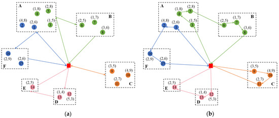
Figure 1.
An illustrative example of SDCVRPSC. (a) A feasible transportation scheme (without intra-cluster routes) of TPL; (b) a feasible transportation scheme (with intra-cluster routes) of carriers.
Table 3.
Penalty costs between clusters.
A feasible transportation scheme developed by the TPL for the carrier consists of supplier grouping and inter-cluster routes, as shown in Figure 1a. Each color represents a route; that is, customers with the same color are visited by the same vehicle. In Route 1 (blue), the vehicle starts from the depot, first enters Cluster A to visit customers 1 and 2, then enters Cluster F to visit customers 15 and 16, and finally returns to the depot. The maximum direct shipment cost of Route 1 is 9 (the cost of customer 16), and the drop cost for three additional visits to customers 1, 2, and 15 is 6, so the transportation cost of Route 1 is 15. In addition, Route 1 carries out inter-cluster transportation from Cluster A to Cluster F, which incurs a penalty cost of 7. Therefore, the total cost of Route 1 is the sum of transportation cost and penalty cost, i.e., 22. Similarly, Route 2 (green) has a total cost of 27, Route 3 (orange) has a total cost of 13, and Route 4 (pink) has a total cost of 14. Therefore, the overall cost required to complete the visits of 16 customers is the sum of the costs of the four routes, i.e., 76. At the same time, based on the route planning of TPL, the carrier can comprehensively consider the fuel consumption expenditure, traffic conditions, safety risks, and other factors (as mentioned in Section 2.1) and combine rich driving experience to decide the visiting order of customers in each cluster (intra-cluster routes), pursuing a low-cost and low-risk route. A feasible transportation scheme for the carrier is shown in Figure 1b. For the above four routes, carriers enter each cluster according to the specified inter-cluster routes, and determine the intra-cluster routes based on multiple factors; that is, they enter the corresponding cluster and visit the corresponding suppliers in the sequence of arrows.
4. Solution Methodology
SDCVRPSC arises naturally from the real-world automotive parts milk-run problem with supplier cluster distribution, and its business operation is highly time-sensitive, so it needs to generate a transportation scheme quickly. However, solving large-scale problems can be time-consuming since SDCVRPSC is NP-hard; hence, it is crucial to explore heuristics that can provide TPL with immediate decision support by generating approximately optimal or satisfactory solutions within an acceptable time.
4.1. Overview
The solution process for CVRP and its variants always follows a common two-stage strategy, consisting of a route construction phase and a subsequent local search phase. Referring to Defryn and Sorensen [16], this paper proposes the Two-level Variable Neighborhood Descent (TLVND) algorithm, which consists of three phases: (a) construction; (b) intensification; and (c) diversification. The overall framework of TLVND is shown in Algorithm 1. The construction phase uses a two-stage heuristic to generate the initial solution. The intensification phase explores the solution space by VND at both the cluster and supplier levels, where neighborhood operators are designed based on the problem characteristics to find a local optimum. To facilitate the search process, the solution obtained at the cluster level is used as the input for the customer-level VND. During the diversification phase, a permutation operator perturbs the solutions that have been optimized at both levels, and the algorithm enters the local search phase again. The maximum number of iterations in the algorithm is set to , and it terminates when no further improvement is observed after consecutive iterations.
| Algorithm 1 Outline of Two-level Variable Neighborhood Descent |
| Input: Output: 1: 2: 3: 4: ▷Construction 5: While do ▷Intensification 6: VND- 7: 8: While do 9: 10: if then 11: 12: 13: else 14: 15: if then 16: 17: break 18: end if 19: end if 20: ) ▷Diversification 21: random number in [0, 1] 22: if then 23: 24: else 25: 26: end if 27: end while 28: 29: if then 30: 31: break 32: end if 33: end while |
4.2. Construction Phase
In the construction phase, the primary task is to obtain a feasible solution for SDCVRPSC, rather than the optimal solution. Hence, a fast algorithm that generates a feasible initial solution is preferable [16]. The SDCVRPSC can be tackled by establishing cluster visit routes after assigning customers to vehicles, which decomposes the problem into two subproblems: the customer assignment problem (CAP), which involves grouping customers to obtain an assignment scheme between customers and vehicles, and the cluster sequence problem (CSP), which focuses on determining the order of visits to the clusters for each customer group. The solution obtained by a decomposition method is not as good as the one found by solving the whole problem, but this limitation can be overcome by using an iterative solution process and in this way improving iteratively the solution of the subproblems [15,19].
To obtain a feasible solution, we propose a two-stage heuristic (Algorithm 2) to solve the two successive subproblems. The first stage employs the best fit decreasing with cluster and cost (BFDCC) to tackle the CAP, while the second stage uses the LKH to solve the CSP. The initial solution for SDCVRPSC can be directly obtained by combining the solutions of the two subproblems without using any post-processing procedures. Further details are given in subsequent chapters.
| Algorithm 2 Two-stage Heuristic |
| Input: Output: 1: ▷First-stage 2: Solve the CAP instance by BFDCC 3: 4: for ) do ▷Second-stage 5: 6: and a virtual point 7: Solve the CSP instance by LKH 8: Solution 9: end 10: ▷Combination |
4.2.1. Customer Assignment Problem
In the first stage, CAP needs to be solved by partitioning customers into vehicles to obtain the corresponding transportation costs. CAP can be modeled as a BPP where a set of items (customers) with a given weight (demand) will be packed into a set of bins (vehicles) with the maximum capacity. One of the most commonly used algorithms in the literature, best fit decreasing (BFD, see Johnson [39]), packs each item in descending order of weight into the fullest bin consecutively. This is satisfactory for a simple packing problem, but when solving the Clustered VRPs it is important that clusters assigned to the same vehicle can be used later to construct efficient routes.
By analyzing the characteristics and objectives of SDCVRPSC, to minimize transportation costs and penalty costs per vehicle, firstly, customers with close direct shipment costs should be visited together as much as possible, because all customers except one with the maximum direct shipment cost pay a much smaller drop cost rather than their full direct shipment cost. Secondly, visiting customers in the same cluster together as much as possible can reduce the number of split deliveries at the cluster level and inter-cluster transportation. Finally, customers in adjacent clusters should be arranged in one vehicle as much as possible, which avoids customers in different directions being placed in one vehicle to incur higher penalty costs.
In this paper, we adopted best fit decreasing with cluster and cost (BFDCC) to complete customer assignment. Specifically, we sorted all clusters in descending order by the average direct shipment cost of all customers in the cluster, and then by the number of customers in the cluster. Then, we sorted all customers in each cluster in descending order by the direct shipment cost and then by demand. Finally, with the premise of sufficient remaining capacity of the vehicle, we arranged each sorted customer in turn by the vehicle that had visited the cluster nearest to the customer cluster (including the cluster where the customer belongs). If multiple vehicles had visited the cluster closest to the customer’s cluster, the vehicle with the minimum remaining capacity is selected.
4.2.2. Cluster Sequence Problem
In the second stage, the clusters corresponding to each customer and assigned to each vehicle are first counted in the customer grouping scheme obtained in the first stage. Then, the visiting order of clusters for each vehicle is determined to obtain the penalty cost for inter-cluster transportation from the first visited cluster to the last one. This problem can be formulated as the Shortest Hamiltonian Path Problem (SHPP, see Christofides [40]) when minimizing the travel costs, which is expressed as follows: in the undirected graph consisting of cluster visited by vehicle , the weight of edge is considered as the penalty cost for a vehicle to travel from cluster to cluster , and the goal is to find the shortest path where each cluster is visited only once.
To determine the order of cluster visits for each vehicle, we converted the corresponding SHPP to TSP by adding a virtual point; specifically, the travel cost from the virtual point to each cluster was set to 0, the travel cost between each cluster was defined as the penalty cost corresponding to inter-cluster transportation, and the travel cost from each cluster to itself was set to an extremely large to avoid the situation where a vehicle departs from a cluster and returns to that cluster. Since LKH is widely recognized as one of the most effective techniques to solve TSP, we adopted it as an indirect means to solve CSP.
4.3. Intensification Phase
The two-stage heuristic provides a feasible solution for SDCVRPSC. However, the local optimality of the solution is not guaranteed. The intensification phase aims to explore the search space to find solutions with lower objective values until a local optimum is reached. Considering the customer cluster distribution characteristics and the cost calculation model, this paper performed a two-level optimization of the initial solution, at the cluster level and customer level, and both levels used VND to find the local optimal solution based on the corresponding neighborhood operators.
As for the analysis of SDCVRPSC characteristics in Section 4.2.1, to minimize the transportation cost and penalty cost per vehicle, the customers in adjacent clusters are expected to be arranged on a route as much as possible to improve the chance of consolidated transportation to mainly reduce penalty costs, while the customers with similar transportation cost are visited together as much as possible to mainly reduce transportation costs. Therefore, we first performed a local search on the cluster level to optimize the cluster distribution of vehicles, and then performed a local search on the customer level to optimize the customer distribution with the optimized cluster vehicle assignment.
Furthermore, customer-related costs ensure that the intra-route neighborhood operations do not change the customers visited by each vehicle, nor do they change the optimal visiting order of each vehicle among the corresponding clusters, thus not changing the total cost of the route, so this paper explores the inter-route neighborhoods by adapting the well-known neighborhood operators relocate, swap, and swap2vs1 for different routes.
4.3.1. Intensification at the Cluster Level
At the first level of the intensification phase, a local search with the cluster as the minimum granularity of the initial solution was performed to find the optimal cluster visiting list and order for each vehicle. The split delivery at the cluster level allowed some clusters to be visited by multiple vehicles, forming multiple subclusters. We called these split clusters the parent clusters of these subclusters. Cluster-level optimization requires that customers belonging to a subcluster will be visited as a whole, which limits the number of feasible moves to be checked by neighborhood operators.
This paper provides inter-route operators, as shown in Table 4. During the three neighborhood searches, if two or more subclusters belonging to the same parent cluster appear on the same route, the visiting order of the subclusters on that route is determined by the visiting order of that parent cluster to ensure that each vehicle visits each cluster only once. By operating subclusters on different routes, inter-route operators change the clusters visited by vehicles while bringing changes in the corresponding visited customers. Therefore, intensification at the cluster level aims to optimize the vehicle capacity distribution to increase vehicle loading rates and optimize the cluster distribution of vehicles to facilitate consolidated transportation, thus reducing the transportation costs and penalty costs of the vehicles, and ultimately improving the overall cost of the solution.
Table 4.
Different neighborhoods at the cluster level.
For each operator, we only considered all feasible moves that led to objective improvement under the capacity constraint, which could reduce the size of the explored neighborhood. Due to the high computational cost of recalculating the objective function after each move, we only calculated the objective increment for the two routes involved in each move. The cluster-level VND executes each inter-route operator sequentially and adopts the first move strategy for all local search moves. The algorithm moves to the next neighborhood if the solution has not received any improvement in the current one and restarts by exploring the first neighborhood once the improvement is found. It repeats until no neighborhood can further improve the current solution, and reaches a local optimal at the cluster level.
4.3.2. Intensification at the Customer Level
The second level in the intensification phase is a local search with customers as the minimum unit for the solution reinforced by VND at the cluster level, aimed at finding the optimal customer assignment for each vehicle. It must be considered that moving a customer in a cluster of the current route to another target route that has not yet visited the customer’s cluster will not increase the penalty cost of the current route but will increase the penalty cost of the target route, resulting in an increase in the global penalty cost. Therefore, this paper provides customer-level inter-route operators (see Table 5), which require that the target route of a customer must pass through its cluster and the customer is assigned to the corresponding subcluster so that the algorithm enters a more promising search space. Since clusters are allowed to be split, the existence of subclusters makes swap and swap2vs1 operators include both inter-cluster and intra-cluster moves, acting on two customers in the same cluster and different clusters on different routes, respectively. Therefore, intensification at the customer level optimizes the customer distribution of vehicles to improve vehicle full load rates, and reduces the global transportation cost without disturbing the cluster visiting order of the vehicles determined by the intensification at the cluster level; i.e., the clusters are visited in the most efficient sequence possible.
Table 5.
Different neighborhoods at the customer level.
Like the intensification at the cluster level, we adopted the first move strategy for VND at the customer level and only calculated the objective increment of the two related routes to obtain a local optimum.
It is worth mentioning that since the intensification phase is the most time-critical part for the proposed TLVND, we introduced the “time stamps” in the VND at both the cluster and the customer levels and recorded the moves that had been evaluated but not improved by registering “last modification time of the route” and “last evaluation time of the moves associated to a given customer”, thereby avoiding duplicate searches and significantly speeding up the local search [41].
4.4. Diversification Phase
In the diversification phase, the algorithm explores the previously unexplored region of the search space. The algorithm moves from the customer level to the cluster level using a perturbation mechanism, which successively removes and inserts entire subclusters instead of individual customers through the destroy operator and repair operator, where the parameter indicates the percentage of subclusters that needs to be removed. The destroy operator randomly selects subclusters to remove from the position of the current route. The repair operator is responsible for reinserting each removed subcluster randomly to a position in another route. To guarantee that the vehicle capacity constraint is not violated, only feasible insertions are considered, i.e., the demand of the inserted subclusters does not exceed the remaining capacity of the vehicle.
After obtaining a new solution in the diversification phase, the algorithm can restore its local search at the cluster level or at the customer level. Referring to Defryn and Sorensen [16], this process is controlled by the parameter . A random probability is generated, and if , the new solution is first improved via the intensification phase at the cluster level followed by the intensification phase at the customer level, otherwise the algorithm directly calls the optimization at the customer level.
4.5. Adapted Heuristics
For subsequent experiments to verify the performance of TLVND, this paper modified the classical FFD and the effective solution algorithm for CluVRP to solve the SDCVRPSC problem.
4.5.1. First Fit Decreasing in Demand and Cost with LKH
As analyzed in Section 4.2.1, to minimize the overall cost of transportation and penalty costs, this paper proposes the first fit decreasing in demand and cost with LKH (FFDDC_LKH) based on FFD to minimize the number of split deliveries to clusters, i.e., customers in the same cluster are visited by the same vehicle as much as possible, and subsequently aims for customers with similar direct shipment costs in the same cluster to be scheduled on a route as far as possible. The details are as follows.
- Step 1:
- Calculate the total demand of each cluster, i.e., the sum of the demand of all customers in the cluster.
- Step 2:
- Sort the clusters in descending order according to the total demand, and then sort all customers in each cluster first according to the direct shipment cost and then the demand in descending order.
- Step 3:
- Assign each sorted customer in turn to the first vehicle with sufficient remaining capacity.
- Step 4:
- For each vehicle, the LKH is used to determine the visiting order of clusters.
4.5.2. Adapted CluVRP Solution Approach
In SDCVRPSC, the cluster demand may not necessarily be (much) smaller than the vehicle capacity, thus requiring split delivery at the cluster level. Section 4.2.1’s analysis highlights the need to minimize the number of cluster splitting visits to reduce transportation costs and penalty costs, so we converted SDCVRPSC instances into CluVRP instances by pre-splitting cluster with the total customer demand exceeding vehicle capacity into as few subclusters as possible, and set the penalty cost among these subclusters to 0. This split operation can be viewed as BPP, i.e., customers with demands are viewed as items with weights, vehicle capacity is viewed as bin capacity, and minimizing the number of cluster splitting visits is minimizing the number of bins used. Then, the split operation of cluster can be carried out by FFD and the lower bound of the number of splits is .
To address the SDCVRPSC instances transformed into CluVRP problems, this paper adopts the excellent two-level VNS algorithm proposed by Defryn and Sorensen [16] for solving CluVRP. In contrast to the two-level subproblems of CluVRP (inter-cluster routing problem and intra-cluster routing problem), SDCVRPSC does not specify the visiting order of customers within a cluster. Therefore, considering the problem characteristics, we discarded the intra-cluster path construction and local search at the customer level in Two-level VNS. Instead, we planned the routes for the subclusters to obtain the initial solution for SDCVRPSC. Therefore, the adapted Two-level VNS was as follows. Firstly, the inter-cluster routing plan was achieved by BFD: sort each subcluster first by the demand of its parent cluster, and then by its demand in descending order; assign each sorted subcluster to the first bin where the nearest subcluster (including the cluster it belongs to) is located if the capacity allows; and regard the packing order of the subcluster as its visiting order. Then, the initial solution enters the local search at the cluster level described in Section 4.3.1. Finally, the current best solution is destroyed and repaired using the perturbation operator described in Section 4.4, and then the local search continues. The parameter setting for the adapted two-level VNS algorithm refers to the proposed TLVND.
5. Results and Discussion
In this section, we first introduce how to design SDCVRPSC benchmark instances that fit the transportation background in Section 5.1. In Section 5.2, we optimize the algorithm parameters on the testing instance set. In Section 5.3, we further verify the difficulty of problem-solving by comparing Gurobi 9.5.1 and TLVND. In Section 5.4, we illustrate the results of the three heuristics on the benchmark instances and evaluate the performance of TLVND. Furthermore, the performance of the approach is further validated by using real data obtained from our case company, TPL, in Section 5.5. The algorithms were coded in MATLAB R2020b and ran on Intel® Xeon® Gold 5218 CPU @ 2.30 GHz 2.30 GHz, operating in Windows. To increase statistical significance, for each instance each algorithm was executed ten independent times with different random seeds. The objective value and computation time were measured as the average over the ten runs.
5.1. Benchmark Instances Description
Since this paper is the first study of SDCVRPSC, there are no established benchmark instances. The CluVRP is closely related to the SDCVRPSC, as both problems share the concept of customer clustering, so this paper adapted the CluVRP benchmark instances provided by Expósito-Izquierdo et al. [15]. The CluVRP benchmark instances were adapted from the Golden instances of CVRP, with the number of customers ranging from 200 to 483. They are divided into five categories based on different vehicle filling rates (10%, 25%, 50%, 75%, and 100%), and 20 instances in each category correspond to each other. This parameter determines the cluster distribution of customers by changing the number of clusters, thus limiting the maximum number of clusters that can be served by a vehicle. The smaller , the more clusters, the fewer customers in each cluster, the smaller the average demand of clusters, and the more clusters each vehicle can load. When equals 100%, each vehicle can serve at most one cluster, which is equivalent to direct shipment without any consolidation transportation.
Inspired by the real business data of TPL, this paper generated SDCVRPSC benchmark instances that could simulate the actual operational situation based on the nature and the range of values of each relevant element of the automotive parts milk-run network with supplier cluster distribution in the real world, in the following ways. First, SDCVRPSC did not limit the cluster demands to less than the vehicle capacity, and the vehicle capacity was reset to the maximum of the average demand of all clusters and the maximum customer demand to meet the characteristic of the split delivery at the cluster level. Therefore, the vehicle filling rate determined the cluster distribution of customers and further affected the average demand of clusters, and then the vehicle capacity was specified. Second, the number of available vehicles was set as equal to the number of customers, which ensured the most basic feasible solution where each customer had their dedicated vehicle, and conformed to the general problem assumptions of transportation problems. Finally, considering that the cost depends largely on the (Euclidean) distance, this paper equated distance with cost, so the direct shipment cost of customer , , was twice the distance from the distribution center, ; the distance between the centers of clusters and from the distribution center were and , and the distance between the two centers was , taking the more distant of the two clusters as a reference; the penalty cost of inter-cluster transportation between clusters and , , was the corresponding detour mileage of inter-cluster transportation ; and the number of any two customer combinations within cluster was , the sum of the distances between two customers in all combinations was , and the drop cost was the mean of the distances between customers in all clusters .
5.2. Parameter Setting
The proposed TLVND algorithm contains two parameters, and , which control the algorithm’s optimization ability. To fully test the impact of these parameter values on algorithm performance, a full factorial statistical experiment was conducted, following Defryn and Sorensen [16]. Due to the large scale of data in the benchmark instances, this paper extracted two corresponding instances from each category of the SDCVRPSC benchmark instances, totaling 10 instances. At the same time, 5%, 10%, and 20% of customers and related data were randomly selected from these ten datasets to generate three different-scaled testing instances, which together formed the testing instance set.
For each parameter, the set of possible values is shown in the column “Tested values” in Table 6, and the average objective value and running time of TLVND corresponding to each parameter value on the testing instance set are shown in Figure 2. The optimal parameter setting is shown in the column “Best” in Table 6, which shows that the optimal destruction percentage of subclusters in the diversification phase , and the optimal probability that the new solution after the diversification phase enters the local search at the cluster level first , which means that the optimal restart strategy after the diversification phase is to optimize the new solution at the cluster level first.
Table 6.
Results of parameter tuning on testing instance set.
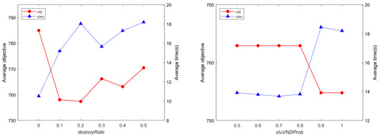
Figure 2.
Solution quality for different parameter settings.
To preserve a good balance between computation time and solution quality, we further tested the algorithm performance on the stop criterion parameter , which directly affected the global convergence of the algorithm. The algorithm was constructed using the optimal parameter settings defined above, while varying the maximum number of iterations without improvement, as shown in Figure 3. It can be observed that there was almost a linear relationship between the computation time and the number of iterations, achieving a significant improvement in solution quality in the first few seconds of execution. Therefore, the algorithm’s stopping criterion was set to 200 iterations without improvement. All subsequent experimental results in this paper were obtained using these optimal parameter values.
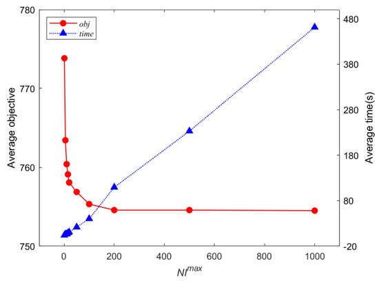
Figure 3.
Relationship between solution quality and the number of iterations without improvement (stopping criterion) for the testing instance set.
5.3. Characteristic Analysis of SDCVRPSC
To demonstrate the effects of customer-related costs, soft cluster conflicts, and split delivery at the cluster level on problem-solving, some instances were solved using the Gurobi and TLVND, respectively. Due to the large data scale of the benchmark instances, it was found in the pre-experiment that Gurobi had difficulty providing feasible solutions for all instances within one hour. Therefore, a performance comparison of Gurobi and TLVND was conducted on the testing instance set extracted during parameter tuning in Section 5.2. We recorded the best objective, , the lower bound, , the percentage gap between the best objective and the best lower bound, , and the number of instances solved to optimality provided by Gurobi within 3600s, while the best objective value, , and the calculation time, , obtained by TLVND, and the gap of solution quality between TLVND and Gurobi, , were recorded. The averages of each piece of data by instance category and corresponding numbers of customers are summarized in Table 7. However, Gurobi cannot find a feasible solution for some of the instances within the time limit. We exclude these instances from the optimality gap calculation in the corresponding group and provide the number of such instances (if any) next to each objective and optimality gap value. Note that Gurobi cannot provide any feasible solution and the average gap for the large instance, which is indicated by a ‘‘/” sign.
Table 7.
Comparison of Gurobi and TLVND on the testing instance set.
The experimental results demonstrate that TLVND can rapidly generate solutions that are comparable to or even superior to those provided by Gurobi, which also proves the rationality and effectiveness of the model and algorithm. Within the given 1 h time limit, Gurobi successfully solved three out of ten small-scale instances, but the average gap of feasible solutions found was still 21.93%, while TLVND achieved almost the same solution quality in only 5.18 s. Gurobi failed to provide any feasible solutions for a medium-scale instance, and the average gap of feasible solutions found was 55.91%, while TLVND provided solutions with better quality than Gurobi in only 13.19 s. More significantly, Gurobi failed to provide any feasible solutions for any large-scale instances, while TLVND obtained satisfactory solutions in only about 25 s. This was expected, as the solving time of Gurobi for NP-hard problems increased exponentially with problem size.
Due to the particularity of vehicle production, the number of parts suppliers is generally hundreds. Considering the business demand for rapid decision-making within minutes, the direct implementation of mathematical models on commercial solvers is insufficient to effectively solve SDCVRPSC, and heuristics that sacrifice optimality for computational efficiency can solve the problem in a reasonable time. In addition, in case of emergencies or changes in plans, heuristics can respond flexibly and generate solutions almost in real-time (i.e., on demand). Therefore, this further confirms the necessity of adopting heuristics to solve SDCVRPSC in the logistics of automotive parts.
5.4. Performance Evaluations
Since this paper is the first study of SDCVRPSC and no optimal solution is known, to facilitate the evaluation of algorithm performance, TLVND was compared with FFDDC_LKH and two-level VNS to verify the solution efficiency and solution quality of the algorithms on benchmark instances. The results of the five types of benchmark instances are shown in Table 8. The objective values obtained by the three algorithms were , where the best results were recorded as , and the percentage gaps between the best solutions obtained by the three algorithms and were counted: and the computation time . The best values are highlighted in bold.
Table 8.
Computational results for SDCVRPSC instances.
For different vehicle filling rates, the proposed TLVND always outperformed the two adapted heuristics in terms of solution quality. Although TLVND took longer to solve, it was only by about 5 min, and the maximum improvement in solution quality could reach 35.57%, which makes up for the time consumption and is highly valuable for business operations.
Furthermore, it can be observed that as the vehicle filling rate increased, the total cost showed a trend of decreasing first and then increasing. Specifically, as the vehicle filling rate increased, the transportation cost always decreased, but the penalty cost first decreased and then increased. To facilitate analysis, we illustrated the trends in the number of clusters, the vehicle capacity, the number of vehicles used, transportation cost, penalty cost, and the total cost comprising the two cost components at different vehicle filling rates, using the first instance from the benchmark as an example, as shown in Figure 4.
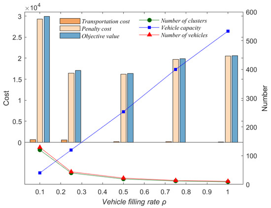
Figure 4.
Trends in the data for a case study at different vehicle filling rates.
Given that the vehicle capacity was set to the average demand of clusters, an increase in vehicle filling rate led to a decrease in the number of clusters, an increase in the number of customers within each cluster, and a rise in the average demand per cluster, thereby increasing vehicle capacity and decreasing the number of required vehicles to service the same customers and demands.
For the transportation cost, an increase in resulted in fewer vehicles visiting these customers, which also brought more opportunities for intra-cluster consolidation transportation. Consequently, more customers with similar direct shipment costs within the same cluster would be visited together, and except for the customer with the maximum direct shipment cost, all other customers only need to pay a much smaller drop cost, which reduces the transportation cost.
For the penalty cost, when the vehicle capacity remained constant and the number of clusters decreased, the time of inter-cluster transportation decreased, resulting in a corresponding decrease in penalty cost. When the number of clusters remained unchanged and the vehicle capacity increased, the opportunities for inter-cluster consolidation transportation increased and the penalty cost increased accordingly. Due to the synchronous increase in vehicle capacity and the number of customers in the cluster with the increase of , the distribution of customers in the cluster had a more significant impact on penalty costs when was small and the number of clusters was significantly reduced. In contrast, the significant increase in vehicle capacity had a more apparent impact on penalty costs when was large. Therefore, penalty costs showed a trend of first decreasing and then increasing under the interaction of vehicle capacity and the number of clusters.
5.5. Real Case Study
Considering that the SDCVRPSC is derived from automotive parts milk-run logistics with supplier cluster distribution in China, we further validated the performance of the proposed TLVND on real data collected from the case company (TPL) in its daily operation and analyzed the economic benefits brought by the algorithm in practical applications by comparing it with TPL’s expert decisions.
Three real-life cases were derived from TPL’s actual business scenarios in the Yangtze River Delta. The geographical distribution map of TPL’s depot and suppliers is shown in Figure 5, where each colored area represents a cluster, the blue flag represents the cluster center, the red flag represents the depot in Nanjing, and the red dots represent suppliers. For the three cases, the number of suppliers and clusters, the corresponding transportation plans provided by TPL’s experts, the transportation plans provided by TLVND, and the percentage gap in cost between the two plans are shown in Table 9.
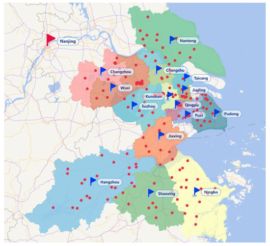
Figure 5.
Geographical distribution map of depot and suppliers in East China.
Table 9.
Comparison of TPL’s expert experience and TLVND on real cases.
In the above three cases, compared with transportation plans provided by TPL’s experts, TLVND achieved maximum savings of about 30%, which is quite considerable. These results confirm that our proposed method can offer a promising solution in addressing the realistic challenges faced by TPL. Considering that the rapid development of the automotive industry will further drive the demand for automotive parts, TLVND will bring a greater economic impact.
6. Conclusions
In this paper, we introduced a practical variant of the Clustered VRPs called SDCVRPSC, which has applications in automotive parts milk-run logistics with supplier cluster distribution. SDCVRPSC considers realistic settings such as the uncertain size relationship between cluster demand and vehicle capacity, split delivery to clusters, soft cluster conflicts, and customer-related costs. For SDCVRPSC, we provided an integer programming model and proposed the TLVND algorithm, which includes a two-stage construction, VND at both cluster and customer levels, and a perturbation mechanism. Experiments on designed SDCVRPSC benchmark instances demonstrated that TLVND performs more effectively than the commercial solver Gurobi and two adapted algorithms. In addition, the TLVND was especially customized for the special situation of the case company. The real case study results showed that the algorithm could effectively provide a solution to the problem and bring economic savings compared with expert experience in decision-making. The logistics department of the company has now integrated TLVND into its decision support system for practical use.
Furthermore, this work has the following limitations, which we hope to address in future research. The concept of milk-run has found diverse applications in supply chain logistics, leading to different milk-run patterns in practice. Therefore, the transportation problems in automotive parts milk-run logistics can incorporate more factors, such as heterogeneous vehicles, different geographical distributions of suppliers (uniform, clustered, or semi-clustered), and many attributes of VRP, including hard (soft) time windows and backhaul, to capture real-world scenarios. Future research work can consider other objectives, such as the load balancing of different vehicles, the payoff balancing of carriers, and carbon dioxide emissions; explore the possibility of exact algorithms, other metaheuristics, and the combination of TLVND with other heuristics; or study the integrated optimization of production, distribution, and inventory from the perspective of supply chain coordination.
Author Contributions
Conceptualization, R.X., Y.H. and W.X.; methodology, R.X., Y.H. and W.X.; software, R.X. and Y.H.; validation, W.X., Y.H. and R.X.; formal analysis, W.X.; investigation, R.X., Y.H. and W.X.; resources, R.X.; data curation, Y.H. and W.X.; writing—original draft preparation, Y.H.; writing—review and editing, W.X., Y.H. and R.X.; visualization, Y.H.; supervision, R.X. and W.X.; project administration, Y.H. and W.X.; funding acquisition, R.X. All authors have read and agreed to the published version of the manuscript.
Funding
This research was funded by the National Natural Science Foundation of China, grant number 62106098; the Stable Support Plan Program of Shenzhen Natural Science Fund, grant number 20200925154942002; and Guangdong Provincial Key Laboratory, grant number 2020B121201001.
Institutional Review Board Statement
Not applicable.
Informed Consent Statement
Not applicable.
Data Availability Statement
Not applicable.
Conflicts of Interest
The authors declare no conflict of interest.
References
- Svensson, G. The Impact of Outsourcing on Inbound Logistics Flows. Int. J. Logist. Manag. 2001, 12, 21–35. [Google Scholar] [CrossRef]
- Boysen, N.; Emde, S.; Hoeck, M.; Kauderer, M. Part logistics in the automotive industry: Decision problems, literature review and research agenda. Eur. J. Oper. Res. 2015, 242, 107–120. [Google Scholar] [CrossRef]
- Harrison, A. Perestroika in automotive inbound. Manuf. Eng. 2001, 80, 247–251. [Google Scholar] [CrossRef]
- Hosseini, S.D.; Shirazi, M.A.; Karimi, B. Cross-docking and milk run logistics in a consolidation network: A hybrid of harmony search and simulated annealing approach. J. Manuf. Syst. 2014, 33, 567–577. [Google Scholar] [CrossRef]
- Mao, Z.; Huang, D.; Fang, K.; Wang, C.; Lu, D. Milk-run routing problem with progress-lane in the collection of automobile parts. Ann. Oper. Res. 2019, 291, 657–684. [Google Scholar] [CrossRef]
- Meyer, A.; Amberg, B. Transport concept selection considering supplier milk runs—An integrated model and a case study from the automotive industry. Transp. Res. Part E Logist. Transp. Rev. 2018, 113, 147–169. [Google Scholar] [CrossRef]
- Ranjbaran, F.; Kashan, A.H.; Kazemi, A. Mathematical formulation and heuristic algorithms for optimisation of auto-part milk-run logistics network considering forward and reverse flow of pallets. Int. J. Prod. Res. 2019, 58, 1741–1775. [Google Scholar] [CrossRef]
- Sadjadi, S.J.; Jafari, M.; Amini, T. A new mathematical modeling and a genetic algorithm search for milk run problem (an auto industry supply chain case study). Int. J. Adv. Manuf. Technol. 2008, 44, 194–200. [Google Scholar] [CrossRef]
- Wu, Q.; Wang, X.; He, Y.; Xuan, J.; He, W. A robust hybrid heuristic algorithm to solve multi-plant milk-run pickup problem with uncertain demand in automobile parts industry. Adv. Prod. Eng. Manag. 2018, 13, 169–178. [Google Scholar] [CrossRef]
- Barthélemy, T.; Rossi, A.; Sevaux, M.; Sörensen, K. Metaheuristic approach for the clustered vrp. In Proceedings of the EU/MEeting: 10th Anniversary of the Metaheuristics Community-Université de Bretagne Sud, Lorient, France, 3 June 2010. [Google Scholar]
- Pop, P.C.; Kara, I.; Marc, A.H. New mathematical models of the generalized vehicle routing problem and extensions. Appl. Math. Model. 2012, 36, 97–107. [Google Scholar] [CrossRef]
- Battarra, M.; Erdoğan, G.; Vigo, D. Exact algorithms for the clustered vehicle routing problem. Oper. Res. 2014, 62, 58–71. [Google Scholar] [CrossRef]
- Marc, A.H.; Fuksz, L.; Pop, P.C.; Dănciulescu, D. A novel hybrid algorithm for solving the clustered vehicle routing problem. In International Conference on Hybrid Artificial Intelligence Systems; Springer: Berlin/Heidelberg, Germany, 2015. [Google Scholar]
- Vidal, T.; Battarra, M.; Subramanian, A.; Erdogˇan, G. Hybrid metaheuristics for the Clustered Vehicle Routing Problem. Comput. Oper. Res. 2015, 58, 87–99. [Google Scholar] [CrossRef]
- Expósito-Izquierdo, C.; Rossi, A.; Sevaux, M. A Two-Level solution approach to solve the Clustered Capacitated Vehicle Routing Problem. Comput. Ind. Eng. 2016, 91, 274–289. [Google Scholar] [CrossRef]
- Defryn, C.; Sörensen, K. A fast two-level variable neighborhood search for the clustered vehicle routing problem. Comput. Oper. Res. 2017, 83, 78–94. [Google Scholar] [CrossRef]
- Hintsch, T.; Irnich, S. Large multiple neighborhood search for the clustered vehicle-routing problem. Eur. J. Oper. Res. 2018, 270, 118–131. [Google Scholar] [CrossRef]
- Horvat-Marc, A.; Fuksz, L.; Pop, P.C.; Dănciulescu, D. A decomposition-based method for solving the clustered vehicle routing problem. Log. J. IGPL 2017, 26, 83–95. [Google Scholar] [CrossRef]
- Pop, P.C.; Fuksz, L.; Marc, A.H.; Sabo, C. A novel two-level optimization approach for clustered vehicle routing problem. Comput. Ind. Eng. 2018, 115, 304–318. [Google Scholar] [CrossRef]
- Xu, R.; Guo, R.; Jia, Q. A Novel Hybrid Metaheuristic for Solving Automobile Part Delivery Logistics with Clustering Customer Distribution. IEEE Access 2019, 7, 106075–106091. [Google Scholar] [CrossRef]
- Hintsch, T.; Irnich, S. Exact solution of the soft-clustered vehicle-routing problem. Eur. J. Oper. Res. 2019, 280, 164–178. [Google Scholar] [CrossRef]
- Aerts, B.; Cornelissens, T.; Sörensen, K. The joint order batching and picker routing problem: Modelled and solved as a clustered vehicle routing problem. Comput. Oper. Res. 2020, 129, 105168. [Google Scholar] [CrossRef]
- Hintsch, T. Large multiple neighborhood search for the soft-clustered vehicle-routing problem. Comput. Oper. Res. 2020, 129, 105132. [Google Scholar] [CrossRef]
- Islam, A.; Gajpal, Y.; ElMekkawy, T.Y. Hybrid particle swarm optimization algorithm for solving the clustered vehicle routing problem. Appl. Soft Comput. 2021, 110, 107655. [Google Scholar] [CrossRef]
- Li, S.; Wu, W.; Ma, X.; Zhong, M.; Safdar, M. Modelling medium- and long-term purchasing plans for environment-orientated container trucks: A case study of Yangtze River port. Transp. Saf. Environ. 2022, 5. [Google Scholar] [CrossRef]
- Hussain, I.; Wang, H.; Safdar, M.; Ho, Q.B.; Wemegah, T.D.; Noor, S. Estimation of Shipping Emissions in Developing Country: A Case Study of Mohammad Bin Qasim Port, Pakistan. Int. J. Environ. Res. Public Health 2022, 19, 11868. [Google Scholar] [CrossRef] [PubMed]
- Chen, L.; Chen, Y.; Langevin, A. An inverse optimization approach for a capacitated vehicle routing problem. Eur. J. Oper. Res. 2021, 295, 1087–1098. [Google Scholar] [CrossRef]
- Dantzig, G.B.; Ramser, J.H. The Truck Dispatching Problem. Manag. Sci. 1959, 6, 80–91. [Google Scholar] [CrossRef]
- Reichhart, A.; Holweg, M. Co-located supplier clusters: Forms, functions and theoretical perspectives. Int. J. Oper. Prod. Manag. 2008, 28, 53–78. [Google Scholar] [CrossRef]
- Dror, M.; Trudeau, P. Savings by Split Delivery Routing. Transp. Sci. 1989, 23, 141–145. [Google Scholar] [CrossRef]
- Dror, M.; Trudeau, P. Split delivery routing. Nav. Res. Logist. 1990, 37, 383–402. [Google Scholar] [CrossRef]
- Archetti, C.; Savelsbergh, M.W.P.; Speranza, M.G. Worst-Case Analysis for Split Delivery Vehicle Routing Problems. Transp. Sci. 2006, 40, 226–234. [Google Scholar] [CrossRef]
- Fu, L.-L.; Aloulou, M.A.; Triki, C. Integrated production scheduling and vehicle routing problem with job splitting and delivery time windows. Int. J. Prod. Res. 2017, 55, 5942–5957. [Google Scholar] [CrossRef]
- Archetti, C.; Speranza, M.G.; Savelsbergh, M.W.P. An Optimization-Based Heuristic for the Split Delivery Vehicle Routing Problem. Transp. Sci. 2008, 42, 22–31. [Google Scholar] [CrossRef]
- Sevaux, M.; Sörensen, K. Hamiltonian paths in large clustered routing problems. In Proceedings of the EU/MEeting 2008 Workshop on Metaheuristics for Logistics and Vehicle Routing, EU/ME, Athens, Greece, 1 October 2008. [Google Scholar]
- Ghiani, G.; Improta, G. An efficient transformation of the generalized vehicle routing problem. Eur. J. Oper. Res. 2000, 122, 11–17. [Google Scholar] [CrossRef]
- Lin, S.; Kernighan, B.W. An Effective Heuristic Algorithm for the Traveling-Salesman Problem. Oper. Res. 1973, 21, 498–516. [Google Scholar] [CrossRef]
- Helsgaun, K. An effective implementation of the Lin–Kernighan traveling salesman heuristic. Eur. J. Oper. Res. 2000, 126, 106–130. [Google Scholar] [CrossRef]
- Johnson, D.S. Near-Optimal Bin Packing Algorithms; Massachusetts Institute of Technology: Cambridge, MA, USA, 1973. [Google Scholar]
- Christofides, N. The Shortest Hamiltonian Chain of a Graph. SIAM J. Appl. Math. 1970, 19, 689–696. [Google Scholar] [CrossRef]
- Vidal, T. Hybrid genetic search for the CVRP: Open-source implementation and SWAP* neighborhood. Comput. Oper. Res. 2021, 140, 105643. [Google Scholar] [CrossRef]


Disclaimer/Publisher’s Note: The statements, opinions and data contained in all publications are solely those of the individual author(s) and contributor(s) and not of MDPI and/or the editor(s). MDPI and/or the editor(s) disclaim responsibility for any injury to people or property resulting from any ideas, methods, instructions or products referred to in the content. |
© 2023 by the authors. Licensee MDPI, Basel, Switzerland. This article is an open access article distributed under the terms and conditions of the Creative Commons Attribution (CC BY) license (https://creativecommons.org/licenses/by/4.0/).