Abstract
Unlocking the secrets of habitable urban areas is crucial to improve the quality of life for urban dwellers. Accurate assessment of the ever-changing dynamics of a modern metropolis remains a challenging task. Previous studies have failed to reveal the dynamics of urban building spatial configuration at the micro-level. By analyzing high-resolution satellite imagery, this study has developed new direct and indirect metrics to better understand building density dynamics. We also applied these metrics to a study area located in Nanning City, China, revealing fascinating insights into the evolving spatial patterns of building density over the past 17 years. Our Q/R analysis uncovered areas with high habitability and suggested strategic improvements for sustainable building spatial configuration. This study is a valuable addition to the growing body of urban development research and provides scientific references for measurements of sustainable urban planning worldwide.
1. Introduction
Building density (BD) is a quantitative indicator that reflects the degree of building occupation on a plot of land. It is of great significance to land use, urban planning, and human settlements. In recent years, advances in remote sensing and earth observation techniques have revolutionized the study of building density.
In the 1970s, the European Joint Research Center (JRC) used the GHSL project (Global Human Settlement Layer, GHSL) to provide GHSL building density mapping products for Europe and North America after 1975 [1,2,3]. The development of satellite imaging technology has enabled the GHSL project to effectively map spatio-temporal patterns and characteristics of urban buildings, forming the basis for its success in producing building density mapping datasets [4,5]. This approach has replaced traditional methods relying on investigations of historical maps of cities.
Building density adjustments have been widely implemented in numerous Asian cities, including downtown areas and residential neighborhoods, to address the issue of urban land scarcity. Tall buildings and apartment complexes have become increasingly prevalent in cities such as Hong Kong, Tokyo, Singapore, Shanghai, Taipei, Beijing, Kuala Lumpur, Seoul, and others. In China, several researchers have explored the applicability of GHSL BD mapping products, such as Wang et al., who established a model to estimate urban building density in China’s five typical cities [6,7], and Huang et al., who proposed a new kernel building density model to quantify the relationship between building density and heat island effect [8]. Dong et al. also extended the scope of building density [9] from an index that quantitatively represents the conditions of building occupancy to a set of eight quantitative metrics to measure building density from different aspects [9]. These studies represent frontier studies on building density quantification.
Many states around the world have implemented building density regulations, such as restrictions on lot size zoning, building size, and/or floor area ratio, based on study results that revealed negative environmental and social impacts. Building density measurements have largely been driven by practical urban planning needs, but attention has shifted towards digitizing and quantifying the urban design, shape, and spatial configuration in response to the idea of a habitable city. Building density is closely linked to various aspects of human settlements, such as urban temperature [10,11,12], urban ventilation [13,14,15,16], indoor comfort (noise, light) [17], air pollution and PM2.5 concentration [18], and even residents’ health [17]. As a result, it remains an essential focal point in urban studies.
With the emergence of new earth observation techniques, BD investigations previously depending on ground measurement can now be done more efficiently and continuously using remote sensing and GIS techniques. Building density remote sensing (BDRS) has brought four major developments to BD study—data source, data processing, application, and data visualization, which are also the representative characteristics of BDRS:
- (1)
- Data sources: Today, there are more options for remote sensing platforms, satellite images, spatial resolutions, spectral resolutions, and sensing time due to the increase and improvement in remote sensing platforms and satellite sensors. High-resolution satellite images have become one of the major data sources for BD studies [19,20,21,22,23], and global satellite image data platforms and big data cloud computing platforms (such as Google Earth Engine) have diversified the data sources for BD studies [24].
- (2)
- Data processing: As new BD problems and aims emerge, the need for quantitative analysis has significantly risen, leading to the proposal of new data analysis methods and models. For example, Huang et al. proposed a kernel building density model, where the building density at a circle region is the ratio of the total building area to the circle area [8]. Based on this model, the building density can be measured at different sizes.
- (3)
- Application: BD study is no longer just about urban land use evaluation but also serves various functions, including analyzing urban temperature [10,11,12], ventilation [13,14,15,16], and other urban issues, such as indoor comfort conditions (noise, light) [17], air pollution and PM2.5 concentration [18], and residents’ health [17]. BD mapping plays an important role in these applications [6], such as gridded Germany population mapping based on the data of building density, height, and type [25], mapping of urban features using TanDEM-X and Sentinel-2 satellite data [26], the upgrading of global urban DEM using building density data [27], etc. These are all the new developments in the study of building density.
- (4)
- Data visualization: Urban development today requires not only a one-time investigation but also the dynamics, namely, various quantitative information on BD changes; for example, LiDAR and GEOBIA data can be used to measure spatial-temporal changes in 3D building density [28]; high-resolution images can analyze changes in building density in Shanghai [21], and high-resolution multi-view satellites can observe subtle changes in China’s megacities [29]. However, few studies have been reported in this field.
Previous studies on building density have relied mainly on simplistic measurements, with no comprehensive quantitative measurement framework available. Additionally, identifying building shape features requires high-resolution satellite imagery, which is not free for public use. Due to the high cost of image acquisition, studies on building density remain rare. Quantitative evaluation of habitability within a city facilitates the identification of urban problems and targeted improvements to the environment. However, it is an extremely complex procedure, and only a few applications and practical models have been proposed for micro-scale applications. Previous studies have mostly been limited to static assessments for a particular phase, making it difficult to reveal the dynamics of cities at the micro-level.
In this study, we proposed two categories of thirteen models to investigate the changes in building density and dynamics of the study area in Qingxiu District of China’s Nanning City Using high-resolution satellite images. We also assessed the habitability of the study area to provide new scientific references for the development of an ecologically unique city in Nanning. Based on remote sensing techniques, our primary aim was to discover macro trends (spatial and temporal changes) and reveal the macro dynamics of Nanning City. Based on our results, residents can identify areas with reasonable habitability in the urban area. Our research can provide a general guidance to facilitate the public’s understanding of the habitability of the city and help them choose a suitable place to reside. It could also serve as a reference for the government to evaluate urban development.
2. Methods and Data Sources
2.1. Study Scheme and the Main Elements
This study aimed to establish a remote sensing-based quantitative method for the quick identification of urban habitable areas. The research scheme consisted of two parts: a theoretical and an application part. The theoretical part combined proposed theoretical models with technical studies. This study first proposed a set of metrics for building density measurement and obtained the dynamics of building density based on time series of high-resolution satellite images. It then investigated the changing trends and impacts on the urban environment. Based on these findings, the proposed methods were applied to the habitability evaluation of the study area. The flowchart of the research scheme is shown in Figure 1.
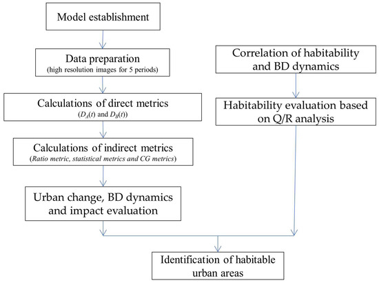
Figure 1.
Research scheme and technical roadmap for the entire study; variables used in the figure include the following: building areal density DA(t), building number density DB(t), ratio metric DA/B(t), and CG statistical metrics MA, MB, and MA/B, as well as impetus Ii~j.
2.2. Models for Building Density Measurement
2.2.1. Direct Metrics
There are two direct metrics for building density measurement: building areal density DA(x, y, t) and building number density DB(x, y, t). These can be directly obtained via direct measurement. DA(x, y, t) is the ratio of building area to unit size, indicating the degree of building coverage or building occupancy rate within a certain area. DB(x, y, t) is the number of buildings in a given unit area. Both can be calculated as follows:
where S represents the total area of the study area; SA(x, y, t) represents the total building area in the study area; and NA(x, y, t) represents the number of buildings in the study area. Both SA(x, y, t) and NA(x, y, t) were obtained using remote sensing techniques. The parameters x, y denote spatial coordinates, while t indicates the specific time considered for measuring building density.
DA(x, y, t) = SA(x, y, t)/S
DB(x, y, t) = NA(x, y, t)/S
2.2.2. Indirect Metrics
Indirect metrics are obtained by reanalyzing the direct features. Here we proposed several indirect metrics, including the ratio of the total area and the corresponding number of buildings, 7 statistical indices, and 4 measurements of the changes in the center of gravity (CG metric). These metrics also vary with time (t).
- (1)
- Ratio metric
The ratio metric is defined as the ratio of DA(x, y, t) and DB(x, y, t):
DA/B(x, y, t) = DA(x, y, t)/DB(x, y, t)
It is the ratio of building areal density and building number density.
By integrating Equations (1) and (2), Equation (3) can be modified as follows:
where DA/B(x, y, t) represents the ratio of building areal density and building number density. A lower value denotes a relatively large number of buildings in the study area, suggesting that most of the buildings are small and compact. Conversely, a higher value suggests a relatively small number of buildings in the study area, indicating most of the buildings are bulk ones. Since DA/B(x, y, t) captures dual measurements of both building areal density DA(x, y, t) and building number density DB(x, y, t), it can better display the spatio-temporal variations than if it only considered the individual building densities of DA(x, y, t) or DB(x, y, t). In addition, analysis based on the ratio metric further suggests that this index is an important measurement for evaluating the habitability of urban areas.
DA/B(x, y, t) = SA(x, y, t)/NA(x, y, t)
To visualize the status of DA(x, y, t*), DB(x, y, t*), and DA/B(x, y, t*) at time t*, a contour map can be created corresponding to the time t*. These values can be simplified to DA(t*), DB(t*), and DA/B(t*), which can further be reduced to just DA, DB, and DA/B without considering the time factor.
- (2)
- Statistical metrics
The statistical metrics include mean values MA, MB, and MA/B, mean square deviation SDA, SDB, and SA/B, correlation coefficient rA-B, as well as the intercept a and slope b from the regression equation DA = f(DB), where MA, MB, MA/B can be calculated as follows:
In the formula, M and N represent the image matrix’s row and column numbers, respectively. When x represents DA, DB, and DA/B, respectively, its corresponding mean value can be expressed as Mx. The root mean square error (RMSE) can be computed accordingly as follows:
Here, the M, N are the same as in Formula (5).
For the intercept and slope in the regression equation DA = f(DB), we can get it as follows:
where a and b are the intercept and slope of the regression equation, respectively.
DA = a + bDB
- (3)
- CG metrics
Changes in the center of gravity (CG) can depict variations in building spatial distribution. In this study, we adopted the concept of CG from physics and geometry. The objective was to convert the two-dimensional CG of building spatial distribution into the CG’s spatial-temporal trajectory, which describes the overall spatio-temporal changes in building locations over the past 17 years. To accomplish this, we needed to determine the position of the CG and delineate its trajectory. Here we developed a fast algorithm by combining the image pixel matrix of the study area to obtain the location of the CG as P(X, Y):
Here, fmn represents the BD value for the pixel location (m, n), while comprises three statistical metrics MA, MB, and MA/B, which can be computed using Equation (5). For instance, if we use an image matrix with a size (M = 10, N = 13), by replacing fmn with equations DA, DB, and DA/B, respectively, each CG metric for the three different statistical measurements at different time can be obtained.
The characteristics of CG changes include distance moved, direction of movement, and movement speed. The distance moved (Li~j) is the length of the CG’s movement from its position (i, j) at time yi (year) to its new position (i + 1, j + 1) at time yi+1 (year). The direction (θ) of movement is the direction of the CG moving from the previous location (i, j) at time yi (year) to the new location (i + 1, j + 1) at time yi+1 (year), although the measurement of the direction of movement was not used here. The speed of movement vi~j is the ratio of Li~j to the time interval yi+1-yi:
vi~j = Li~j/(yj − yi)
On the base of the Equation (5), moving speed vi~j at different periods can be computed.
Impetus is a dynamic parameter used in this study to quantitatively describe the intensity of BD changes. The CG’s impetus serves as an index and its corresponding formula is as follows:
Ii~j = Mxvi~j
Here, Mx represents the density value at P(X, Y) under building density metric x, where x could be DA, DB, or DA/B. When x is used as DA, DB, or DA/B, the corresponding Mx is the mean value of MA, MB, or MA/B, respectively. Ii~j and vi~j are, respectively, the impetus and velocity of P(X, Y) moving from the time yi (year) to the time yi+1 (year).
2.3. Habitability Evaluation Based on Q/R Analysis
Building habitability refers to the degree or level of comfort, safety, and livability of a building or structure [10,11]. A habitable building provides a healthy, comfortable living or working environment for occupants, with adequate ventilation, lighting, and protection from environmental hazards like noise pollution, air pollution, and natural disasters. Building habitability is a critical consideration in urban planning and development for creating sustainable, resilient, and livable cities. Environmental factors such as temperature, ventilation, noise, and illuminance, which are closely related to BD, often affect the habitability of a city. Therefore, analyzing the spatio-temporal distribution of DA/B, which contains information on both DA and DB, can help determine the habitability of a city. On the basis of the spatio-temporal distribution of DA/B, here we proposed a habitability evaluation method using Q/R analysis.
According to the definition of DA/B and Equation (4) provided in Section 2.2.2, the building spatial pattern corresponding to a low value of DA/B is referred to as an R-type building configuration, whereas the building spatial pattern corresponding to a high value of DA/B is called a Q-type building configuration. A small value of DA/B represents a large number of small and compact buildings, while a high value of DA/B corresponds to a small number of sparse and large buildings, as suggested in Section 2.2.2. We express these observations using the Q/R combination provided in Table 1.

Table 1.
Habitability evaluation based on Q/R analysis.
For simplification, we classified SA and NA into H/L classes instead of numerical values, resulting in four possible combinations (as shown in Table 1). If we integrate the four results into Equation (4), we obtain only two DA/B results, which are represented by H/L values. In the “Type” row, we used R-type and Q-type to define the corresponding categories of DA/B. It can be concluded that only column 2 belongs to the Q-type category, suggesting buildings with this configuration are habitable, while the other three options are all in the R-type category, suggesting that buildings with these three combinations are probably not habitable.
Table 1 shows a clear relationship between building spatial configuration and the mathematical model for the Q-type building configuration based on Equation (4). The habitable condition only holds when SA has an H value and NA has an L value, denoting that only buildings with spacious rooms and sufficient open outdoor environments are more habitable, while the R-type buildings have no such correspondence. Specifically, the Q-type buildings must meet at least the following four criteria:
- ①
- Low heat island effect;
- ②
- Adequate ventilation;
- ③
- Low noise and light pollution;
- ④
- Low solid waste and air pollution.
These rules are the prerequisites for a habitable urban area.
2.4. Information Extraction and Building Density Mapping
2.4.1. The Study Area
This study focused on a rectangular urban area (between 108°20′00″~108°20′48″ E and 22°49′08″~22°49′39″ N) in the middle of Qingxiu District, Nanning City of China’s Guangxi Province, as shown in Figure 2. This study investigated the dynamics in building density within the 1.3 km2 study area, which primarily consists of dense urban buildings and newly built blocks. The three-dimensional enlargement of the study area is shown in Figure 3. The study area has undergone fast upgradation of old buildings over the past decades. The study area is divided into six parts by two major NE-directed roads and two major NW-directed roads, with numerous smaller streets further segmenting each part (as shown in Figure 4). The building distribution in the new urban area is relatively organized, whereas the old urban area exhibits more disorganization. Notably, there are no lakes, rivers, or forests in the study area. This representative study area exemplifies Nanning’s rapid urban development over the past 30 years. It also represents the typical development process of most Chinese cities in the 21st century.
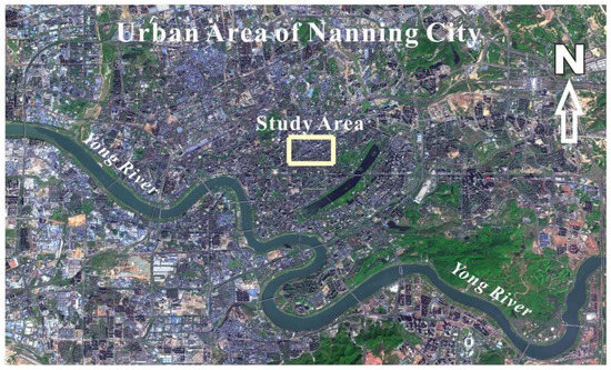
Figure 2.
Geographical configuration of the study area and its surrounding urban areas in the Nanning-based QuickBird-2 high-resolution images.
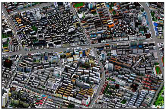
Figure 3.
A three-dimensional view of the spatial distribution of buildings in the study area.
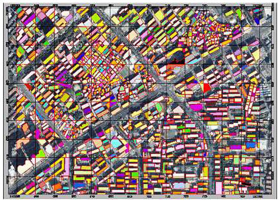
Figure 4.
Scheme for image matrix design with grid size Δx = Δy = 100 m and total row and column numbers of 10 and 13, respectively.
2.4.2. Building Density Mapping
In this study, we used the QuickBird-2 high-resolution images obtained on 13 October 2002, 16 November 2007, 11 February 2019, 4 November 2013, and 24 October 2019 to map changes in building density over the past 17 years. After performing image geometric correction and enhancement, we created an image matrix with a block size of Δx = Δy = 100 m, consisting of 10 rows and 13 columns (as shown in Figure 4). Using the measurement method outlined in Figure 4, we calculated DA and DB for each grid and established the two-dimensional matrixes for DA(tn) and DB(tn) for the five periods (n = 2002, 2007, 2009, 2013, 2019). Here, DA and DB represent the total building area and the number of buildings in a given grid, respectively. If a building is partially located within a grid, the number of the building is its areal proportion within the grid, with a range of 0.0~1.0 (Figure 5).
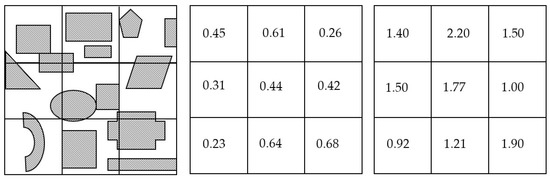
Figure 5.
Measurement scheme for the direct metrics of building areal density DA and building number density DB. Left: building spatial distribution against grid configuration; middle: matrix for building area density DA; right: matrix for building number density DB.
2.4.3. Visualization of Building Density Changes
Using the methods proposed in the previous section, we generated contour maps of DA(tn), DB(tn), and DA/B(tn) for different periods (n = 2002, 2007, 2009, 2013, and 2019) (Figure 6). The figures clearly illustrate the spatial changes in building density over time.
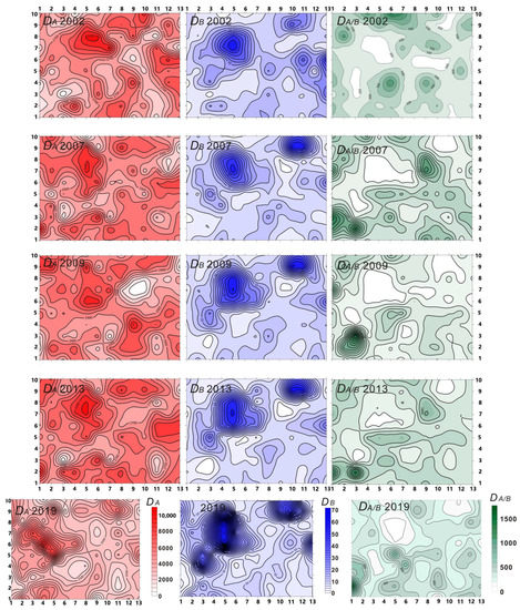
Figure 6.
Contour maps of DA, DB, and DA/B for the five periods (2002, 2007, 2009, 2013, and 2019); red ones are the contour map of DA, blue ones are the contour map of DB, and green ones are the contour map of DA/B. Legends for the three densities are shown in their results of 2019.
The contour maps for the three building densities in Figure 6 revealed that the overall changes in DA and DB over the past 17 years have similar spatio-temporal characteristics, that is, with high-value areas located in the blocks surrounded by the major roads. The distribution of DB is similar to that of DA. Additionally, there have also been some changes in the spatial distribution of both variables over the past 17 years, but the changes are not clearly evident on the contour maps. Therefore, further quantitative analysis is needed to investigate such changes.
3. Results
3.1. Changes Based on Direct Metrics
The mean is an essential statistical concept that reflects the central tendency of the building density. We generated histograms for MDA and MDB for their corresponding five periods (Figure 7). It can be seen that MDA changed with small fluctuations over the 17 years from 2002 to 2019 but showed a slight overall increasing trend. The MDA in 2019 was 3500.87, which is much higher than that of 2022 (MDA = 2921.70), with an increase of approximately 19.82%. Thus, it can be inferred that urban building areas have achieved significant development over the past 17 years. MDB showed a steady, increasing trend and peaked at 13.19 in 2019. The value of MDB in 2019 is 7.11 higher than that in 2002 (MDB = 6.08), or equivalent to a 116.94% of increase over the 17 years. Therefore, it also reflects rapid development in the urban buildings in the study area over the past 17 years in terms of the number of buildings.

Figure 7.
Historical changes in MDA and MDB over the past 17 years.
3.2. Changes Based on Indirect Metrics
The statistical characteristics were measured based on the metrics, including mean values MA, MB, and MA/B, mean square deviation SDA, SDB, and SA/B, correlation coefficient rA-B, as well as the intercept a and slope b from the regression equation DA = f(DB).
- (1)
- MA/B(t)
MA/B(t) represents the mean value of building area DA/B(t). The MA/B(t) changing trend was depicted in Figure 8. It can be seen from Figure 8 that MA/B(t) initially displayed a decreasing trend from 2002 to 2007, followed by a long decreasing trend from 2007 to 2019. In 2019, the MA/B(t) value (543.46) compared to that in 2002 has dropped by approximately 15.2%. Based on the definition of MA/B(t) in equation (4), the changes in MA/B(t) suggested that the upgraded buildings have developed from small and compact buildings to sparse and voluminous buildings. Therefore, a higher MA/B(t) indicates that the urban building configuration is more reasonable and habitable, while a lower MA/B(t) suggests the opposite. Figure 8 revealed that the influence of the building spatial configuration in the study area on habitability has fluctuated over the past 17 years. It used to be in better condition in 2007–2009 but has slightly decreased since then. It is worth noting that more attention should be paid to this aspect in future urban planning.
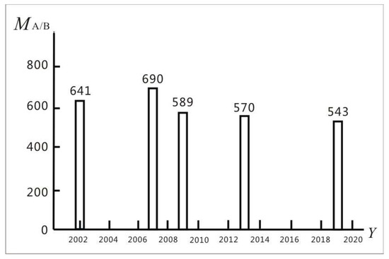
Figure 8.
Historical change of MA/B from 2002 to 2019. MA/B(t) initially displayed a decreasing trend from 2002 to 2007, followed by a long decreasing trend from 2007 to 2019.
- (2)
- SDA(t), SDB(t) and SA/B(t)
The RMSE is a commonly used measurement of the differences between values predicted by a model and the values observed. In this study, SDA(t), SDB(t), and SA/B(t) are the RMSE for DA, DB, and DA/B, respectively, to examine the degree of dispersion in the changes of the three building densities. Regarding the difference in the role of the statistical metrics, the changes in SDA(t), SDB(t), and SA/B(t) also imply meanings. A high value reflects that the urban buildings in the study area have great differences and diversity in size and shape and thus are able to provide a better building pattern and higher habitability. Conversely, a low value reflects small differences in buildings, resulting in monotony in spatial configuration and a lack of habitability for residents. From this, we analyzed the changes in the three RMSEs over the past 17 years.
SDA(t): SDA(t) fluctuated slightly from 2002 to 2013 and then increased significantly from 2013 to 2019. In 2019, it reached 1638.61, which is 467.93 (~40%) higher than in 2002 (1170.68), reporting a large change in urban building area density—including greater diversity in building size. The building spatial configuration has also undergone significant changes, and the new building spatial pattern is more inhabitable.
SDB(t): The overall trend of SDB(t) is quite similar to SDA(t). Its value in 2019 (12.54) is 7.41 (~144.4%), higher than that in 2002 (5.13). There has been a substantial increase in SDB(t) from 2013 to 2019, implying that a dramatic change in the number of buildings has happened too. Therefore, regarding the number of buildings, it revealed that the spatial configuration of buildings has undergone significant changes. It also suggested that the new building spatial pattern is more inhabitable.
SA/B(t): The change in SA/B(t) over the past 17 years is dramatically different from the trends of SDA(t) and SDB(t). It does not just show a steady rise or fall, but instead starts with an initial increase from 2002 to 2007, followed by a stable status from 2007 to 2009, and then ends with a decreasing trend from 2009 to 2019. Overall, SA/B(t) changed from 2002 (354.66) to 2019 (199.85), with a drop of 43.65%. According to the explanation in Formula (4), the changes in SA/B(t) revealed that the buildings in the study area have developed from small and compact buildings to large and sparse buildings. This provides quantitative evidence of the consistent improvement in building spatial configuration, towards a more habitable future (Figure 9).
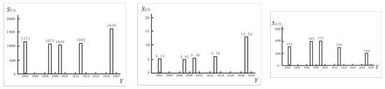
Figure 9.
Historical changes of SDA, SDB and SA/B from 2002 to 2019.
- (3)
- DA—DB regression analysis
The slope and intercept of the regression equations for the five periods are shown in Equation (11) and Figure 10. It can be seen that the slope b(t) has generally shown a decreasing trend from 2002 (128.55) to 2019 (69.35), with a relative drop of 46%, indicating that the impact of DB on DA is statistically decreasing over time. The intercept values a(t), varying between 2100 and 2600, are of little significance in this study.
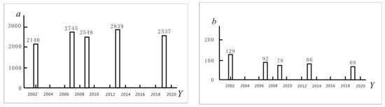
Figure 10.
Variations in intercept (a) and slope (b) of the DA-DB regression equations for the five periods.
- (4)
- Correlation analysis
The correlation coefficients rDA—DB between DA-DB for the five periods are plotted in Figure 11. Overall, the year 2009 marked a turning point in the coefficient change, with the correlation coefficient decreasing from 2002 to 2009 and subsequently increasing from 2009 to 2019. This suggests that rDA—DB is not constant but changes with building spatial pattern development.
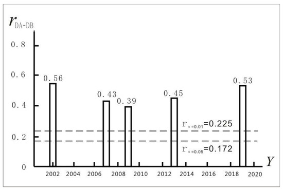
Figure 11.
The DA—DB correlation coefficient changes from 2002 to 2019.
A correlation test was also performed on rDA—DB. The thresholds of the correlation coefficient for a statistically significant correlation at significance levels α = 0.05 and α = 0.01 are α = 0.05 and α = 0.01 are rα=0.05 = 0.172 and rα=0.01 = 0.225, respectively. Based on the results in Figure 11, all correlation coefficients rDA—DB for DA-DB in the five periods are all much higher than the two thresholds. This indicates that during the period from 2002 to 2019, the correlation between DA and DB in the study area was in a significantly positive correlation at both significance levels of α = 0.05 and α = 0.01. The positive relation denoted that an increase in building area density happened concurrently with an increase in the number of buildings and vice versa.
3.3. CG Metrics
We obtained the CG coordinates of the three building densities in the five periods based on Formulas (8)–(10), as shown in Figure 12. However, in a small-scale map of the study area, it is difficult to depict the dynamics of the CG. Therefore, we have created an enlargement of the local area with the CG locations (Figure 13) to clearly describe the trajectories of the CG of the three densities over the past 17 years.
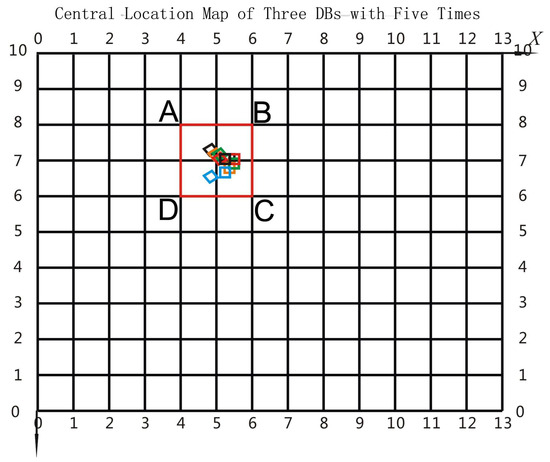
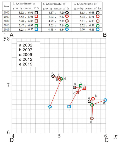
Figure 13.
The enlargement of the CG trajectory displayed in Figure 12.
Combining Figure 12 and Figure 13, it can be seen that over the past 17 years, the positions and trajectories of the CG of the three building densities have mainly been located in the mid-northwest part of the study area. This indicates that the spatio-temporal distribution of buildings in the study area is not uniform, which is a key characteristic of rapid urban development. Among the three CG clusters, the CG cluster of DB is in the most northwest direction, while the CG cluster of DA is arranged in the southeast, and the CG cluster of DA/B is located in the middle of the two clusters of DA and DB. These three CG clusters have different movement speeds, which reflect the spatio-temporal movement of the buildings in the study area and provide an essential reference for analyzing the overall changes in urban buildings.
The concept of impetus (I) is the product of an object’s mass (m) and its velocity (v). Here, impetus was used to measure the intensity of overall spatial changes in urban buildings. The higher the value of I, the greater the intensity and magnitude of changes in the buildings, providing an overall measurement of the magnitude of changes in the buildings. Using Equation (10), the impetus (I) of three BDs in five in periods is calculated, which is referred to as algorithm 1. As the CP moves from the previous location to the next, the density and speed of the CP also changes. Therefore, the calculation of impetus must consider these changes accordingly. The corresponding calculation method is established in Figure 14 and Equation (12), which is referred to as algorithm 2.
Ii = 0.25(Mi + Mi+1)(vi + vi+1)
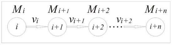
Figure 14.
Scheme of the calculation of the impetus (I) based on building changes (m) and (v).
The changes in impetus (I) for the three BDs over the past 17 years are shown in Figure 15. The figure shows that IDA has experienced two fluctuations with a low-high-low-high trend. The impetus (I) of IDB was still low until 2007, but it increased sharply after 2007, indicating that the DB has experienced a dramatic change during these periods after 2007. IDA/B was still high from 2002 to 2007, followed by a constant decrease since 2007, suggesting that the building spatial pattern has changed significantly after 2007, from densely populated small buildings to large and sparsely populated buildings. This change is consistent with the actual urban development in the study area. Therefore, based on the analysis of the impetus (I) of the three building densities of IDA, IDB, and IDA/B, the new observed conclusion and technical report on building dynamics can be valuable for the development of unique ecological cities and smart cities in Nanning.
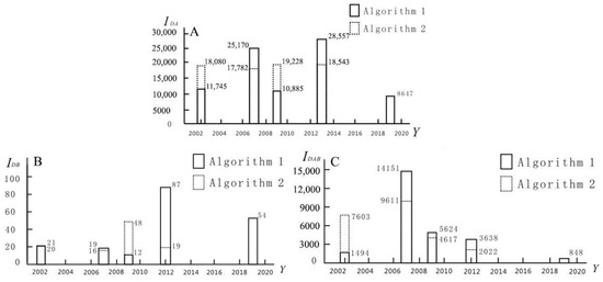
Figure 15.
Impetus (I) for the three BDs (IDA (A), IDB (B), and IDA/B (C)) over the past 17 years; the solid line is algorithm 1 and the dashed line is algorithm 2.
4. Applications
4.1. The Varied Building Density across Large Cities
Yu et al. [30] investigated building density in downtown Houston by analyzing high-resolution airborne LiDAR data. Compared to Nanning, the downtown area of Houston is characterized by a more complex urban landscape, where buildings and other man-made structures are densely concentrated. The building density in downtown Houston is more diverse as the urban economic, social, and cultural functions of various districts differ, leading to variations in building size, height, volume, density, morphological heterogeneity, and vertical roughness across districts. Using LiDAR data, they displayed the planimetric and horizontal density of buildings, as well as the 3D density of buildings. Similarly, the study results by Yan and Li [31] for Hong Kong also indicated that the building density in downtown Hong Kong is much higher than that in Nanning, and the situation is still worsening. Regarding the changes in building density, the situation in Nanning is better than in many other large Asian cities such as Hong Kong, Tokyo, Singapore, Shanghai, Taipei, Beijing, Kuala Lumpur, Seoul, and others [32,33].
The urban development in Nanning, as represented by building density, is quite different from that of other large Asian cities. In representative large Asian cities (i.e., Hong Kong, Shanghai, Beijing, Singapore, Tokyo), due to extremely limited land availability, high-density compact communities are often developed, which can compromise livability and quality of life [34]. However, Nanning’s city planning allows for a more balanced approach to urban development.
Building density is closely related to the ambient urban environment. Unreasonable building distribution can affect environmental conditions such as ambient temperature, ventilation, noise, lighting, solid pollution, and air pollution, which can have a negative impact on the city’s habitability. In the context of an urban environment, service quality has been found to have a positive correlation with building density. The more compact a city is, the greater the degree of engagement between individuals and their surroundings [35]. However, high building density alone is not enough to ensure positive social interactions for daily activities like living, working, and recreation. To ensure a healthy and habitable community, it is crucial to evaluate how building density affects the urban environment through quantitative analysis [36].
4.2. Identification of Habitable Urban Areas
In this paper, the urban building areas that meet the aforementioned four rules are referred to as habitable areas. We used the Q/R analysis and the DA/B contour map to determine the extent of DA/B. According to Table 1, combined with the actual conditions in the study area, the areas with the contour lines DA/B ≥ 400 are regarded as habitable areas, such as Q1, Q2,…, and Q9, highlighted by boxes in Figure 16. Since this is only an initial delineation without in situ verification, it is also referred to as the initial habitable area. The regions that fail to meet the rules will be removed after in situ verification.
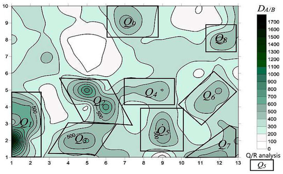
Figure 16.
Example of identification of habitable urban areas based on DA/B contour map of 2019; the initial delineations were highlighted using solid boxes, while after in situ verification, the regions that failed to meet the rules were highlighted using dotted boxes.
In situ surveys are an ideal way to identify fake habitable areas from the initial habitable areas. However, in situ surveys can be laborious. As an alternative, we used high-resolution satellite images to visually identify fake habitable areas. Here, the QuickBird-2 images obtained in 2019 were used as the base map, and the nine initial habitable areas were overlaid with the base map accordingly (Figure 17). Through visual interpretation, the building spatial patterns in each initial habitable area were analyzed to check if the combination of SA and NA values is a Q-type combination. A comparison of Figure 16 and Figure 17 revealed that the areas with high values in the DA/B contour map displayed a significant relationship with the combination of SA’s H value and NA’s L value. The high-value areas Q1, Q2, and Q8 are dominated by large buildings with spacious indoor rooms and sufficient open outdoor environments. Although major roads provided sufficient open outdoor environments for the ambient buildings, the traffic noise destroyed habitability, and thus they cannot be identified as habitable areas. The buildings in high-value areas Q3, Q4, Q5, Q6, and Q9 are large buildings with spacious indoor rooms and sufficient open outdoor environments, resulting in better ventilation and lighting, lower traffic noise, and less mutual interference between residents. These five areas should be classified as habitable areas (solid boxes). Based on this, the complex identification of habitable areas involves the delineation of the high-value areas of the DA/B contour map using remote sensing techniques, which can be implemented at large scales to identify habitable urban areas.
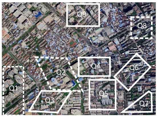
Figure 17.
Delineation of the habitable areas based on the QuickBird-2 high-resolution images obtained in 2019; the areas highlighted by dotted boxes were removed.
The data presented in Figure 16 and Figure 17 show that the buildings within the range of DA/B [0, 200] are primarily small and compact buildings. This finding aligns with the Q-type problem statement, which suggests that a small value of DA/B indicates a relatively large number of buildings with limited room space.
4.3. Limitations of the Current Study
The four proposed rules in Section 2.3 are based on satellite data without additional information about individual buildings (e.g., height, number of rooms, etc.). As a result, it is difficult to ascertain whether a building is a low and flat one or a high and compact one. Thus, our rules may not be applicable under certain conditions: for example, increased exposure of buildings and ground to sunlight could elevate heat island temperatures, while shaded areas reduce them. This means densely arranged low buildings could provide more shade, resulting in lower overall air temperature. Moreover, flat building profiles preserve wind flow overtop the buildings, while dispersed tall buildings create turbulence and reduce the overall wind speed. Unfortunately, in this study, the lack of information on building height in this study precluded us from considering this factor.
Here, some critical information about individual buildings (e.g., height, number of rooms, etc.) was not available for further evaluation based on the three-dimensional structures of the buildings. Future studies could consider using three-dimensional data on the spatial distribution of buildings as complementary data to overcome these limitations. Additionally, future approaches should aim to integrate building height into habitability evaluation. The methods proposed in this study can also be duplicated in other cities since they provide a simple and efficient way to delineate habitable urban areas using remote sensing techniques. However, several challenges may arise when applying these techniques to different cities, including a lack of data on building configurations in different cities or the fact that the study only focused on a specific urban area. Therefore, future research should collect and analyze data from various cities to understand how remote sensing techniques can accurately identify habitable urban areas across different geographical regions.
5. Conclusions
Understanding cities’ habitability facilitates the identification of urban problems and targeted improvements to the urban environment. Building Density serves as an important indicator of the spatio-temporal changes in building spatial configuration. This study proposed two categories of models based on high-resolution satellite images to measure building density dynamics. These include direct metrics such as building area density (DA) and building number density (DB), as well as indirect metrics such as the ratio of total area and the corresponding number of buildings, nine statistical indices, and six measurements of changes in the center of gravity. Using these metrics, we investigated the dynamics and changes in building density in Nanning, China, across five periods from 2002 to 2019, based on high-resolution satellite images. By examining the changes in building density over time, we can better understand how urban development has impacted the city’s habitability and identify areas that require intervention or further investigation.
This study has obtained the following key findings: over the past 17 years, MDA has changed with small fluctuations but has shown an overall slight increase, implying that urban building areas in the study period have undergone significant development. The changes in SA/B also revealed an evolution from small and compact structures to larger and more sparsely arranged buildings. This quantitative evidence suggests a consistent improvement in building spatial configuration and a more habitable future. Additionally, we analyzed the positions and trajectories of the three building density centers of gravity (CG), which describe the spatio-temporal movement of buildings in the study area. The observed trends in building dynamics provide valuable insights for the development of unique ecological cities in Nanning City. Furthermore, we have conducted a habitability evaluation based on Q/R analysis to identify habitable areas within the study area. The availability of reliable quantitative building density data will prove to be beneficial for examining the urban environment and facilitating the management of future urban land development and expansion projects.
Author Contributions
Conceptualization, Y.W., Z.J. and X.Y.; formal analysis, Y.W. and Z.J., and X.Y.; data curation, Z.J.; writing—original draft preparation, Y.W. and Z.J.; writing—review and editing, X.Y. and Y.W.; supervision, Y.W. and J.W. All authors have read and agreed to the published version of the manuscript.
Funding
This research has been supported by the Guangxi Provincial Key R&D Program (Grant No.: AB22080077), Guangxi Science and Technology Base and Talent Project (Grant No.: AD20238044) and the open fund from Guangxi Key Laboratory of Spatial Information and Surveying (Grant No.: 191851011).
Institutional Review Board Statement
Not applicable.
Informed Consent Statement
Not applicable.
Data Availability Statement
The data presented in this study are available on request from the corresponding author.
Acknowledgments
The authors are grateful to the academician of China Scientific Academy, Qingxi Tong, for his valuable suggestions to improve the manuscript. They also thank the postgraduate students from Guilin University of Technology for their assistance in data preparation.
Conflicts of Interest
The authors declare no conflict of interest.
References
- Chrysoulakis, N.; Feigenwinter, C.; Triantakonstantis, D.; Penyevskiy, I.; Tal, A.; Parlow, E.; Fleishman, G.; Düzgün, S.; Esch, T.; Marconcini, M. A conceptual list of indicators for urban planning and management based on earth observation. ISPRS Int. J. Geo-Inf. 2014, 3, 980–1002. [Google Scholar] [CrossRef]
- Corbane, C.; Pesaresi, M.; Kemper Thomas Politis Panagiotis Florczyk, A.J.; Syrris, V.; Melchiorri Michele Sabo, F.; Soille, P. Automated global delineation of human settlements from 40 years of Landsat satellite data archives. Big Earth Data 2019, 3, 140–169. [Google Scholar] [CrossRef]
- Pesaresi, M.; Ehrlich, D.; Ferri, S.; Florczyk, A.J. Global Human Settlement Analysis for Disaster Risk Reduction. In Proceedings of the 36th International Symposium on Remote Sensing of Environment, Berlin, Germany, 11–15 May 2015; pp. 837–843. Available online: https://www.academia.edu/download/71276451/isprsarchives-XL-7-W3-837-2015.pdf (accessed on 2 February 2023).
- Pesaresi, M.; Corbane, C.; Julea, A.; Florczyk, A.J.; Syrris, V.; Soille, P. Assessment of the Added-Value of Sentinel-2 for Detecting Built-up Areas. Remote Sens. 2016, 8, 299. [Google Scholar] [CrossRef]
- Pesaresi, M.; Ehrlich, D.; Ferri, S.; Florczyk, A.J.; Freire, S.; Halkia, M.; Julea, A.; Kemper, T.; Soille, P.; Syrris, V. Operating Procedure for the Production of the Global Human Settlement Layer from Landsat Data of the Epochs 1975, 1990, 2000, and 2014. Report Number: JRC97705, Affiliation: European Commission-Joint Research Centre (JRC), Institute for the Protection and Security of the Citizen, Global Security and Crisis Management Unit. 2016. Available online: https://core.ac.uk/download/pdf/38632106.pdf (accessed on 10 February 2023).
- Wang, S. GHSL Building Density Product Accuracy Verification and Urban Building Density Estimation Model Research; University of Chinese Academy of Sciences, Institute of Remote Sensing and Digital Earth, Chinese Academy of Sciences: Beijing, China, 2019. (In Chinese) [Google Scholar]
- Wang, S.; Qin, Y.C.; Yang, F.K. Validation for building density remote sensing products of built-up areas at large scale. J. Univ. Chin. Acad. Sci. 2020, 37, 83–92. (In Chinese) [Google Scholar]
- Huang, H.C.; Yun, Y.X.; Li, H.Y.; Han, S.Q.; Zhu, Y.Q. Scale response mechanism of building density and summer heat island. Planner 2015, 31, 101–106. (In Chinese) [Google Scholar]
- Dong, C.F. Density and Urban Form. J. Archit. 2012, 7, 22–27. (In Chinese) [Google Scholar]
- Cetin, M.; Adiguzel, F.; Gungor, S.; Kaya, E.; Sancar, M.C. Evaluation of thermal climatic region areas in terms of building density in urban management and planning for Burdur, Turkey. Air Qual. Atmos. Health 2019, 12, 1103–1112. [Google Scholar] [CrossRef]
- Wu, S.L. Analysis of impact of building density on the block thermal environment. Huazhong Archit. 2016, 34, 46–50. (In Chinese) [Google Scholar]
- Song, J.C.; Chen, W.; Zhang, J.J.; Huang, K.; Hou, B.Y.; Prishchepov, A.V. Effects of building density on land surface temperature in China: Spatial patterns and determinants. Landsc. Urban Plan. 2020, 198, 103794. [Google Scholar] [CrossRef]
- Rafailidis, S. Influence of building areal density and roof shape on the wind characteristics above a town. Bound.-Layer Meteorol. 1997, 85, 255–271. [Google Scholar] [CrossRef]
- Guedes, I.C.M.; Bertoli, S.R.; Zannin, P.H.T. Influence of urban shapes on environmental noise: A case study in Aracaju-Brazil. Sci. Total Environ. 2011, 412, 66–76. [Google Scholar] [CrossRef] [PubMed]
- Theodoridis, G.; Moussiopoulos, N. Influence of building density and roof shape on the wind and dispersion characteristics in an urban area: A numerical study. Environ. Monit. Assess. 2000, 65, 407–415. [Google Scholar] [CrossRef]
- Ghiaus, C.; Allard, F.; Santamouris, M.; Georgakis, C.; Nicol, F. Urban environment influence on natural ventilation potential. Build. Environ. 2006, 41, 395–406. [Google Scholar] [CrossRef]
- Chan, I.Y.S.; Liu, A.M.M. Effects of neighborhood building density, height, greenspace, and cleanliness on indoor environment and health of building occupants. Build. Environ. 2018, 145, 213–222. [Google Scholar] [CrossRef]
- Shi, K.F.; Shen, J.W.; Wang, L.; Ma, M.G.; Cui, Y.Z. A multiscale analysis of the effect of urban expansion on PM2.5 concentrations in China: Evidence from multisource remote sensing and statistical data. Build. Environ. 2020, 174, 106778. [Google Scholar] [CrossRef]
- Ge, Y.N.; Xu, X.L.; Li, J.; Cai, H.Y.; Zhang, X.X. Study on the influence of urban building density on the heat island effect in Beijing. J. Geo-Inf. Sci. 2016, 18, 1698–1706. (In Chinese) [Google Scholar]
- Li, J.Y.; Zhang, L.; Wu, B.F.; Ma, X.H. Research on urban building density and floor area ratio extraction method based on high-resolution remote sensing image. Remote Sens. Technol. Appl. 2007, 22, 309–313. (In Chinese) [Google Scholar]
- Pan, X.Z.; Zhao, Q.G.; Chen, J.; Liang, Y.; Sun, B. Analyzing the variation of building density using high spatial resolution satellite images: The example of Shanghai City. Sensors 2008, 8, 2541–2550. [Google Scholar] [CrossRef] [PubMed]
- Wu, Y.K. Based on the Time Sequence GE High-Scoring Remote Sensing Research; Guilin University of Technology: Guilin, China, 2015. (In Chinese) [Google Scholar]
- Zhang, T.; Huang, X.; Wen, D.W.; Li, J.Y. Urban building density estimation from high-resolution imagery using multiple features and support vector regression. IEEE J. Sel. Top. Appl. Earth Obs. Remote Sens. 2017, 10, 3265–3280. [Google Scholar] [CrossRef]
- Wang, X.N.; Tian, J.Y.; Li, X.J.; Wang, L.; Gong, H.L.; Chen, B.B.; Li, X.C.; Guo, J.H. Benefits of Google Earth Engine in remote sensing. Natl. Remote Sens. Bull. 2022, 26, 299–309. (In Chinese) [Google Scholar]
- Schug, F.; Frantz, D.; van der Linden, S.; Hostert, P. Gridded population mapping for Germany based on building density, height and type from Earth Observation data using census disaggregation and bottom-up estimates. PLoS ONE 2021, 16, e0249044. [Google Scholar] [CrossRef] [PubMed]
- Geiß, C.; Leichtle, T.; Wurm, M.; Aravena Pelizari, P.; Standfuß, I.; Zhu, X.X.; So, E. Large-Area Characterization of Urban Morphology-Mapping of Built-Up Height and Density Using TanDEM-X and Sentinel-2 Data. IEEE J. Sel. Top. Appl. Earth Obs. Remote Sens. 2019, 12, 2912–2927. [Google Scholar] [CrossRef]
- Olajubu, V.; Trigg, M.A.; Berretta, C.; Sleigh, A.; Chini, M.; Matgen, P.; Mojere, S.; Mulligan, J. Urban correction of global DEMs using building density for Nairobi, Kenya. Earth Sci. Inf. 2021, 14, 1383–1398. [Google Scholar] [CrossRef]
- Karolina, Z.K.; Konrad, S.; Ahmed, M.; Wężyk, P.; Gerber, P.; Teller, J.; Omrani, H. Spatiotemporal changes in 3D building density with LiDAR and GEOBIA: A city-level analysis. Remote Sens. 2020, 12, 3668. [Google Scholar]
- Huang, X.; Wen, D.W.; Li, J.Y.; Qin, R.J. Multi-level monitoring of subtle urban changes for the megacities of China using high-resolution multi-view satellite imagery. Remote Sens. Environ. 2017, 196, 56–75. [Google Scholar] [CrossRef]
- Yu, B.; Liu, H.; Wu, J.; Hu, Y.; Zhang, L. Automated derivation of urban building density information using airborne LiDAR data and object-based method. Landsc. Urban Plan. 2010, 98, 210–219. [Google Scholar] [CrossRef]
- Yang, X.; Li, Y. The impact of building density and building height heterogeneity on average urban albedo and street surface temperature. Build. Environ. 2015, 90, 146–156. [Google Scholar] [CrossRef]
- Wang, M.S.; Chien, H.T. Environmental behavior analysis of high-rise building areas in Taiwan. Build. Environ. 1998, 34, 85–93. [Google Scholar] [CrossRef]
- Grace Wong, K.M. Vertical cities as a solution for land scarcity: The tallest public housing development in Singapore. Urban Des. Int. 2004, 9, 17–30. [Google Scholar] [CrossRef]
- Lang, W.; Chen, T.; Chan, E.H.; Yung, E.H.; Lee, T.C. Understanding livable dense urban form for shaping the landscape of community facilities in Hong Kong using fine-scale measurements. Cities 2019, 84, 34–45. [Google Scholar] [CrossRef]
- Talen, E. Neighborhood-level social diversity: Insights from Chicago. J. Am. Plan. Assoc. 2006, 72, 431–446. [Google Scholar] [CrossRef]
- Lin, B.B.; Gaston, K.J.; Fuller, R.A.; Wu, D.; Bush, R.; Shanahan, D.F. How green is your garden?: Urban form and socio-demographic factors influence yard vegetation, visitation, and ecosystem service benefits. Landsc. Urban Plan. 2017, 157, 239–246. [Google Scholar] [CrossRef]


Disclaimer/Publisher’s Note: The statements, opinions and data contained in all publications are solely those of the individual author(s) and contributor(s) and not of MDPI and/or the editor(s). MDPI and/or the editor(s) disclaim responsibility for any injury to people or property resulting from any ideas, methods, instructions or products referred to in the content. |
© 2023 by the authors. Licensee MDPI, Basel, Switzerland. This article is an open access article distributed under the terms and conditions of the Creative Commons Attribution (CC BY) license (https://creativecommons.org/licenses/by/4.0/).