Article

Utilizing Machine Learning to Examine the Spatiotemporal Changes in Africa’s Partial Atmospheric Layer Thickness

by
Chibuike Chiedozie Ibebuchi
1,*,
Itohan-Osa Abu
2,
Clement Nyamekye
3,
Emmanuel Agyapong
3 and
Linda Boamah
4
1
Department of Geography, Kent State University, Kent, OH 44242, USA
2
Department of Remote Sensing, Würzburg University, 97074 Würzburg, Germany
3
Department of Civil Engineering, Koforidua Technical University, Koforidua 03420, Ghana
4
Department of Environmental Management and Technology, Koforidua Technical University, Koforidua 03420, Ghana
*
Author to whom correspondence should be addressed.
Sustainability 2024, 16(1), 256; https://doi.org/10.3390/su16010256
Submission received: 30 November 2023 / Revised: 20 December 2023 / Accepted: 26 December 2023 / Published: 27 December 2023

Abstract

:
As a crucial aspect of the climate system, changes in Africa’s atmospheric layer thickness, i.e., the vertical distance spanning a specific layer of the Earth’s atmosphere, could impact its weather, air quality, and ecosystem. This study did not only examine the trends but also applied a deep autoencoder artificial neural network to detect years with significant anomalies in the thickness of Africa’s atmosphere over a given homogeneous region (derived with the rotated principal component analysis) and examine the fingerprint of global warming on the thickness changes. The broader implication of this study is to further categorize regions in Africa that have experienced significant changes in their climate system. The study reveals an upward trend in thickness between 1000 and 850 hPa across substantial parts of Africa since 1950. Notably, the spatial breadth of this rise peaks during the boreal summer. Correlation analysis, further supported by the deep autoencoder neural network, suggests the fingerprint of global warming signals on the increasing vertical extent of Africa’s atmosphere and is more pronounced (since the 2000s) in the south-central regions of Africa (specifically the Congo Basin). Additionally, the thickness over the Sahel and Sahara Desert sees no significant increase during the austral summer, resulting from the counteracting effect of the positive North Atlantic Oscillation, which prompts colder conditions over the northern parts of Africa. As the atmospheric layer thickness impacts the temperature and moisture distribution of the layer, our study contributes to its historical assessment for a sustainable ecosystem.

1. Introduction

Africa, a continent with diverse climates ranging from arid deserts and savannas to steamy rainforests, is currently facing a considerable shift in its climate system [1,2]. This shift is evident in the changing weather patterns, temperature distributions, and moisture content across the continent [3,4,5]. A major factor that could contribute to these climatic shifts is the thickness of the atmospheric layer, i.e., the vertical extent of the Earth’s atmosphere. This feature not only impacts the temperature and moisture content of a specific layer but also influences the weather patterns. This impact puts atmospheric layer thickness as a crucial indicator of climate change and variability assessments in Africa [6]. Additionally, significant changes in atmospheric layer thickness could potentially influence temperature regimes and moisture distributions, thereby affecting the balance of ecosystems and the sustainability of environments. This study utilizes both traditional and advanced machine learning techniques, with artificial neural networks, in examining historical changes in partial atmospheric layer thickness across Africa.
The spatial and seasonal variability of temperature and moisture circulation in Africa is quite pronounced, mainly due to the continent’s broad latitudinal spread and intricate topography. For instance, the Sahara, which is the world’s largest hot desert, is known for its extreme temperature fluctuations and scanty rainfall [7], while the equatorial rainforests of the Congo Basin maintain high temperatures and abundant rainfall year-round [8]. Numerous studies have documented significant temperature and moisture shifts across Africa, with extreme implications to the environment and populations [9,10,11]. Recently, in 2022, severe flooding impacted several African countries, including Cameroon, Nigeria, and South Africa [12]; other projections of climate show continued warming across Africa [13,14]. Additionally, rainfall projections are more uncertain but indicate potential decreases in most of southern Africa and Mediterranean North Africa and increases in East Africa [15]. In view of this, understanding the drivers of temperature and moisture shifts in Africa is crucial for adapting and mitigating climate change impacts on the African continent as well as developing sustainable strategies. Given that atmospheric layer thickness approximates the temperature and moisture content of a specific layer, and though its global changes (i.e., between 500 hPa and 1000 hPa) have been documented [6], no study focusing on Africa has addressed historical changes in the partial atmospheric layer thickness, i.e., between 850 hPa and 1000 hPa where the most direct and immediate impacts on local weather patterns and ecosystems occur. Therefore, assessing changes in this partial layer is vital for sustainable ecosystem management, as it provides a more accurate reflection of the climatic factors that directly affect agriculture, biodiversity, and water resources in the region, compared to the broader range between 1000 and 500 hPa, which may offer a more generalized global perspective but fewer details for regional environmental planning and conservation efforts.
This study goes a step further in utilizing machine learning techniques to analyze thickness variability and change since 1950. We utilize rotated principal component analysis as a regionalization tool [16] to simplify the spatial heterogeneity of the atmospheric layer thickness, enabling a more regionally focused analysis. We further applied deep learning integrated with autoencoders to detect seasonal anomalies in the thickness and fingerprint of global warming on the thickness layer since 1950. Thus, our study leverages advanced artificial intelligence methods in examining historical changes in the climate of Africa. Moreover, previous results have applied autoencoders with promising results in climatological studies [17,18,19,20,21]. Here, we further explore the anomaly detection prowess of autoencoders in examining historical changes in Africa’s thickness layer.

2. Data and Methods

2.1. Data

Wind vectors of 850 hPa, and 850 and 1000 hPa geopotential heights were obtained from the European Centre for Medium Range Weather Forecast Reanalysis 5th Generation (ERA5) [22] and National Centers for Environmental Prediction (NCEP) reanalysis [23] at monthly resolution from 1950 to 2022. The horizontal resolutions of the ERA5 and NCEP data are 0.25° longitude and latitude, and 2.5° longitude and latitude, respectively. Partial atmospheric layer thickness is calculated as the difference between the 850 and 1000 hPa heights, normalized by the acceleration due to gravity [6]. The atmospheric layer thickness between 850 and 1000 hPa represents the vertical distance between the two pressure levels, and the selected height is most representative of (2 m or surface) temperature and moisture conditions at the lowest troposphere. Positive height values imply warm air advection and a thicker atmosphere, while negative height values imply cold air advection and a thinner atmosphere.
Sea surface temperature (SST) data utilized in examining warm and cold advection from adjacent oceans is obtained from the National Oceanic and Atmospheric Administration (NOAA) reconstructed SST version 5 [24].

2.2. Methods

Figure 1 shows the flow chart of the procedure adopted in our analysis—examining spatiotemporal changes in atmospheric layer thickness in Africa from 1950 to 2022. In the first step, we applied linear regression to the gridded atmospheric layer thickness data from ERA5 and NCEP to assess seasonal trends during austral summer (January to March—JFM) and austral winter (June to August—JJA). The trends at each grid box are tested for statistical significance at a 95% confidence level using the modified Mann–Kendall test [25]. The false discovery rate [26] is used to control false positives arising from multiple hypothesis testing.
In the second step, which classifies homogeneous regions of seasonal atmospheric layer thickness, correlation-based rotated S-mode (variables/columns are grid points) principal component analysis (PCA) was applied [16] to spatially decompose the atmospheric layer thickness over Africa during JJA and JFM. This enabled a more regionally focused analysis of the thickness layer over a given coherent region. The correlation-based rotated S-mode PCA has been applied previously in the African domain to obtain physically interpretable fuzzy (spatial) regions [27] and the associating time series (i.e., the PC scores). The PC scores are calculated by projecting the original data onto the eigenvectors of the correlation matrix, which represent the principal components. Essentially, these scores quantify the contribution or weight of each PC in the original dataset for each observation. Only a set of PCs that have congruence matches between the rotated PCs and the correlation vectors they are indexed to, above 0.92, were retained to represent physically interpretable regions [28]. For a specific retained rotated PC, the magnitude of the PC loadings across a particular domain indicates the degree of spatial correlation, or homogeneity, in atmospheric layer thickness within that domain. In other words, under a specific PC, areas with higher loading magnitudes are likely to exhibit similar spatiotemporal patterns in atmospheric layer thickness.
In the third step, the statistical significance of trends in the PC scores, which represent the amplitude of the classified patterns at a given time, and over a given region, were assessed using the modified Mann–Kendall test. The change points were assessed at a 95% confidence level using a set of statistical tests available in the trend package, R-studio [29].
In the fourth step, a deep autoencoder artificial neural network [30] was applied for a more detailed and robust analysis of the classified patterns with rotated PCA. An autoencoder is a type of neural network for unsupervised learning. Its architecture comprises an encoder and a decoder. The encoder is used for compressing the input data to a lower dimension and for extracting the most crucial patterns in the data. The decoder reconstructs the input (original) data from the encoded representation and in the process the loss is computed—which is the difference between the original and the reconstructed data. The reconstruction error in an autoencoder is calculated as the difference between the input data and the reconstructed output from the autoencoder, which is quantified using the mean squared error. This characteristic of the autoencoder (i.e., reconstruction of the input data) makes it adept for anomaly detection. In minimizing the reconstruction error, the encoder tends to smooth out anomalous patterns in the input data; hence when the loss is computed, the input data points with notable anomalous values will have higher reconstruction errors. Hence, the autoencoder is adept for anomaly (and outlier) detection in a data (e.g., [31,32,33]).
In this study, the input data include the PC score representing the amplitude of a given region. The autoencoder is applied to detect years with strong atmospheric layer thickness anomalies over a given region. We also applied the Isolation Forest (Liu et al. 2008), which has been widely used for anomaly detection (e.g., [34] to validate the results from the autoencoder).
Further, we applied the autoencoder to detect the fingerprint of global warming on the thickness changes over each region. The global warming signal is proxied using the Global Mean Land/Ocean Temperature Index (GMLOT) obtained from NOAA at https://psl.noaa.gov/data/correlation/gmsst.data (accessed on 14 September 2023). In this case the input in the autoencoder model is a multivariate time series comprising GMLOT and the PC scores of a given region. Like correlation analysis, which was first applied to determine linear relationships (i.e., using Pearson correlation) and non-linear relationships, i.e., using distance correlation [35], between GMLOT and the PC scores, the autoencoder is also designed to encode non-linear relationships between the inputs. The decoder reconstructs the multivariate joint relationship. When the reconstruction error amplifies, these indicate data points with joint anomalous values in the input variables. Though the error can also be high when either of the inputs record anomalous values at a given data point, we streamlined the analysis here to focus our interpretations on the joint relationships. Thus, the analysis detects the fingerprint of global warming on the thickness layer over a given homogeneous region.
The architecture of the deep autoencoder included two layers for encoding and one layer for decoding which through experimentation adds value in reconstructing the input data. A total of 80% of the input was used to train and 20% was used for validation. The validation set is used for hyperparameter tunning. Through experimentation to determine the optimal architecture (i.e., hyperparameters) that maximizes the reconstruction of the input data and minimizes the risk for overfitting, we used 8 and 4 neurons for the hidden layers of the encoder and 8 neurons for the decoder. The input and output neurons are equal to the dimension of the input data. The rectified linear unit activation function was used for the encoder to activate non-linearity and avoid the vanishing gradient problem, while the decoder utilizes the sigmoid activation [36]. After defining the autoencoder’s structure, it is compiled with the Adam optimizer and mean squared error (MSE) as the loss function. Adam, known for its adaptive learning rate capabilities, is highly effective in optimizing complex deep learning models through efficient gradient descent [37]. MSE is utilized to measure the average of the squared differences between the reconstructed data and actual values. The learning rate is 0.001 and the batch size is 32. The training of the autoencoder is set for a maximum of 50 epochs, each representing a full cycle of the dataset through the algorithm. To prevent overfitting, early stopping is implemented, which ceases training when there’s an increase in validation error.

3. Results

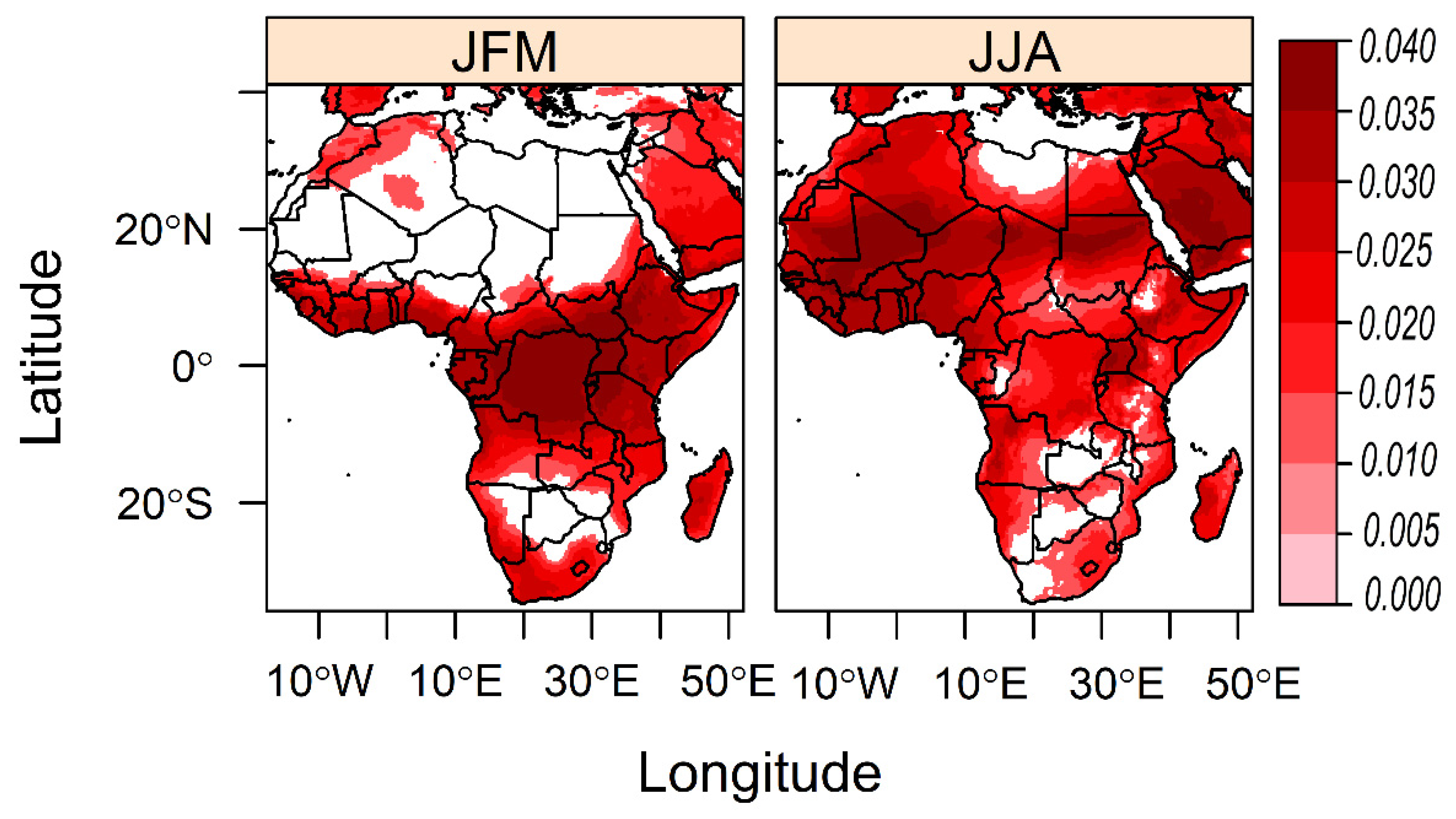
3.1. Trend Analysis of the Atmospheric Layer Thickness

Figure 2 shows the seasonal trend in the atmospheric height between 850 and 1000 hPa. The trend analysis is based on the z-score standardized seasonal mean values derived from ERA5 data. By standardizing these seasonal mean values, we enable spatial comparison of trends, accounting for each location’s historical variability. Thus, the trend values derived from this standardized data are interpreted in terms of standard deviations, providing a more meaningful understanding of the variations relative to historical norms. For large parts of Africa, the vertical extent between the pressure levels has increased significantly. However, the magnitude of the increase varies spatially and seasonally. During JFM, maximum heating is experienced towards southward regions of the equator and the trend magnitude being largest in the Congo Basin (i.e., between 0° to 10° S). Conversely, during JJA, when the region of maximum heating is more northward of the equator, the trend magnitude is largest in parts of northern and northwestern Africa (about 0° to 23° N). The spatial extent of the positive trend is higher during JJA. During JFM, large parts of the Sahel and the Sahara Desert did not experience statistically significant changes in the thickness layer. Also, in parts of southern Africa, and central/northern Libya, the trends are not significant during both JJA and JFM. The regions with increasing trends are also consistent in the NCEP data (Figure S1).

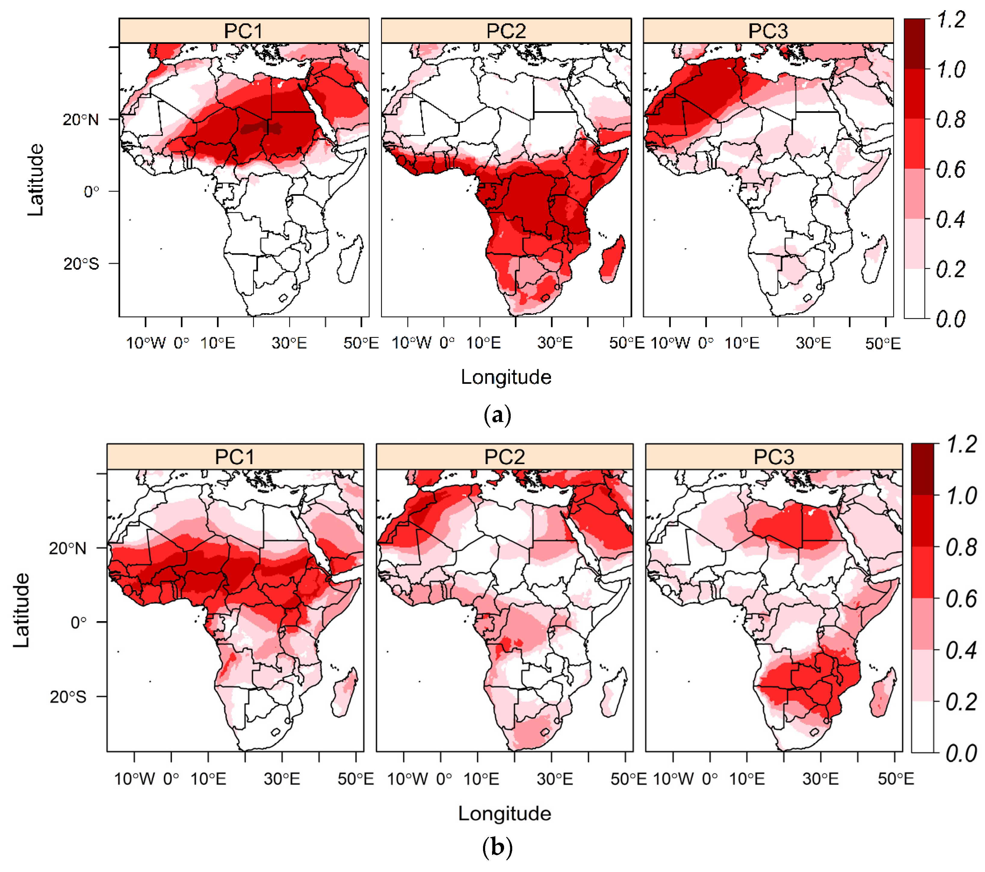
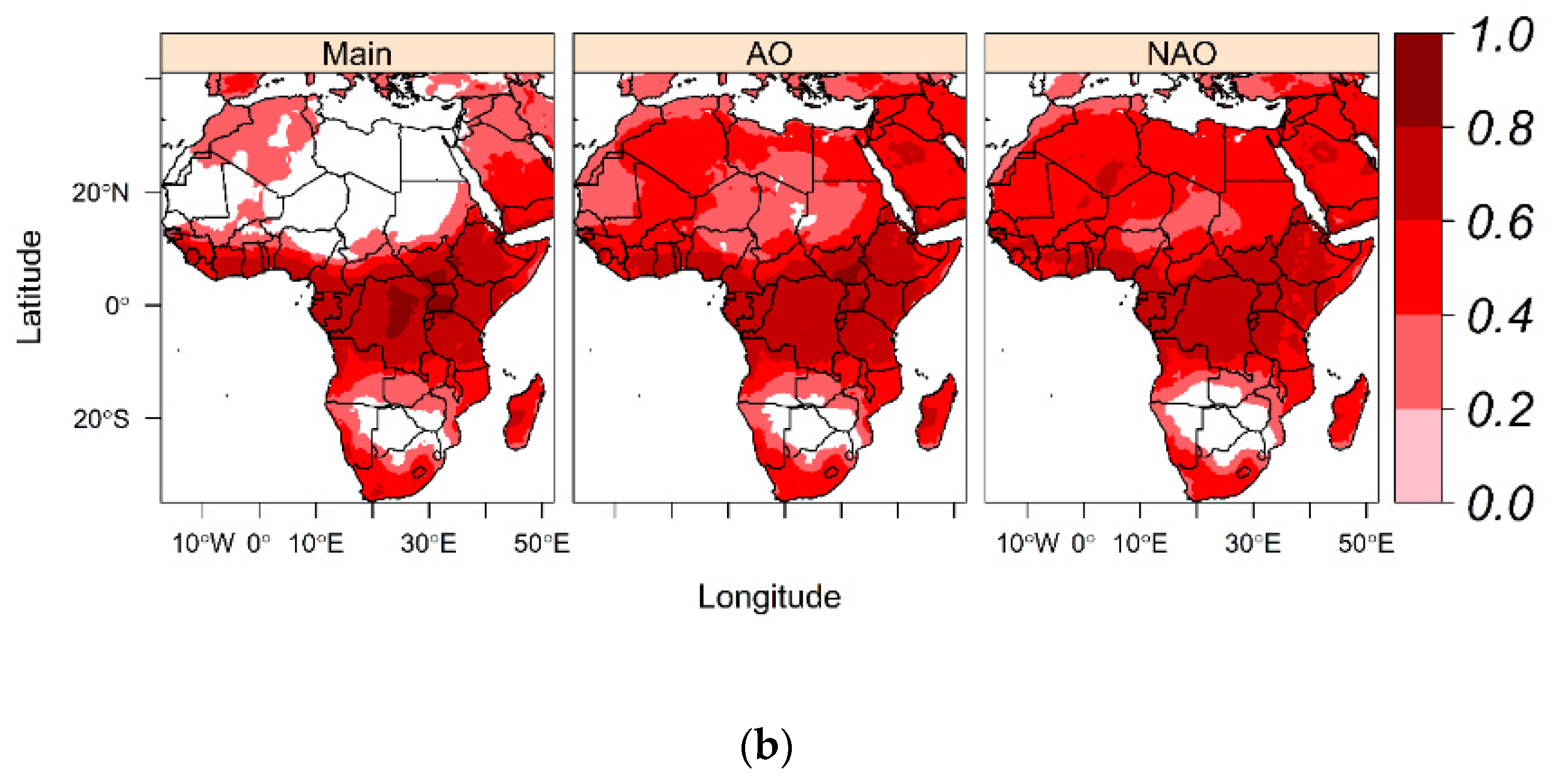
3.2. Seasonal Spatial Decomposition of the Atmospheric Layer Thickness

Given the spatiotemporal variability of the trends (Figure 2), to effectively diagnose the climate signals associated with the increasing trend of the layer thickness over specific regions as well as diagnose a possible explanation of why the thickness layer in large parts of the Sahel and Sahara Desert is not increasing during JFM, the thickness layer during JJA and JFM was spatially decomposed. This resulted in the three optimal variability patterns displayed in Figure 3. The variability patterns in Figure 3 can be interpreted as regions with coherent variability of seasonal thickness. Figures S2–S5 show that enhanced warm air advection (mostly from the Oceans) largely contributes to increase the thickness layers, while enhanced cold air advection contributes to a decrease in the thickness layer.
The spatial decomposition of the thickness layers enables a more focused analysis of the processes associated with thickness variability over a given coherent region in Figure 3. The PC scores were structured such that the positive phase (negative phase) contains an above-average (below-average) atmospheric thickness signal.
From Figure 3a, it shows that during JFM, the northern parts of Africa can be grouped into the northwestern (PC3) and northeastern (PC1) regions, in terms of atmospheric layer thickness between 1000 and 850 hPa. The thickness layer from the central to southern parts of Africa is also coherent, though the magnitude of the coherency weakens over the subtropical parts of southern Africa (i.e., the weak loading magnitude in subtropical southern Africa under PC2, Figure 3a) but is strongest in the Congo Basin. An entirely different spatial structure can be seen during JJA (Figure 3b). First, there is strong coherency of the thickness layer over the Sahel and equatorial parts of North Africa (PC1, Figure 3b). The northwestern region (Morocco, parts of northern Algeria, and Mauritania) is also correlated in terms of JJA atmospheric layer thickness (PC2, Figure 3b). Furthermore, there appears to be some coupling between the northeastern and central parts of southern Africa (PC3, Figure 3b).
It should be noted that during JFM, the Sahel and Sahara Desert were notably characterized by no statistically significant increase in the atmospheric layer thickness (cf. Figure 2). The regions in both PC1 and PC3 both make up the northern domain with no significant trend in thickness layer during JFM (Figure 2 and Figure 3). Both PC1 and PC3 are significantly correlated negatively with the North Atlantic Oscillation (NAO) [38] and the Artic Oscillation (AO) [39] as shown in Table S1. The AO is a pattern of atmospheric pressure anomalies across the polar and mid-latitude regions of the Northern Hemisphere. In its positive phase, the AO shows stronger than usual westerly winds around the Arctic, confining colder air to the polar region. The negative phase features weaker polar winds, allowing colder Arctic air to flow into mid-latitude regions. The NAO, on the other hand, is associated with the difference in atmospheric pressure at sea level between the Icelandic Low and the Azores High. During its positive phase, the NAO is characterized by stronger-than-average westerlies across the North Atlantic, often leading to cooler conditions in parts of North Africa. In the negative phase, this pattern is reversed, potentially resulting in warmer conditions in parts of North Africa. The negative correlation implies that the positive phase of the NAO contributes to a thinner atmospheric layer over the Sahel and Sahara Desert.
Regression analysis and partial correlations were applied to further investigate if the signal of positive NAO and AO are largely contributing to the stable atmosphere over the Sahel and the Sahara Desert. Figure 4a confirms that the NAO and AO are negatively associated with the thickness layer over the northern parts of Africa. Also, when the signal of the NAO and the AO are controlled using partial correlations, a significant increase in the layer height emerges over the Sahel and the Sahara Desert (Figure 4b), which strongly suggests that the AO and the NAO significantly modulate the trends in the thickness layer over the Sahel and the Sahara Desert.
Furthermore, from Tables S1 and S2, during JFM and JJA, the increase in the atmospheric layer thickness over PC2 in each season is significantly and dominantly correlated with the GMLOT (distance correlation = 0.77 during JFM and 0.66 during JJA). This shows the relationship between global warming and the increase in atmospheric layer thickness over the respective regions in PC2.

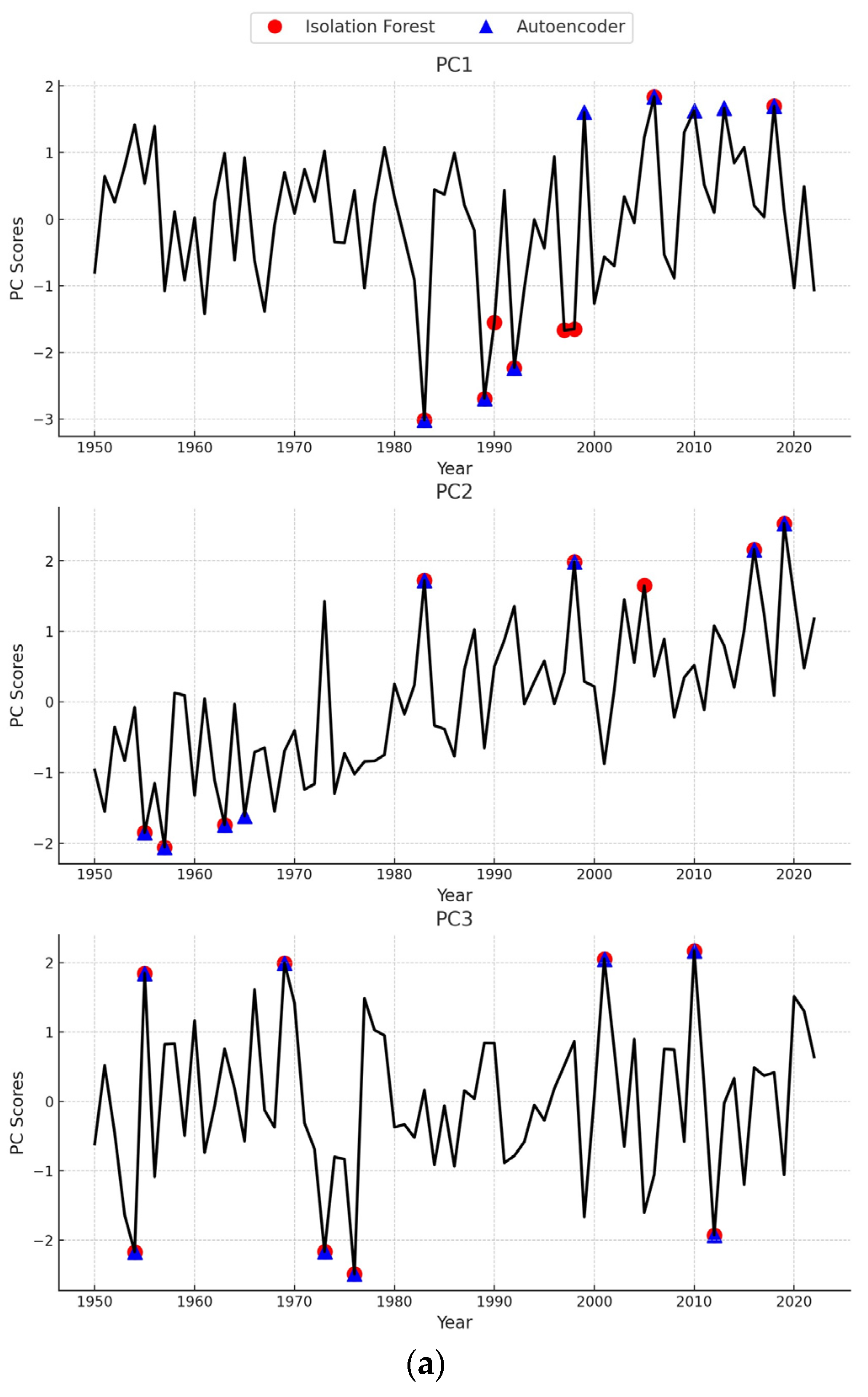
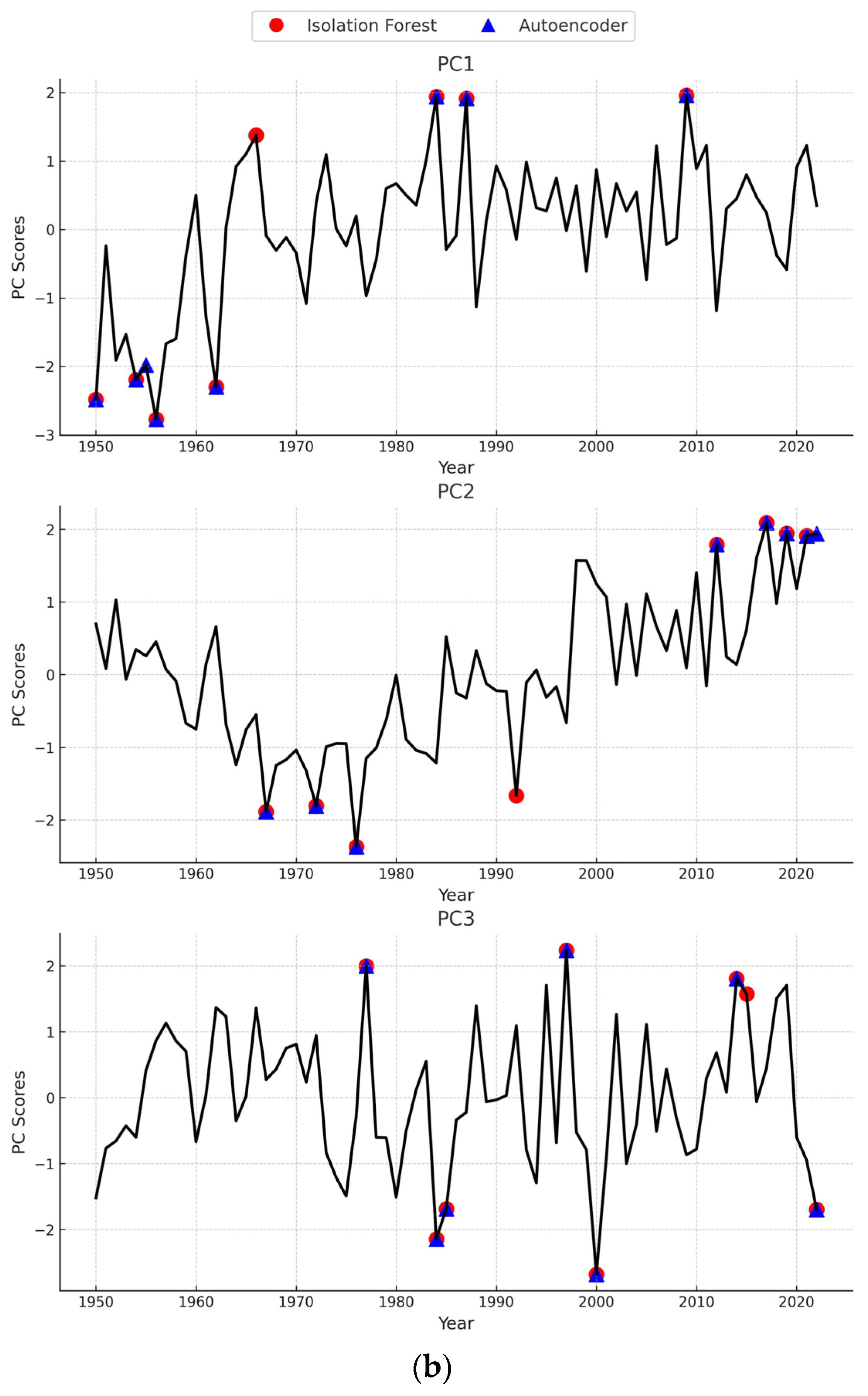
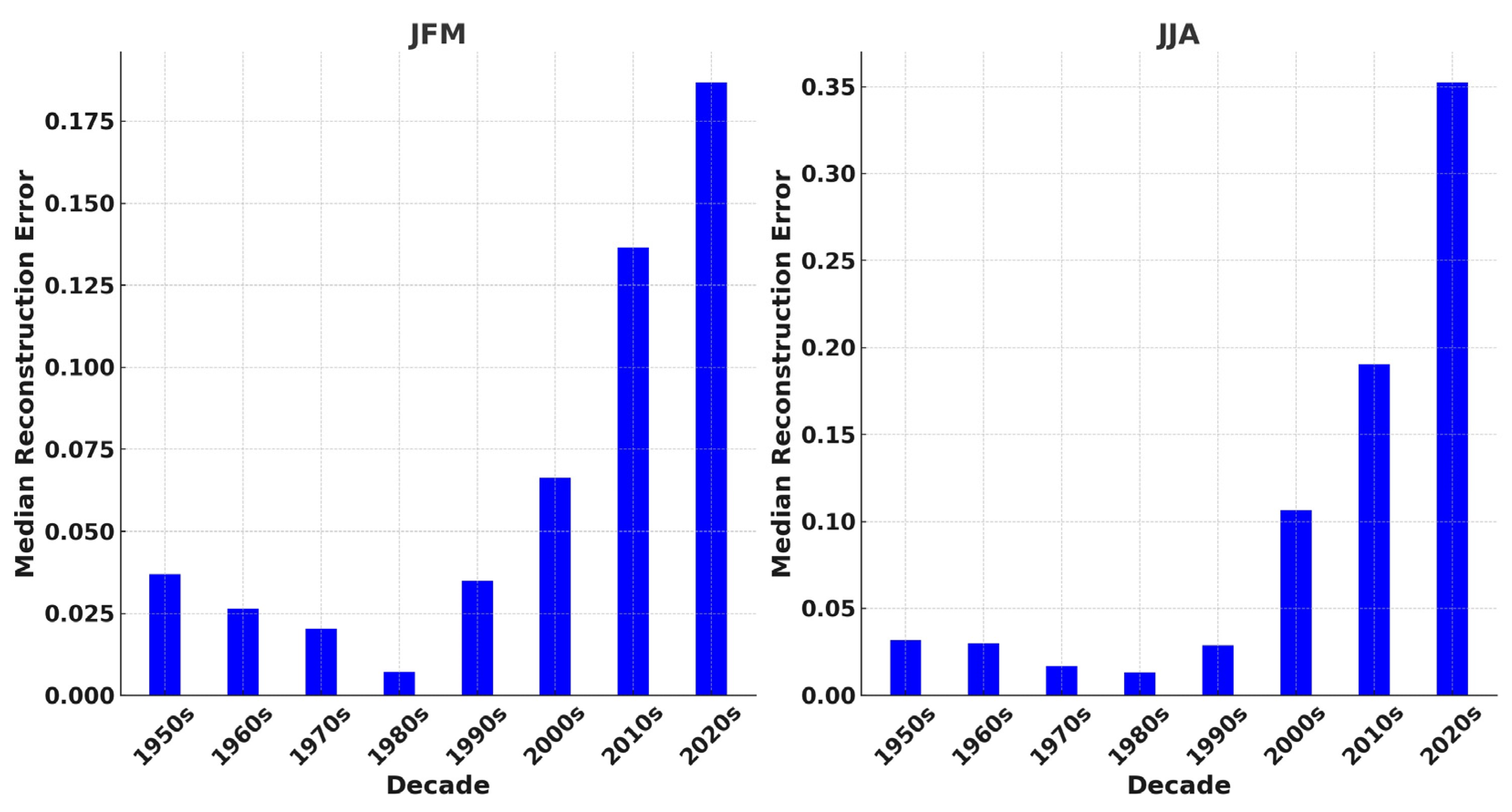
3.3. Application of Deep Learning in Assessing Regional Thickness Changes

This section utilizes the autoencoder artificial neural network to pinpoint years of strong anomalies in the layer thickness, as well as assess the fingerprint of global warming on the regional thickness. Figure 5 shows the time series (PC scores) of the regional spatial patterns in Figure 3. Based on the modified Mann–Kendall test applied at a 95% confidence level, there are significant positive trends under PCs 1 and 2 during JJA (tau statistic = 0.29 and 0.35, respectively) and PC2 during JFM (tau statistic = 0.51). The positive trend implies an increase in the regional thickness layer since positive anomalies of scores are structured to contain above-average thickness signals. The tau statistic indicates that the positive trend is strongest during JFM under PC2, i.e., the southern regions, specifically over the Congo Basin which is the center of action (cf. Figure 3a—based on the loading magnitude).
From Figure 5, the years detected to have strong anomalies are generally consistent with autoencoders and Isolation Forest, which is promising for the reliability of the results. Table S3 shows the years designated to have strong thickness anomalies over each of the homogeneous regions from autoencoders and Isolation Forest for a more detailed evaluation of the consistency of the results from both algorithms.
For all classified regions, Figure 5a indicates that since the 1990s, during JFM, the Congo Basin has experienced anomalous increases in its thickness layer (i.e., PC2 in Figure 5a). Subsequently, assessing the fingerprint of climate change on the two homogeneous regions (that is PC2 during JFM and JJA) that are significantly correlated with GMLOT (Tables S1 and S2), the results (Figure 6) show that the autoencoder model struggled to reconstruct the joint temporal variability of the GMLOT and thickness layer towards the end of the analysis period. This enabled highlighting periods with joint anomalous global warming signals and thickness increases across classified regions in Africa. Figure 7 further supports that since the 2000s, the joint relationship between the global warming signal and thickness increase over parts of Africa has amplified.

4. Discussion

The observed positive trend in the thickness between 1000 and 850 hPa since 1950 raises much concern about the region’s climate system and its sustainability. Our results show that the Congo Basin, a vital component of Africa’s climatic system, is experiencing a significant increase in its thickness layer during the austral summer. These findings, supported by deep autoencoder neural networks, suggest the fingerprint of global warming on the increasing thickness layer in the Congo Basin during austral summer (JFM). The implications of these changes are expected to be multifaceted, affecting temperature, precipitation patterns, and consequently, the region’s unique ecosystem. Moreover, these findings are consistent with other studies that have reported historical and future changes in the climate of the Congo Basin, manifesting as positive temperature trends and increase in rainfall variability [40,41,42,43]
These changes require adaptive strategies in water resource management, agriculture, and conservation to mitigate their impacts and ensure the resilience of the Congo Basin’s environment and communities. Thus, as we move forward, it is imperative to integrate these insights into policy and conservation efforts, to safeguard the Congo Basin’s ecosystem against the adverse effects of global warming and ensure its sustainability for future generations.
The Sahel and the Sahara are regions characterized by distinct and contrasting climates. The Sahel, a semi-arid region, acts as a transition zone between the Sahara Desert to the north and more humid savannas to the south. Its climate is highly variable and sensitive to small shifts in weather patterns [44]. The Sahara, the world’s largest hot desert, has an extremely arid climate with minimal precipitation and high temperatures. Both the Sahel and the Sahara are inherently vulnerable to climatic changes due to their existing extreme conditions [45].
Interestingly, our results indicated that the atmospheric layer thickness is not significantly changing over the Sahel and the Sahara during austral summer. Nonetheless, the thickness layer has a positive trend in austral winter (JJA). A significant factor modulating the climate of the Sahel and the Sahara during austral summer is the NAO—a large-scale atmospheric pressure pattern. During its positive phase, the NAO tends to bring colder conditions to parts of Northern Africa, including the Sahel and the Sahara [46]. This phenomenon is suggested in this study to counteract the effects of increasing atmospheric layer thickness over the Sahel and the Sahara during austral summer when the NAO signal is at its maximum [46].
Finally, in addressing the impact of climate change on Africa’s atmosphere, particularly the increase in atmospheric layer thickness in the Congo Basin and northwestern Africa, our study informs several key policy decisions. These include implementing emission reduction strategies, enforcing deforestation control, investing in climate research, and monitoring and developing water management and resilient agricultural policies. Furthermore, urban planning and infrastructure development must be climate-conscious, and public awareness and education campaigns are essential. International cooperation and policy coordination are also critical in this context. These policies, when integrated and implemented effectively, can significantly mitigate the adverse effects of climate.

5. Conclusions

In this study, we applied advanced machine learning techniques to assess changes in the African partial atmospheric layer. The rotated PCA was utilized to spatially decompose the atmospheric layer thickness allowing for the identification of (homogenous) regions that covaried in terms of seasonal atmospheric layer thickness. A deep autoencoder was further utilized to examine the years with strong anomalies in the thickness over a given homogeneous region as well as to examine the fingerprint of global warming over a given homogenous region. We found that the partial atmospheric layer thickness is changing heterogeneously in space and time. The spatial extent of the increase in the thickness layer is higher in austral winter, with a larger magnitude of increase in parts of the northern/northwestern parts of Africa. In austral summer, the Congo Basin is the hotspot for a thickening atmospheric layer and our neural network models suggest the fingerprint of global warming on this increase. During austral summer, we did not find any significant changes in the thickness layer over the Sahel and the Sahara. These findings underscore the need to monitor the climate of Africa as well as developing sustainable strategies to mitigate the adverse effects of climate variability and change in the region.
The major limitation of this study is the uncertainty associated with the ERA5 reanalysis dataset that provides the best estimate of past climate and weather. Nonetheless, we externally validated our study using the NCEP reanalysis. In future studies, we aim to develop and foster the applications of more advanced machine learning techniques integrated with neural networks to assess historical and future changes in the African climate.

Supplementary Materials

The following supporting information can be downloaded at: https://www.mdpi.com/article/10.3390/su16010256/s1, Figure S1: Trends in atmospheric layer thickness between 850 hPa and 1000 hPa from 1950 to 2022 from NCEP-NCAR reanalysis; Figure S2: Composite anomaly maps of SST and 850 hPa wind vectors associated with below-average thickness layers in the JFM coherent regions in Figure 2b; Figure S3: Composite anomaly maps of SST and 850 hPa wind vectors associated with below-average thickness layers in the JFM coherent regions in Figure 2b; Figure S4: Composite anomaly maps of SST and 850 hPa wind vectors associated with above-average thickness layers in the JFM coherent regions in Figure 2a; Figure S5: Composite anomaly maps of SST and 850 hPa wind vectors associated with above-average thickness layers in the JFM coherent regions in Figure 2b; Table S1: Kendall correlation and distance correlation (that captures non-linear relationships) between the JFM thickness layer variability patterns and climate indices. Table S2: Kendall correlation and distance correlation (that captures non-linear relationships) between the JJA thickness layer variability patterns and climate indices. Table S3: Ten percent of the years with strongest anomalies based on the autoencoder and Isolation Forest Algorithm.

Author Contributions

Conceptualization, C.C.I., I.-O.A., C.N., E.A. and L.B.; methodology, C.C.I., I.-O.A., C.N., E.A. and L.B.; software, C.C.I., I.-O.A., C.N., E.A. and L.B.; validation, C.C.I., I.-O.A., C.N., E.A. and L.B.; formal analysis, C.C.I., I.-O.A., C.N., E.A. and L.B.; investigation, C.C.I., I.-O.A., C.N., E.A. and L.B.; resources, C.C.I., I.-O.A., C.N., E.A. and L.B.; data curation, C.C.I., I.-O.A., C.N., E.A. and L.B.; writing—C.C.I. and I.-O.A.; writing—review and editing, C.C.I., I.-O.A., C.N., E.A. and L.B.; visualization, C.C.I., I.-O.A., C.N., E.A. and L.B.; supervision, C.C.I., I.-O.A., C.N., E.A. and L.B.; project administration, C.C.I., I.-O.A., C.N., E.A. and L.B.; funding acquisition, C.C.I., I.-O.A., C.N., E.A. and L.B. All authors have read and agreed to the published version of the manuscript.

Funding

This research received no external funding. Chibuike Chiedozie Ibebuchi is funded as a Post-doctoral Researcher at Kent State University.

Institutional Review Board Statement

Not applicable.

Informed Consent Statement

Not applicable.

Data Availability Statement

ERA5 data are available at https://cds.climate.copernicus.eu/cdsapp#!/dataset, and NCEP data are available at https://psl.noaa.gov/data/gridded/data.ncep.reanalysis.html. All links accessed on 14 September 2023.

Conflicts of Interest

The authors declare no conflicts of interest.

References

  1. Sylla, M.B.; Nikiema, P.M.; Gibba, P.; Kebe, I.; Klutse, N.A.B. Climate Change over West Africa: Recent Trends and Future Projections. Adapt. Clim. Chang. Var. Rural. West Afr. 2016, 25–40. [Google Scholar] [CrossRef]
  2. Nicholson, S.E. Climate of the Sahel and West Africa. Oxford Res. Encycl. Clim. Sci. 2018. [Google Scholar] [CrossRef]
  3. Kruger, A.C.; Shongwe, S. Temperature trends in South Africa: 1960–2003. Int. J. Clim. 2004, 24, 1929–1945. [Google Scholar] [CrossRef]
  4. MacKellar, N.; New, M.; Jack, C. Observed and modelled trends in rainfall and temperature for South Africa: 1960–2010. S. Afr. J. Sci. 2014, 110, 1–13. [Google Scholar] [CrossRef]
  5. Ceccherini, G.; Russo, S.; Ameztoy, I.; Francesco Marchese, A.; Carmona-Moreno, C. Heat waves in Africa 1981–2015, observations and reanalysis. Nat. Hazards Earth Syst. Sci. 2017, 17, 115–125. [Google Scholar] [CrossRef]
  6. Ibebuchi, C.; Lee, C. Global trends in atmospheric layer thickness since 1940 and relationships with tropical and extratropical climate forcing. Environ. Res. Lett. 2023, 18, 104007. [Google Scholar] [CrossRef]
  7. Kelley, O.A. Where the Least Rainfall Occurs in the Sahara Desert, the TRMM Radar Reveals a Different Pattern of Rainfall Each Season. J. Clim. 2014, 27, 6919–6939. [Google Scholar] [CrossRef]
  8. Dyer, E.L.E.; Jones, D.B.A.; Li, R.; Sawaoka, H.; Mudryk, L. Sahel precipitation and regional teleconnections with the Indian Ocean. J. Geophys. Res. Atmos. 2017, 122, 5654–5676. [Google Scholar] [CrossRef]
  9. Russo, S.E.; Kitajima, K. The Ecophysiology of Leaf Lifespan in Tropical Forests: Adaptive and Plastic Responses to Environmental Heterogeneity. Trop. Tree Physiol. Adapt. Responses A Change Environ. 2016, 357–383. [Google Scholar] [CrossRef]
  10. Dosio, A.; Fischer, E.M. Will Half a Degree Make a Difference? Robust Projections of Indices of Mean and Extreme Climate in Europe Under 1.5 °C, 2 °C, and 3 °C Global Warming. Geophys. Res. Lett. 2018, 45, 935–944. [Google Scholar] [CrossRef]
  11. Ayugi, B.; Shilenje, Z.W.; Babaousmail, H.; Lim Kam Sian, K.T.C.; Mumo, R.; Dike, V.N.; Iyakaremye, V.; Chehbouni, A.; Ongoma, V. Projected changes in meteorological drought over East Africa inferred from bias-adjusted CMIP6 models. Nat. Hazards 2022, 113, 1151–1176. [Google Scholar] [CrossRef] [PubMed]
  12. Ghansah, B.; Nyamekye, C.; Owusu, S.; Agyapong, E. Mapping flood prone and Hazards Areas in rural landscape using landsat images and random forest classification: Case study of Nasia watershed in Ghana. Cogent Eng. 2021, 8, 1923384. [Google Scholar] [CrossRef]
  13. Engelbrecht, F.; Adegoke, J.; Bopape, M.-J.; Naidoo, M.; Garland, R.; Thatcher, M.; McGregor, J.; Katzfey, J.; Werner, M.; Ichoku, C.; et al. Projections of rapidly rising surface temperatures over Africa under low mitigation. Environ. Res. Lett. 2015, 10, 085004. [Google Scholar] [CrossRef]
  14. Dosio, A. Projection of temperature and heat waves for Africa with an ensemble of CORDEX Regional Climate Models. Clim. Dyn. 2017, 49, 493–519. [Google Scholar] [CrossRef]
  15. James, R.; Washington, R. Changes in African temperature and precipitation associated with degrees of global warming. Clim. Change 2013, 117, 859–872. [Google Scholar] [CrossRef]
  16. White, D.; Richman, M.; Yarnal, B. Climate regionalization and rotation of principal components. Int. J. Clim. 1991, 11, 1–25. [Google Scholar] [CrossRef]
  17. Cheng, S.; Prentice, I.C.; Huang, Y.; Jin, Y.; Guo, Y.-K.; Arcucci, R. Data-driven surrogate model with latent data assimilation: Application to wildfire forecasting. J. Comput. Phys. 2022, 464, 111302. [Google Scholar] [CrossRef]
  18. Tibau, X.A.; Reimers, C.; Requena-Mesa, C.; Runge, J. Spatio-Temporal Autoencoders in Weather and Climate Research. Deep. Learn. Earth Sci. A Compr. Approach Remote Sens. Clim. Sci. Geosci. 2021, 186–203. [Google Scholar] [CrossRef]
  19. Rautela, K.S.; Singh, S.; Goyal, M.K. Characterizing the spatio-temporal distribution, detection, and prediction of aerosol atmospheric rivers on a global scale. J. Environ. Manag. 2024, 351, 119675. [Google Scholar] [CrossRef]
  20. Meghani, S.; Singh, S.; Kumar, N.; Goyal, M.K. Predicting the spatiotemporal characteristics of atmospheric rivers: A novel data-driven approach. Glob. Planet. Chang. 2023, 231, 104295. [Google Scholar] [CrossRef]
  21. Donnelly, J.; Daneshkhah, A.; Abolfathi, S. Forecasting global climate drivers using Gaussian processes and convolutional autoencoders. Eng. Appl. Artif. Intell. 2024, 128, 107536. [Google Scholar] [CrossRef]
  22. Hersbach, H.; Bell, B.; Berrisford, P.; Hirahara, S.; Horányi, A.; Muñoz-Sabater, J.; Nicolas, J.; Peubey, C.; Radu, R.; Schepers, D.; et al. The ERA5 global reanalysis. Q. J. R. Meteorol. Soc. 2020, 146, 1999–2049. [Google Scholar] [CrossRef]
  23. Kalnay, E.; Kanamitsu, M.; Kistler, R.; Collins, W.; Deaven, D.; Gandin, L.; Iredell, M.; Saha, S.; White, G.; Woollen, J.; et al. The NCEP/NCAR 40-Year Reanalysis Project. Bull. Am. Meteorol. Soc. 1996, 77, 437–471. [Google Scholar] [CrossRef]
  24. Mocsari, E.; Stone, S.S. Colostral IgA, IgG, and IgM-IgA Fractions as Fluorescent Antibody for the Detection of the Coronavirus of Transmissible Gastroenteritis. Am. J. Vet. Res. 1978, 39, 1442–1446. [Google Scholar] [PubMed]
  25. Yue, S.; Wang, C.Y. The Mann-Kendall Test Modified by Effective Sample Size to Detect Trend in Serially Correlated Hydrological Series. Water Resour. Manag. 2004, 18, 201–218. [Google Scholar] [CrossRef]
  26. Benjamini, Y. Discovering the False Discovery Rate. J. R. Stat. Soc. Ser. B Stat. Methodol. 2010, 72, 405–416. [Google Scholar] [CrossRef]
  27. Ibebuchi, C.C.; Abu, I.-O. Rainfall variability patterns in Nigeria during the rainy season. Sci. Rep. 2023, 13, 7888. [Google Scholar] [CrossRef] [PubMed]
  28. Ibebuchi, C.; Richman, M.; Chiedozie Ibebuchi, C.; Richman, M.B. Circulation typing with fuzzy rotated T-mode principal component analysis: Methodological considerations. Theor. Appl. Clim. 2023, 153, 495–523. [Google Scholar] [CrossRef]
  29. R Core Team. R: A Language and Environment for Statistical Computing; R Foundation for Statistical Computing: Vienna, Austria, 2022. [Google Scholar]
  30. Hinton, G.E.; Salakhutdinov, R.R. Reducing the Dimensionality of Data with Neural Networks. Science 2006, 313, 504–507. [Google Scholar] [CrossRef]
  31. Zhou, C.; Paffenroth, R.C. Anomaly Detection with Robust Deep Autoencoders. In Proceedings of the 23rd ACM SIGKDD International Conference on Knowledge Discovery and Data Mining, Halifax, NS, Canada, 13–17 August 2017; Part F129685. pp. 665–674. [Google Scholar]
  32. Chen, Z.; Yeo, C.K.; Lee, B.S.; Lau, C.T. Autoencoder-Based Network Anomaly Detection. In Proceedings of the 2018 Wireless Telecommunications Symposium (WTS), Phoenix, AZ, USA, 17–20 April 2018. [Google Scholar] [CrossRef]
  33. Homayouni, H.; Ghosh, S.; Ray, I.; Gondalia, S.; Duggan, J.; Kahn, M.G. An Autocorrelation-Based LSTM-Autoencoder for Anomaly Detection on Time-Series Data. In Proceedings of the 2020 IEEE International Conference on Big Data (Big Data), Atlanta, GA, USA, 10–13 December 2020; pp. 5068–5077. [Google Scholar] [CrossRef]
  34. Mendes, T.; Cardoso, P.J.S.; Monteiro, J.; Raposo, J. Anomaly Detection of Consumption in Hotel Units: A Case Study Comparing Isolation Forest and Variational Autoencoder Algorithms. Appl. Sci. 2022, 13, 314. [Google Scholar] [CrossRef]
  35. Edelmann, D.; Móri, T.F.; Székely, G.J. On relationships between the Pearson and the distance correlation coefficients. Stat. Probab. Lett. 2021, 169, 108960. [Google Scholar] [CrossRef]
  36. Goodfellow, I. NIPS 2016 Tutorial: Generative Adversarial Networks. arXiv 2016, arXiv:1701.00160. [Google Scholar]
  37. Kingma, D.P.; Rezende, D.J.; Mohamed, S.; Welling, M. Semi-Supervised Learning with Deep Generative Models. Adv. Neural Inf. Process. Syst. 2014, 4, 3581–3589. [Google Scholar]
  38. Hurrell, J.W.; Kushnir, Y.; Ottersen, G.; Visbeck, M. An overview of the North Atlantic Oscillation. Geophys. Monogr. Ser. 2003, 134, 1–35. [Google Scholar] [CrossRef]
  39. Wang, J.; Ikeda, M. Arctic oscillation and Arctic sea-ice oscillation. Geophys. Res. Lett. 2000, 27, 1287–1290. [Google Scholar] [CrossRef]
  40. Wilkie, D.; Morelli, G.; Rotberg, F.; Shaw, E. Wetter isn’t better: Global warming and food security in the Congo Basin. Glob. Environ. Change 1999, 9, 323–328. [Google Scholar] [CrossRef]
  41. Haensler, A.; Saeed, F.; Jacob, D. Assessing the robustness of projected precipitation changes over central Africa on the basis of a multitude of global and regional climate projections. Clim. Chang. 2013, 121, 349–363. [Google Scholar] [CrossRef]
  42. Samba, G.; Nganga, D. Minimum and Maximum Temperature Trends in Congo-Brazzaville: 1932–2010. Atmos. Clim. Sci. 2014, 4, 404–430. [Google Scholar] [CrossRef]
  43. Creese, A.; Washington, R.; Jones, R. Climate change in the Congo Basin: Processes related to wetting in the December–February dry season. Clim. Dyn. 2019, 53, 3583–3602. [Google Scholar] [CrossRef]
  44. Zakari, S.; Ibro, G.; Moussa, B.; Abdoulaye, T. Adaptation Strategies to Climate Change and Impacts on Household Income and Food Security: Evidence from Sahelian Region of Niger. Sustainability 2022, 14, 2847. [Google Scholar] [CrossRef]
  45. Tian, C.; Huang, G.; Lu, C.; Song, T.; Wu, Y.; Duan, R. Northward Shifts of the Sahara Desert in Response to Twenty-First-Century Climate Change. J. Clim. 2023, 36, 3417–3435. [Google Scholar] [CrossRef]
  46. Zhou, L.; Hua, W.; Nicholson, S.E.; Clark, J.P. Interannual teleconnections in the Sahara temperatures associated with the North Atlantic Oscillation (NAO) during boreal winter. Clim. Dyn. 2023, 1–21. [Google Scholar] [CrossRef]
Figure 1. Flow chart of the methods utilized in assessing spatiotemporal changes in Africa’s atmospheric layer thickness.
Sustainability 16 00256 g001
Figure 2. Seasonal trend in atmospheric thickness between the 1000 and 850 hPa pressure levels from 1950 to 2022. Only those grid points exhibiting a statistically significant trend at a 95% confidence level are shaded. The trend analysis is based on the z-score standardized seasonal mean values from ERA5 data. The trend values derived from this standardized data are interpreted in terms of standard deviations.
Sustainability 16 00256 g002
Figure 3. Spatial decomposition of the thickness layer during JFM (a) and JJA (b) using rotated S-mode PCA. The color is the rotated PC loadings. The analysis period is from 1950 to 2022.
Sustainability 16 00256 g003
Figure 4. Regression of the AO and the NAO index onto the JFM thickness layer between 850 hPa and 1000 hPa (a), and (partial) correlation between the thickness layer and time (“Main”), and with the signal of the AO and the NAO controlled for the time changes in the thickness layer (b). The analysis period is from 1950 to 2022. Regression coefficients in (b) are in the units of m/year. Only statistically significant values at a 95% confidence level are plotted.
Sustainability 16 00256 g004aSustainability 16 00256 g004b
Figure 5. Time series (PC scores) of the spatial variability patterns in Figure 3 from 1950 to 2022 during JFM (a) and JJA (b). Positive (negative) anomalies were structured to represent periods is above-average (below-average) thickness anomaly. Markers indicate 10% of years with strong anomalies in the regional layer thickness based on the autoencoder and Isolation Forest algorithms.
Sustainability 16 00256 g005aSustainability 16 00256 g005b
Figure 6. Reconstruction errors from the autoencoder model (1950 to 2022) for PC2 that are significantly related to the global warming signal during JFM and JJA. The input is from GMLOT and the PC scores from PC2 during JFM and JJA.
Sustainability 16 00256 g006
Figure 7. Median value of the reconstruction error per decade for the time series in Figure 6 during JFM and JJA. The input in the autoencoder model is GMLOT and the PC scores of PC2.
Sustainability 16 00256 g007
Disclaimer/Publisher’s Note: The statements, opinions and data contained in all publications are solely those of the individual author(s) and contributor(s) and not of MDPI and/or the editor(s). MDPI and/or the editor(s) disclaim responsibility for any injury to people or property resulting from any ideas, methods, instructions or products referred to in the content.

