Abstract
Carbon trading markets are crucial policy instruments in carbon emission reduction and carbon neutrality. Yet, China’s pilot programs encounter diverse operational modes and environmental factors that might impact their effectiveness. This study uses panel data from 30 provinces (2000–2019) in China and the regression control method to evaluate and analyze the heterogeneous effects of carbon trading pilots (CTPs) on emission reduction. Results reveal three types of CTP effects which are as follows: reducing both total carbon emissions (TCEs) and carbon intensity (CI) as noticed in Shanghai; decreasing CI while increasing TCE as seen in Beijing, Tianjin, Guangdong, and Hubei; and raising both TCE and CI as observed in Chongqing and Fujian. Significantly, market mechanisms in carbon pricing and state intervention, including of state-owned enterprises, play notable roles in these effects. Furthermore, CTP policies display both intensity reduction and energy rebound effects; the direction of carbon emission reduction relies on the balance between these effects. The findings offer empirical support to enhance carbon market effectiveness and provide valuable insights for regions in China and globally in order to tailor policies based on their specific conditions.
1. Introduction
Since China’s reform and opening up, its economy has grown remarkably. This growth has led to a surge in fossil energy demand due to rapid industrialization and urbanization, causing a substantial increase in carbon dioxide emissions []. China has now become one of the world’s top contributors to carbon emissions []. According to World Bank data, China’s share of global carbon emissions rose from 13.78% to 32.61% between 2000 and 2020. Despite significant pressure to reduce emissions, China, as the largest developing country, makes sustained efforts toward carbon emission reduction and gradually implements plans for carbon peak action as part of the mitigation of global climate change.
In 2011, Carbon trading was initiated in China as part of its energy transition strategy, which aimed to achieve “dual carbon” goals through a comprehensive policy framework. Starting in 2013, seven provincial-level carbon trading pilots (CTPs) were introduced in Shenzhen, Shanghai, Beijing, Guangdong, Tianjin, Hubei, and Chongqing, using market-oriented mechanisms to allocate quotas and restrict emissions from high-carbon industries. However, the pilots differ in their industry focus and quota allocation methods and the carbon prices may change alongside energy prices, etc. []. For instance, the electric power industry is included in Beijing, while in Shanghai, Tianjin, Chongqing, and Hubei, target emissions in sectors like steel and chemicals are included. Meanwhile, Guangdong, Shenzhen, and Hubei adopt auction bidding instead of administrative quotas. Do these variations affect the carbon market’s ability to reduce emissions? Are there differences in emission reduction among these pilots? This paper will provide an analytical framework for addressing these questions.
Maximizing the effectiveness of China’s carbon market is crucial to supporting the achievement of the “dual carbon” goals. Despite having a limited number of pilot regions, China’s carbon emissions, which are covered in this phase, are second only to the European Union’s carbon trading system. These pilot regions span the eastern, central, and western areas of China; each of them features unique characteristics in carbon markets, such as pricing, liquidity, and trading volume. These traits may influence the effectiveness of emission reduction, leading to varied effects of carbon trading pilots (CTPs) on carbon emissions. For instance, considering carbon pricing, the CTP policy impacts carbon emissions and economic growth differently based on distinct carbon price scenarios []. Moreover, variations in industries and enterprises across pilot regions result in differences in the effectiveness of carbon reduction due to varying levels of administrative intervention.
Since the inception of China’s carbon market, scholars have extensively analyzed and demonstrated its effective contribution to emission reduction. Existing research focuses on the average treatment effect (ATE) across all pilots but ignores potential differences in treatment effects among pilots. Solely assessing average treatment effects might overlook the heterogeneous effects of China’s carbon market on carbon emissions, causing biased conclusions and policy inefficiency. Therefore, this study applies the regression control method (RCM) to evaluate heterogeneous carbon emission reduction effects using carbon market data from 30 provinces in China from 2000 to 2019. Additionally, it analyzes influencing factors based on a panel data model. This research holds significant reference value for accurately assessing carbon market effectiveness and achieving emission reduction goals.
Our key academic contributions can be summarized as follows: Firstly, this paper evaluates the diverse carbon emission reduction effects of the CTP policy. Compared with previous studies, we assume that the heterogenous effect exists across multiple pilot regions rather than the uniform effect. To verify our hypothesis, we use the regression control method to assess policy effects individually. Secondly, referring to Rubin’s causal inference framework, we address potential endogeneity concerns in causal inference. We not only undertake controls for policy spillover effects from geographic proximity but also manage interference from provincial-level pairings in aid programs, ensuring more robust policy evaluation results. Lastly, in contrast to prior research, this paper underscores the impact of market operational mechanisms on carbon market effectiveness and demonstrates the significant influence of government intervention levels along with environmental disparities faced by the carbon market. These conclusions provide valuable policy references for countries seeking to further advance and refine their carbon markets in the future.
2. Literature Review and Research Hypothesis
2.1. Research Progress on the Effects of CTP Policy
As carbon markets emerge globally, research on carbon emission trading pilot policies has expanded. Scholars primarily focus on assessing the policies’ efficiency in energy conservation, emission reduction, and productivity enhancement. Chen and Lin (2021) [] observed significant improvements in both total factor carbon performance and energy-carbon performance indexes post-CTP policy implementation measured via global DEA. Zhou and Qi (2022) [] highlighted the CTP’s substantial impact on boosting green total factor energy efficiency through enhancing enterprise technological innovation. Additionally, Hong et al. (2022) [] identified remarkable advancements in city energy efficiency, attributing these to the CTP’s emphasis on green innovation and resource allocation. Furthermore, Yu et al. (2022) [] validated the presence of a green innovation effect resulting from the CTP policy in China.
However, according to Xiao et al. (2023) [], it was demonstrated that the CTP policy did not effectively enhance green total factor productivity within the pilot areas. Similarly, Chen et al. (2021) [] showed that the CTP policy has significantly decreased the proportion of green patents by approximately 9.26% in the current carbon trading market of China. Furthermore, Huang and Chen (2022) [] made up for the neglect of the spatial effect of the CTP policy in previous studies and found that China’s CTP significantly improved the green total factor productivity of pilot cities but produced a negative spatial siphon effect that restricted the growth of green total factor productivity in surrounding cities. Although CTPs can indeed lead to substantial improvements in both single factor energy efficiency and total factor energy efficiency, it was observed that the energy rebound effect in the pilot provinces was notably higher than that in the non-pilot provinces, weakening the energy conservation effect of the CTP [].
From the perspective of mechanistic analysis, some findings revealed that CTPs can stimulate technological progress, factor accumulation, scale allocation, and energy substitution effects, contributing not only to economic growth but also to achieving carbon reduction targets []. In addition, CTPs induce technological innovation effects, energy substitution, and structural upgrading effects; therefore, they enable the realization of green innovation potential []. Tao and Goh (2023) [] demonstrated the mediating effects of total energy consumption, energy consumption structure, and industrial structure upgrades in the incentivizing role of CTPs on carbon emission intensity reduction. In light of China’s CTP policy, Pan et al. (2022) [] highlighted the important moderating roles of government participation and high carbon trading market efficiency on an enterprise’s TFP.
2.2. CTP’s Carbon Emission Reduction Effects and Hypothesis Development
Among numerous emission reduction policies, carbon trading has emerged as an effective strategy to drive green technological innovation and achieve cost-effective carbon reductions on a larger economic scale. This policy primarily utilizes carbon markets for resource allocation and price discovery to achieve emission reductions. Consequently, accurately measuring the carbon reduction effects of this policy has become a focal point for scholars. Previous studies often employ policy evaluation methods for analysis. Yang et al. (2023) [] discovered that the China carbon trading program has significantly reduced China’s carbon emissions by 6.21%. From a comprehensive perspective on carbon sources and sinks, Xia et al. (2021) [] found that CTP policies have made a substantial impact that resulted in at least four million tons of carbon emission reductions per year in the pilot areas during the study period. Furthermore, Xuan et al. (2020) [] assessed the influence of CTP on carbon emission intensity and obtained results similar to those mentioned. Other scholars also verified that regional carbon emissions and carbon emission intensity have both been significantly reduced by the CTP policy [].
Nevertheless, some other scholars have come across more intricate conclusions. In terms of national level carbon emission reduction rates, Zhang et al. (2020) [] found that those pilots demonstrate a faster (slower) rate of carbon emission reductions (or increases) in decoupled (non-decoupled) countries in comparison with countries that have not implemented the CTP. From the perspective of the spatial area, Lan et al. (2020) [] discovered that the CTP has a statistically significant mitigating effect on carbon emissions, with the impact gradually declining from the eastern to the central and, finally, to the western regions. Yi et al. (2020) [] revealed that the implementation of carbon markets in Beijing, Shanghai, and Hubei exhibited a significant inhibitory effect on local carbon emissions while having a promoting effect in Guangdong. However, no significant effect was found in Tianjin. Scholars primarily provide macro-level empirical evidence, yielding mixed conclusions. The research on the micro-level analysis of China’s CTP also showed that the CTP has a tangible impact that is more significant for small-scale firms, non-state-owned firms, and pilot regions with ex-post allowance allocation systems [].
Furthermore, some studies have noticed spatial spillover effects of CTPs. Li and Wang (2022) [] concluded carbon emissions in neighboring regions of pilots were also reduced. Liu et al. (2022) [] found that the CTP policy spillover effect stimulated green innovation in neighboring provinces through innovative growth poles. However, some studies investigated how CTPs can be a threat through the promotion of carbon emissions in the surrounding areas [,].
Therefore, the paper proposes the hypothesis as follows:
H1.
The effects of carbon emission trading pilot policies vary across different pilot regions, warranting an analysis of heterogeneous policy effects.
Compared with European countries and America, China’s carbon market features lower carbon prices and poor liquidity. These might lead to variations in policy effects across different pilots. The characteristics of China’s carbon market are distinct from those in Europe and the United States and are characterized by low carbon prices and poor liquidity. Wang et al. (2022) [] indicated that the efficient market hypothesis does not hold weight in China’s carbon emissions trading market except for Shanghai, which is explained by irrational behaviors, poor information transparency, imperfect market mechanisms, and transaction costs. In addition, the intensity of government intervention also affects the effectiveness of the carbon market. Lin and Huang (2022) [] further showed that the positive carbon emission reduction effect of CTPs was achieved through government intervention rather than market mechanisms.
Based on the analysis above, the paper proposes the second hypothesis as follows:
H2.
The carbon price, liquidity, trading volume, and government intervention within the carbon market could be reasons for the differentiation in policy effects across pilots.
3. Empirical Research Design
The purpose of this part revolves around the two aspects of estimating the carbon emission reduction effects of each pilot and exploring the causal factors of differentiation in pilot effects. Hence, the empirical design comprises the two components of effect evaluation and factor analysis. Concerning effect evaluation, this paper adopts the classic Rubin potential outcome framework to infer causality. The Rubin causal framework sets two states within the carbon trading pilot areas that are the factual outcome and the counterfactual outcome. The factual outcome represents the actual carbon emission growth rate in the carbon trading pilot areas after implementation, while the counterfactual outcome denotes the potential carbon emission growth rate if these areas did not participate in the pilot. According to the Rubin causal framework, the carbon emission reduction effect of carbon trading pilot policies is represented by the difference between actual and potential carbon emission growth rates. However, due to the observability constraint where only actual carbon emission growth rates are measurable, the potential carbon emission growth rate remains unobservable. Therefore, the primary focus of evaluating pilot effects is estimating the potential carbon emission growth rate.
Since 2013, China has gradually introduced carbon trading in seven provincial-level regions and established carbon trading pilot programs. The carbon market was launched in the following regions on the specified dates of November 2013 (Beijing), December 2013 (Tianjin, Shanghai, Guangdong), April 2014 (Hubei), June 2014 (Chongqing), and December 2016 (Fujian). Consequently, the cutoff point was set in 2017 for Fujian, while for the other six regions, it was set in 2014. We will take the seven pilots above as the evaluation subjects for the effects of CTPs.
3.1. Model Specification
Assume that represents the carbon trading pilot area, with the initiation of the pilot at that time as T0 + 1, while other areas not in the pilot are represented by . Following the Rubin potential outcome framework, and are used to, respectively, denote the actual carbon emission growth rate and the potential carbon emission growth rate for the pilot area. In contrast, represents the actual carbon emission growth rates for non-pilot areas for . Suppose is generated by a function of , observed variables , and common factors across individuals,
where is a vector of constants, the loading coefficient denotes the r × 1 vector of constants that may vary across , denotes the fixed individual-specific effects, and is the idiosyncratic error with .
Then, the carbon emission reduction effect of the CTP can be represented as follows:
Since is unobservable, it needs to be estimated. We use the carbon emissions of non-CTP provinces to evaluate . Following the regression control method (RCM) of Hsiao et al. (2012) [] and Hsiao and Zhou (2019) [], we exploit the dependence structure of carbon emissions among provinces. The RCM attributes the cross-dependence to the presence of unobserved common factors that drive the carbon emissions growth of relevant provinces. Under certain conditions, the RCM demonstrates that can be consistently estimated through , where is a subset of and represent the corresponding coefficients. Essentially, estimating is a predictive issue as our primary concern is how closely it aligns with the actual values rather than whether the coefficients are consistently estimated. However, the aforementioned estimation still needs to meet two conditions. The first one is relevance, indicating that both pilot and non-pilot areas are influenced by the same common factors and ensuring the estimation ability. The second one is exogeneity, signifying that non-pilot areas are not affected by the CTP policy in pilots and thereby avoiding endogeneity issues in policy effect evaluation.
Figure 1 depicts the entire process of the RCM. Among these, available methods for step 2 include the best subset, LASSO, forward stepwise as well as backward stepwise regression, while available selection criteria include AICC, AIC, BIC, MBIC, and CV (cross-validation). Available methods for step 3 and step 4 include OLS and LASSO.
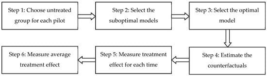
Figure 1.
The flowchart of the RCM.
Referring to existing research, we use LASSO and CV for step 2 and OLS for step 3 and step 4 as benchmarks; we use other combinations for robustness analysis.
Therefore, we can predict the effect of (step 5) due to the implementation of the CTP policy on the CTP province at the time using
Then, the average treatment effect (ATE) can consistently be estimated (step 6) by
Then, we construct the following panel data model to analyze the potential factors contributing to the heterogeneous treatment effects:
Here, represents the policy effect of the -th pilot area at the time . is a column vector consisting of influencing factors and is the corresponding coefficient column vector while and , respectively, denote the regional effect and the error term.
3.2. Variables
3.2.1. Dependent Variables
Due to the promotion of carbon reduction on the carbon market, we selected total carbon emissions (tce) as the first dependent variable. Additionally, China has consistently committed itself to the international community by emphasizing the control of carbon intensity for reducing carbon emissions. Therefore, carbon intensity (ci) is included as another dependent variable for evaluating the effects of CTPs on carbon emissions. Because two dependent variables are log-transformed (lntce and lnci), the difference in the logarithms of variables reflects the change in the growth rate of that variable. The regional gross domestic product (GDP) used to calculate carbon intensity is based on the real regional GDP calculated at constant prices in 1992.
3.2.2. Independent Variables
There are strong correlations between carbon emission variables and economic development. Therefore, we include several independent variables in the model to improve the accuracy of counterfactual predictions. The explanatory variables selected for this study are mainly as follows: 1. The GDP of provincial-level regions, specifically measured as the natural logarithm of the real per capita GDP (lngdppc) and its squared term (lngdppc2), that reflects the inverse U-shaped relationship between economic growth and carbon emissions (namely the EKC hypothesis) calculated at constant prices from 1992. 2. Industrial structures, specifically represented through the share of the secondary industry (indsh) and the share of the service industry (sersh), that reflects whether the change in industrial structure reduces carbon emissions. 3. Economic structure, specifically denoted through the ratio of personal consumption to the regional GDP (ecost), that reflects the share of consumption-based carbon emissions. Due to the lack of personal consumption data, we used consumer goods’ social retail sales as a proxy variable for personal consumption according to existing research. 4. The degree of openness, represented through the ratios of foreign direct investment and total import–export trade volume to the regional GDP (fdide and trade), that reflects the impacts of international capital and trade on carbon emissions. 5. Population agglomeration, measured via the natural logarithm of the year-end resident population size (lnpop), that reflects the scale effect of population on carbon emissions. 6. Fiscal dependency, specifically denoted as the ratio of local general public fiscal revenue to regional GDP (fisde), that reflects the impact of government intervention on enterprise carbon emissions. 7. Innovation activities, expressed as the logarithm of the number of granted patents for effective inventions (lnpaq), that reflects the impact of corporate technological innovation on carbon emissions. 8. Regional energy conservation and emission reduction targets, measured through interaction in terms of that between energy conservation and emission reduction targets of each provincial-level region during the “fifteenth five-year”, “eleventh five-year”, “twelfth five-year”, and “thirteenth five-year” periods and their respective years (plan 2, plan 3, plan 4, plan 5), that reflect the impact of government targets on enterprise carbon emissions.
3.2.3. Mechanism and Environmental Variables
To analyze the reasons behind the differentiation in the impact of the CTP policy, we dissect the carbon market situations in the seven pilot regions from the two perspectives of market mechanisms and administrative interventions.
In terms of market mechanisms, we evaluate carbon market transactions based on the three key aspects of carbon trading prices, carbon market liquidity, and carbon trading volume. To elaborate, carbon trading prices are determined through calculating the annual average of daily closing prices (price). Carbon market liquidity is gauged by the percentage of days with non-zero transactions (liqui); carbon trading volume is computed as the annual trading volume relative to the region’s total emissions (revol).
Regarding administrative interventions, we examine the government’s level of control over the carbon market as measured via the proportion of assets owned by state-owned enterprises among all large-scale enterprises (state). This is because the government possesses significant regulatory authority over state-owned assets and thus the share of state-owned assets can reflect the degree of administrative intervention.
In addition to factors related to the carbon market itself, some environmental variables may also influence the differentiation in policy effect. The extent of enterprises’ responses to the carbon market varies across different levels of economic development. When the economic development level is higher, the importance of innovative elements becomes more pronounced, making enterprises more inclined toward adopting innovative strategies. Conversely, at lower levels of economic development, enterprises may still rely on scale effects. Therefore, we opt to use the logarithm of per capita GDP (lngdppc) and its squared term (lngdppc2) to reflect the influence of economic development levels on the treatment effect. Furthermore, market size and research and development (R&D) foundations are crucial environmental variables. Larger market sizes and stronger R&D foundations make enterprises more competitive in adopting innovative strategies in the same carbon market. Accordingly, we use the logarithm of population size (lnpop) and the logarithm of the number of effective patents (lnpaq) to portray characteristics related to market size and R&D foundations, respectively. Finally, the industrial sector is one of the primary participants in the Chinese carbon market. The level of industrialization directly impacts the scale of participation in the carbon market and affects the carbon reduction effects of policies thereafter. Hence, we employ the proportion of industrial value added to GDP (indsh) to reflect the level of industrialization.
3.3. Sample Selection and Data Collection
For each treated unit, the selection of corresponding control group units under the RCM needs to meet the following two conditions: (1) there should be common factors between the treated unit and the control group units; (2) the control group units should not be affected by the low-carbon city pilot policy of the treated unit.
According to the two relevant conditions, we use the following criteria to select provincial-level regions for the control group of each treated unit:
First, we exclude all seven CTP provincial-level regions from the pool of all 30 provincial-level regions (Anhui, Beijing, Chongqing, Fujian, Gansu, Guangdong, Guangxi, Guizhou, Hainan, Hebei, Heilongjiang, Henan, Hubei, Hunan, Inner Mongolia, Jiangsu, Jiangxi, Jilin, Liaoning, Ningxia, Qinghai, Shaanxi, Shandong, Shanghai, Shanxi, Sichuan, Tianjin, Xinjiang, Yunnan, Zhejiang) in China during our research period.
Second, we also exclude neighboring or paired assisted provincial-level regions to eliminate the spillover effects of the CTP for each treated unit. The neighboring or paired assisted provincial-level regions for each treated unit are listed in Table 1.

Table 1.
Corresponding neighboring or paired assisted units of each treated unit.
This study assesses the carbon emission reduction effect of the carbon market using panel data from 30 provinces for the period from 2000 to 2019. The data for China’s provincial-level regional CO2 emission inventory is obtained from the Carbon Emission Accounts and Datasets (CEADs) while data for other variables are sourced from the annual China Statistical Yearbook. Descriptive statistical characteristics of all the mentioned variables are presented in Table 2.
Table 2.
Descriptive statistical characteristics of variables.
3.4. Characteristic Facts
To analyze the reasons behind the differentiation in the impact of the CTP policy, we dissect the carbon market situations in the seven pilot regions from the two perspectives of market mechanisms and administrative interventions. Figure 2 shows the characteristic facts of the four carbon market variables mentioned above in each pilot region over the years. From Figure 2a, we can observe that carbon trading prices in Beijing and Shanghai are relatively high while carbon trading prices in Tianjin, Chongqing, and Fujian are relatively low, suggesting that the trading costs of carbon are higher in first-tier cities such as Beijing and Shanghai. From Figure 2b, we can observe that the percentage of non-zero trading days in the carbon markets of Guangdong and Hubei is relatively high. It increased from around 60% in 2014 to over 90% in 2019, indicating good liquidities in these regions’ carbon markets. Compared with Hubei and Guangdong, the carbon market liquidities in Beijing and Shanghai are at a moderate level and show a slow upward trend. However, Tianjin’s carbon market liquidity experienced a significant decrease, dropping from over 50% in 2014 to below 10% in 2019. Figure 2c reflects significant differences in the carbon trading share among the pilot regions. Apart from specific years, the carbon trading share in Chongqing and Tianjin generally remains at a low level while Shanghai and Fujian maintain a moderate level. In comparison with other regions, Beijing, Guangdong, and Hubei maintain a relatively high carbon trading share. From a trend perspective, the upward trend in the carbon trading share in Beijing is very pronounced, indicating that the influence of the carbon market on total carbon emissions is increasing year by year. Figure 2d shows a significant differentiation in the proportion of state-owned enterprise assets to total regional enterprise assets in the pilot regions. Beijing has a relatively high proportion of state-owned enterprise assets, consistently above 70%, reflecting strong administrative intervention capabilities in Beijing. In contrast, Fujian and Guangdong have a lower proportion of state-owned enterprise assets, generally below 30%, indicating relatively active private sector economies in these two regions. Additionally, the other four pilot regions maintain a 50% proportion of state-owned enterprise assets, with non-state-owned enterprises holding an equal share.
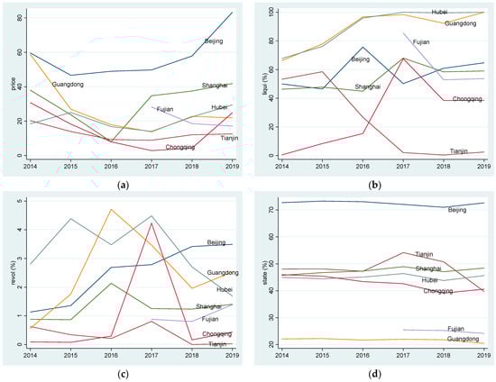
Figure 2.
(a) The historical carbon trading price trends in each pilot region over the years, measured via variable price; (b) the historical carbon market liquidity trends in each pilot region over the years, measured via variable liqui; (c) the historical carbon trading volume trends in each pilot region over the years, measured via variable price and measured via variable revol; (d) the historical level of administrative intervention trends in each pilot region over the years, measured via variable price and measured via the variable state.
4. Estimation of Treatment Effects
4.1. Baseline Model Estimation Results
Using the procedure described in Section 2.1, we first select the best prediction model for each CTP provincial-level region based on the CV criterion. Then, we construct the counterfactuals for the hypothetical ln(tce) and ln(ci) paths of each CTP region, assuming there was no implementation of the CTP policy. We estimate the OLS weights based on Step 4 using data from 2000 to 2013. The number of predictors and model fit results are reported in Table 3.
Table 3.
Results of the control group and model fit.
According to Table 3, the selected number of predictors ranges from 5 to 12. This demonstrates that the number of predictors in all predictive models does not exceed 12. Furthermore, all the predictive models have R-squared values above 0.97 and CVMSE below 0.012, indicating that all the predictive models perform well.
Next, we construct the counterfactuals for Beijing, Tianjin, Shanghai, Guangdong, Hubei, and Chongqing without the CTP policy treatment from 2014 to 2019 and construct the counterfactuals for Fujian without the CTP policy treatment from 2017 to 2019. Then, in Figure 1, we plot the actual post-treatment data, the predicted values of the counterfactuals, and the estimated treatment effects .
For Beijing, the upper panel of Figure 3a shows that the counterfactual path closely follows the actual path of ln(tce) before the implementation of the Beijing CTP policy. It is also noteworthy that the post-sample predictions closely match the actual turning points during the treatment period. For Tianjin, Shanghai, Guangdong, Hubei, Chongqing, and Fujian, the upper panels of Figure 3b–g, respectively, depict that the counterfactual paths closely trace the actual paths of ln(tce) before the implementation of the CTP policy; the post-sample predictions also closely match the actual turning points during the treatment period. These results further indicate that the counterfactual model fits the actual data quite well.
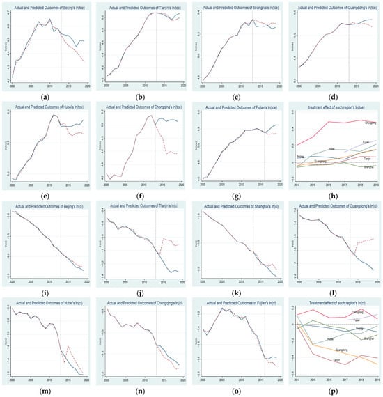
Figure 3.
(a) Actual and predicted outcomes of Beijing’s ln(tce); (b) actual and predicted outcomes of Tianjin’s ln(tce); (c) actual and predicted outcomes of Shanghai’s ln(tce); (d) actual and predicted outcomes of Guangdong’s ln(tce); (e) actual and predicted outcomes of Hubei’s ln(tce); (f) actual and predicted outcomes of Chongqing’s ln(tce); (g) actual and predicted outcomes of Fujian’s ln(tce); (h) estimated treatment effects of each provincial-level region’s ln(ci); (i) actual and predicted outcomes of Beijing’s ln(ci); (j) actual and predicted outcomes of Tianjin’s ln(ci); (k) actual and predicted outcomes of Shanghai’s ln(ci); (l) actual and predicted outcomes of Guangdong’s ln(ci); (m) actual and predicted outcomes of Hubei’s ln(ci); (n) actual and predicted outcomes of Chongqing’s ln(ci); (o) actual and predicted outcomes of Fujian’s ln(ci); (p) estimated treatment effects of each provincial-level region’s ln(ci). Notes. The blue solid line and red dashed line, respectively, represent actual and predicted outcomes and the vertical black dotted line indicates the year of the policy implementation excluding (h,p).
Furthermore, we can find from Figure 3a–g that the actual value curves for Beijing, Chongqing, and Fujian consistently remain higher than the fitted value curves, indicating that the CTP policy has a positive treatment effect on ln(tce) in these regions. In contrast, the actual value curve for Shanghai consistently remains lower than the fitted value curve while the actual value curves for Tianjin, Guangdong, and Hubei exhibit a trend of initially being lower than and later surpassing the fitted value curves. Hence, the CTP policy has a negative impact on ln(tce) in Shanghai and exhibits a suppressive effect initially, followed by a stimulative effect, in Tianjin, Guangdong, and Hubei. While the trends in the effects of the CTP policy are similar in Tianjin, Guangdong and Hubei, the timing of the turning point and the degree of the treatment effect vary.
The above findings suggest that the effects of the CTP policy on ln(tce) vary from region to region. As illustrated in Figure 3h, the treatment effect curves for Beijing, Chongqing, and Fujian consistently remain above zero while the treatment effect curve for Shanghai consistently remains below zero. On the contrary, the treatment effect curves for the remaining regions initially start below zero and then rise above it.
Regarding Beijing, in the lower section of Figure 3i, it is evident that the counterfactual trajectory closely follows the actual trajectory of ln(ci) before the implementation of the Beijing CTP policy. Remarkably, the post-sample predictions also align with the actual turning points during the treatment period. The upper sections of Figure 3j–o demonstrate that the counterfactual trajectory closely tracks the actual trajectory of ln(ci) before the implementation of the CTP policy for Tianjin, Shanghai, Guangdong, Hubei, Chongqing, and Fujian. Additionally, the post-sample predictions closely match the actual turning points during the treatment period. These findings further emphasize the strong fit of the counterfactual model to the actual data.
Furthermore, we can observe from Figure 3i–o that the actual value curves for Chongqing and Fujian are generally higher than the fitted value curves, indicating a positive effect of the CTP policy on ln(ci) in these two regions. Conversely, the actual value curves for the other five regions are generally lower than the fitted value curves, suggesting a negative effect of the CTP policy on ln(ci) in these regions.
The above conclusions imply that the impact of the CTP policy on ln(ci) differs across regions. As depicted in Figure 3p, the treatment effect curves for Chongqing and Fujian generally maintain a positive trend while the treatment effect curve for the remaining five regions tends to remain negative.
In a word, H1 is verified. This means that there are heterogeneous CTP policy effects across different pilot regions.
4.2. Results of Average Treatment Effect
According to Equation (5), we calculate the average treatment effect (ATE) of the CTP policy on ln(tce) and ln(ci) in each CTP provincial-level region as presented in Table 4.
Table 4.
Results of average treatment effect.
Table 4 contains data on the average treatment effect (ATE) on ln(tce) and ln(ci) for seven CTP provincial-level regions during the whole evaluation period divided into the first three-year period and second three-year period.
Panel A of Table 4 presents the ATE on ln(tce). For Beijing, Hubei, Chongqing, and Fujian, the ATE on ln(tce) is consistently positive throughout the entire evaluation period, indicating a positive average treatment effect on ln(tce). Taking Beijing as an example, the average projected ln(tce) without the CTP stands at 4.418 during the entire evaluation period. Therefore, the ATE on Beijing’s TCE growth rate is 8.2%. Furthermore, the ATE during the second three-year period is progressively higher than that of the first three-year period. For instance, in Beijing, the ATE for the first three-year period is 6.2% while the ATE increases to 10.2% for the second three-year period. In contrast, for Shanghai, the ATE for the entire evaluation period is consistently negative at −3.5%, with −3.9% and −3.0% in the first and second three-year periods, respectively. For Tianjin and Guangdong, there is a positive ATE for the entire evaluation period and the second three-year period, but it is slightly negative in the first three-year period. Taking Tianjin as an example, the ATE for the entire evaluation period is 1.7%, accompanied by a −1.9% ATE in the first three-year period and a 5.4% ATE in the second three-year period.
In Panel B of Table 4, we explore the ATE on ln(ci). Chongqing and Fujian exhibit positive ATE values of 11.9% and 8.2%, indicating a favorable impact on the growth rate of their CI. Furthermore, it is noteworthy that, excluding Chongqing and Fujian, the ATE of the CTP policy yields negative results for the remaining five regions. Among these regions, Tianjin and Guangdong experience relatively pronounced negative effects while the impact on Beijing, Shanghai, and Hubei is comparatively milder. Although all five regions exhibit negative ATE values, there are variations in the absolute magnitude of the ATE between the first and second three-year periods. Specifically, the absolute magnitude of the ATE for Hubei in the second three-year period is smaller than in the first three-year period. The absolute magnitude of the ATE for the other four regions in the second three-year period is larger than in the first three-year period.
In Panel C of Table 4, we explore the ATE on economic growth measured via the difference between ln(tce) and ln(ci). From the table, it shows that, except for the ATE in the first three years in Shanghai, the ATE of the CTP on economic growth in all pilot areas is positive. This indicates that the CTP exhibits a rebound effect on carbon emissions, which stems from the CTP promoting increased output and a rebound in energy consumption. Further analysis reveals that when the negative impact of the CTP on carbon intensity is weaker than the positive rebound effect of the CTP, the CTP will promote ln(tce). Conversely, when the negative impact of the CTP on carbon intensity is stronger than the positive rebound effect of the CTP, the CTP will facilitate a decrease in ln(tce).
In summary, based on the aforementioned analysis, we can classify the impact of CTPs on carbon emissions as belonging to three unique types. The first type involves reductions in both ln(tce) and ln(ci), exemplified by Shanghai. The second type pertains to a reduction in ln(ci) accompanied by a rise in ln(tce), as observed in Beijing, Tianjin, Guangdong, and Hubei. The third type entails an increase in both ln(tce) and ln(ci), as seen in Chongqing and Fujian.
4.3. Robust Analysis
- (1)
- Changing model parameters
In comparison with the baseline model, we conduct a thorough robustness analysis by examining various parameter-related aspects. Firstly, we replace the LASSO method with the forward method to select the suboptimal model, intending to evaluate whether the selection method affects the stability of the conclusions (Robust Model 1). The best method selects the suboptimal model with the highest R-squared value for each specified number of predictors. Secondly, we specify the criteria for selecting the optimal model from among all the suboptimal models as AICC, AIC, BIC, and MBIC. This allows us to investigate whether the estimation results remain robust across different criterion selections (Robust Model 2–4). Thirdly, we employ the LASSO method instead of the OLS method to estimate the optimal model for counterfactual prediction. The LASSO regression sets a grid for lambda, known as the tuning or penalty parameter, and fits the corresponding LASSO regressions on that grid as the suboptimal models (Robust Model 5). Then, we systematically decrease the number of explanatory variables to assess how the inclusion of explanatory variables influences the enhancement of predictive accuracy (Robust Model 6–8). Lastly, we adjust the sample’s initial year from 2000 to 2002, enabling us to evaluate the impact of the pre-policy implementation time duration on the fitting results (Robust Model 9).
We estimate the nine robustness models mentioned above and examine the number of consistent directional estimates with the baseline model, as shown in Table 5. From Table 5, we can observe that the estimates of most robustness models are consistent with the estimates of the baseline model. At least seven out of the nine models exhibit results consistent with the baseline model. This suggests that the estimates of the baseline model remain robust against variations in model parameter selections, indicating that the results of the baseline model are reliable.
Table 5.
Number of consistent directional estimates between robustness models and baseline models.
- (2)
- Analysis of the impacts of spillover effects
The results of the ATEs reported in Table 4 are under the condition of excluding spillover effects which contain the neighboring effect and pairwise-assisted effect. The two types of spillover effects have different origins, with the former stemming from spatial geographical spillover and the latter originating from policy-driven impacts.
To assess whether the scope of the spillover effect affects the stability of the baseline model’s conclusions, we only use the neighboring effect and pairwise-assisted effect to measure the spillover effect. The SignN and SignP reported in Table indicate whether the sign of the ATE is consistent with the baseline model after excluding the neighboring effect and pairwise-assisted effect. We can observe that whether using only the neighboring effect or the pairwise-assisted effect, the sign of the ATE remains consistent with the baseline model. This indicates that the conclusions of the baseline model are relatively robust against the scale of measuring spillover effects.
Next, we consider the impacts of spillover effects. Columns 5 and 10 in Table 6 report the ATE on ln(tce) and ln(ci) without excluding the spillover effects, referred to as ATES. We can observe from columns 4 and 9 in Table 6 that, except for Tianjin, the signs of ATEs in the other six pilot regions are consistent with the baseline model. This suggests that the conclusions of our baseline model are relatively robust against spillover effects. Furthermore, we calculate the difference (∆ATE) between the ATES and the ATE from the baseline, as reported in columns 6 and 11 in Table 6. We can observe that the ∆ATE ranges from −0.281 to 0.097, indicating a variation in spillover effects among pilot regions. In summary, it is evident that while the consideration of spillover effects has a relatively minor impact on the sign of the ATE, it significantly affects the magnitude of the ATE. Therefore, it is necessary to account for spillover effects when analyzing the factors that influence ATE heterogeneity.
Table 6.
Comparative analysis of ATEs with and without spillover effects.
4.4. Factors Affecting the Disparity of CTP Policy Impacts
Based on the above analysis, we can preliminarily find that the carbon market conditions in the pilot regions vary significantly with clear differences. These differences may be the reasons for the disparity in the impacts of the CTP policy on carbon emissions. To validate this hypothesis, we further employ multi-level ordered regression models, including multi-level ordered logit models and multi-level ordered probit models. The dependent variable consists of 0, 1, and 2, corresponding to the three categories of the ATE results mentioned earlier. Specifically, 0 represents the type where both the ATE on ln(tce) and the ATE on ln(ci) are greater than 0; 1 represents the type where the ATE on ln(tce) is greater than 0 while the ATE on ln(ci) is less than 0; and 2 represents the type where both the ATE on ln(tce) and the ATE on ln(ci) are less than 0.
The results of multi-level ordered regression are reported in Table 7. From Table 7, we can find the following conclusions:
Table 7.
Results of multi-level ordered regression models.
The price variable is statistically significant at the 5% level. The negative coefficient (−0.099 in the mologit model and −0.049 in the moprobit model) indicates that as carbon prices increase, there is a higher likelihood of falling into a lower ATE category. In other words, higher carbon prices are associated with positive ATEs on ln(tce) and ln(ci). The above analysis clarifies that high carbon emission costs are not conducive to achieving reduction both in carbon emission and intensity.
The liqui variable exhibits statistical significance at the 5% level, with a positive coefficient of 0.064 in the mologit model and 0.032 in the moprobit model. This finding implies that an augmented level of liquidity within the carbon market is linked to an increased probability of being classified into a higher ATE category. In essence, heightened carbon market liquidity is indicative of a negative impact on ln(tce) and ln(ci). This suggests that enhancing the vitality of the carbon market can help promote a decrease in both total carbon emissions and carbon intensity.
The revol variable appears to be insignificant in either model statistically. This suggests that the annual trading volume relative to the region’s total emissions does not have a significant impact on the classification of ATE categories.
The state variable, with a positive coefficient of 0.224 in the mologit model and 0.134 in the moprobit model, demonstrates statistical significance at the 10% level. This implies that a higher proportion of state-owned enterprise assets is correlated with an increased probability of belonging to a higher ATE category. In essence, regions with a greater presence of state-owned enterprises tend to exhibit more pronounced negative impacts on ln(tce) and ln(ci). This indicates that the government plays an active role in carbon market development, and not all forms of administrative intervention are detrimental. Appropriately proactive intervention in the carbon market can contribute to a reduction in both total carbon emissions and carbon intensity.
In addition to the above-mentioned carbon market variables, we also find that a higher proportion of technological innovation and industrialization has a negative impact on ln(tce) and ln(ci) while a higher proportion of population scale has a positive impact on ln(tce) and ln(ci). Furthermore, the level of economic development has a non-linear effect on the ATE. An increase in the level of economic development will result in a positive impact on ln(tce) and ln(ci) when the level of economic development is low, while it will have a negative impact on ln(tce) and ln(ci) when the level of economic development is high.
In summary, carbon market trading prices, market liquidity, and government intervention significantly affect the CTP policy effects and H2 is confirmed.
5. Discussion
This paper employs RCM to assess the carbon emission reduction effects of each carbon trading pilot area and provides empirical evidence for the heterogeneous effects of China’s CTP on carbon emissions. The research enriches existing studies from the perspective of heterogeneous effects. While numerous studies [,,,,,,,] have analyzed the carbon emission effects of CTPs, their conclusions built on homogeneous policy effects, often yielding results in an average sense. Our paper emphasizes the operational modes of carbon markets and the environmental differences faced by each pilot area. The research reveals varied changes in the speed of carbon emission growth and carbon intensity after the implementation of CTP policies in different areas. For example, Shanghai’s implementation of the CTP policy has shown promising carbon reduction effects. The research conclusions were validated through a series of robustness tests and underscored the necessity of evaluating heterogeneous policy effects, highlighting the value of this study. Additionally, it is worth noting that Yi et al. (2020) [] also observed differentiated policy effects among pilot areas. However, their assessment strategy involved grouping the CTP areas, which fails to reflect the time variability of policy effects. To improve this, Table 4 in this paper presents the effect values of each pilot area during different periods post-policy implementation, aiding in understanding the heterogeneity of policy effects in both spatial and temporal dimensions among pilot areas.
Furthermore, existing research has often focused on policy effect evaluations, frequently overlooking the analysis of factors contributing to policy effect differentiation. In fact, exploring the reasons behind the differentiation of policy effects among pilot areas is crucial. This exploration provides policy directions for adopting adjusted measures to strengthen policy effects. Specifically, this paper explains the differentiation of policy effects from the perspectives of market mechanisms and administrative intervention. Efficient ways include moderately adjusting carbon emission trading prices in pilot areas, enhancing carbon market liquidity, and effectively leveraging government roles, which can promote carbon market effectiveness in pilot areas and thus ensure the orderly operation of the carbon market for emissions reduction.
The research conclusions of this paper both provide support for analyzing the effectiveness of the carbon market and offer directions for future research. Apart from analyzing causal factors (as presented in Table 7), it is necessary to place carbon reduction targets within the broader economic development framework considering the heterogeneous effects mentioned above. This involves clarifying the relationship between the effects of carbon trading pilot policies and factors such as energy consumption, environmental pollution, and economic growth. Consequently, through optimizing carbon trading mechanisms and coordinating government intervention efforts, there can be synchronized governance for pollution reduction, carbon mitigation, and achieving high-quality economic development.
6. Conclusions and Policy Recommendations
6.1. Conclusions
Based on the construction of China’s carbon trading market and using panel data from 30 provincial-level regions between 2000 and 2019, this study employs causal identification to assess the carbon emission reduction effects of each CTP policy pilot area by adopting the RCM introduced by Hsiao et al. (2012) []. The conclusions of this study are as follows:
Firstly, the effects of China’s CTP policy on carbon emission reduction vary significantly among different pilot areas. In terms of the rate of total carbon emissions, the treatment effect curves for Beijing, Chongqing, and Fujian consistently exhibit positive values, while the treatment effect curve for Shanghai consistently remains negative. On the other hand, the treatment effect curves for the remaining regions initially start with negative values but eventually shift to positive values. In terms of the rate of carbon emission intensity, the treatment effect curves for Chongqing and Fujian generally display a positive trend, whereas the treatment effect curve for the other five regions tends to remain negative.
Secondly, the effects of the CTP policy on carbon emissions can be categorized into three distinct types. The first type includes reductions in both total carbon emissions and carbon emission intensity, as demonstrated by Shanghai. The second type involves a decrease in carbon emission intensity accompanied by an increase in total carbon emissions, as observed in Beijing, Tianjin, Guangdong, and Hubei. The third type encompasses an increase in both total carbon emissions and carbon emission intensity, as evidenced in Chongqing and Fujian.
Thirdly, while the magnitude of the effects varies among the pilot regions, the CTP policy has significantly boosted economic growth in all pilot areas. If the positive impact of the CTP policy on economic growth is stronger than its negative impact on carbon emission intensity, the CTP policy has a promoting effect on total carbon emissions. Conversely, if the positive impact of the CTP policy on economic growth is weaker than its negative impact on carbon emission intensity, the CTP has a restraining effect on total carbon emissions.
Lastly, both market mechanisms and administrative forces play crucial roles in the heterogeneous effects of the CTP policy on carbon emission reduction. Among the market mechanisms, both carbon price and carbon liquidity significantly influence the heterogeneous effects of the CTP policy on carbon emission reduction. In contrast to European and American carbon markets, China’s low carbon prices and high liquidity have had a positive impact on carbon emission reduction. Additionally, administrative interventions by the state, such as through state-owned enterprises, have played a constructive role in the carbon reduction effects of the CTP policy. In addition to the factors mentioned above, technological innovation is an effective way to enhance the carbon emission reduction effects of the CTP policy. Furthermore, the arrival of a turning point in China’s population scale is also conducive to improving the carbon reduction effects of the CTP policy.
6.2. Policy Recommendations
The research conclusions of this paper provide empirical evidence for enhancing the effectiveness of the carbon market and formulating differentiated policies for each pilot area based on their strengths. The following policy implications are presented:
First and foremost, guided by the dual carbon goals, tailor the design of the carbon market system to fit the characteristics of the industries in each pilot area. As one of the most important means for addressing carbon reduction, the carbon market has exerted positive effects in certain pilot areas. For instance, in Shanghai, both the volume and intensity of carbon emissions show negative effects. This is largely associated with Shanghai’s dedication to creating a green and low-carbon supply chain and closely supporting relevant enterprises in their green transformation, effectively reducing corporate carbon emissions. Therefore, other regions can, based on their industrial characteristics, include more high-carbon-emission industries in carbon emission trading and optimize the design of the carbon market system, thus aiming to achieve the dual reduction goals in carbon emission volume and intensity.
Secondly, when evaluating the carbon emission reduction effects of CTP policy, it is essential to analyze both the carbon intensity reduction effect and the energy rebound effect. While CTP policy may promote improvements in carbon productivity and carbon intensity reduction, they may also lead to increased energy consumption and a rebound in carbon emissions through the expansion of output scales.
Thirdly, based on the analysis of factors influencing differentiation effects, this paper suggests that each pilot area should pay attention to key factors influencing policy effects, strengthen the carbon market trading mechanisms, adjust administrative intervention, and maximize the effectiveness of the carbon market from the perspective of coordinated environmental, population, and economic development. For example, during the bidding process for carbon quotas by enterprises, regulating the transaction price should be considered to prevent exacerbating corporate burdens. Additionally, leveraging the U-shaped relationship between per capita GDP and policy effects and accelerating corporate green transformation can achieve coordinated development in economic growth and low carbon emissions after reaching a certain level of economic growth. Moreover, considering the broader context of China’s declining population growth, each pilot area can integrate carbon emission trading policies with population policies to regulate the effects of low-carbon policies.
Lastly, whether it is the assessment of CTP policy effectiveness or the design of specific policy structures, it is important to consider the policy’s spatial spillover effects. These spillover effects arise not only from natural geographical spillovers but also from spatial spillovers generated by national administrative policies, such as inter-provincial pairing assistance policies.
Author Contributions
Conceptualization, F.L. and W.W.; methodology, F.L.; software, Y.F.; validation, F.L., Y.F. and W.W.; formal analysis, F.L.; investigation, F.L.; resources, F.L.; data curation, Y.F.; writing—original draft preparation, F.L.; writing—review and editing, Y.F.; visualization, F.L.; supervision, W.W.; project administration, W.W.; funding acquisition, W.W. All authors have read and agreed to the published version of the manuscript.
Funding
This research was funded by the National Natural Science Foundation of China, grant number 72273019.
Institutional Review Board Statement
Not applicable.
Informed Consent Statement
Not applicable.
Data Availability Statement
All data sources have been provided in the text where readers may download the original source data.
Conflicts of Interest
The authors declare no conflict of interest.
References
- Ahmad, M.; Zhao, Z.-Y.; Li, H. Revealing stylized empirical interactions among construction sector, urbanization, energy consumption, economic growth and CO2 emissions in China. Sci. Total. Environ. 2018, 657, 1085–1098. [Google Scholar] [CrossRef] [PubMed]
- Michieka, N.M.; Fletcher, J.; Burnett, W. An empirical analysis of the role of China’s exports on CO2 emissions. Appl. Energy 2013, 104, 258–267. [Google Scholar] [CrossRef]
- Chevallier, J.; Nguyen, D.K.; Reboredo, J.C. A conditional dependence approach to CO2-energy price relationships. Energy Econ. 2019, 81, 812–821. [Google Scholar] [CrossRef]
- Li, W.; Lu, C. The research on setting a unified interval of carbon price benchmark in the national carbon trading market of China. Appl. Energy 2015, 155, 728–739. [Google Scholar] [CrossRef]
- Chen, X.; Lin, B. Towards carbon neutrality by implementing carbon emissions trading scheme: Policy evaluation in China. Energy Policy 2021, 157, 112510. [Google Scholar] [CrossRef]
- Zhou, C.; Qi, S. Has the pilot carbon trading policy improved China’s green total factor energy efficiency? Energy Econ. 2022, 114, 106268. [Google Scholar] [CrossRef]
- Hong, Q.; Cui, L.; Hong, P. The impact of carbon emissions trading on energy efficiency: Evidence from quasi-experiment in China’s carbon emissions trading pilot. Energy Econ. 2022, 110, 106025. [Google Scholar] [CrossRef]
- Yu, H.; Jiang, Y.; Zhang, Z.; Shang, W.-L.; Han, C.; Zhao, Y. The impact of carbon emission trading policy on firms’ green innovation in China. Financial Innov. 2022, 8, 55. [Google Scholar] [CrossRef]
- Xiao, Y.; Huang, H.; Qian, X.-M.; Chen, L. Can carbon emission trading pilot facilitate green development performance? Evidence from a quasi-natural experiment in China. J. Clean. Prod. 2023, 400, 136755. [Google Scholar] [CrossRef]
- Chen, Z.; Zhang, X.; Chen, F. Do carbon emission trading schemes stimulate green innovation in enterprises? Evidence from China. Technol. Forecast. Soc. Chang. 2021, 168, 120744. [Google Scholar] [CrossRef]
- Huang, D.; Chen, G. Can the Carbon Emissions Trading System Improve the Green Total Factor Productivity of the Pilot Cities?—A Spatial Difference-in-Differences Econometric Analysis in China. Int. J. Environ. Res. Public Health 2022, 19, 1209. [Google Scholar] [CrossRef] [PubMed]
- Chen, Z.; Song, P.; Wang, B. Carbon emissions trading scheme, energy efficiency and rebound effect–Evidence from China’s provincial data. Energy Policy 2021, 157, 112507. [Google Scholar] [CrossRef]
- Liu, B.; Ding, C.J.; Hu, J.; Su, Y.; Qin, C. Carbon trading and regional carbon productivity. J. Clean. Prod. 2023, 420, 138395. [Google Scholar] [CrossRef]
- Xie, Y.; Guo, Y.; Zhao, X. The impact of carbon emission trading policy on energy efficiency—Evidence from China. Environ. Sci. Pollut. Res. 2023, 30, 105986–105998. [Google Scholar] [CrossRef] [PubMed]
- Tao, M.; Goh, L.T. Effects of Carbon Trading Pilot on Carbon Emission Reduction: Evidence from China’s 283 Prefecture-Level Cities. Chin. Econ. 2022, 56, 1–24. [Google Scholar] [CrossRef]
- Pan, X.; Pu, C.; Yuan, S.; Xu, H. Effect of Chinese pilots carbon emission trading scheme on enterprises’ total factor productivity: The moderating role of government participation and carbon trading market efficiency. J. Environ. Manag. 2022, 316, 115228. [Google Scholar] [CrossRef]
- Yang, X.; Zhang, J.; Bi, L.; Jiang, Y. Does China’s Carbon Trading Pilot Policy Reduce Carbon Emissions? Empirical Analysis from 285 Cities. Int. J. Environ. Res. Public Health 2023, 20, 4421. [Google Scholar] [CrossRef]
- Xia, Q.; Li, L.; Dong, J.; Zhang, B. Reduction Effect and Mechanism Analysis of Carbon Trading Policy on Carbon Emissions from Land Use. Sustainability 2021, 13, 9558. [Google Scholar] [CrossRef]
- Xuan, D.; Ma, X.; Shang, Y. Can China’s policy of carbon emission trading promote carbon emission reduction? J. Clean. Prod. 2020, 270, 122383. [Google Scholar] [CrossRef]
- Tian, G.; Yu, S.; Wu, Z.; Xia, Q. Study on the Emission Reduction Effect and Spatial Difference of Carbon Emission Trading Policy in China. Energies 2022, 15, 1921. [Google Scholar] [CrossRef]
- Zhang, Y.; Li, S.; Luo, T.; Gao, J. The effect of emission trading policy on carbon emission reduction: Evidence from an inte-grated study of pilot regions in China. J. Clean. Prod. 2020, 265, 121843. [Google Scholar] [CrossRef]
- Lan, J.; Li, W.; Zhu, X. The road to green development: How can carbon emission trading pilot policy contribute to carbon peak attainment and neutrality? Evidence from China. Front. Psychol. 2020, 13, 962084. [Google Scholar] [CrossRef] [PubMed]
- Yi, L.; Bai, N.; Yang, L.; Li, Z.; Wang, F. Evaluation on the effectiveness of China’s pilot carbon market policy. J. Clean. Prod. 2020, 246, 119039. [Google Scholar] [CrossRef]
- Shen, J.; Tang, P.; Zeng, H. Does China’s carbon emission trading reduce carbon emissions? Evidence from listed firms. Energy Sustain. Dev. 2020, 59, 120–129. [Google Scholar] [CrossRef]
- Li, Z.; Wang, J. Spatial spillover effect of carbon emission trading on carbon emission reduction: Empirical data from pilot regions in China. Energy 2022, 251, 123906. [Google Scholar] [CrossRef]
- Liu, Y.; Liu, S.; Shao, X.; He, Y. Policy spillover effect and action mechanism for environmental rights trading on green in-novation: Evidence from China’s carbon emissions trading policy. Renew. Sust. Energ. Rev. 2022, 153, 111779. [Google Scholar] [CrossRef]
- Yu, W.; Luo, J. Impact on Carbon Intensity of Carbon Emission Trading—Evidence from a Pilot Program in 281 Cities in China. Int. J. Environ. Res. Public Health 2022, 19, 12483. [Google Scholar] [CrossRef]
- Li, Z.; Wang, J. Spatial emission reduction effects of China’s carbon emissions trading: Quasi-natural experiments and policy spillovers. Chin. J. Popul. Resour. Environ. 2021, 19, 246–255. [Google Scholar] [CrossRef]
- Wang, X.Q.; Su, C.W.; Lobonţ, O.R.; Li, H.; Nicoleta-Claudia, M. Is China’s carbon trading market efficient? Evidence from emissions trading scheme pilots. Energy 2022, 245, 123240. [Google Scholar] [CrossRef]
- Lin, B.; Huang, C. Analysis of emission reduction effects of carbon trading: Market mechanism or government intervention? Sustain. Prod. Consum. 2022, 33, 28–37. [Google Scholar] [CrossRef]
- Hsiao, C.; Ching, H.S.; Wan, S.K. A Panel Data Approach for Program Evaluation: Measuring the Benefits of Political and Economic Integration of Hong Kong with Mainland China. J. Appl. Econ. 2012, 27, 705–740. [Google Scholar] [CrossRef]
- Hsiao, C.; Zhou, Q.K. Panel Parametric, Semiparametric, and Nonparametric Construction of Counterfactuals. J. Appl. Economet. 2019, 34, 463–481. [Google Scholar] [CrossRef]
Disclaimer/Publisher’s Note: The statements, opinions and data contained in all publications are solely those of the individual author(s) and contributor(s) and not of MDPI and/or the editor(s). MDPI and/or the editor(s) disclaim responsibility for any injury to people or property resulting from any ideas, methods, instructions or products referred to in the content. |
© 2023 by the authors. Licensee MDPI, Basel, Switzerland. This article is an open access article distributed under the terms and conditions of the Creative Commons Attribution (CC BY) license (https://creativecommons.org/licenses/by/4.0/).