Abstract
Existing tunnel defect detection methods often lack repeated inspections, limiting longitudinal analysis of defects. To address this, we propose a multi-information fusion approach for continuous defect monitoring. Initially, we utilized the You Only Look Once version 7 (Yolov7) network to identify defects in tunnel lining videos. Subsequently, defect localization is achieved with Super Visual Odometer (SuperVO) algorithm. Lastly, the SuperPoint–SuperGlue Matching Network (SpSg Network) is employed to analyze similarities among defect images. Combining the above information, the repeatability detection of the disease is realized. SuperVO was tested in tunnels of 159 m and 260 m, showcasing enhanced localization accuracy compared to traditional visual odometry methods, with errors measuring below 0.3 m on average and 0.8 m at maximum. The SpSg Network surpassed the depth-feature-based Siamese Network in image matching, achieving a precision of 96.61%, recall of 93.44%, and F1 score of 95%. These findings validate the effectiveness of this approach in the repetitive detection and monitoring of tunnel defects.
1. Introduction
With the rapid development of tunnel traffic in recent years, public attention has shifted from tunnel construction to maintenance [1]. However, due to the influence of internal and external variables such as long-term cyclic stress, groundwater, and poor construction, tunnels unavoidably develop a variety of visible tunnel lining diseases [2]. These diseases, such as cracks, leakage, and corrosion, will shorten the tunnel’s service life. If the disease cannot be managed in time, it will worsen and eventually cause the tunnel to collapse, resulting in a crisis of personnel safety. Therefore, early and accurate monitoring of tunnel lining diseases is essential.
The conventional approach to detecting tunnel surface disease primarily depends on labor, which is subjective, ineffective, and lacks precision [3]. Therefore, to reduce the use of manpower, the use of automated equipment for tunnel lining surface inspection is becoming the mainstream of modern tunnel operation and maintenance [4]. For example, Li et al. developed a rail-mounted device for capturing images [3]. The system is equipped with eight high-resolution line-scanning cameras and nine linear light sources. This configuration enables precise diagnosis of numerous diseases. Liao et al. introduced a novel mobile tunnel inspection system (MTIS) [5], which combines numerous sensors such as CCD cameras, laser scanners, and IMUs. These methods are mostly utilized for subway tunnels and highway tunnels, employing image-processing techniques based on deep learning. They exhibit great identification accuracy and robustness.
However, tunnel lining disease is a progressive and continuous procedure. Prolonged observation is necessary to comprehend the progression before the tunnel O&M management decides on whether to address the disease [4]. It is rare to do repetitive examinations for tunnel diseases or compare the results of various inspections. Thus, this paper presents a method for repetitive inspections of tunnel lining diseases. The contributions of this research are summarized below:
- (1)
- This study proposes an approach to recognize repeated tunnel lining diseases using multi-information fusion. It integrates location information, mileage information, and image similarity information.
- (2)
- Designed the SuperVO algorithm and devised a technique to mitigate the accumulation of errors by utilizing distinguishable marks. This method enables the localization task to be performed solely with a monocular camera, even in tunnel videos with limited texture and repetitive patterns.
- (3)
- Designed the SpSg Network, which enables the comparison of tunnel lining images acquired at different times, angles, and illumination conditions.
- (4)
- The effectiveness of our method has been demonstrated through practical experiments in real tunnels, offering a reliable and intelligent approach for detecting tunnel diseases and conducting long-term monitoring.
The organization of this article is structured as follows. Section 2 provides an overview of the latest studies on disease detection, localization, and matching. Section 3 provides a concise summary of our approach. Section 4 conducted experiments to evaluate the technique we proposed. Finally, the conclusion and future work are discussed.
2. Related Works
This chapter presents investigations relating to defect detection, localization, and image matching, respectively.
2.1. Defect Detection
Presently, tunnel disease is primarily detected through manual inspections. However, this method is objective and inefficient. In contrast to human inspections, traditional digital image processing is more efficient, and primarily utilizes techniques such as image frequency domain filtering, histogram thresholding, and intensity thresholding. For instance, Qu et al. [6] employed the percolation method, which utilizes the gray value’s consistency between neighboring pixels as the criterion for identifying crack pixels. Amhaz et al. [7] introduced a crack identification method that relies on the minimum path, taking into account the properties of crack continuity and low intensity. Unfortunately, the interiors of tunnels are complex and inadequately illuminated, including backgrounds such as lining joints, bolt holes, stains, and cables. Traditional digital image processing algorithms are susceptible to noise and lack robustness, thus requiring an enhancement of the detection accuracy.
With the increasing popularity of artificial intelligence, numerous academics have turned their attention towards deep learning. Su et al. [8] investigated the mechanism of spalling diseases and proposed a BP neural network for spalling recognition based on AE characteristics before spalling failure. Zhou et al. [2] enhanced the YOLOv4 model and introduced a real-time system for detecting tunnel diseases. Xue et al. [9] introduced a low-cost and effective method for automatically detecting and precisely measuring leaks in subway tunnels. The tunnel’s three-dimensional reconstruction is achieved by the Structure From Motion (SFM) technique. Additionally, the leakage in the image is segmented using Mask R-CNN. Zhao et al. [10] enhanced the PANet and proposed a method for quantifying cracks. A morphological closure process is incorporated into the semantic branching network of PANet to guarantee the consistency of cracks. Yet, these technologies mainly concentrate on identifying diseases in subway tunnels and utilize large-scale equipment to generate high-quality images. Thus, they are unsuitable for usage in restricted areas such as escape passages or cable channels.
2.2. Defect Localization
Precise identification of the disease’s position in the tunnel is crucial for daily management. However, due to the obstruction of satellite signals by reinforced concrete, tunnel localization has always been a difficult task. Most tunnel location methods use odometry or INS (Inertial Navigation System). For instance, YANG et al. [11] introduced a precise navigation technique that combines an inertial navigation system, odometry, and Doppler radar. Schaer et al. [12] proposed a method for error correction using control points in subway tunnels. However, the approach may fail if the tunnel lacks control point information. Du et al. [13] used an odometer to localize the section and then corrected the data by the longitudinal joints of the tunnel tube lining. H. Kim et al. [14] examined the localization methods of self-driving robots in underground mines using IMU and LiDAR, as well as both together, and found that IMU plus LiDAR had the highest accuracy.
These approaches employ expensive equipment like LIDAR or need calibration and connection debugging for multiple devices, which makes them difficult to use. Thus, we solely employed a monocular camera to estimate the mileage. We previously proposed an image enhancement method [4] to boost image features and optimize visual odometry results using the Kalman filter. However, the localization accuracy in real tunnels still needs to be improved. So, we introduced SuperPoint [15] and presented SuperVO.
2.3. Image Matching
Image matching is a critical task in various vision applications which recognize the same or similar structure/content from two or more images [16]. Image matching can be classified into two main categories: traditional methods and deep learning methods [17]. Traditional image matching techniques included feature-based and template-based methods. Famous algorithms in feature-based image matching approaches include SIFT [18], SURF [19], ORB [20], RIFT [21], and their derivative methods. Representative template matching algorithms include Fast-Match [22], MSPD, [23] and Deep-Matching [24]. However, these methods are tailored for particular situations and are not suitable for tunnel scenarios. With the deep development of neural networks, an increasing number of deep learning methods are being utilized in the domain of image matching. The methods can be categorized into two groups, namely Patch Descriptors and Dense Descriptors. Patch-based methods employ batches of image pairs to train neural networks. For example, Chopra et al. [25] used a Siamese Network to learn the similarity of image pairs for face recognition. Zhang et al. [26] discovered that employing deep features can achieve better image matching results. The Dense Descriptors method, on the other hand, involves learning pixel-level features in the image. SuperPoint [15] learns a precise representation by randomly selecting the single responsiveness and simultaneously produces the locations and descriptors of keypoints using two distinct branches. Gleize et al. [27] introduced Simple Learned Keypoints (SiLK), a self-supervised method that effectively extracts discriminative keypoints.
Nevertheless, the appropriate selection for the tunnel scene remains uncertain. Hence, to create an appropriate image matching method for tunnel scenes, we proposed the SuperPoint–SuperGlue Matching Network. This network improved the existing feature-based method by incorporating SuperPoint and SuperGlue [28]. It can accomplish the matching of tunnel lining images across different times, viewpoints, and illumination conditions.
3. Materials and Methods
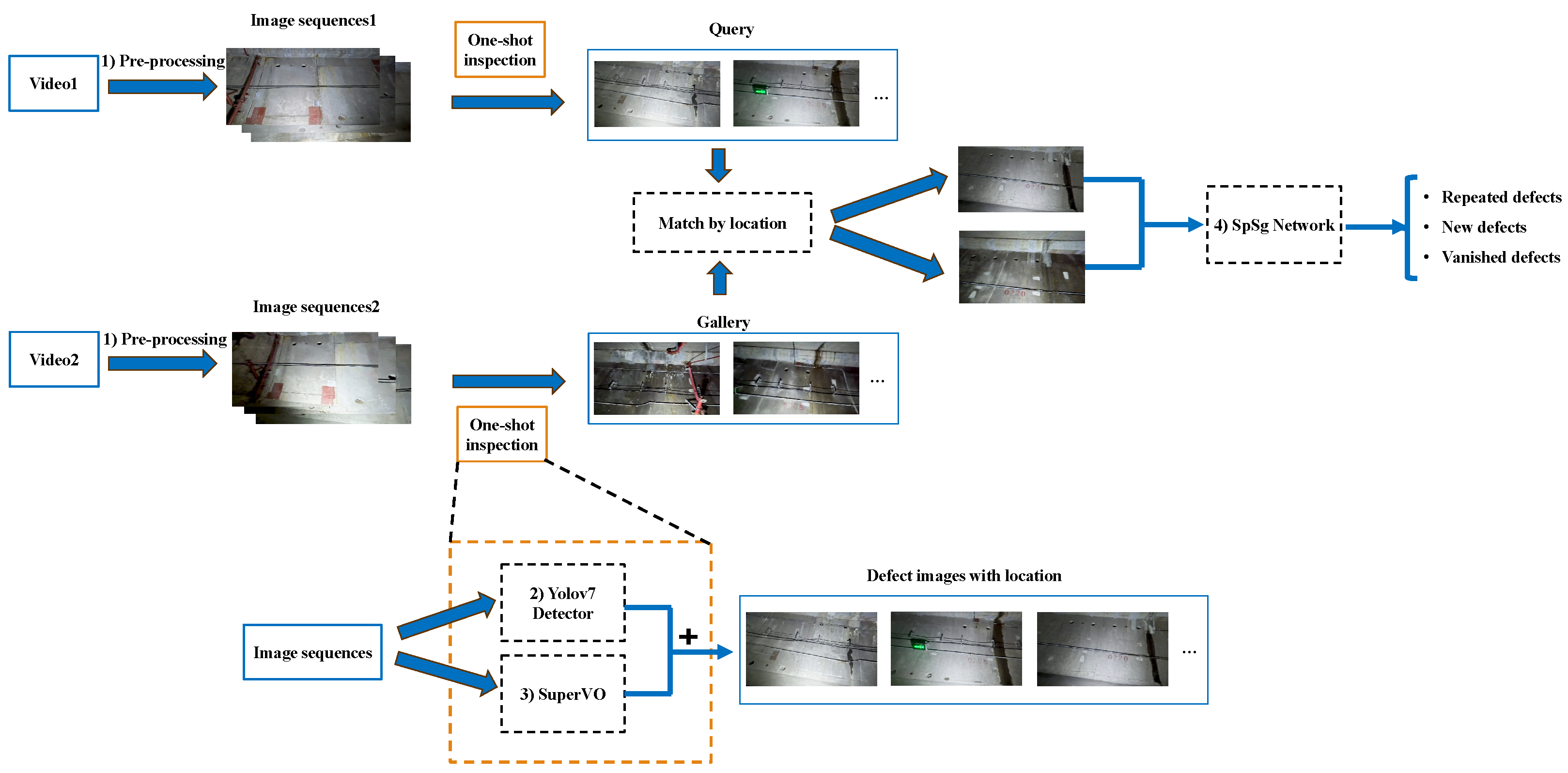
We proposed a tunnel disease localization and matching system based on multi-information fusion. This system is capable of detecting diseases repeatedly and accurately determining the count of new, repeated, and vanished diseases. The system analyzes tunnel inspection videos from various periods, as illustrated in Figure 1.
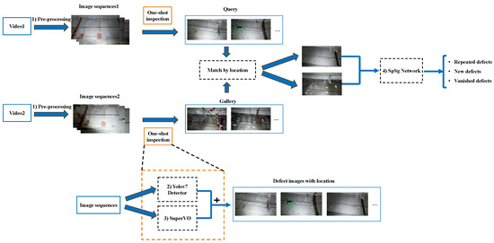
Figure 1.
Framework of localization and matching system based on multi-information fusion.
After acquiring Video1 and Video2, which were recorded at different times, we begin with the preprocessing to generate a sequence of video frames. Subsequently, the disease images, along with their corresponding location information, are obtained via the one-shot inspection procedure. The one-shot inspection process is shown inside the yellow dashed box. Initially, the video frames are inputted into the Yolov7 detector [29] to extract the disease images. Simultaneously, the SuperVO is utilized to obtain the odometer information. The disease images captured by Video1 are referred to as the Query. The disease images obtained from Video2 are referred to as the Gallery.
Subsequently, we employ a location-based filtering technique to compare the disease images in the Query against those in the Gallery. This process allows us to identify images that share similar locations to the query. The resulting neighboring disease images are then inputted into the SpSg Network for image matching. Images in the query that match the gallery images are repeat diseases. New diseases are considered if the disease image cannot be found in the Gallery. The disease images that remain in the Gallery are classified as diseases that resolve after repair. The method enables the continuous detection of defects and the long-term monitoring of tunnel structural health. The following section introduces system components in detail: (1) video preprocessing; (2) Yolov7 detector; (3) SuperVO visual odometer; and (4) the SpSg network.
3.1. Video Preprocessing
The raw video has severe radial distortion because we used an ultra-wide angle lens to shoot the tunnel surface from a close distance to get a wide field of view. The original video also has low contrast due to poor tunnel illuminations. Thus, preprocessing is necessary before detection and localization. Figure 2 illustrates the preprocessing steps. The 22.0 version of Premiere Pro software performed original video de-distortion and brightness adjustment. We fixed 20 frames to extract one image from the video to reduce redundancy and omissions. After preparing the video, we obtained the following image sequence.
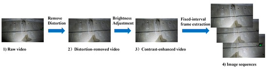
Figure 2.
Video preprocessing process.
3.2. Yolov7 Detector
The Yolo family is a very efficient and flexible one-stage object detector. It has just been updated to the Yolov9 [30]. We utilize the Yolov7 due to its simplicity of training and excellent detection results for our dataset. The network employs a reparameterization technique known as RepConv. This technique transforms the multi-branch convolution module used in training into a single 3 × 3 convolution during inference. This improvement enhances the speed of inference and simplifies the deployment process. Once the image sequence is processed by the Yolov7 detector, we can obtain images that contain diseases.
3.3. SuperVO Algorithm
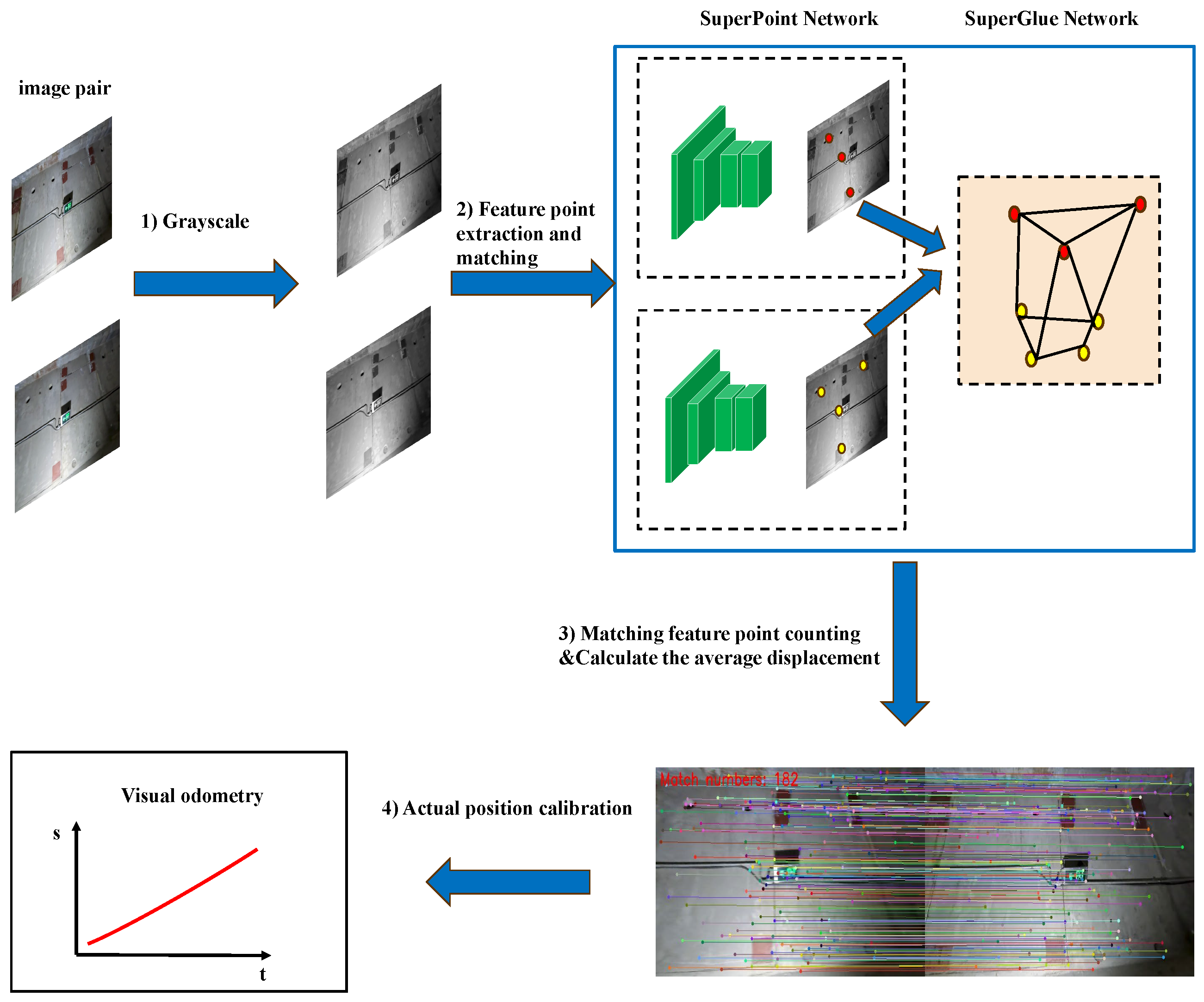
Visual odometry requires images that include appropriate light intensity and a relatively high level of texture. However, the tunnel does not have enough illuminations and there are not many features on the tunnel surface. The usual visual odometry method does not work well. Hence, we used the SuperPoint feature point and SuperGlue matching network together to create the SuperVO. Figure 3 illustrates the overall procedure of the SuperVO.
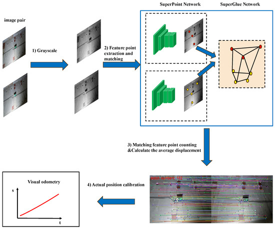
Figure 3.
SuperVO flow.
At first, we applied a grayscale transformation to the input images. The weighted average method was employed to execute grayscaling, as demonstrated in Equation (1). In this equation, represents the calculated grayscale value, while , , and denote the values of the red, green, and blue channels, respectively.
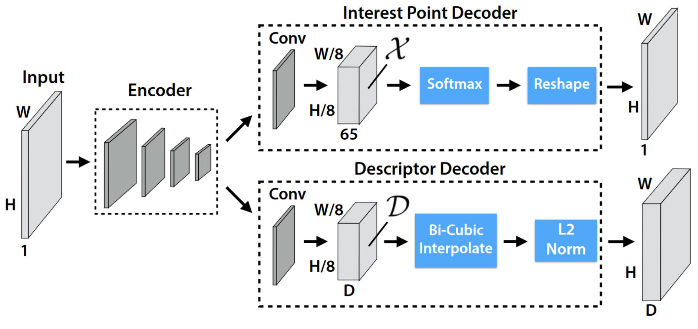
Secondly, SuperPoint and SuperGlue networks extract and match feature points with neighboring grayscale images. The SuperPoint network is a self-supervised network that extracts feature points and descriptors. The network has a Shared Encoder and two Decoder Heads, as shown in Figure 4. The Shared Encoder uses convolutional, pooling, and nonlinear activation functions to encode a grayscale image and output a feature map , where and . The first Decoder Head, the Interest Point Decoder, predicts keypoints. Convolution is used to turn the feature map into a -sized . The 65 channels correspond to localized, non-overlapping 8 × 8-pixel grid sections and a “no points of interest” zone. Furthermore, softmax and reshape yield keypoints . The second Decoder Head, the Descriptor Decoder, predicts 256 dimensional descriptions. A convolution operation converts the feature map of to a-sized . A bicubic interpolation operation boosts it to the original image size and an L2-norm operation yields descriptions .
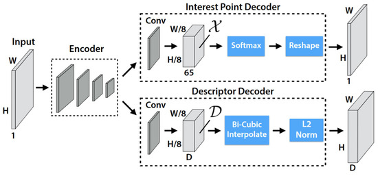
Figure 4.
SuperPoint network architecture [15].
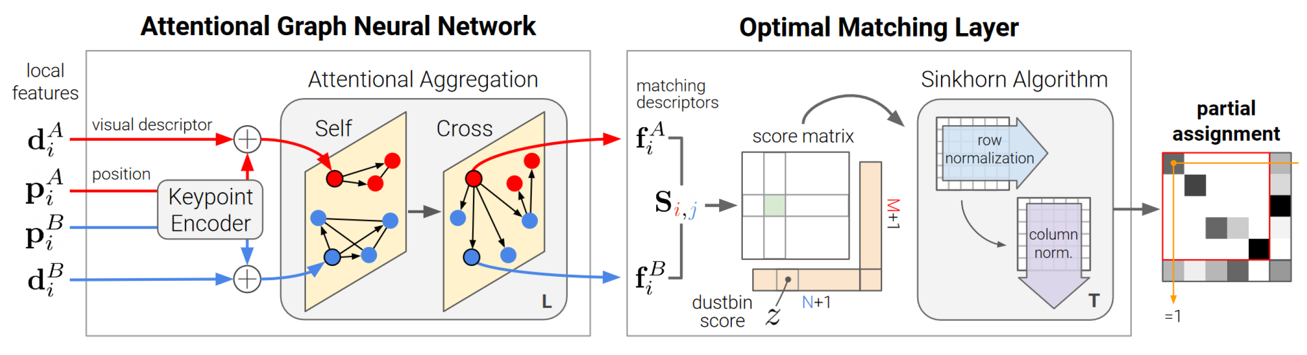
The SuperGlue Network, based on the Graph Convolutional Neural Network, matches two images’ keypoints and descriptions. The network has an Attentional Graph Neural Network and Optimal Matching Layer as shown in Figure 5.
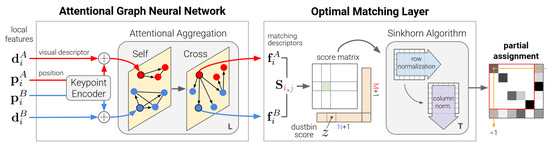
Figure 5.
SuperGlue network architecture [28].
As demonstrated in Equation (2), the former upscale keypoints using a Multilayer Perceptron (MLP) and fuses it with descriptors to create the location–appearance feature . Afterward, is regarded as a node of the graph and is inputted into a multi-layer Graph Convolutional Neural Network (GNN) to accomplish attention aggregation. The graph is composed of two types of undirected edges: intra-image edges, which connect features within the same image, and inter-image edges, which connect features between different images. Ultimately, both the self and cross-information are combined by utilizing the attention mechanism, as depicted in Equation (3). Where is the ith feature of image A in the lth layer of the graph, and denotes the attention information aggregation operation of all keypoints to i. Equation (4) shows how linear projection is used to get the aggregated feature after graph convolution for numerous layers. Equation (5) shows how the latter gets a feature similarity score S using cosine similarity based on the aggregated feature . The Sinkhorn Algorithm matches keypoints between two images based on feature similarity.
Thirdly, due to obstacles such as transformers, electrical cabinets, and fences, the tunnel segments may not be visible. This lack of effective information significantly hinders the matching of keypoints. Therefore, in the third step, it is necessary to assess the number of matched keypoints and apply specific processing to address this situation. Using the RANSAC method, we filter the keypoints that were matched above. Then, we calculate the number of matched keypoints N in the inner point set and compare it to the threshold t. When the value of N is smaller than the threshold t, it is considered to be in the occlusion state. Conversely, if N is more than or equal to t, it is not occluded. This relationship is illustrated in Equation (6). During occlusion, the accuracy of matching keypoints decreases, which can result in significant errors if not addressed. Since the camera’s movement can be considered uniform for a short period, we use the displacement of the camera in the previous unoccluded state instead of the displacement in the occluded state.
The camera motion displacement can be calculated from the displacements between adjacent image matching keypoints since the camera is moved in a fixed direction. Consider two neighboring images, where , represent the pixel coordinates of the ith feature point in image1, , represent the pixel coordinates of the ith matched keypoint in image2, n denotes the number of matched pairs, and represents the relative displacement of the current camera motion. Based on reliable keypoint matching results in the non-obscuring state, Equation (7) calculates the current camera motion displacement using the average distance of all feature point displacements.
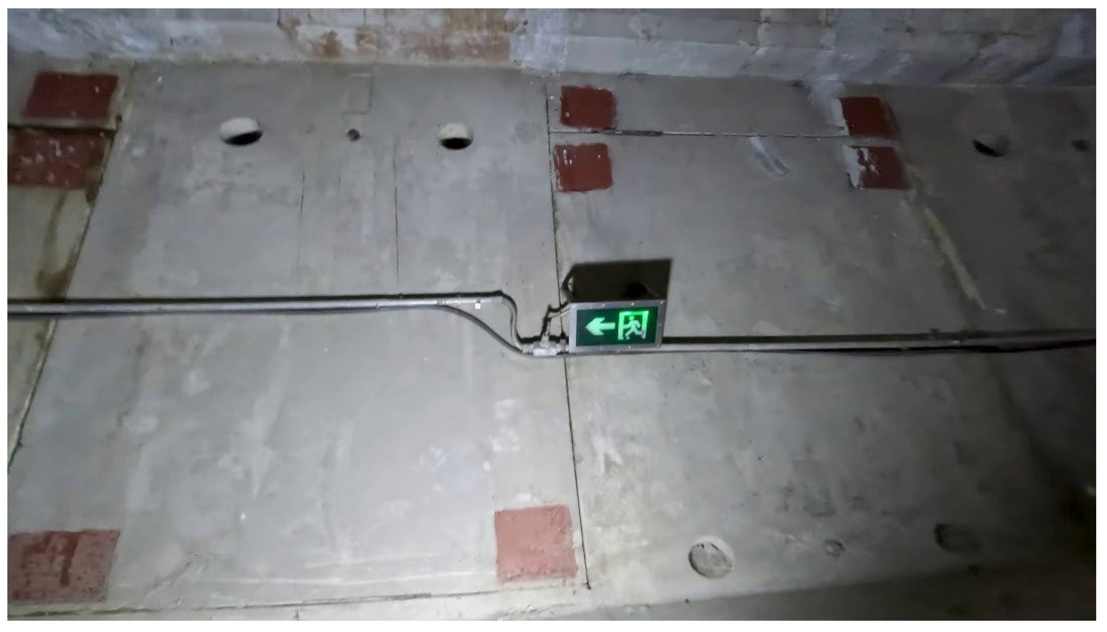
Finally, monocular cameras cannot provide an absolute scale, hence the displacements above are relative. Because visual odometry is an incremental computing process, errors accumulate at each step. Without calibration, even modest step errors will lead to massive positional errors. Thus, we calibrated the mileage using the tunnel’s evident exit signs. Figure 6 shows tunnel lining escape markers every 20 m. Based on the quantity and location of escape signs, we can calculate the actual miles and eliminate the mileage error each time an escape marker appears. Suppose there are a total of n calibration points, designated as the set , i from 1 to n, where is the sequence calibration point index and is the actual mileage at that index. To calculate the actual mileage sequence , the starting and ending miles must be known, so j from to . Equation (8) is used to calculate a scaling factor for each calibration interval to adjust the predicted mileage. For each prediction point in the interval , the calibrated mileage is , calculated as Equation (9).
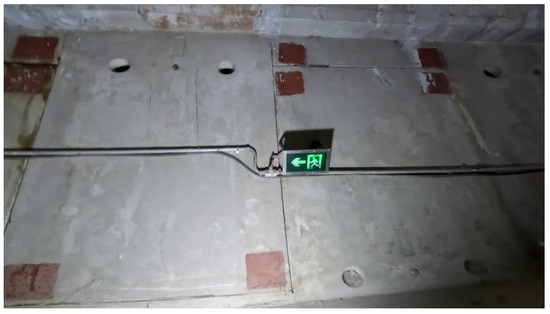
Figure 6.
Emergency route escape signs.
Through the steps above, we use the real mileage data from the calibration points to modify the predicted mileage sequence. This method can get rid of the cumulative error and provide the real mileage.
3.4. SuperPoint–SuperGlue Matching Network
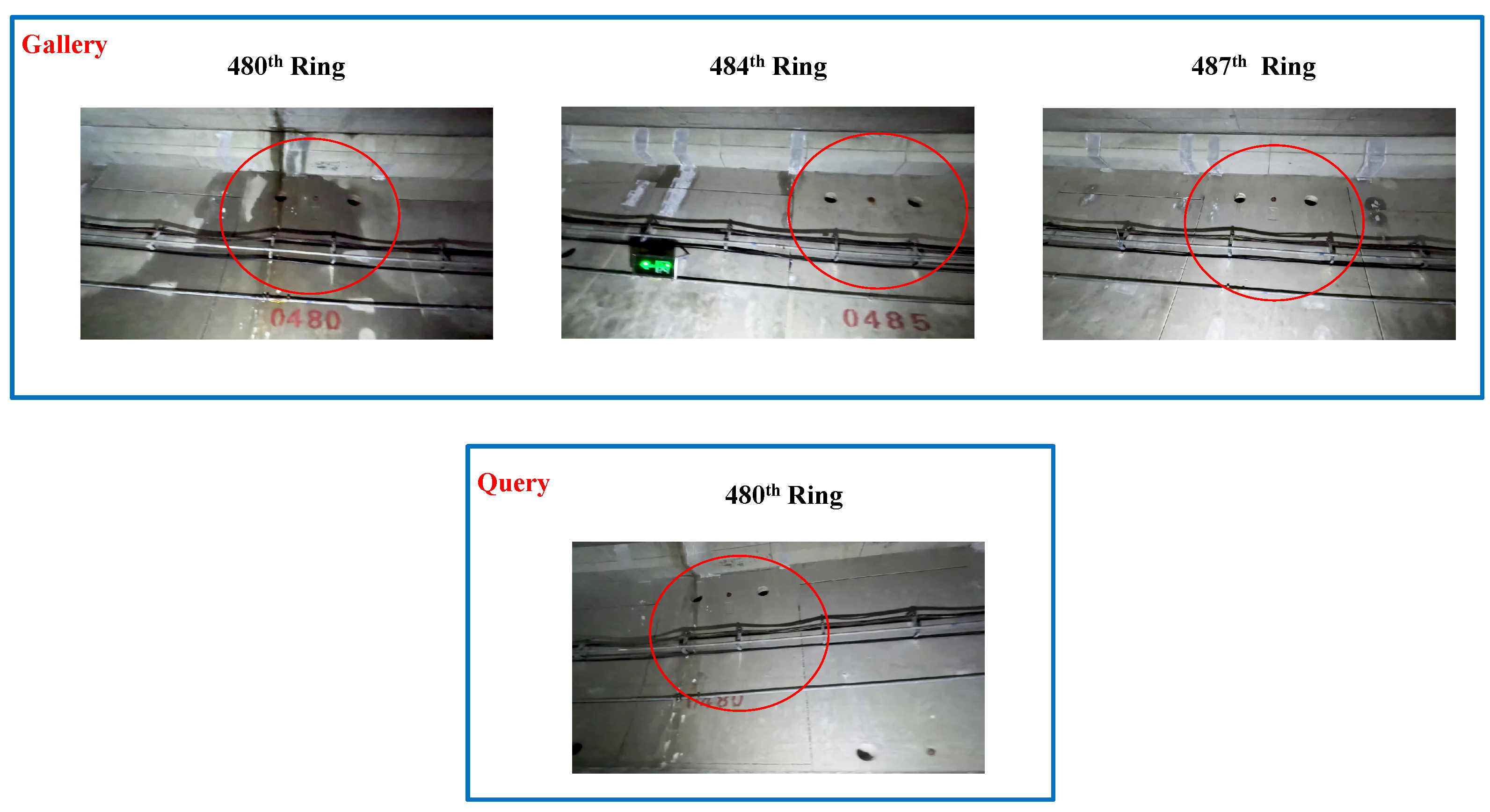
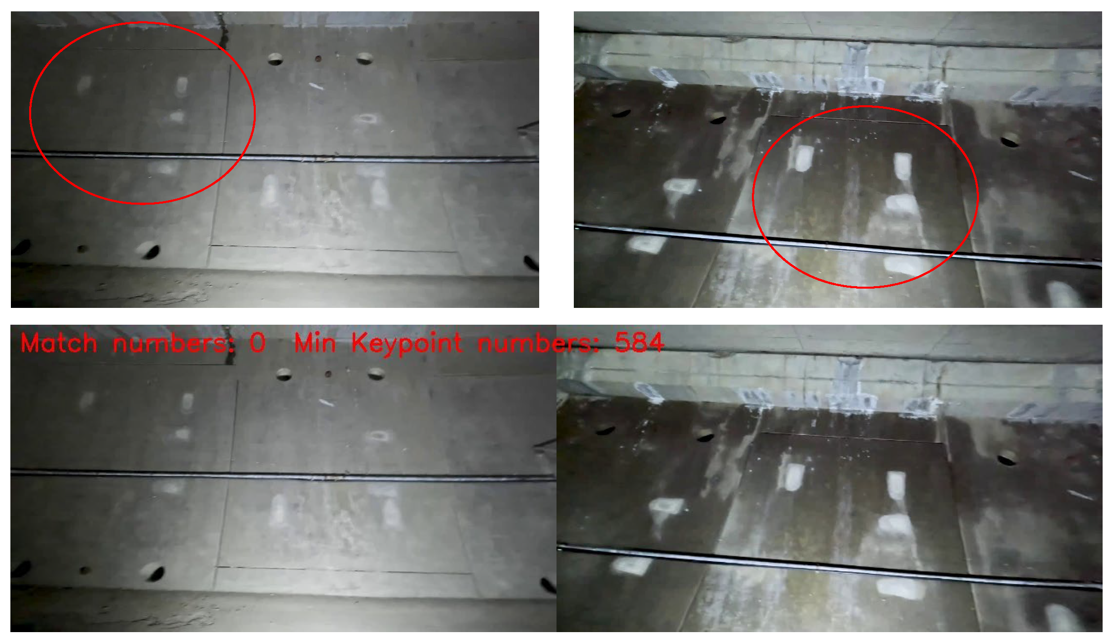
Repeated disease detection is a similarity measure task between disease images at different times. Nevertheless, the photographs of the tunnel lining exhibit a uniform texture and recurring patterns at various distances, as depicted in Figure 7. The images in the Gallery have similar structures and are similar to the disease image at the 480th ring in Query, as seen in the red circle in the figure. The efficiency and accuracy will decrease if every disease image in Query and the Gallery is compared individually using the global matching strategy. Therefore, before inputting to the SpSg Network, we split the image intervals according to the mileage information. Our location matching approach is local search. If the location of disease images in Query is p, we match the sequence in the Gallery that is within the interval , where l is a range threshold. Each disease image in Query is positionally matched with the disease image in the Gallery. All matching results are sequentially put into the network for inference.
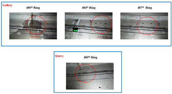
Figure 7.
Example of similar images for the Gallery and Query.
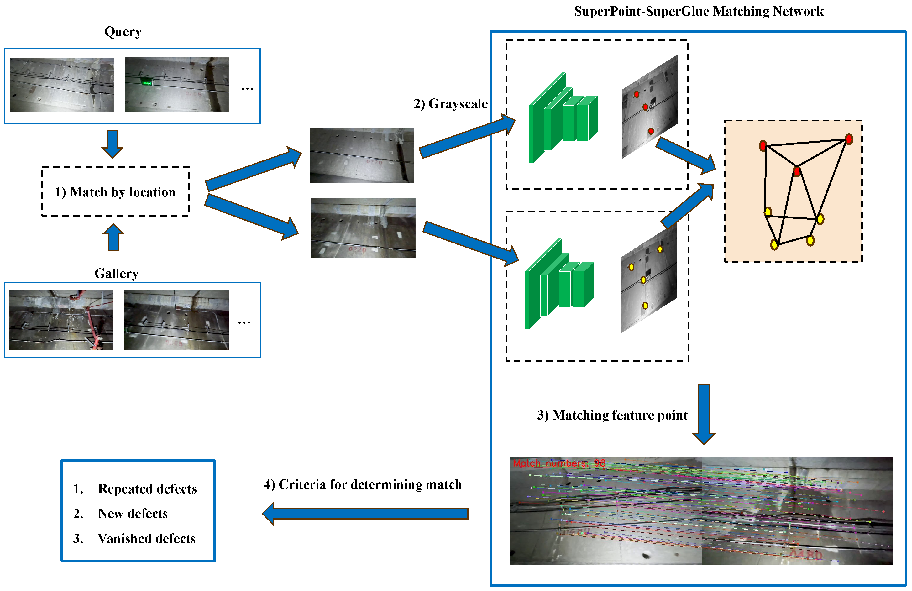
Nevertheless, it is challenging to guarantee that the camera angle, movement speed, illumination conditions, and distance to the lining surface are precisely identical for each capture. Images captured at different moments exhibit significant parallax. The existing feature point-based method, which utilizes keypoints like SIFT, SURF, and ORB, is not very effective in tunnel environments. Hence, we employ the SuperPoint and SuperGlue networks to measure the similarity of images, as depicted in Figure 8. We use the SuperPoint network to obtain the feature points and the SuperGlue network to match them. After obtaining the matched feature points between two images, we design the image matching judgment criteria. Specifically, two images are considered to be successfully matched if Equation (10) is satisfied. The variables and represent the number of keypoints in the two images. The variable represents the number of keypoints that have been matched. The judgment threshold is denoted as s, and its specific value will be determined in the experimental part using the ROC curve.

Figure 8.
Image matching process based on the SpSg Network.
We classify three different cases based on the matching results of disease images in Query (current detection results) and the Gallery (previous detection results) for the current detection results. (1) Repeated Diseases: disease images successfully matched. (2) New Disease: unmatched disease images in Query. (3) Disappeared Disease: unmatched disease images in the Gallery. Finally, the repeatability detection of tunnel diseases is finished based on inspection video data from different times.
4. Results
Our experiments are divided into three sections: an accuracy test for the Yolov7 detector; an ablation test, a comparison test, and a repeatability localization accuracy test for the SuperVO; and a comparison experiment for the Superpoint–SuperGlue Matching Network.
4.1. Yolov7 Detector Experiments
4.1.1. Tunnel Lining Disease Detection Dataset
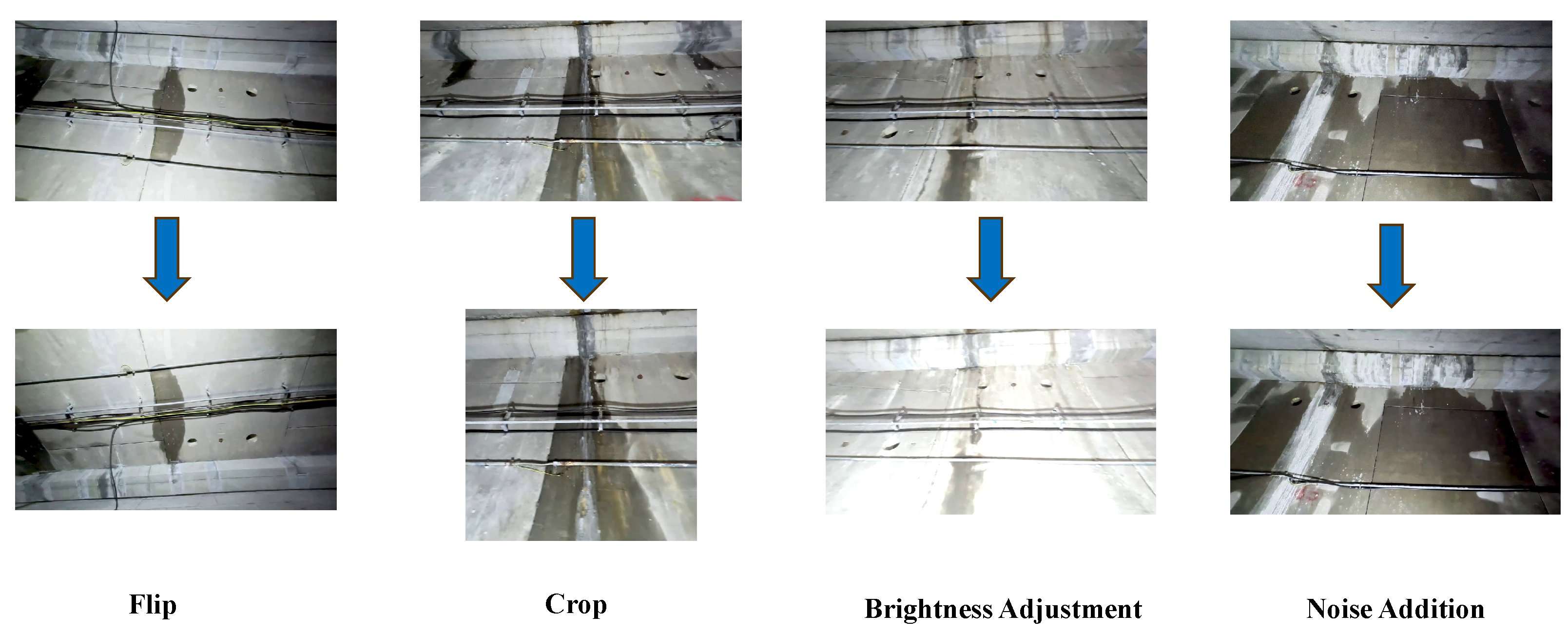
We obtained raw videos from the escape tunnel of the Yangtze River Cross Tunnel in Shanghai, which spans a total distance of 15 km. However, the current tunnel has a lower prevalence of diseases. Ultimately, we identified an overall total of 753 photos depicting leakages, which have been recorded as Dataset 1 (D1). To enhance the data, we employed various techniques such as mirror flipping, scaling, cropping, and noise addition, as illustrated in Figure 9.

Figure 9.
Example of data augmentation.
After data enhancement, a total of 2859 labeled data were obtained, noted as dataset Dataset1_Enhanced (D1E). It was also thought to add a similar leakage dataset for subway tunnels. It had 4555 sheets and was named Dataset2 (D2). Table 1 shows four combinations of the above datasets divided into training, testing, and validation sets in the ratio 6:2:2.

Table 1.
Details of disease detection dataset.
4.1.2. Evaluation Metrics and Results
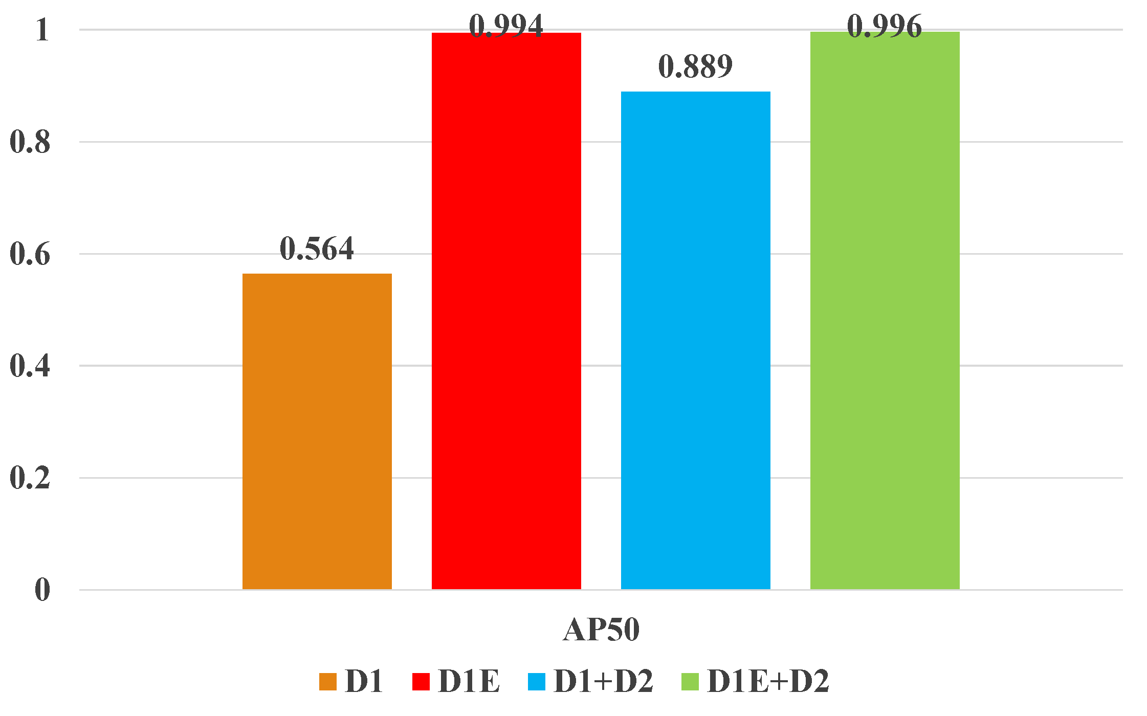
AP (Average Precision) was used to evaluate Yolov7’s detection performance, and the equation is as follows, where P is the precision and R is the recall. PR is a curve with recall R on the horizontal axis and precision P on the vertical, and AP is its area. TP and FN are related to IoU (Intersection over Union), and AP is called AP50 when IoU is 0.5. We used the same experimental setup and hardware for 200 epochs to test the weights trained on different datasets on the D1 test set. The final experimental findings are presented in Figure 10.

Figure 10.
Results for different combinations of datasets.
Experimental results show that D1 is not enough to train a more general detector. However, data augmentation improves D1E detection accuracy to 99.4%, which is sufficient for tunnel disease detection. After adding the subway leaking dataset (D1+D2), detection accuracy also improved, however, it was lower than the data augmentation, mostly because the Cross-River Tunnel and subway tunnel scenarios have different leaking image characteristics and data distribution. Finally, we chose D1E+D2 dataset weights.
4.2. SuperVO Experiments
4.2.1. Datasets and Evaluation Metrics
We recorded the escape tunnel lining video twice at separate times and chose Video1 of the tube sheet without obstruction and Video2 with obstruction in the first data collection. Video3, with the same mileage as Video1, was selected for the second data collection. The frames were extracted at the same interval for all three videos. Table 2 shows the dataset details. The mean error and maximum error were used to evaluate the visual odometer’s accuracy. The calculation equations are (14) and (15), respectively, where N is the number of marker points, is the kth marker point’s estimated value, and is its real value. These criteria assess the odometer’s robustness and maximum deviation.
Table 2.
Visual odometer dataset.
4.2.2. Optimal Threshold t Determination
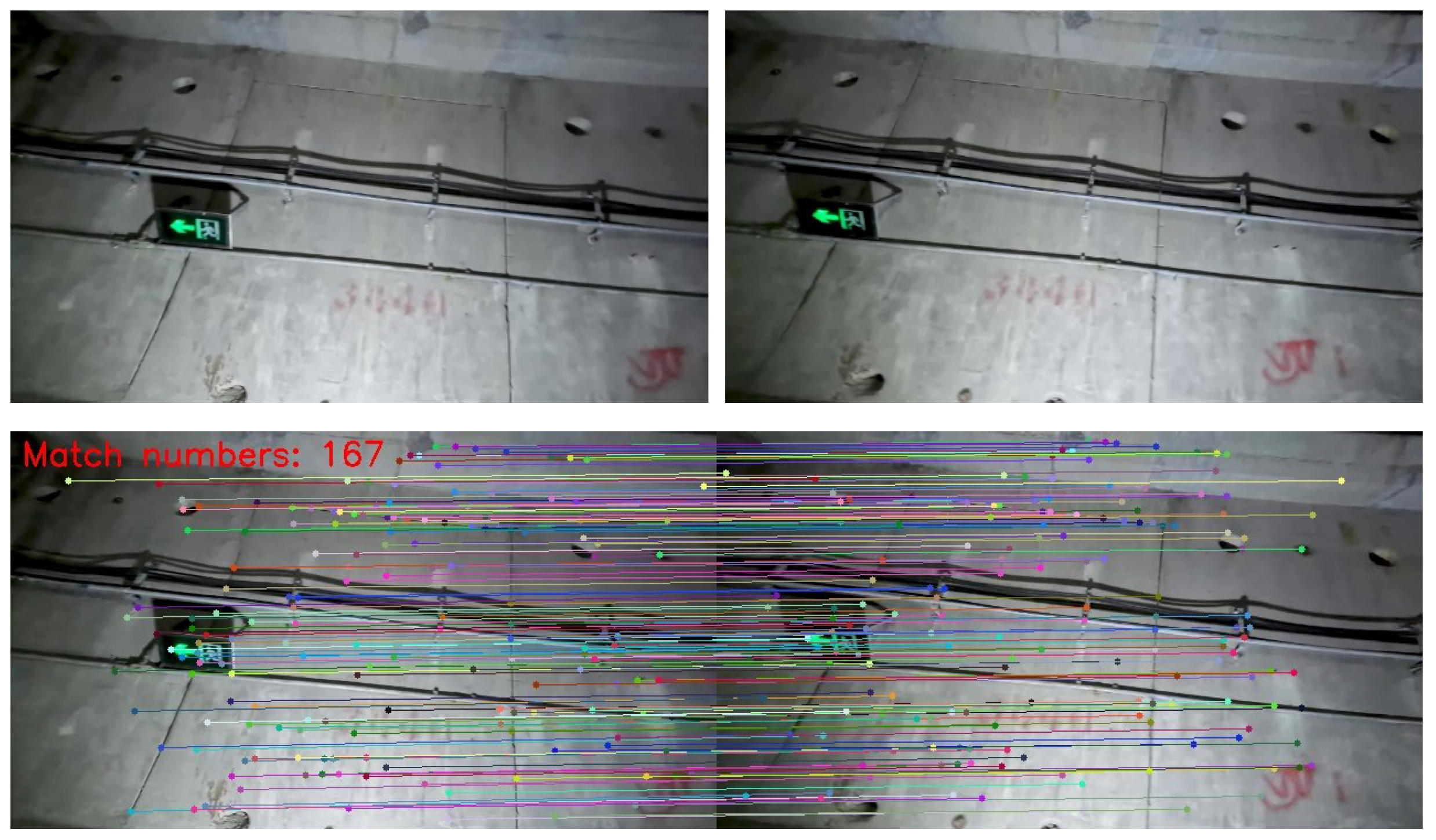
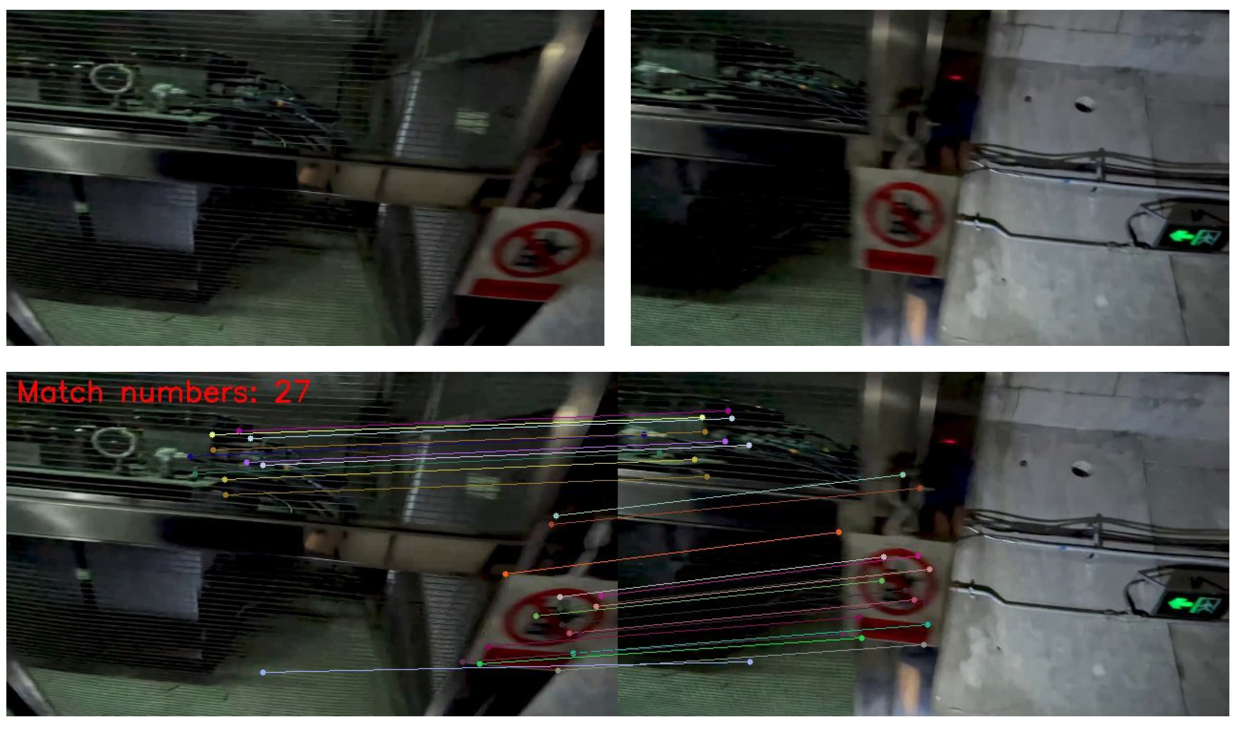
The tube sheet is obscured by transformers, electrical cabinets, fences, etc. in actual tunnels, which severely reduces the number of successfully matched image keypoints. Figure 11 and Figure 12 show keypoints matching for non-obscuring and occluding. The difference in matching keypoints between non-obscuring and obscuring is significant, with the former having 167 points and the latter only 27. Thus, these two states require identification and separate processing.
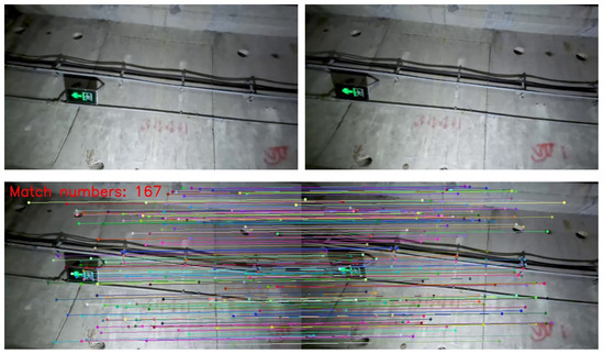
Figure 11.
Results of matching feature points without occlusion.
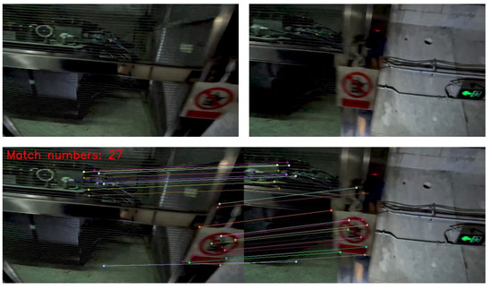
Figure 12.
Results of matching feature points with occlusion.
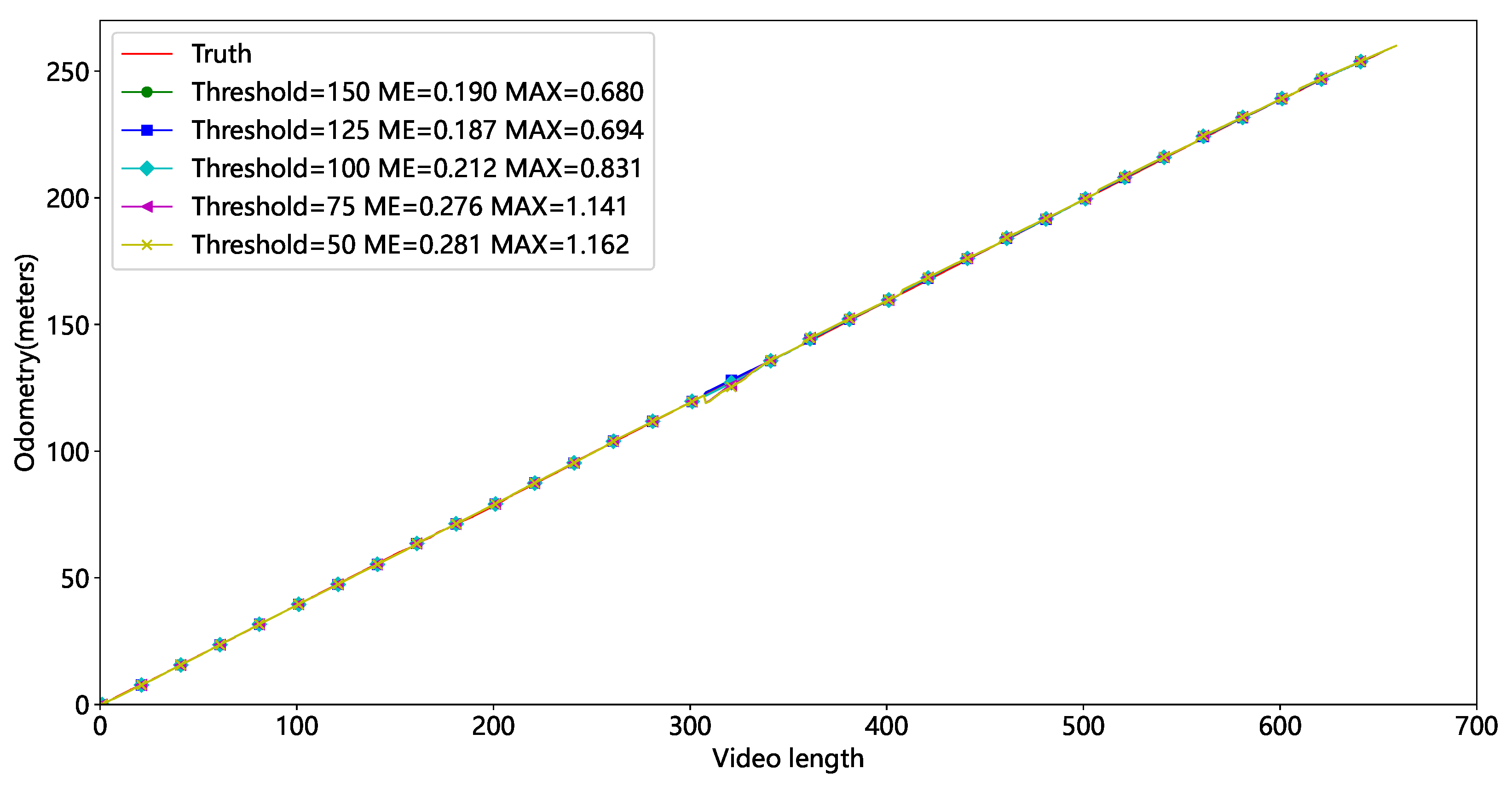
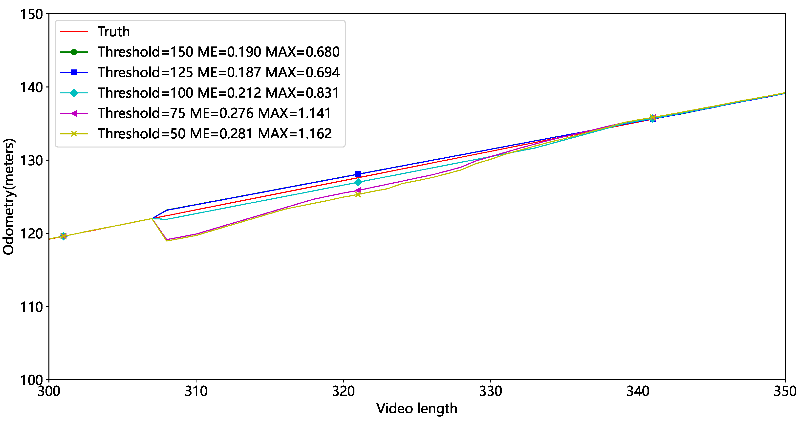
In Video2, the experiment is run with different thresholds t, and the results are presented in Figure 13 and Table 3. Red represents the actual mileage, while other colors represent mileage at differing thresholds. Figure 13 shows some mileage deviation around 300 frames due to the tube sheet being occluded. Figure 14 shows that the mileage error is relatively large at thresholds of 75 and 50, indicating that fewer feature points result in larger inaccuracies. We set t at 125 based on average and maximum errors.
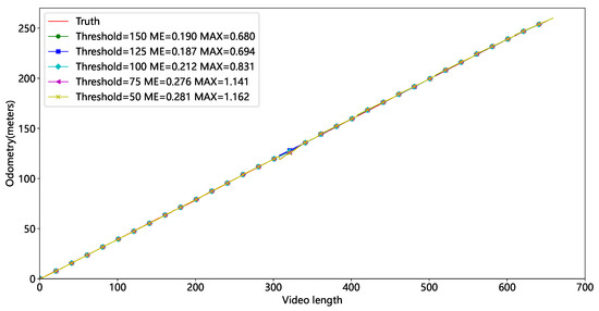
Figure 13.
Mileage results at different thresholds.
Table 3.
Results of different thresholds t.
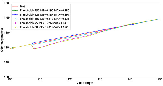
Figure 14.
Local mileage results at different thresholds.
4.2.3. Ablation Experiment
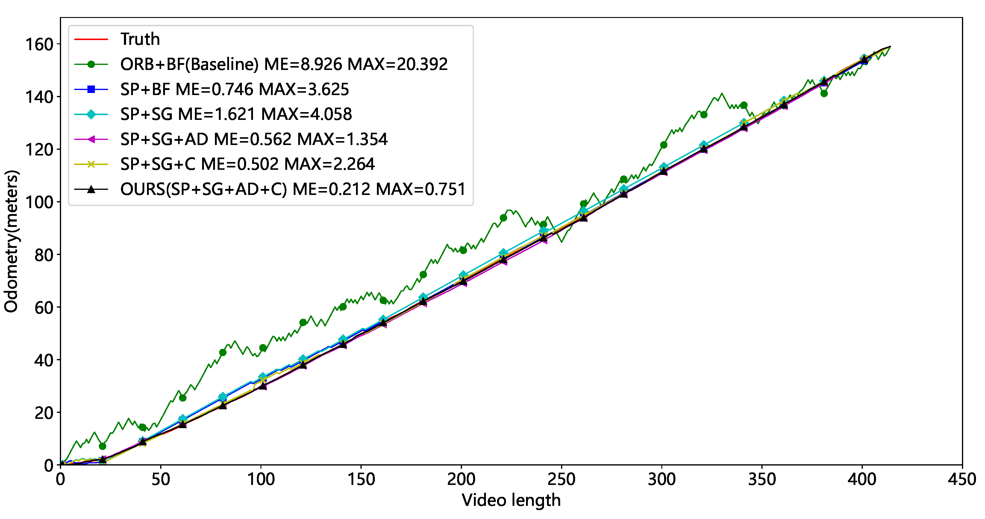
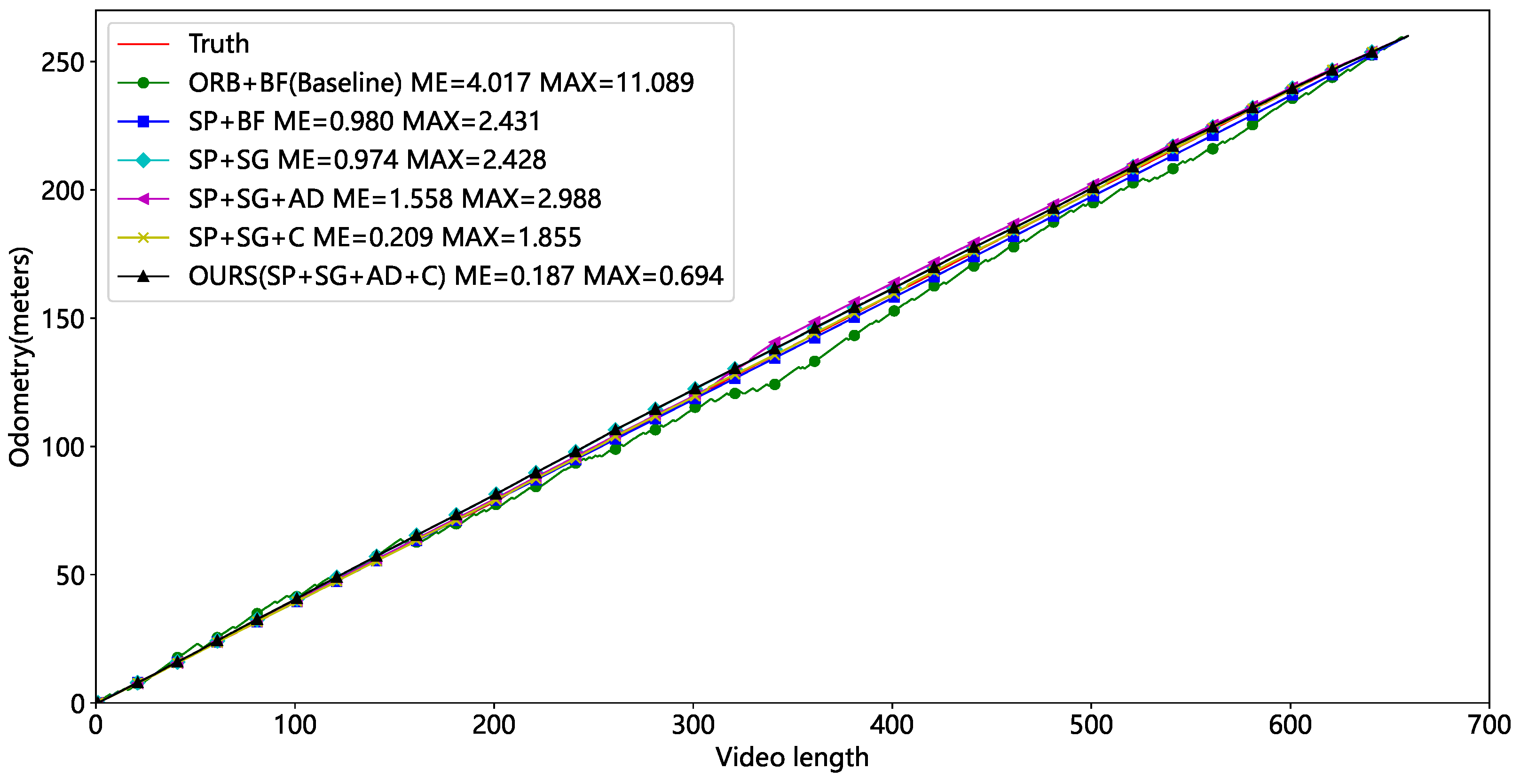
After finding the appropriate threshold, we performed ablation tests on Video1 and Video2, (1) using ORB keypoints, a brute-force matching strategy, and the polar line constraints denoted as ORB+BF, which is the Baseline for our comparison. (2) Using the SuperPoint, a brute-force matching strategy, and the polar line constraints denoted as SP+BF. (3) Using the SuperPoint, the SuperGlue, and the polar line constraints, denoted as SP+SG. (4) Using the SuperPoint, the SuperGlue, and the average displacement of the matched keypoints, denoted as SP+SG+AD. (5) Using the SuperPoint, the SuperGlue, the polar line constraints, and calibration denoted as SP+SG+C. (6) Using the SuperPoint, the SuperGlue, the average displacement of the matched keypoints, and marker point calibration denoted as SP+SG+AD+C, and this method is our final solution.
Table 4 and Table 5 show the Video1 and Video2 test results for the six combinations. Our approaches have the lowest average and maximum errors and outperform the Baseline. The mileage curves of different approaches are presented in Figure 15 and Figure 16. ORB feature points have the worst performance and huge fluctuations, making them unsuitable for tunnel applications. The SP+BF method outperforms Baseline, showing that SuperPoint can generalize even in tunnel circumstances with sparse and repeating textures.
Table 4.
Results of the ablation test without occlusion.
Table 5.
Results of the ablation test with occlusion.
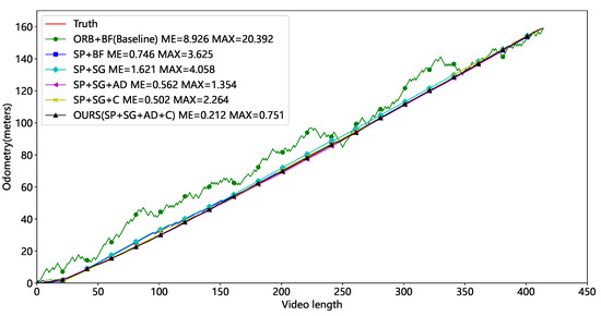
Figure 15.
Comparison of mileage for different methods (without occlusion).
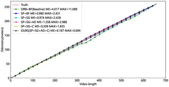
Figure 16.
Comparison of mileage for different methods (with occlusion).
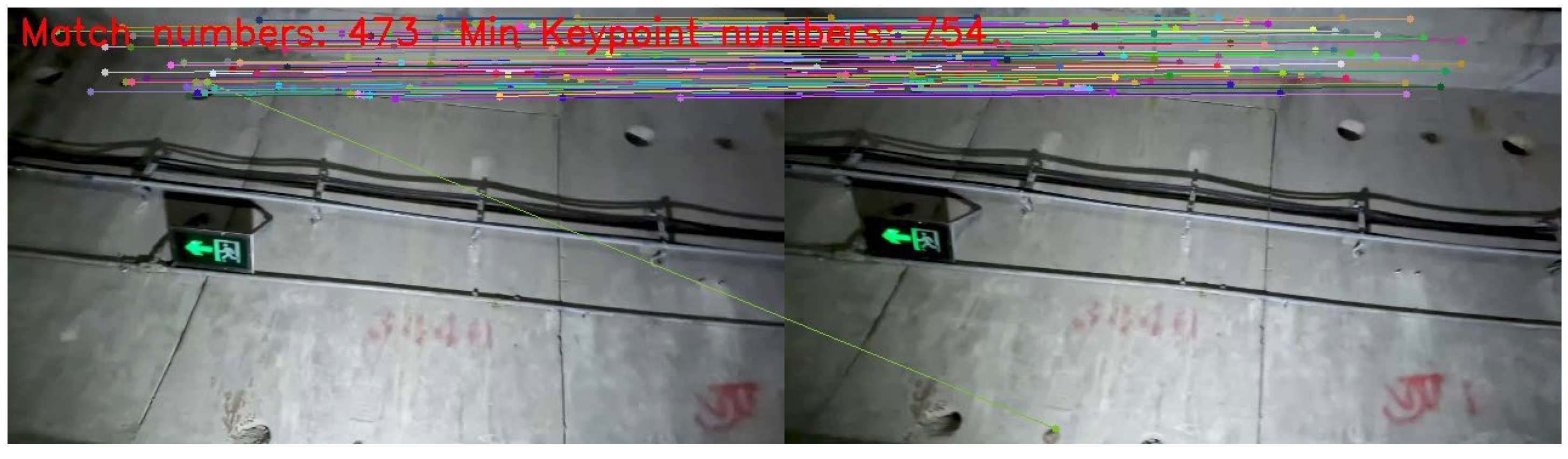
The primary distinction between the SP+SG and SP+BF is the matching technique. The SuperGlue can match a greater number of keypoint as illustrated in Figure 17 and Figure 18. There is an obvious mistake in the brute-force matching. Nevertheless, the precision of the mileage performed by SP+SG on Video1 is worse compared to SP+BF, possibly as a result of incorrect matching and the failure to eliminate errors. While SuperGlue can yield a greater number of match points and more precise matches, it is still possible for mismatches to happen. Even a small number of these false matches might have a substantial impact on the final pose estimation. Consequently, in the next procedure, we employed the RANSAC algorithm to exclude the mismatched keypoints.
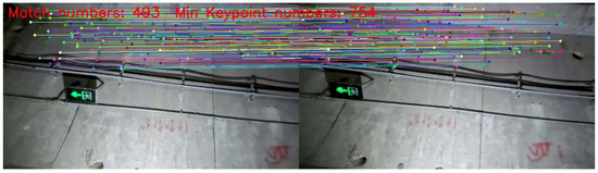
Figure 17.
SuperGlue network matching results without occlusion.

Figure 18.
Brute-force matching results without occlusion.
The primary distinction between the SP+SG+AD and the SP+SG lies in the approach used to calculate camera displacement and the utilization of the RANSAC algorithm. It is evident that in the absence of occlusion, utilizing the average displacement for calculating camera displacement can effectively decrease both the average and maximum errors. However, in the presence of occlusion, the error of this method slightly increases. This demonstrates that the quantity of accurately matched keypoints is a crucial factor. After calibration, the final method is within 0.3 m of the mean error and 0.8 m of the maximum error. This highlights the need to eliminate cumulative errors in visual odometry. Our approach allows precise localization of a scene that lacks texture using a monocular camera.
4.2.4. Comparative Experiment
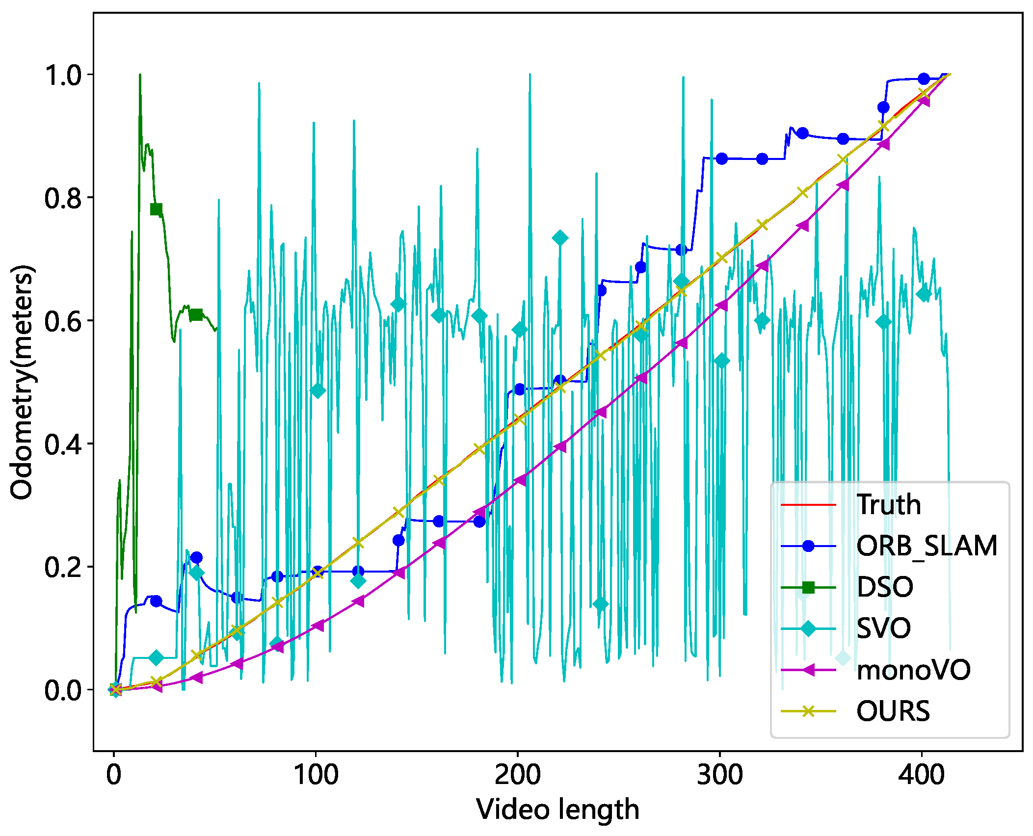
The comparison algorithms include ORB-SLAM [31], Lucas–Kanade optical flow-based monocular odometry (monoVO), Semi-Direct Visual Odometry (SVO) [32], and Direct Sparse Odometry (DSO) [33]. The results were evaluated in both unobscured and occluded scenarios, as depicted in Figure 19 and Figure 20.
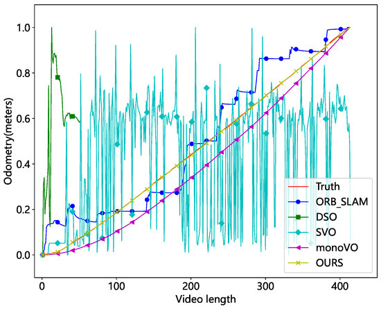
Figure 19.
Comparison of different methods without occlusion (normalized mileage).
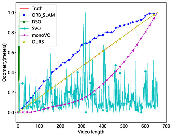
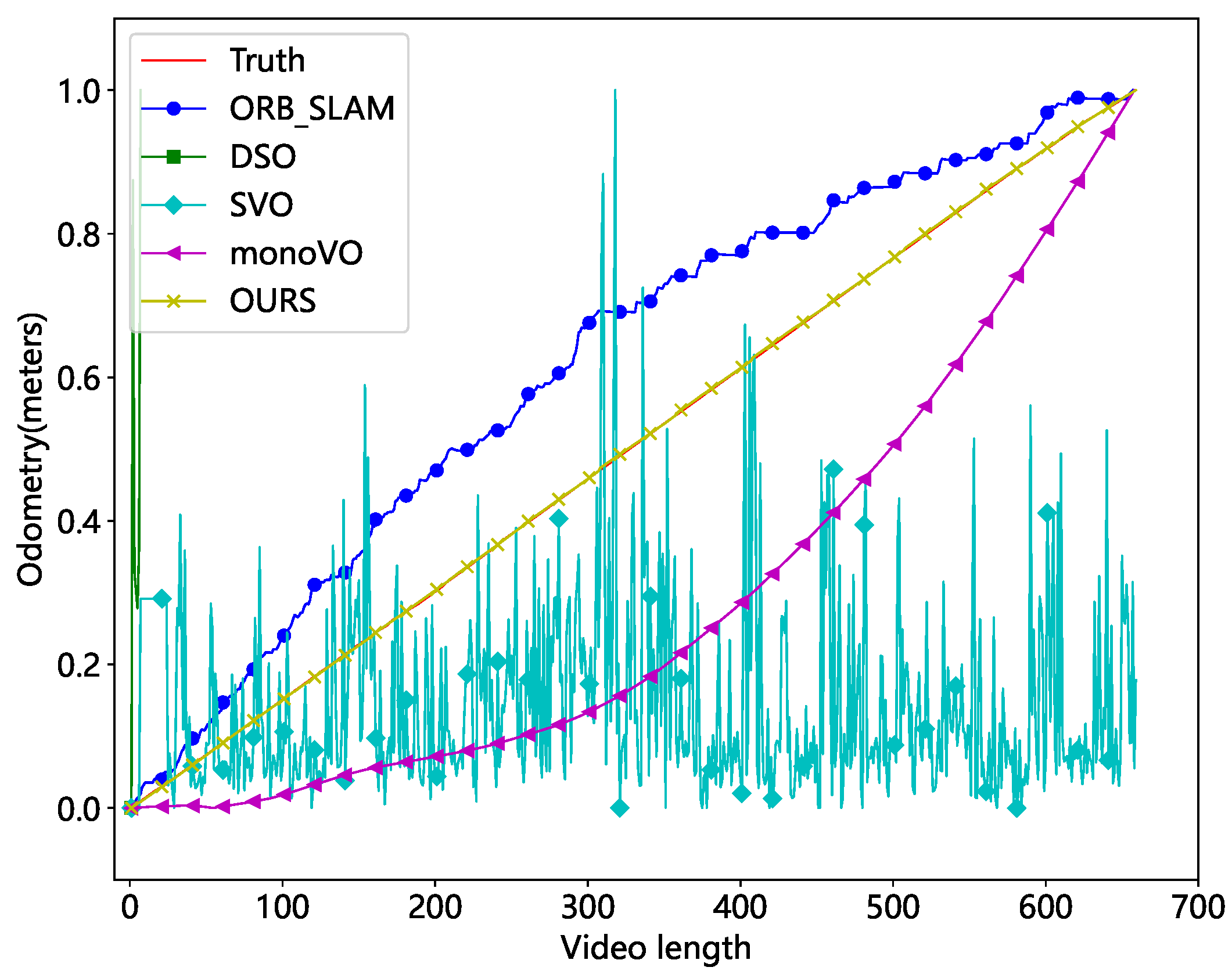
Figure 20.
Comparison of different methods with occlusion (normalized mileage).
The results demonstrate that the DSO and SVO methods are the least effective. DSO is a direct method that identifies pixel points with obvious gradient texture features. However, the real test demonstrates that the photometric features are centered on the cables, making it impossible to match the walls. SVO is a semi-direct approach that combines the direct and feature point methods. It obtains the camera posture by directly matching the feature point image blocks. However, this method is unable to eliminate the cumulative error. The keypoints employed are particularly susceptible to loss in tunnel environments, and the odometer will be reset frequently. So, the entire odometry curve has an oscillating shape. ORB-SLAM is a monocular SLAM system that uses Oriented FAST and rotated BRIEF (ORB) as the fundamental feature. When the current frame cannot be matched with the nearest neighbor keyframes, it uses a relocation mechanism to match all keyframes. Because ORB features are frequently lost in tunnel images, the method’s overall distance profile seems stepped. The monoVO tracks the motion of keypoints using Lucas–Kanade optical flow, reducing feature point matching loss. As a result, the approach performs better but still exhibits significant localization errors. Our method is a type of monocular visual odometry that uses sparse keypoints. By using SuperPoint and eliminating cumulative error, it achieves great localization performance even in challenging tunnel circumstances.
4.2.5. Repeatable Localization Accuracy Test
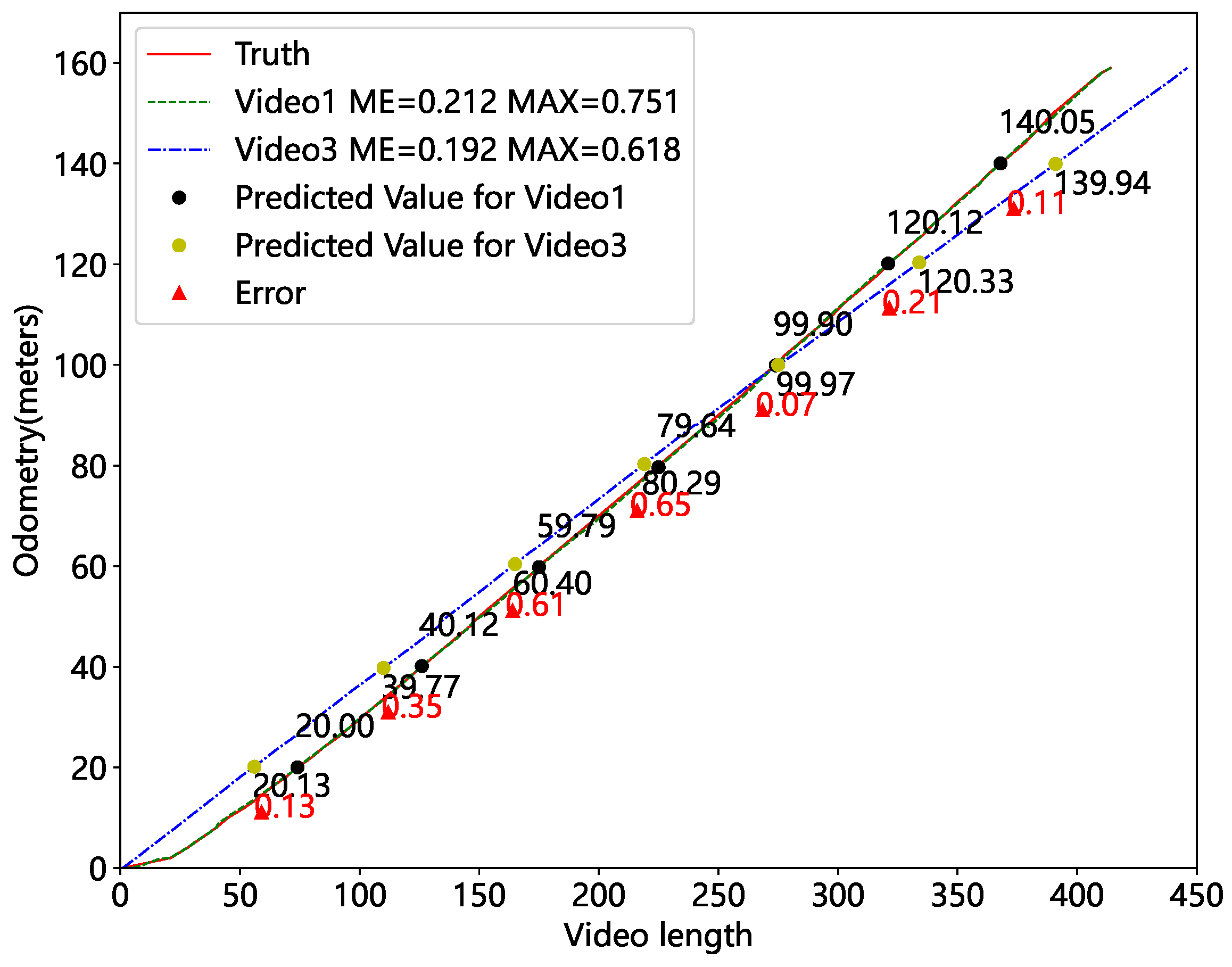
To further verify that the localization algorithm can perform repetitive localization, we chose to examine two videos recorded at different times in the same location, Video1 and Video3. Figure 21 shows the mileage estimation results. We selected seven marker points with real mileage for comparison, and the red triangles represent the error between the two predictions. The specific data are presented in Table 6. The largest discrepancy between the two mileage predictions is 0.65 m. Meanwhile, the difference between the two mileage predictions and the true value is within 0.4 m. It validates the accuracy of our method’s repetitive localization. Therefore, it can divide the image into distinct sections depending on mileage and feed accurate inputs to the image matching network.

Figure 21.
Mileage estimates for videos from different periods.
Table 6.
Results of repeatability localization.
4.3. SuperPoint–SuperGlue Matching Network Experiments
4.3.1. Datasets and Evaluation Metrics
We recorded a video of the escape tunnel’s lining twice. After detection and localization, 556 images from the initial inspection video were retrieved and combined to form a Gallery. Due to tunnel disease repair, only 89 disease images were collected in the second collection, creating a Query. The final image matching test data were created with Query and a Gallery. The illumination conditions, shooting angles, and acquisition directions were all different in both cases. Figure 22 shows that even images from the same position have a large parallax. The Siamese structures employed for image matching are trained on generalized datasets that differ significantly from our specific scenario. Therefore, it is necessary to create a customized dataset for fine-tuning these networks. The dataset consists of 4000 images divided into 100 classes, with each class representing images acquired at different mileages.
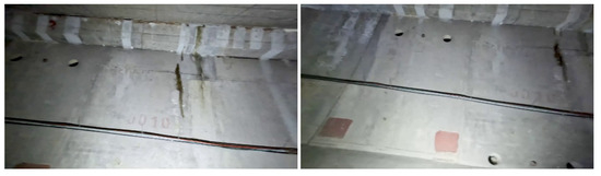
Figure 22.
Disease images at the same location in Query and the Gallery.
Our task is to assess disease image pairs, which can be thought of as a binary classification problem. We utilized the receiver operating characteristic curve (ROC curve) to compare results. In our situation, identifying whether two diseases have the same ID can be considered a dichotomous problem, with samples classified as positive (i.e., samples of diseases with the same ID) or negative (i.e., samples of diseases that do not have the same ID). When predictions are made, four cases occur: (1) the instance is ID1 and the prediction is ID1, i.e., TP (True Positive); (2) the instance is ID1 and the prediction is ID2, or the instance is in the negative class and the prediction is in the positive class, i.e., FP (False Positive); (3) the instance is in the negative class and the prediction is in the negative class, i.e., TN (True Negative); and (4) the instance is in the positive class and the prediction is in the negative class, i.e., FN (False Negative). This gives us the definitions of TPR and FPR.
For different classification thresholds, a point can be created by using TPR and FPR as horizontal and vertical coordinates. Modify the thresholds and re-compare them, then link all of the results to form a single curve, known as the ROC curve. The area under the curve, called the AUC, is employed as an evaluation criterion in the ROC curve. Closer to 1 indicates stronger recognition ability, whereas closer to 0.5 indicates poorer recognition ability. The ROC curve also allows us to calculate the best classification threshold, which is the value at which the difference between TPR and FPR is greatest. In addition to the ROC curve, we employ the average query time, precision, recall, and F1 score as evaluation metrics, which are described in the equation below.
4.3.2. Optimal Threshold l Determination
Before using the SpSg Network, we separated the image into several intervals based on the odometer value. The disease image’s location in Query is p, and the images that need to be matched are the sequences in the Gallery whose locations fall within the interval . Consider that the view of a single image has three rings of pipe information. Even with accurate odometer localization, severe circumstances like the same disease appearing on the left side of the image for the first time and on the right for the second time would result in a three-ring positional gap. Thus, we chose thresholds from three rings and incremented by one ring for each test. Detailed results are in Table 7. The ultimate threshold value is 5 after considering P, R, and F1 score.
Table 7.
Results of different thresholds l.
4.3.3. Comparative Experiment
We compared two image matching methods: one uses local feature points and the other uses depth features. The former includes (1) ORB+BF, which uses ORB and brute-force matching. (2) SP+BF uses SuperPoint and brute-force matching. Our method leverages the SuperPoint and SuperGlue network, also from this category. These two methods can be employed for ablation tests.
The second category involves implementing image matching using deep features. It extracts deep characteristics from widely used backbone networks and estimates image similarity using a Siamese structure. The backbone networks employed are (1) VGG [34], (2) DarkNet53 [35], (3) EfficientNet [36], (4) ResNet [37], and (5) Res2net [38]. The dataset created in the previous part was used for training. Because of the tiny amount of data, we employed a transfer learning strategy. During training, the backbone network employed weights that were previously trained on the IMAGNET dataset. We trained the network for 100 epochs with the Adam optimizer and an initial learning rate lr of 0.0001, then decreased the learning rate using StepLR at equal intervals. Due to hardware constraints, the image size was set at 640 × 640 and the batch size to 4. We used the CentOS 7 operating system and the Tesla T4-16 GB GPU produced by NVIDIA in Santa Clara, CA, USA.
Table 8 shows the experimental results for different methods. The ORB+BF approach produces the worst results due to the tunnel’s lack of texture and repeating features. The SP+BF approach has improved accuracy since the introduction of SuperPoint. However, because the image has a significant parallax and fewer overlapping regions, the BF method often results in incorrect matches. Our approach employs a SuperGlue network that combines feature point localization and appearance information. Additionally, we utilized an Attentional Graph Neural Network that facilitates communication between features inside an individual image and across multiple images. Our approach had a precision of 96.61%, a recall of 93.44%, and an F1 score of 95%.
Table 8.
Image matching comparison test results.
All the strategies for matching based on depth features were ineffective. The tunnel images shared a similar overall structure and texture. And, depth features are difficult to distinguish, hence it is preferable to employ local feature points for discrimination. In addition, the VGG* was the least successful since it does not freeze the weights of the backbone network throughout training. It also showed that transfer learning is a successful method. In terms of speed, the deep feature-based method extracted the features of the entire image for comparison, which is faster. A single image’s matching time was up up to 0.14 s. However, our approach extracted and matched all of the images’ feature points. As a result, it took 4.80 s to match a single image. The main issue for our repetitiveness detection task is whether it could correctly match diseases in the same region. Since our method was able to achieve good image matching, it can be used for the constant detection of tunnel degradation in real tunnels.
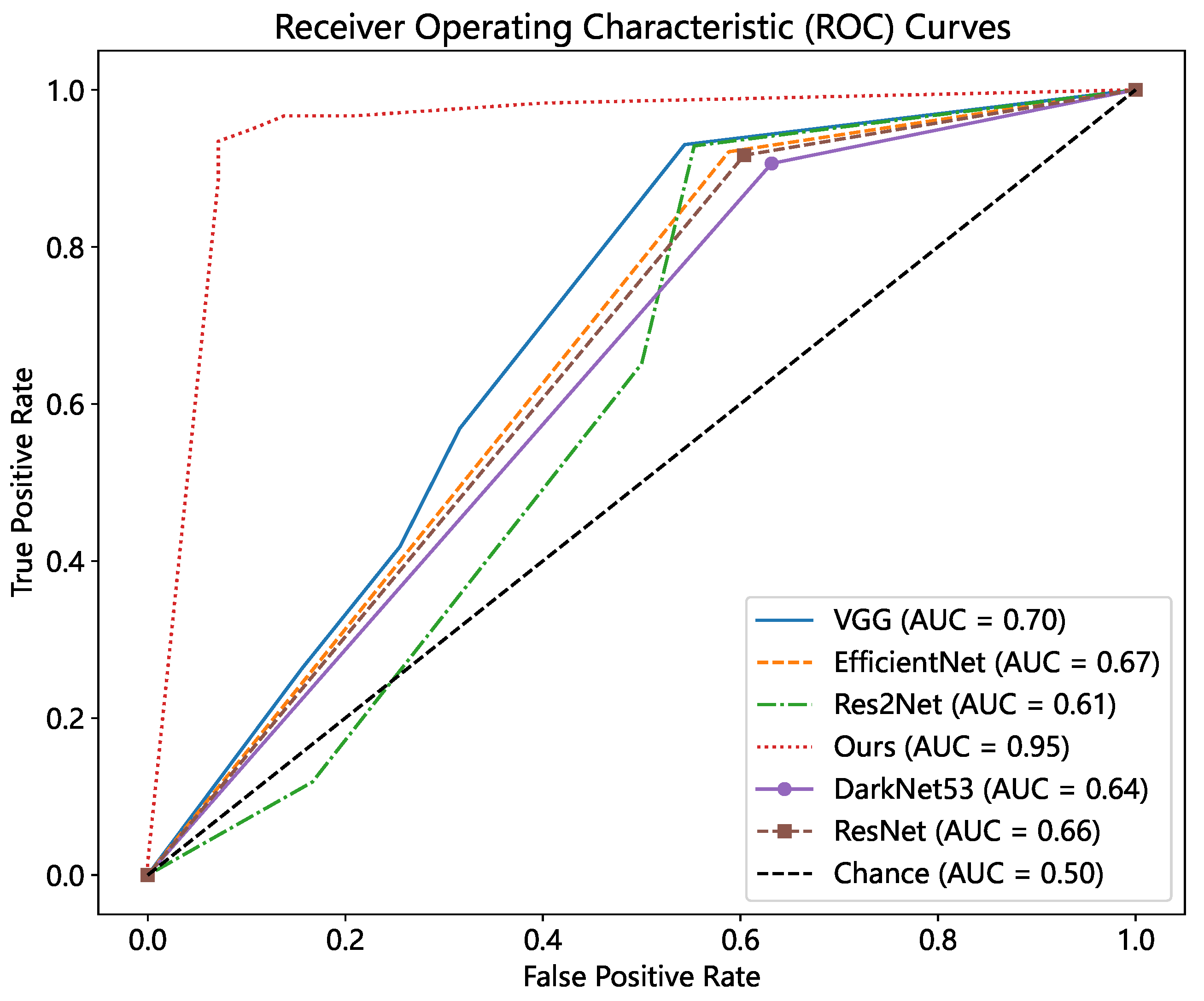
To compare our method’s classification ability, we plotted ROC curves for all of the models by adjusting the thresholds, as shown in Figure 23. The threshold value s of our method ranged from 0 to 1. We drew the ROC curve with different thresholds s at an interval of 0.1, and determined the optimal threshold s according to the Youden index. We know that our method produces the best results, with an AUC of 0.95 and an optimum threshold s of 0.3. VGG had the second-best results, with an AUC value of 0.7, but deeper networks such as ResNet and Res2Net performed poorly. It also demonstrates that using deep characteristics to match images should be avoided when the image structure and texture are similar.
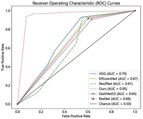
Figure 23.
ROC curve comparison.
4.3.4. Defect Repeatability Detection Results
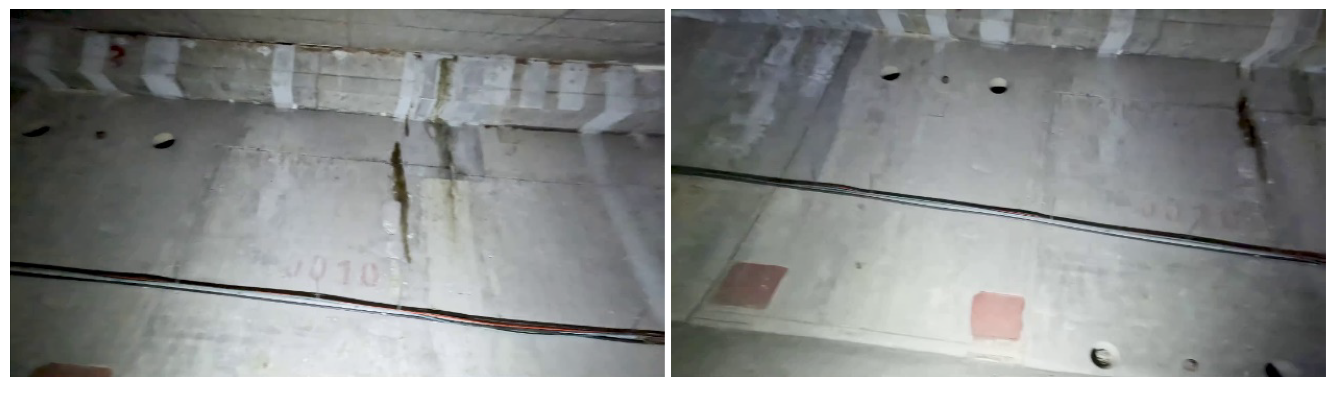
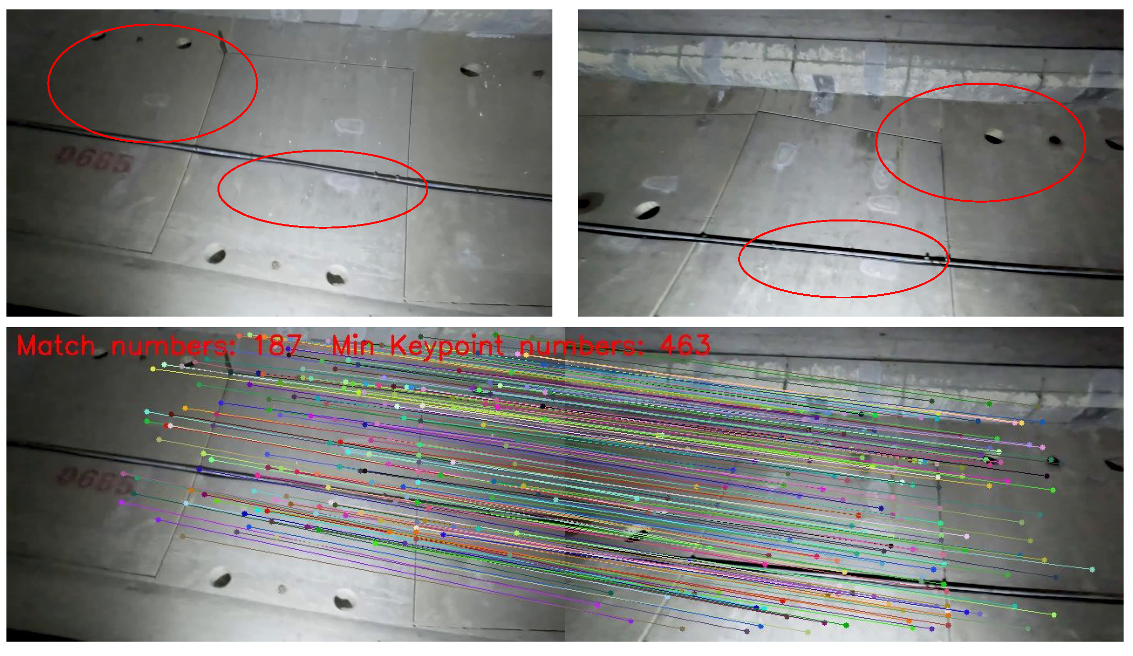
Finally, the repeated detection results of Query and Gallery matching were calculated. Table 9 shows the number of repeated, new, and vanished diseases. Among those predicted new diseases, 26 were correct and 4 were wrong. A total of 57 of the predictions for repeated diseases were true, while 2 were incorrect. In comparison to the actual situation, 3 repeated diseases and 3 new diseases were not predicted. Figure 24 and Figure 25 demonstrate examples of incorrect and missed matches, respectively.
Table 9.
Comparison of repeatability detection results.

Figure 24.
Example of incorrectly matched images.

Figure 25.
Example of missing match images.
The image example on the left side shows the image in the Query with a distance of 686 m, whereas the image on the right side shows the image in the Gallery with a distance of 684.72 m. The number of properly matched feature points was 187, which were concentrated in the red zones as depicted in Figure 24. These regions shared similar image structure and texture, with cables, seams, mounting holes, and repair markings.
The image on the left side of the missing matching example is from the Query, with a distance of 282.91 m. The image on the right side is from the Gallery, with a distance of 282.54 m. These two images may be determined to be at the same location based on the red area in the figure and the distance information. However, the presence of parallax and changes in diseases prevented the successful matching of any feature points. For this extreme case, a feasible approach is to match based on mileage information only. Despite a few missing and incorrect matches, the overall number of errors was minimal. The majority of them could be accurately recognized. The precision reached 96.61%, and the recall was 93.44%. It offered an effective solution to the problem of repeating detection in real tunnels.
5. Conclusions
To address the lack of disease dynamic change monitoring in current tunnel lining surface disease detection methods, this paper proposes a disease repeatability detection method based on multi-information fusion. The method firstly utilizes Yolov7 to obtain the location information of the disease in the image; then, the SuperVO algorithm is designed for obtaining the actual mileage information of the disease; subsequently, the SpSg image matching network is designed for obtaining the similarity information of the disease images. Finally, the above information is fused to realize the repetitive detection of tunnel diseases. This enables tunnel maintenance personnel to accurately assess disease trends and better formulate maintenance measures. It improves the science and accuracy of tunnel maintenance decisions.
Conventional visual odometry methods fail to localize tunnel lining images due to their limited and repetitive texture information. Thus, we present SuperVO, which accurately matches tunnel image features. The method can accurately obtain actual mileage information for tunnel diseases by using the SuperPoint network, the SuperGlue network, and actual mileage calibration. The results demonstrate that our proposed strategy is more effective. In two actual tunnels with lengths of 159 m and 260 m, the average localization error is less than 0.3 m, and the maximum error is less than 0.8 m.
On the other hand, identifying the disease’s development trend requires image matching. Current feature point-based image matching algorithms perform poorly in tunnel scenarios with high structural similarity. Deep learning-based image matching approaches require a huge number of data labels, and since images taken at different locations are too similar, the depth features are difficult to distinguish. Therefore, we initially utilize the mileage information to perform a coarse matching. Then, we present the SpSg Network, which uses the SuperPoint and the graph neural network SuperGlue to accomplish the fine matching. The results demonstrate that the framework achieves 96.61% precision, 93.44% recall, and a 95% F1 score in real tunnels. It demonstrates the practical value of the proposed method.
In the future, the following research directions still need to be explored and optimized in depth. (1) Due to the limitations of the dataset, this paper focuses on the repetitive detection of leakage diseases. Future work needs to more extensively collect and analyze different kinds of tunnel disease data. By increasing the diversity of the dataset, the adaptability of the model to complex disease scenarios can be improved. It also significantly enhances the generalization ability of the model. (2) To improve tunnel localization accuracy and reduce dependence on marker points, Binocular cameras can be utilized to accurately determine the location of the disease. By analyzing the parallax of pixels captured by the cameras from two different viewpoints, the depth information of each point in the image is accurately calculated. Thus, the precise location of the disease in three-dimensional space can be realized. (3) Meanwhile, we will attempt to utilize image segmentation technology to achieve repetitive measurement by aligning the matched images to complete the quantitative analysis of disease development. (4) Finally, we will create an intelligent detection and diagnosis system for tunnel diseases, allowing for the entirely automatic health monitoring of the tunnel lining surface.
Author Contributions
Conceptualization, X.G. and Z.G.; methodology, X.G. and Z.G.; software, Z.G.; validation, X.F. and M.G.; investigation, X.G. and Z.G.; resources, X.G.; L.T. and Y.C.; writing—original draft preparation, Z.G.; writing—review and editing, X.G., X.F., M.G. and Z.G.; supervision, X.G. All authors have read and agreed to the published version of the manuscript.
Funding
This research received no external funding.
Institutional Review Board Statement
Not applicable.
Informed Consent Statement
Not applicable.
Data Availability Statement
The data presented in this study are available on request from the corresponding author. The data are not publicly available due to the specificity of research work.
Conflicts of Interest
Author Li Teng and Ying Chang were employed by the company Shanghai Urban Construction City Operation (Group) Co., Ltd. The remaining authors declare that the research was conducted in the absence of any commercial or financial relationships that could be construed as potential conflicts of interest.
References
- Zhao, L.; Wang, J.; Liu, S.; Yang, X. An Adaptive Multitask Network for Detecting the Region of Water Leakage in Tunnels. Appl. Sci. 2023, 13, 6231. [Google Scholar] [CrossRef]
- Zhou, Z.; Zhang, J.; Gong, C. Automatic Detection Method of Tunnel Lining Multi-defects via an Enhanced You Only Look Once Network. Comput.-Aided Civ. Infrastruct. Eng. 2022, 37, 762–780. [Google Scholar] [CrossRef]
- Li, D.; Xie, Q.; Gong, X.; Yu, Z.; Xu, J.; Sun, Y.; Wang, J. Automatic Defect Detection of Metro Tunnel Surfaces Using a Vision-Based Inspection System. Adv. Eng. Inform. 2021, 47, 101206. [Google Scholar] [CrossRef]
- Gao, X.; Yang, Y.; Xu, Z.; Gan, Z. A New Method for Repeated Localization and Matching of Tunnel Lining Defects. Eng. Appl. Artif. Intell. 2024, 132, 107855. [Google Scholar] [CrossRef]
- Liao, J.; Yue, Y.; Zhang, D.; Tu, W.; Cao, R.; Zou, Q.; Li, Q. Automatic Tunnel Crack Inspection Using an Efficient Mobile Imaging Module and a Lightweight CNN. IEEE Trans. Intell. Transp. Syst. 2022, 23, 15190–15203. [Google Scholar] [CrossRef]
- Qu, Z.; Lin, L.D.; Guo, Y.; Wang, N. An Improved Algorithm for Image Crack Detection Based on Percolation Model. IEEJ Trans. Electr. Electron. Eng. 2015, 10, 214–221. [Google Scholar] [CrossRef]
- Amhaz, R.; Chambon, S.; Idier, J.; Baltazart, V. Automatic Crack Detection on Two-Dimensional Pavement Images: An Algorithm Based on Minimal Path Selection. IEEE Trans. Intell. Transp. Syst. 2016, 17, 2718–2729. [Google Scholar] [CrossRef]
- Su, G.; Chen, Y.; Jiang, Q.; Li, C.; Cai, W. Spalling Failure of Deep Hard Rock Caverns. J. Rock Mech. Geotech. Eng. 2023, 15, 2083–2104. [Google Scholar] [CrossRef]
- Xu, Y.; Li, D.; Xie, Q.; Wu, Q.; Wang, J. Automatic Defect Detection and Segmentation of Tunnel Surface Using Modified Mask R-CNN. Measurement 2021, 178, 109316. [Google Scholar] [CrossRef]
- Zhao, S.; Zhang, D.; Xue, Y.; Zhou, M.; Huang, H. A Deep Learning-Based Approach for Refined Crack Evaluation from Shield Tunnel Lining Images. Autom. Constr. 2021, 132, 103934. [Google Scholar] [CrossRef]
- Yang, B.; Xue, L.; Fan, H.; Yang, X. SINS/Odometer/Doppler Radar High-Precision Integrated Navigation Method for Land Vehicle. IEEE Sens. J. 2021, 21, 15090–15100. [Google Scholar] [CrossRef]
- Schaer, P.; Vallet, J. Trajectory adjustment of mobile laser scan data in gps denied environments. ISPRS Int. Arch. Photogramm. Remote Sens. Spat. Inf. Sci. 2016, 40, 61–64. [Google Scholar] [CrossRef]
- Du, L.; Zhong, R.; Sun, H.; Zhu, Q.; Zhang, Z. Study of the Integration of the CNU-TS-1 Mobile Tunnel Monitoring System. Sensors 2018, 18, 420. [Google Scholar] [CrossRef]
- Kim, H.; Choi, Y. Comparison of Three Location Estimation Methods of an Autonomous Driving Robot for Underground Mines. Appl. Sci. 2020, 10, 4831. [Google Scholar] [CrossRef]
- DeTone, D.; Malisiewicz, T.; Rabinovich, A. SuperPoint: Self-Supervised Interest Point Detection and Description. arXiv 2018, arXiv:1712.07629. [Google Scholar]
- Ma, J.; Jiang, X.; Fan, A.; Jiang, J.; Yan, J. Image Matching from Handcrafted to Deep Features: A Survey. Int. J. Comput. Vis. 2021, 129, 23–79. [Google Scholar] [CrossRef]
- Fu, Y.; Zhang, P.; Liu, B.; Rong, Z.; Wu, Y. Learning to Reduce Scale Differences for Large-Scale Invariant Image Matching. IEEE Trans. Circuits Syst. Video Technol. 2023, 33, 1335–1348. [Google Scholar] [CrossRef]
- Lowe, D.G. Distinctive Image Features from Scale-Invariant Keypoints. Int. J. Comput. Vis. 2004, 60, 91–110. [Google Scholar] [CrossRef]
- Bay, H.; Ess, A.; Tuytelaars, T.; Van Gool, L. Speeded-Up Robust Features (SURF). Comput. Vis. Image Underst. 2008, 110, 346–359. [Google Scholar] [CrossRef]
- Rublee, E.; Rabaud, V.; Konolige, K.; Bradski, G. ORB: An Efficient Alternative to SIFT or SURF. In Proceedings of the 2011 International Conference on Computer Vision, Barcelona, Spain, 6–13 November 2011; pp. 2564–2571. [Google Scholar] [CrossRef]
- Li, J.; Hu, Q.; Ai, M. RIFT: Multi-Modal Image Matching Based on Radiation-Variation Insensitive Feature Transform. IEEE Trans. Image Process. 2020, 29, 3296–3310. [Google Scholar] [CrossRef]
- Korman, S.; Reichman, D.; Tsur, G.; Avidan, S. Fast-Match: Fast Affine Template Matching. Int. J. Comput. Vis. 2017, 121, 111–125. [Google Scholar] [CrossRef]
- Dong, J.; Hu, M.; Lu, J.; Han, S. Affine Template Matching Based on Multi-Scale Dense Structure Principal Direction. IEEE Trans. Circuits Syst. Video Technol. 2021, 31, 2125–2132. [Google Scholar] [CrossRef]
- Revaud, J.; Weinzaepfel, P.; Harchaoui, Z.; Schmid, C. DeepMatching: Hierarchical Deformable Dense Matching. Int. J. Comput. Vis. 2016, 120, 300–323. [Google Scholar] [CrossRef]
- Chopra, S.; Hadsell, R.; LeCun, Y. Learning a Similarity Metric Discriminatively, with Application to Face Verification. In Proceedings of the 2005 IEEE Computer Society Conference on Computer Vision and Pattern Recognition (CVPR’05), San Diego, CA, USA, 20–25 June 2005; Volume 1, pp. 539–546. [Google Scholar] [CrossRef]
- Zhang, R.; Isola, P.; Efros, A.A.; Shechtman, E.; Wang, O. The Unreasonable Effectiveness of Deep Features as a Perceptual Metric. arXiv 2018, arXiv:1801.03924. [Google Scholar]
- Gleize, P.; Wang, W.; Feiszli, M. SiLK—Simple Learned Keypoints. arXiv 2023, arXiv:2304.06194. [Google Scholar]
- Sarlin, P.E.; DeTone, D.; Malisiewicz, T.; Rabinovich, A. SuperGlue: Learning Feature Matching with Graph Neural Networks. arXiv 2020, arXiv:1911.11763. [Google Scholar]
- Wang, C.Y.; Bochkovskiy, A.; Liao, H.Y.M. YOLOv7: Trainable Bag-of-Freebies Sets New State-of-the-Art for Real-Time Object Detectors. arXiv 2022, arXiv:2207.02696. [Google Scholar]
- Wang, C.Y.; Yeh, I.H.; Liao, H.Y.M. YOLOv9: Learning What You Want to Learn Using Programmable Gradient Information. arXiv 2024, arXiv:2402.13616. [Google Scholar]
- Mur-Artal, R.; Montiel, J.M.M.; Tardos, J.D. ORB-SLAM: A Versatile and Accurate Monocular SLAM System. IEEE Trans. Robot. 2015, 31, 1147–1163. [Google Scholar] [CrossRef]
- Forster, C.; Pizzoli, M.; Scaramuzza, D. SVO: Fast Semi-Direct Monocular Visual Odometry. In Proceedings of the 2014 IEEE International Conference on Robotics and Automation (ICRA), Hong Kong, China, 31 May–7 June 2014; pp. 15–22. [Google Scholar] [CrossRef]
- Engel, J.; Koltun, V.; Cremers, D. Direct Sparse Odometry. IEEE Trans. Pattern Anal. Mach. Intell. 2018, 40, 611–625. [Google Scholar] [CrossRef]
- Simonyan, K.; Zisserman, A. Very Deep Convolutional Networks for Large-Scale Image Recognition. arXiv 2015, arXiv:1409.1556. [Google Scholar]
- Redmon, J.; Farhadi, A. YOLOv3: An Incremental Improvement. arXiv 2018, arXiv:1804.02767. [Google Scholar]
- Tan, M.; Le, Q.V. EfficientNet: Rethinking Model Scaling for Convolutional Neural Networks. arXiv 2020, arXiv:1905.11946. [Google Scholar]
- He, K.; Zhang, X.; Ren, S.; Sun, J. Deep Residual Learning for Image Recognition. arXiv 2015, arXiv:1512.03385. [Google Scholar]
- Gao, S.H.; Cheng, M.M.; Zhao, K.; Zhang, X.Y.; Yang, M.H.; Torr, P. Res2Net: A New Multi-scale Backbone Architecture. IEEE Trans. Pattern Anal. Mach. Intell. 2021, 43, 652–662. [Google Scholar] [CrossRef]


Disclaimer/Publisher’s Note: The statements, opinions and data contained in all publications are solely those of the individual author(s) and contributor(s) and not of MDPI and/or the editor(s). MDPI and/or the editor(s) disclaim responsibility for any injury to people or property resulting from any ideas, methods, instructions or products referred to in the content. |
© 2024 by the authors. Licensee MDPI, Basel, Switzerland. This article is an open access article distributed under the terms and conditions of the Creative Commons Attribution (CC BY) license (https://creativecommons.org/licenses/by/4.0/).