Abstract
Public bicycle systems (PBSs) serve as the ‘last mile’ of public transportation for urban residents, yet the problem of the difficulty in borrowing and returning bicycles during peak hours remains a major bottleneck restricting the intelligent and efficient operation of public bicycles. Previous studies have proposed reasonable models and efficient algorithms for optimizing public bicycle scheduling, but there is still a lack of consideration for actual road network distances between stations and the temporal characteristics of demand at rental points in the model construction process. Therefore, this paper aims to construct a public bicycle dispatch framework based on the spatiotemporal characteristics of borrowing and returning demands. Firstly, the spatiotemporal distribution characteristics of borrowing and returning demands for public bicycles are explored, the origin–destination (OD) correlation coefficients are defined, and the intensity of connections between rental point areas is analyzed. Secondly, based on the temporal characteristics of rental point demands, a random forest prediction model is constructed with weather factors, time characteristics, and rental point locations as feature variables, and station bicycle-borrowing and -returning demands as the target variable. Finally, bicycle dispatch regions are delineated based on actual path distances between stations and OD correlation coefficients, and a public bicycle regional dispatch optimization method is established. Taking the PBS in Ningbo City as an example, the balancing optimization framework proposed in this paper is validated. The results show that the regional dispatch optimization method proposed in this paper can achieve optimized dispatch of public bicycles during peak hours. Additionally, compared with the Taboo search algorithm (TSA), the genetic algorithm (GA) exhibits a 11.1% reduction in rebalancing time and a 40.4% reduction in trip cost.
1. Introduction
The increasing severity of traffic congestion and pollution demands that governments develop a ‘low-carbon transportation development model’ wherein public transportation stands as a typical effective solution [1,2]. Moreover, previous research indicates that taking the Meituan public bicycle system as an example, public bicycle users have cumulatively reduced carbon dioxide emissions by 1.187 million tons since its operation begun [3]. High-capacity and rapid public transportation modes such as metro and buses address the long-distance travel needs of urban residents [4]. However, the site selection results of existing public transportation hubs evidently fail to meet residents’ ‘last-mile’ travel demands [5]. Hence, public bicycles emerge as the optimal solution to address the ‘last-mile’ travel issue [6]. Nevertheless, during peak travel times, public bicycle stations exhibit significant imbalance between rental and return, manifesting as the problem of ‘no bikes available, no docks to return’. Discrepancies in user travel times and locations exacerbate the imbalance in station bicycle borrowing and returning, severely impacting the efficiency of public bicycle system (PBS) usage and user satisfaction. In response to this issue, some cities resort to manual patrols for bicycle redistribution, a method that proves relatively inefficient and fails to meet the rental and return demands of public bicycles during peak periods [7].
Considerable analysis has been conducted in existing research on the imbalance of inventory at public bicycle stations. Most studies focus on minimizing the cumulative costs associated with the bicycle redistribution process [8,9,10], including time costs, economic costs, personnel costs, and emission costs of vehicle dispatch. Moreover, further research has addressed the stochastic demand characteristics of bicycle borrowing and returning, employing demand forecasting methods to address the uneven distribution of bicycles at rental stations [11,12,13]. Some scholars have considered the issue of potentially damaged bicycles within public bicycle systems and have conducted research on bicycle redistribution methods under such circumstances [14]. To alleviate the complexity of solving the problem, scholars have approached the issue from a spatial perspective, constructing hierarchical public bicycle redistribution methods based on ‘station-cluster’ structures [15,16,17]. For instance, R. Hu developed a dynamic optimization and rebalancing model for bike-sharing systems based on demand prediction, aiming to minimize operational costs while maximizing user satisfaction [18]. However, existing research overlooks considerations of the actual distances between stations and lacks analysis of the varying strengths of connections between different stations. These oversights may lead to the departure of bicycle redistribution optimization models from reality, rendering the optimization results inapplicable to actual engineering demands.
Therefore, various data analysis methods are employed in this paper to address the peak-hour ‘difficulty in borrowing and returning bicycles’ issue. Based on operational data from public bicycle systems and air quality data, the paper delves into the usage characteristics and demand patterns of public bicycles, subsequently conducting demand forecasting studies for borrowing and returning at each rental point. Subsequently, bicycle dispatch regions are delineated based on actual path distances between stations and OD correlation coefficients, and a method for optimizing public bicycle dispatch in segmented regions is established to enhance the efficiency of public bicycle usage during peak hours. Here, the OD correlation coefficient between two stations refers to the degree of interrelation between the stations, taking into account both the spatial distance parameters and the borrowing and returning demands for bicycles between the stations. The main contributions of this paper are as follows:
- Constructing a real-time decision-making framework for public bicycle dispatch based on demand forecasting.
- Developing a method for segmenting dispatch regions based on the spatial clustering of rental points, considering actual road network distances.
- Establishing an optimization model for dispatch schemes that simultaneously considers the geographical locations of rental points and the strength of connections between stations.
2. Literature Review
The majority of PBS dispatch optimization studies focus on minimizing the cumulative costs associated with the public bicycle redistribution process. For instance, a bottom-up cluster-based static dispatch model for PBSs was proposed by B. Lahoorpoor et al. [19]. A decision support tool developed by B. Legros assists dispatchers in determining which stations to prioritize at any given time and how many bicycles to add or remove from each station [20]. Q. Tang studied the problem of locally repositioning bicycles, taking into account the dissatisfaction of users at different stations [21]. Y. Ren assumed that PBSs operate when public bicycles are scarce or during nighttime and investigated scheduling models aimed at minimizing warehouse inventory costs and travel costs [22]. D. Zhang developed an adaptive Taboo search algorithm (TSA) incorporating six neighborhood structures to solve the static rebalancing problem of PBSs based on an integer linear programming model [23]. Z. Wu et al. proposed a multi-objective optimization and predictive control approach to address bicycle rebalancing problems, where the optimal redistribution strategy maximizes the operational efficiency of public bicycles in terms of balance and redistribution costs [24]. Z. Wei et al. introduced a hybrid rebalancing strategy considering both truck-based rebalancing costs and emission factors [25], as well as worker-based rebalancing efficiency, aiming to achieve optimization in terms of both cost and efficiency dimensions.
However, the aforementioned studies lack consideration of the stochastic demands for borrowing and returning bicycles, making it difficult to accurately reflect real-world engineering scenarios. A public bicycle dispatch optimization model was constructed by F. Maggioni based on given station capacities and time-varying stochastic demands for borrowing and returning bicycles [26]. D. Huang addressed the static bicycle repositioning problem by embedding a short-term demand prediction process using a random forest model to account for dynamic demand during the day [27]. R. Hu developed a dynamic optimization and rebalancing model for bike-sharing systems based on demand prediction, aiming to minimize operational costs while maximizing user satisfaction [18]. Some scholars investigated the static bicycle rebalancing problem with optimal user incentives, formulated as a mixed-integer nonlinear and non-convex programming model to minimize total costs, including travel costs, imbalance penalties, and incentive costs [28,29]. L. Martin et al. developed an optimal mode prediction model for public bicycle rebalancing considering logistic regression and decision tree methods [30]. M. Hua et al. explored the bicycle inventory status change mechanism based on real travel data from Nanjing and proposed an optimization framework to address large-scale public bicycle repositioning problems [31]. Y. Zhang et al. proposed a user-based PBS scheduling method based on a two-level planning model to achieve a balance between station rental fees and returns [32]. Scholars devised a visual method to analyze rebalancing in the system and established a coarse-grained approach to study dynamic rebalancing during peak periods [33,34]. W. Wu et al. established a multi-period bicycle relocation model within an overall framework and derived a shortage formula coupling relocation decisions with mid-term demand [35]. X. Wang et al. proposed a multi-objective optimization scheduling method combining massive spatiotemporal trajectory data of shared bicycles with user travel demands [36]. X. Wang et al. studied the bike-sharing rebalancing problem based on variable demand, considering the impact of the number of bikes allocated by operators on user demand, aiming to maximize profits for PBS operators through route planning for transport vehicles and determining the target number of bicycles for redistribution at each station post-operation [37,38].
Furthermore, consideration has been given by some scholars to the issue of damaged bicycles in PBSs, leading to research on bicycle dispatch methods in such special scenarios [14]. An optimization framework addressing dynamic relocation operations of damaged bicycles was proposed by X. Chang. Initially, a deep learning algorithm was employed to predict the quantity and location of public bicycles, followed by the construction of a data-driven optimization model for public bicycle relocation [39]. To address the issue of imbalanced demand between stations caused by faulty bicycles in PBSs, Y. Cai et al. determined the scale of relocation vehicle fleets, the allocation of service bicycles to them, and effective route planning considering the quantity of faulty bicycles at each station to ensure timely restoration of bicycle inventory to satisfactory levels at each station [40,41].
From a spatial perspective, a hierarchical public bicycle dispatch method based on ‘station-cluster’ structures has been constructed by scholars [15,16,17]. A public bicycle rebalancing framework considering both dynamic rebalancing within each station and static rebalancing between stations was devised by Z. Tian [9]. Y. Cheng et al. devised a user-based bicycle rebalancing strategy to address bicycle imbalance in free-floating bike-sharing systems, considering dynamic user arrivals and incentive budget allocation [42]. C. Fu et al. proposed a planning framework by integrating comprehensive station siting and rebalancing vehicle service design models, aiming to enhance system revenue given fixed station locations and total investment in bicycle procurement [43].
Furthermore, addressing the dispatching vehicles of public bicycles, a public bicycle rebalancing method considering the positioning of charging stations was proposed by Y. Wang et al., wherein electric vehicles are utilized as the carriers for bicycle dispatch [10]. To tackle improper parking issues, L. Jia et al. introduced electric fences to guide users to park bicycles in designated areas, proposing an intelligent scheduling method for dockless bike-sharing systems based on electric fences [44]. C. Ren et al. presented a hybrid scheduling method incorporating trucks and users [45], solved by using the MLP-GA algorithm. X. Luo et al. studied a bicycle redistribution strategy among collection points under random demand, formulated as a Markov decision process [46]. D. Chen aimed to minimize vehicle rebalancing costs and reduce system imbalance by determining rebalancing routes and the number of bicycles loaded and unloaded at different locations. The decision process involves two stages: a pre-planning stage solving pre-planned solutions based on historical data and a real-time stage solving real-time dynamic rebalancing solutions [47].
The literature review (see Table 1) reveals that existing research on public bicycle redistribution optimization has neglected to consider the actual road network distances, which can lead to deviations in the design of redistribution schemes. The short straight-line distance between two stations does not necessarily indicate a short actual travel time between them. Additionally, the current models lack a comprehensive assessment of the connectivity strength between public bicycle stations, failing to integrate both the spatial distance attributes and the borrowing and returning demand characteristics of stations.

Table 1.
A review of PBS rebalancing optimization.
3. Methodology
Existing research has overlooked considerations regarding the actual distances between stations and lacks analysis on the strength of connections between different stations, as follows:
- Traditional methods for partitioning PBS scheduling areas typically rely on straight-line distances between two points rather than actual road network distances.
- Previous studies have treated the spatial location and connection strength of rental points separately, while the connection strength between rental points is somewhat related to the spatial location. Integrating geographical location and connection strength attributes into a unified spatial distance measure will help improve bicycle dispatch efficiency.
Therefore, this paper addresses the mismatch between PBS inventory distribution and the dynamic renting–returning of bicycles under traditional bicycle rebalancing schemes by constructing a real-time decision-making framework for public bicycle dispatch based on rental demand prediction (see Figure 1).
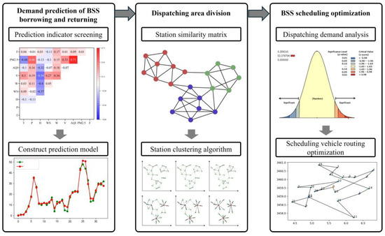
Figure 1.
Public bicycle dispatch framework based on the spatiotemporal characteristics of borrowing and returning demands.
3.1. Prediction Method for Public Bicycle-Borrowing and -Returning Demands
3.1.1. Prediction Indicator Screening
To avoid multicollinearity among characteristic variables of public bicycle-borrowing and -returning demands, the Pearson correlation coefficient is used to measure the correlation among bicycle use frequency, meteorological indicators, and air quality indicators (see Equation (1)).
The correlation coefficient, , represents the correlation between variable X and variable Y. When , there is a positive correlation between the variables. When , there is a negative correlation between the variables. The larger the absolute value of , the higher the degree of correlation between the variables. and are the observed values of variables X and Y, respectively; and are the sample means of variables X and Y.
Based on the results of the correlation coefficient calculation between variables, variables with a low correlation to bicycle usage frequency and those with multicollinearity are screened out.
3.1.2. Random Forest Regression Prediction Method
The random forest method can address both classification and regression problems, which primarily depend on whether each tree in the random forest is a classification tree or a regression tree. For regression trees, the principle employed is minimizing the mean squared error. Specifically, for any split feature T, given datasets and generated by any split point p, the final feature and feature value split point are determined to minimize the mean squared error of the collections in , and , while also minimizing the sum of the mean squared errors of and (see Equation (2)).
where is the sample output mean of dataset and is the sample output mean of dataset . The regression prediction of a random forest is the mean of the predictions of all trees.
3.2. Dispatch Area Division Method
The division of public bicycle dispatch areas aims to balance each area so that dispatch vehicles can complete their tasks in the shortest time possible, meeting the demands for bike borrowing and returning within peak periods. To minimize the travel costs of dispatch vehicles, it is advisable to include stations that are close in distance and relatively concentrated within the same area. However, both public bicycles and dispatch vehicles operate within the actual road network. Therefore, when dividing the areas, the measurement of the spatial distance between rental points should use the road network distance between the rental points, which is more realistic than straight-line distance.
On the other hand, public bicycles exhibit significant self-flow characteristics. The borrowing and returning behaviors of users cause bikes to flow between stations, and this flow is generally bidirectional, resulting in certain correlations between rental points. To adhere to the rules of PBS operation, it is advisable to ensure balance between borrowing and returning bikes within the same area, avoiding cross-area dispatching and including rental points with strong correlations in the same dispatch area.
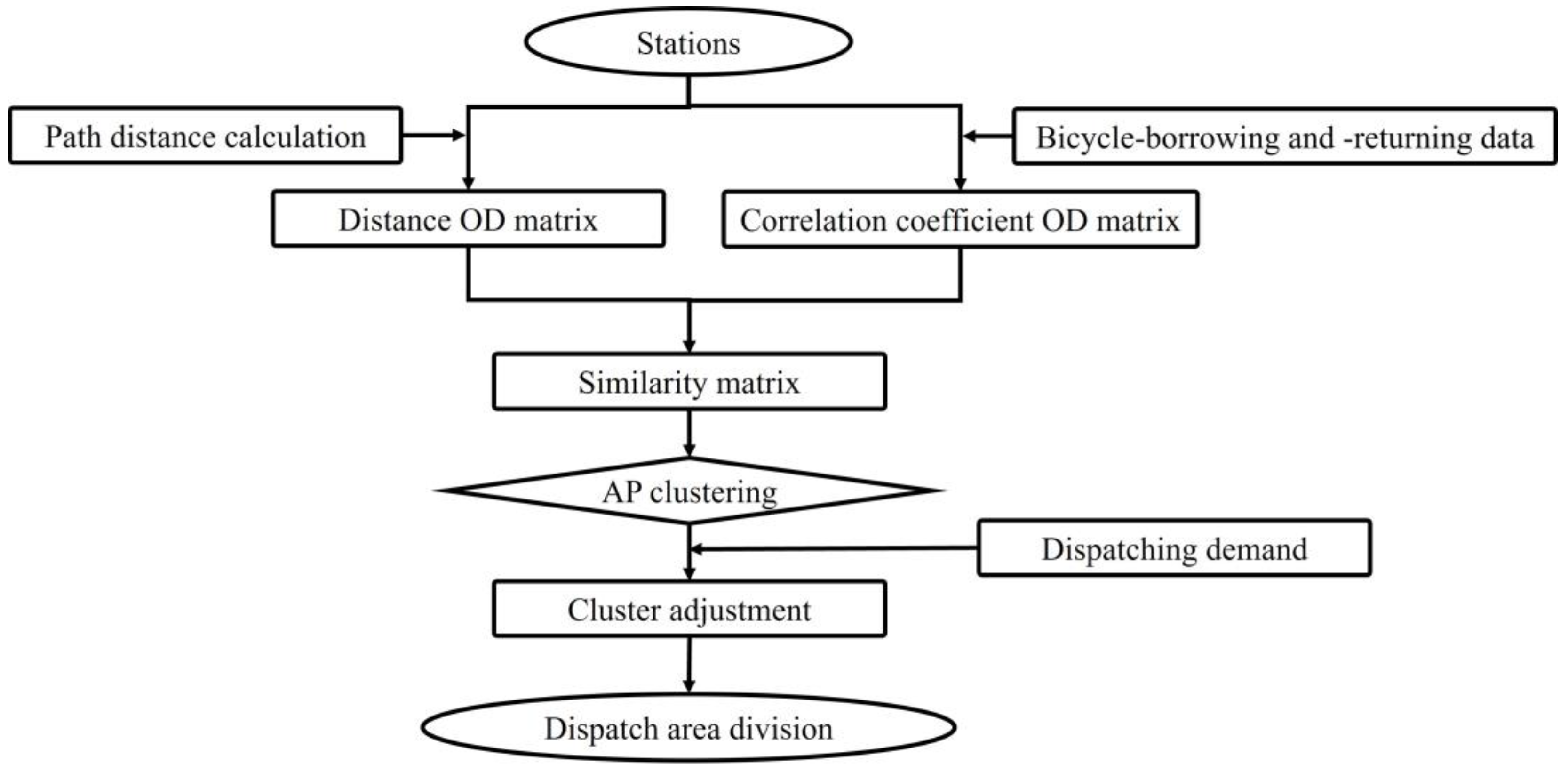
In summary, factors considered when dividing dispatch areas in this paper include road network distance between rental points, correlation strength, and balance of borrowing and returning demands within the area. This paper simultaneously considers the goals of road network distance between rental points, correlation strength, and balance of borrowing and returning demands within the area. By defining a distance measurement parameter that integrates rental point coordinates and correlation strength attributes, a dispatch area division model is constructed; then, the affinity propagation (AP) spatial clustering algorithm is used to solve it. Subsequently, adjustments are made based on the directional borrowing and returning demands at rental points in each divided area, land use types, and other characteristic attributes to ensure balance in dispatch demand within the area and obtain the final dispatch area division scheme. Figure 2 illustrates the process of dispatch area division.

Figure 2.
Flow chart of dispatch area division.
3.2.1. Definition of Parameters
The division of dispatch areas is aimed at enhancing vehicle dispatch efficiency. While considering the path distance between stations, it is essential to fully leverage the self-balancing characteristics of public bicycle flow, ensuring minimal imbalances in borrowing and returning within the same dispatch area, thus avoiding long-distance cross-area dispatching. The identification of the shortest paths between rental points and the calculation of path distances must be based on real road network data. In this paper, the calculation of path distances between stations is performed by using the cycling route planning and distance calculation functionalities provided by Baidu Maps Open Platform.
Let us assume that there are n public bicycle rental points involved in the division of dispatch areas and that the number of divided dispatch areas is k. B represents the set of stations, and Q denotes the set of dispatch areas. D represents the matrix of shortest-path distances between stations, where represents the shortest-path distance from station i to j. C represents the matrix of OD correlation coefficients between stations, where represents the OD connectivity count from station i to j.
The interrelationship between stations essentially represents the correlation between the borrowing and returning of bicycles between two stations. In this paper, the interstation OD connectivity count is defined to reflect the frequency of bicycle flow between stations. A higher connectivity count, denoted by , indicates a stronger borrowing and returning relationship between the stations. The calculation of the interstation connectivity count () between stations i and j within unit time t is shown in Equation (5).
where and represent the returning and borrowing correlation coefficients, respectively, from station i to j. Subsequently, aiming to minimize the imbalance between borrowing and returning within the designated dispatch areas, the imbalance rate (R) of borrowing and returning in the public bicycle system is established (see Equation (6)).
where and denote the quantity of bicycles borrowed and returned, respectively, within dispatch area j. For set of dispatch areas Q, the total borrowing and returning volume across all areas is represented as , and the sum of borrowing and returning imbalances is . The imbalance rate (R) reflects the overall borrowing and returning imbalances among the k areas. A higher R indicates larger imbalances between borrowing and returning within each dispatch area, suggesting higher demand for inter-area dispatch. Conversely, a lower R indicates smaller imbalances within each dispatch area, implying a relatively balanced state of borrowing and returning within the areas, thus indicating a more reasonable division of dispatch areas.
3.2.2. Station Similarity Matrix
Next, an approach is proposed in this paper to combine the spatial relationship between stations with the correlation between the borrowing and returning of bicycles. It is achieved by integrating the actual distance between stations with their associated attributes to establish the station similarity () (see Equations (7) and (8)).
where denotes the correlation coefficients between stations i and j, and represent the maximum and minimum values of correlation coefficient matrix between stations, and represents the intensity coefficient of borrowing and returning vehicles between stations i and j.
In essence, expresses the spatial distance between rental stations, where a larger value indicates a greater distance between stations, fewer borrowing and returning transactions, and lower similarity between rental stations. This contradicts mathematical logic. To ensure consistency between numerical values and mathematical logic, the association matrix is constructed by taking the negative of the similarity (see Equation (9)).
3.2.3. AP Clustering Algorithm
The dispatch area division based on the association matrix in this paper results in a concentrated distribution of stations within each class, while also ensuring strong borrowing and returning relationships between stations within the region. Furthermore, efforts are made to balance the borrowing and returning demands within the dispatch region to reduce the frequency of inter-regional dispatching and decrease the workload of dispatching.
Cluster adjustment primarily involves exchanging stations between different regional classes to achieve a balance in the borrowing and returning demands within each dispatch region. Initially, the total difference in borrowing and returning demands for each class is calculated separately. Based on the positive or negative sign of the differences, adjustments are made between complementary regional classes, ensuring that the exchanged stations do not overly increase the dispersion within the new class and that the spatial distance between rental points within each dispatch region remains within acceptable ranges. The AP clustering algorithm is adopted for dispatch area division, with the algorithm’s main process being outlined as follows:
Step 1: Construct the similarity matrix (S) among data points.
Step 2: Initialize the algorithm with the given parameter values.
Step 3: Compute and update the attractiveness matrix.
Step 4: Compute and update the attribution matrix.
Step 5: Update the attractiveness and attribution matrices based on the convergence coefficient (γ).
Determine whether a data point is a cluster center based on the value of a + r. Repeat steps 2, 3, and 4 until matrix stability is achieved or the maximum number of iterations is reached, terminating the algorithm.
3.3. Dispatch Demand Analysis
Conducting public bicycle dispatching requires clear delineation of three crucial parameters: station status, time windows, and dispatch demand. This involves determining whether a station needs bicycles to be dispatched in or out based on its status and borrowing–returning trends, as well as establishing the time windows and quantities for bicycle redistribution at each station.
3.3.1. Station Status Determination
Station status can be described by the ratio of available bicycles to station capacity, reflecting the status of empty or full docks at each station. Station status can be categorized into three situations, full, empty, and normal, detailed as follows:
- Full: This occurs when the number of available bicycles at a station equals its capacity. In this state, the station can provide bicycle-borrowing services but cannot accept returned bicycles from users. If users need to return bicycles, they either rely on others to borrow bikes or seek nearby stations with available docks, which can inconvenience users significantly. When formulating dispatch optimization plans, it is essential to avoid stations reaching full capacity and to conduct advance dispatching to ensure available docks for bicycle returns.
- Empty: This happens when the number of available dock spaces equals zero at a station. In this scenario, the station can accept returned bicycles but cannot provide bicycles for borrowing. If users need to borrow bicycles, they must wait for others to return bicycles or find nearby stations with available bicycles to borrow. Similarly, dispatch optimization plans should avoid situations where stations run out of dock spaces, and bicycle replenishment should occur before stations become completely empty.
- Normal: This state indicates that the number of bicycles and available dock spaces at a station can facilitate regular bicycle-borrowing and -returning activities by users. The goal of bicycle dispatching is to transition stations from a near-empty or -full state back to a normal state.
3.3.2. Time-Window Determination
During peak hours, public bicycle systems experience heightened mobility, leading to stations frequently entering abnormal states of ‘no bikes available for borrowing, no docks available for returning’. Hence, the proactive balancing of bicycles is necessary. The dispatch time window refers to the timeframe during which stations are available for redistribution services, and it can be divided into an expected time window and an acceptable time window. If the dispatch service provided by dispatching vehicles exceeds the expected time window, it will decrease the efficiency of the public bicycle system.
Let us assume that the initial dispatch time is , the initial number of bicycles at station i is , and the capacity of the station is . The time when dispatching vehicles arrive at station i is , and the imbalance of bicycle borrowing and returning at station i per unit time is denoted by .
When exceeds 0, indicating station i requires bicycles to be transferred in, should satisfy
When falls below 0, indicating station i requires bicycles to be transferred out, should satisfy
When station i is in a normal state, the ratio of the number of bicycles to the station’s capacity () should remain within a reasonable range, . As approaches the upper or lowerlimit of the station’s dispatch time window, the expected dispatch time window can be calculated based on the predicted borrowing and returning demands of the station.
3.3.3. Dispatch Demand Analysis
The dispatching demand denotes the number of public bicycles that the station needs to transfer in or out in a certain period of time. It can be analyzed according to the current situation and the historical law of borrowing and returning vehicles of the station. When bicycle mobility is high, accurately calculating the optimal redeployment demand becomes challenging. In practical applications, it is essential to maintain the ratio of bicycle docks to available bicycles at stations within the range of [] after redeployment. The redeployment demand for station i should satisfy Equation (16), and Equation (16) can be further expressed as Equation (17).
The range of values for station redistribution can be determined by using Equation (17). When determining the specific amount of redistribution, stations with inbound redistribution demands are prioritized, followed by determining the outbound redistribution amount for stations based on proximity. The goal is to ensure that the total inbound redistribution quantity equals the total outbound redistribution quantity within the dispatch area.
3.4. Regional Dispatch Vehicle Route Optimization Model
Public bicycle dispatching should reduce dispatching costs while ensuring efficiency, and whether bike-borrowing and -returning operations can be conducted within the target time period is of concern to users. Therefore, when determining dispatch optimization objectives, this paper simultaneously considers the optimization of dispatch vehicle activation, operational costs, and time penalty costs, with a focus on time costs. In summary, the optimization problem of peak-period vehicle dispatch can be described as follows: Given the predicted dispatch demands of each station, dispatch vehicles depart from the dispatch center, travel to stations with dispatch demands to redistribute bicycles, and finally return to the dispatch center. The goal is to determine the number of dispatch vehicles and their routes to minimize total dispatching costs. Based on historical operation data of public bicycles, this paper makes the following assumptions before establishing the mathematical model for optimizing dispatch vehicle routes:
- We assume that the location of the regional dispatch center, the capacity of dispatch vehicles, and the maximum travel distance are all known parameters.
- To simplify the solution process, we assume that the maximum carrying capacity of dispatch vehicles exceeds the dispatch demand of each station.
- We assume that dispatch vehicles depart from the regional dispatch center, complete their dispatch tasks, and finally return to the center.
- Each station is served once in a single dispatch operation and is only served once.
- We assume good road traffic conditions during dispatching and do not consider special situations such as traffic congestion.
3.4.1. Definition of Parameters
- Vehicle Activation and Operating Costs
The vehicle activation cost is determined by multiplying the required number of dispatch vehicles by the fixed activation cost per vehicle. The dispatch vehicle operating cost equals the product of the vehicle’s travel distance and the unit travel cost per distance, as expressed in Equation (18).
where denotes the activation cost of a dispatch vehicle, K and k are the amount and number of dispatch vehicles, and represents the cost of dispatch vehicle in unit distance.
- 2.
- Penalty Function
In the optimization of dispatch vehicle routes during peak commuting hours, where users are particularly sensitive to time constraints, failure to meet users’ demands implies a decrease in the system’s service level. Therefore, it is necessary to constrain the arrival time of dispatch vehicles within an acceptable range for users. This study introduces a penalty cost for deviation from the required arrival time. The penalty increases proportionally with the deviation from the time window, reflecting the degree of departure from user expectations. The penalty cost for deviation from the arrival time window also reflects user satisfaction with the use of public bicycles. The following assumptions are made regarding the penalty function:
- When a dispatch vehicle arrives at the station within the required time window, the penalty is zero.
- If a dispatch vehicle arrives at the station within the acceptable time window, the penalty is linearly related to the deviation from the expected time window.
- If a dispatch vehicle arrives after the station’s acceptable time window, a significant penalty is applied to emphasize the importance of timely arrivals during peak hours.
Based on these assumptions, a penalty function for deviation from the expected arrival time is established.
The time penalty cost incurred by dispatch vehicles serving station i is represented by , where denotes the arrival time of the dispatch vehicle at station i. M represents the penalty cost incurred when the arrival time of the dispatch vehicle falls outside the acceptable time window, set to a sufficiently large positive value to prevent the algorithm from sacrificing service at stations within the time window to reduce dispatch vehicle operating costs. and denote the lower and upper bounds, respectively, of the expected demand scheduling time window for the station. and represent the lower and upper bounds, respectively, of the acceptable demand scheduling time window for the station. and represent the penalty cost coefficients when the dispatch vehicle arrives early or late.
3.4.2. Model Construction
- Objective Function
Considering the aforementioned analysis, the objective function of the dispatch optimization model is formulated as shown in Equation (21).
where indicates the sum of activation cost, operation cost and penalty cost of dispatch vehicles. The penalty cost represents the cost incurred when dispatch vehicles fail to arrive within the expected time window.
- 2.
- Constraints
The definitions of relevant parameters in the vehicle dispatch model based on regional division include the following: The maximum carrying capacity of dispatch vehicles, denoted by Q. There are n stations within the corresponding dispatch region. The dispatch demand at station i is represented by . When , station i has a dispatch demand for outgoing bicycles; when , station i has a dispatch demand for incoming bicycles. The dispatch center for the region is denoted as 0. represents the service time of dispatch vehicles at station i, and represents the travel time of dispatch vehicles from station i to station j. The following apply:
- The number of vehicles participating in the dispatch is no more than K.
- At the beginning of dispatch, vehicles depart from the dispatch center and eventually return to it.
- During the dispatch process, the number of bicycles on the dispatch vehicles remains between 0 and the maximum capacity.
- represents the moment when the dispatch vehicle arrives at station j, with the previous station before arrival being i.
- Dispatch vehicles enter and exit the same station once during the dispatch process.
- Dispatch vehicles must leave after arriving at a station.
3.4.3. Solution Algorithm
Most traditional search and optimization algorithms, especially those based on gradient descent, tend to converge prematurely into local optima rather than finding the global optimal solution. In contrast, the GA can search for the optimal solution with greater ease and efficiency. Therefore, the genetic algorithm is utilized in this study to solve the regional dispatch vehicle route optimization model. The specific algorithm design is outlined below.
- Encoding and decoding method
Vehicle dispatch entails a sequence-based combinatorial optimization problem, and a natural number encoding method is employed. Let us assume that there are K dispatch vehicles at the dispatch center and n stations in the dispatch region, with 0 denoting the dispatch center. As the required number of dispatch vehicles is uncertain beforehand, 0 is not integrated as a path delimiter into the chromosome structure during encoding. Instead, stations with dispatch demands are sequentially added to a chromosome. This intuitive encoding method based on station permutation ensures that each station is serviced only once, simplifying the handling of model constraints and facilitating genetic operations. The decoding process follows a procedure similar to encoding, where values from the chromosome are sequentially inserted into a newly initialized path. When the insertion of a value leads to the total demand of the path exceeding the maximum carrying capacity of the dispatch vehicles, it is replaced by 0, initiating the construction of a new path until all stations are accommodated in the path.
- 2.
- Population initialization
The initial population serves as the starting point for genetic algorithm evolution. It is generated randomly to achieve a uniformly distributed initial population across the solution space. The size of the population often influences the algorithm’s execution efficiency and the final optimization outcomes. A population that is too small may result in the algorithm getting trapped in local optima with poor optimization performance, while an excessively large population would increase the temporal and spatial complexity of algorithm execution. When the chromosome length is not excessive, a population size ranging from 20 to 200 is deemed suitable.
- 3.
- Constraint handling and fitness evaluation
Considering the characteristics of the dispatch model constraints, constraints such as stations being serviced only once are manifested in the chromosome encoding. Additionally, time-window constraints and the constraint of the maximum carrying capacity of the dispatch vehicles need to be addressed. Time-window constraints are incorporated into the objective function in the form of time penalty costs, while the constraint of maximum carrying capacity is handled by using a penalty function defined as follows:
The fitness evaluation of individuals in the population is a crucial basis for genetic operations. The fitness function value is a non-negative number, with larger values indicating a higher probability of individuals producing offspring. As the optimization objective of this study is to minimize the function value, the fitness function is represented as Equation (32).
where i represents the i-th chromosome in the population; denotes the penalty cost coefficient for the maximum carrying capacity; represents the penalty function value for the maximum carrying capacity; denotes the load from station i to station j for dispatch vehicle k; indicates the objective function value corresponding to chromosome i, representing the dispatch cost in this paper; and denotes the fitness value of chromosome i.
- 4.
- Genetic Operations
Genetic operations encompass selection, crossover, and mutation. This paper adopts the roulette wheel selection method based on stochastic sampling as the selection operator. The crossover operator employs the partially matched crossover method suitable for integer encoding problems, along with an inversion mutation operator to prevent the premature convergence of the algorithm.
- 5.
- Termination Condition
This study controls the algorithm’s execution time and solution accuracy by predefining the number of evolution generations. When the number of evolution generations reaches the preset value, the iteration ceases, and the optimal chromosome corresponding to the dispatch path is output.
4. Results
4.1. Prediction of Public Bicycle Demand
4.1.1. Feature Variable Selection
- Meteorological and Air Quality Indicators
The original meteorological and air quality data contain numerous data indicators, some of which are evidently unrelated to the research objective. In this preliminary stage, the data indicators shown in Table 2 are selected.
Table 2.
Indicator description of meteorological and air quality.
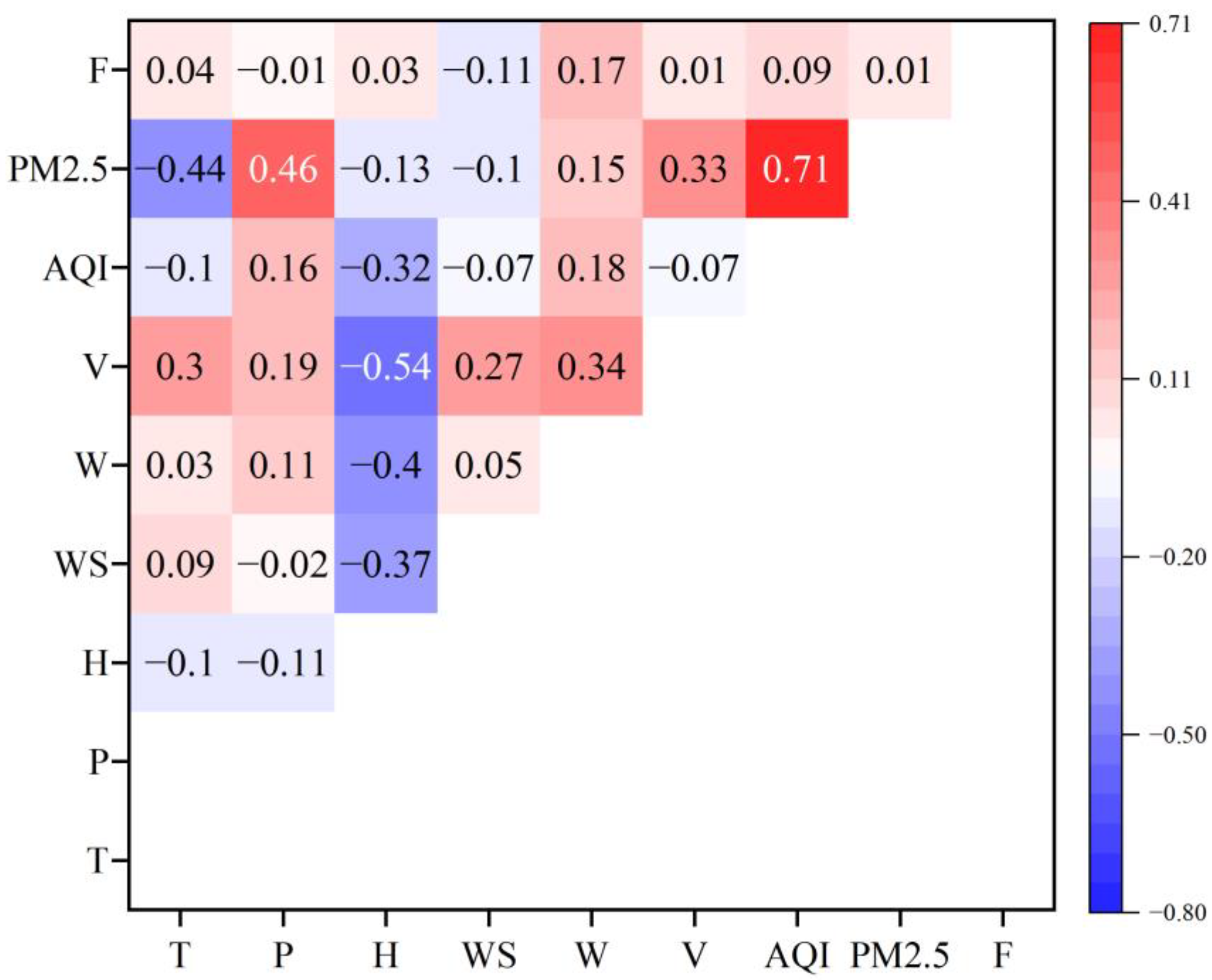
This paper utilizes the Pearson correlation coefficient to screen an appropriate set of parameters for public bicycle demand forecasting models, thereby constructing an accurate prediction model. Initially, parameters with higher correlation to public bicycle demand are prioritized for selection. Furthermore, parameters exhibiting multicollinearity are eliminated to the greatest extent possible. The correlation coefficients between various meteorological indicators and the frequency of bicycle usage (F) are calculated, as shown in Figure 3. It can be observed that there is a strong correlation between AQI and PM2.5, as well as between air pressure (P) and temperature (T). Similarly, there is a significant correlation between relative humidity (H) and horizontal visibility (V) and between weather (W) and relative humidity (H). Considering the overall correlation between each meteorological factor and the frequency of usage (F), it is decided to eliminate the three indicators PM2.5, air pressure (P), and horizontal visibility (V).

Figure 3.
Correlation coefficient matrix.
- 2.
- Temporal Features
The demand for public bicycles varies at different times of the day and on weekdays versus weekends (including holidays) and also shows seasonal differences across different months. Therefore, different times of the day, days of the week, whether it is a weekday, and the month are important feature variables for predicting bicycle demand.
Different times of the day refer to intervals from 5:00 to 22:00, with a data collection interval of 30 min, resulting in a total of 34 time intervals. For example, 1 represents 5:00–5:30, and 34 represents 9:30–10:00, and so on. The selection of the time ranges from 5:00 to 22:00 is because the demand for public bicycles during other times is extremely low, almost negligible, and thus not considered in this study. Regarding the selection of the prediction time intervals, if the intervals are too small, there may be significant fluctuations in bicycle demand, leading to many samples with zero data and increased random interference during prediction. Conversely, if the intervals are too large, it may not accurately represent the changing trend of demand, resulting in delays in subsequent scheduling. Hence, based on the actual changes in demand for public bicycles studied in this paper, a time interval of 30 min is determined.
- 3.
- Station Locations
Public bicycle station locations vary, and so do the borrowing and returning demands, exhibiting spatial distribution patterns. Additionally, stations in different land use types demonstrate borrowing and returning volumes that align with the characteristics of different land use types. Therefore, station locations and land use types are chosen as feature variables for the predictive model.
In summary, the selected predictive factors in this study include meteorological factors, temporal features, and station location features, as detailed in Table 3.
Table 3.
Summary of predicted parameters.
Based on the selected influencing variables described above, feature vectors for each time window at each station were constructed in this study. Station actual borrowing and returning volumes were taken as target values, and random forest prediction models were separately trained for station borrowing demand and returning demand. The public bicycle-borrowing and -returning volume data from July 2016 to June 2017 in Ningbo City were divided into training, validation, and test sets in an 8:1:1 ratio. The training set was used for model learning and training, the validation set for model parameter adjustment, and the test set for model performance evaluation.
4.1.2. Model Parameter Settings
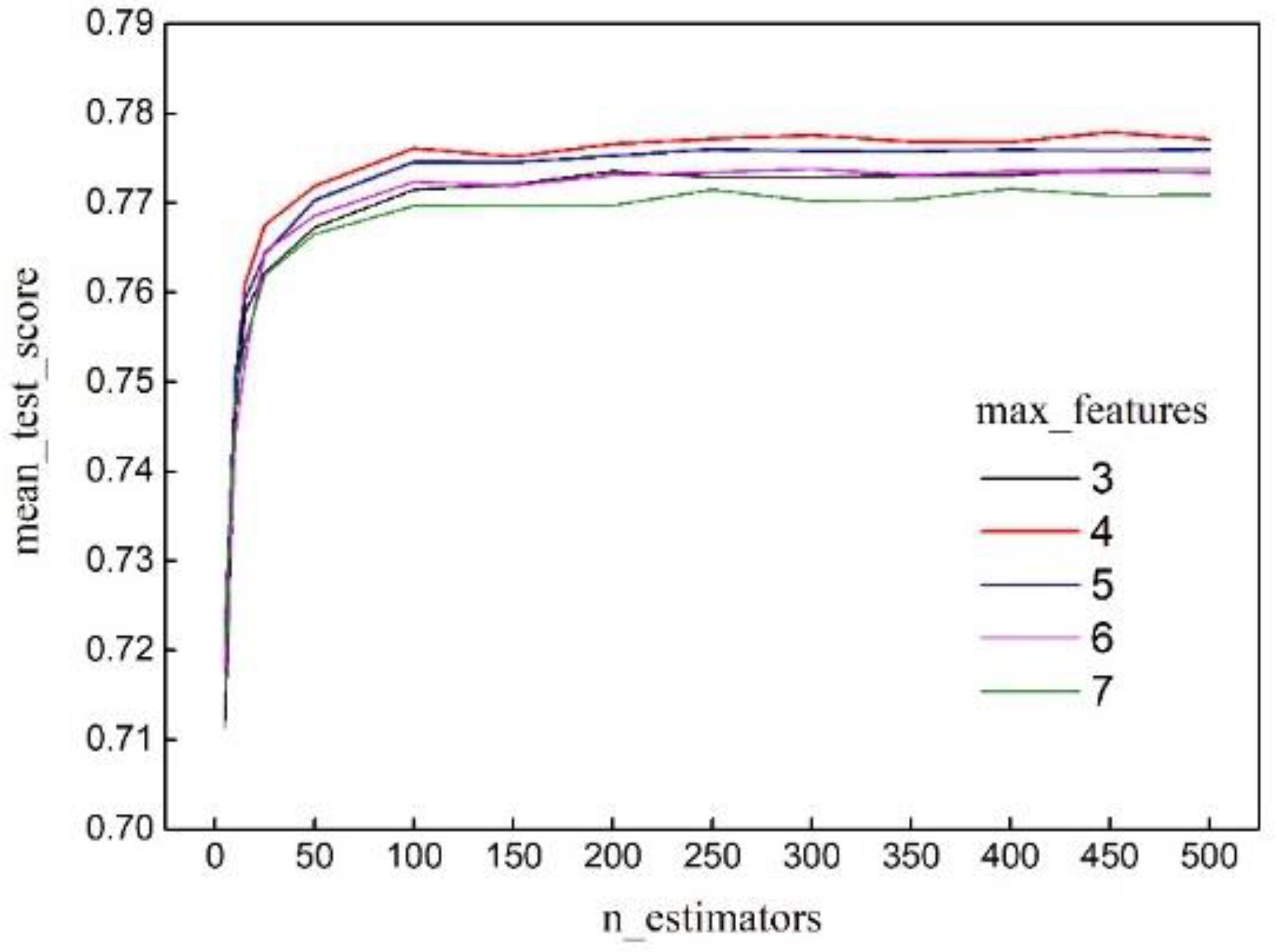
The demand prediction model proposed in this paper is constructed based on the predictive parameters outlined in Table 3. In Python, the GridSearchCV function was invoked, with the model evaluation metric parameter ‘scoring’ being set to ‘r2′ and the number of cross-validation folds being set to 5. Specifically, ‘mean_test_score’ represents the average score of the validation set, serving as a measure of the predictive accuracy of the prediction model. Figure 4 illustrates the model accuracy under different parameter combinations of the random forest prediction model. The horizontal axis represents the variable of the number of decision trees, while the vertical axis displays the model scores obtained when experimenting with maximum feature numbers ranging from 3 to 7. The parameter ‘n_estimators’ defines the number of trees, or estimators, in a random forest model. When the value of ‘n_estimators’ is set too high, the model may overfit, meaning it becomes too complex to generalize well to unseen data. Therefore, it is essential to select a smaller ‘n_estimators’ as a model parameter while still achieving a satisfactory level of predictive accuracy. It can be observed that when ‘n_estimators’ exceeds 100, the increment in model accuracy tends to plateau. Increasing ‘max_features’ generally improves the classification ability of each tree since there are more features to choose from at each node. However, it also increases the correlation between any two trees in the forest, leading to an increase in classification error rates. Additionally, increasing ‘max_features’ can slow down the algorithm. Therefore, a balanced value of ‘max_features’ should be selected. The highest model accuracy is achieved when ‘max_features’ is set to 4, with the corresponding model scores peaking at 300 and 450 decision trees, respectively. Considering both computational efficiency and model accuracy, the parameter combination of ‘max_features’ as 4 and 300 decision trees was selected to build the model.

Figure 4.
mean_test_score changes as n_estimators and max_features increases.
4.1.3. Prediction Results
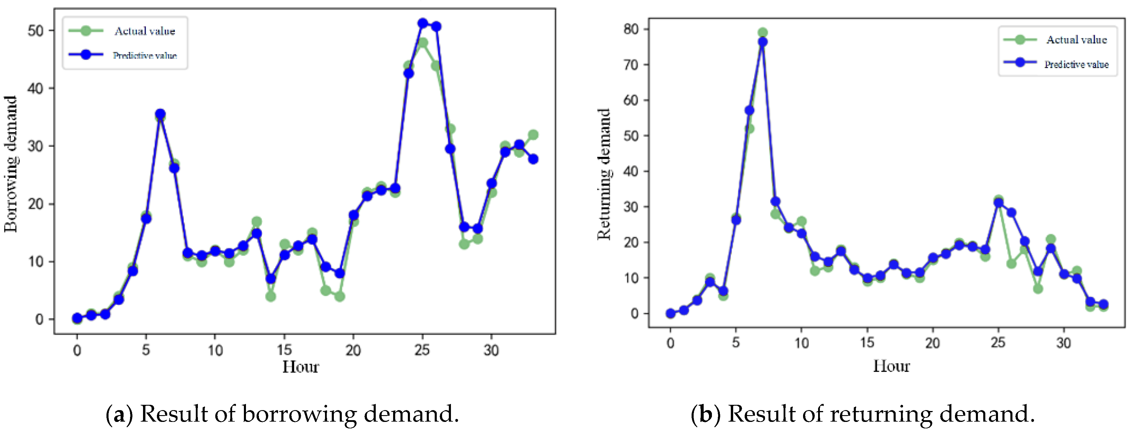
Taking the East Gate station in Ningbo City, which has the highest demand for bicycle borrowing and returning, as an example, comparison graphs of the predicted and actual demand for borrowing and returning bicycles at this station were plotted (see Figure 5). The results indicate that for specific stations, the predicted demand closely approximates the actual demand, meeting the accuracy requirements for vehicle dispatching. Figure 5 indicates the overall trends in bicycle-borrowing and -returning demands, both peaking during morning and evening peak hours. Specifically, Figure 5a represents the pattern of borrowing demand, indicating that the demand during the evening peak is significantly higher than that during the morning peak. Concurrently, Figure 5b illustrates the pattern of returning demand, showing that the returning demand during the evening peak is noticeably lower than that during the morning peak. This disparity in patterns determines the role of this public bicycle station within the PBS system.
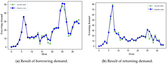
Figure 5.
Bike-sharing demand prediction of renting and returning bikes.
To validate the effectiveness of the proposed prediction method in this paper, random forest prediction models for both bicycle-borrowing demand and bicycle-returning demand were constructed separately. The performance of the models was tested by using the partitioned test dataset, and the results are presented in Table 4. In general, when the goodness-of-fit R2 of a prediction model is greater than 0 and less than 1, a higher R2 value indicates higher accuracy of the regression fit. When R2 exceeds 0.8, the linear relationship of the prediction model is significant, indicating a high degree of fit for the predicted results. The coefficients of determination (R2) are all above 0.8, indicating high prediction accuracy. Moreover, both the mean absolute error and root mean square error of borrowing and returning volumes fall within the allowable error range, indicating the reliability of the random forest prediction models constructed in this paper.
Table 4.
Effect of prediction models of renting bikes and returning bikes.
4.2. Management Area Division
4.2.1. Similarity Matrix Construction
In practice, the round-trip paths between two stations may not be the same, i.e., the distances from station i to j and from station j to i should be calculated separately. However, due to the large number of stations involved in this study, calculating round-trip distances between all pairs of stations would significantly increase the number of requests to the Baidu Maps 2024 server. Frequent data retrieval may face restrictions. Therefore, this paper only computed the one-way path distances between stations. In this paper, the actual distances between public bicycle stations were obtained through the Baidu Map API. Within the Baidu Map API, the high-performance batch path calculation function, along with real-time traffic conditions, was leveraged to batch-calculate the route distances and travel times for multiple origin–destination pairs. The specific steps are as follows: A Python program was developed to read all station coordinates and generate OD coordinate lists by using a loop code. These OD coordinate lists were then used as input to access the Baidu Maps API, obtaining the actual path distances between stations. Subsequently, the distance data obtained were written into a distance matrix by using loop control, resulting in a symmetric matrix of size 1093 × 1093. A summary of the matrix is presented in Table 5.
Table 5.
Actual path distance matrix of Ningbo public bicycle stations (meters).
The calculation method of the inter-station similarity matrix involves accessing the database by using Python, where a loop control program is developed to sequentially tally the total borrowings and returns for each station, as well as the borrowings and returns for OD station pairs, thereby obtaining the borrowing matrix and returning matrix for OD stations. Following the method described in Section 3.2 of this paper, matrix operations were performed by using the Python extension library NumPy to compute the inter-station connectivity matrix, as shown in Table 6.
Table 6.
Similarity matrix of Ningbo public bicycle stations (meters).
4.2.2. Management Area Division
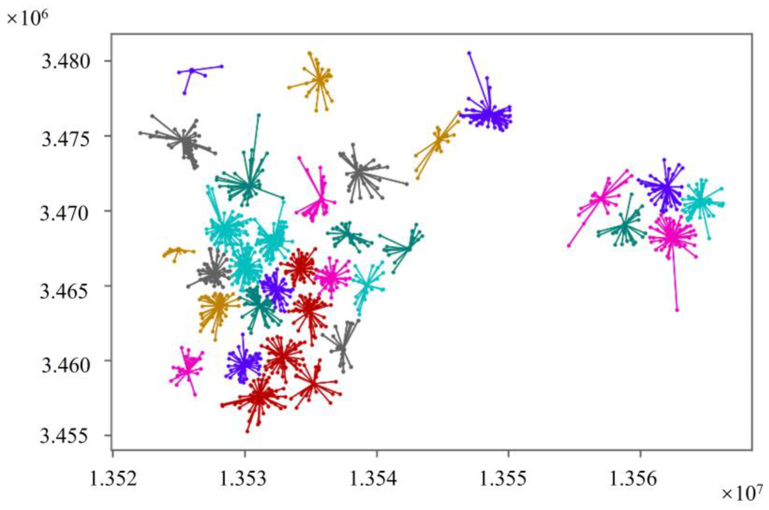
The scheduling region partitioning model was solved by invoking the Affinity Propagation algorithm from the Python library. In the AP algorithm solving process, the computed similarity matrix was used as input, with the reference preference set to the median of the similarities. The affinity parameter was set to precomputed, and the damping factor was set to 0.7. The scheduling region partitioning model was then solved, resulting in the partitioning of 1093 stations into 33 sub-scheduling regions. The partitioning results are illustrated in Figure 6, where each color-coded cluster represents a scheduling region, and each radiating center denotes a cluster centroid.
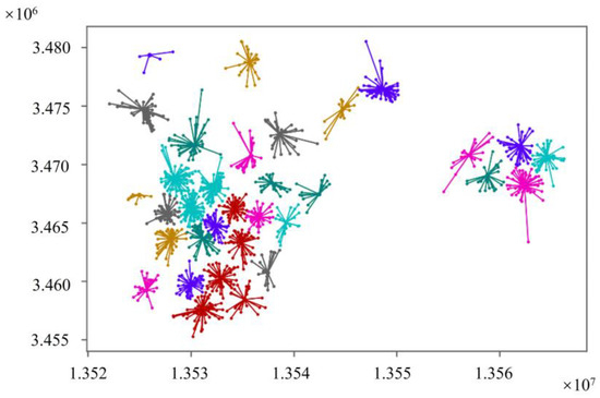
Figure 6.
Result of management areas division.
Cluster adjustment was completed according to the method described in Section 3.2 of this paper. To demonstrate the effectiveness of the scheduling region partitioning results based on actual path distances, a scheduling region partitioning model based on Euclidean distance was also established. Based on the two partitioning results, the imbalance rate indicator (R) of borrowing and returning bikes in the scheduling regions was calculated (see Table 7). A smaller R value indicates a closer balance between borrowing and returning bikes within the region and a lower rate of inter-regional travel, which is conducive to scheduling balance. It can be observed that the scheduling regions partitioned based on actual path distances exhibit a significantly greater reduction in the imbalance rate compared with those based on Euclidean distance. It suggests that the scheduling region partitioning model proposed in this paper is effective. The management area division method that considers actual path distances is superior to the method that considers Euclidean distances, indicating that the actual travel costs for OD pairs do not fully align with the Euclidean distances between stations. This also demonstrates the significance of considering the actual distance attributes between stations for the optimization of PBS rebalancing.
Table 7.
R value based on actual path distance and Euclidean distance.
4.3. PBS Rebalancing Scheme
4.3.1. Station Allocation Demand
- Overview of Scheduling Regions
Based on the partitioning results of the public bicycle scheduling regions, the 26th scheduling region in Haishu District of Ningbo City was selected as the research scope. This region encompasses 22 stations, numbered sequentially, with the dispatch center numbered as 0, as shown in Table 8.
Table 8.
Location of stations.
- 2.
- Bicycle Dispatch Quantity at Stations
During the weekday morning peak hours, stations in the 26th scheduling region were subjected to dispatching. The morning peak period was determined based on the historical borrowing and returning data of each station in the area, with the peak hours set from 7:00 to 8:30. For research purposes, we focused on the hour from 7:00 to 8:00. Following the methodology outlined in Section 3.3, the borrowing and returning demands during the corresponding research period were predicted. It was assumed that the initial state of the stations was known (in practical applications, real-time station monitoring can be employed). Station status thresholds were set to [0.2, 0.8], thereby determining the status of each station, dispatch time window, and deployment volume range. The specific determination of deployment volume prioritized satisfying stations with incoming demand. Then, based on the total incoming demand, the deployment volume for stations with outgoing demand was determined. The resulting morning peak station dispatch demands are shown in Table 9. The acceptable time-window values in the table are hypothetical and can be obtained through actual surveys based on station land use types during application.
Table 9.
Bicycle dispatch demand at stations.
4.3.2. Algorithm Parameter Setting
The parameter settings for the scheduling optimization model solving algorithm are shown in Table 10.
Table 10.
Algorithm parameter setting.
4.3.3. Results
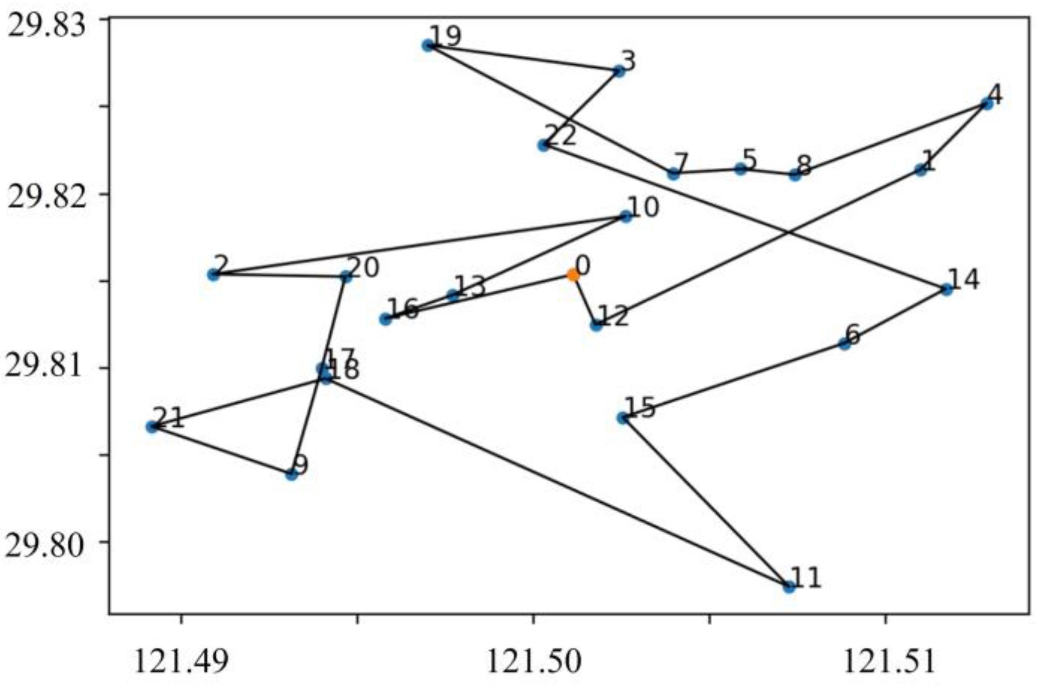
Then, the optimal rebalancing scheme based on the GA algorithm is shown Figure 7. The optimal rebalancing order is 0-12-1-4-8-5-7-19-3-22-14-6-15-11-18-21-9-17-20-2-10-13-16-0. The value of the purpose function is 1012.25. The working time of the dispatch vehicle is 1.36 h. Moreover, this study also solves the bike-sharing rebalancing problem with the Taboo search algorithm (TSA). The results of GA and TSA are shown in Table 11.
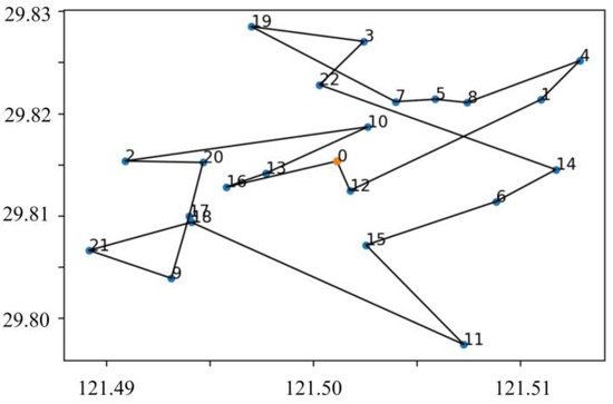
Figure 7.
Result of public bicycle dispatching scheme.
Table 11.
Results of GA and TSA.
Based on the solution results, it can be observed that based on the scheduling region division proposed in this paper, when conducting scheduling optimization design, both algorithms indicate that only one dispatch vehicle needs to depart from the dispatch center and sequentially connect stations with dispatch demands along the designed route to complete the balancing deployment task. By comparing the results of the two algorithms, it can be seen that the optimal solution obtained by the genetic algorithm proposed in this paper corresponds to a lower objective function value, and the duration required for the dispatch vehicle to complete the same deployment task is shorter.
5. Conclusions
This paper presents a public bicycle dispatch framework based on the spatiotemporal characteristics of borrowing and returning demands. Firstly, the spatiotemporal distribution characteristics of public bicycle-borrowing and -returning demands are explored, and the OD connectivity numbers are defined to analyze the strength of inter-area connections between stations. Secondly, based on the time-varying demand characteristics of stations, a random forest prediction model is constructed, with meteorological factors, time features, and station locations as feature variables, and station borrowing and returning demands as target variables. Finally, bicycle dispatch areas are divided based on the actual path distances between stations and OD connectivity numbers, and a public bicycle dispatch optimization method for partitioning areas is established. Taking the PBS in Ningbo City as an example, the proposed dispatch balance optimization framework is validated. The main achievements of the paper are summarized below.
- Results on station borrowing and returning demand prediction
Addressing the issue of predicting public bicycle-borrowing and -returning demands, a random forest prediction method considering station land use types is proposed. A random forest prediction model is constructed with meteorological and air quality factors, time features, and station locations as feature variables, and station borrowing and returning demands at half-hour granularity as target variables. The model is validated by using actual operational data of public bicycles in Ningbo City, and the results show that the constructed model has high prediction accuracy and can be used as a basis for station dispatch.
- 2.
- Results on dispatch area division
Dispatch area division is essentially a spatial clustering problem. Addressing the shortcomings of existing research, this paper proposes a dispatch area division method that integrates actual path distances between stations and OD connectivity numbers. Taking the PBS in Ningbo City as an example, a similarity matrix that integrates station geographical locations and connectivity strengths is constructed, and the AP algorithm is used to divide the stations into 33 sub-dispatch areas. Compared with the results of management area division based on Euclidean distance, the imbalance rate of borrowing and returning in management area division based on the actual distance of the road network is reduced by 44.8%. The comparison shows that the proposed dispatch area division method can effectively improve the imbalance rate of borrowing and returning in dispatch areas.
- 3.
- Results on optimization of dispatch vehicle routes during peak periods
By analyzing the dispatch demand characteristics of PBS stations during peak periods, a dispatch vehicle route optimization model is constructed with dispatch vehicle cost and time penalty cost as objectives. A genetic algorithm is designed to solve the model based on objective values and constraints. Taking 22 stations in a certain dispatch area in Ningbo City as an example, the dispatch model is verified based on the genetic algorithm. The results show that only one dispatch vehicle is needed to complete the deployment task in a single dispatch area, and compared with the results obtained by the taboo search algorithm, the results obtained by the genetic algorithm designed in this paper are more optimal, achieving the optimization of public bicycle dispatch in the area. Additionally, compared with the TSA, the GA exhibits a 11.1% reduction in rebalancing time and a 40.4% reduction in trip cost. The TSA is an optimization technique based on local search which explores possible solutions in the search space to find the optimal solution. Moreover, the GA is an optimization technique based on the natural biological evolution process, simulating the processes of natural selection and genetic propagation to locate the optimal solution. The logical framework of the GA determines its faster solution speed and better optimization performance when addressing discrete problems such as public bicycle rebalancing.
This paper can provide technical support to urban transportation management departments and public bicycle operators, enhancing the effectiveness of public bicycle rebalancing strategies. For instance, operators and managers of PBSs can utilize the methodology proposed in this paper to select an appropriate number of trucks for rebalancing based on varying scheduling demands at different times, significantly reducing the operational costs of PBSs. Furthermore, the application of the research findings can contribute to promoting urban sustainability and mitigating traffic congestion. However, it must be acknowledged that this paper still has some limitations. The model proposed in this paper is relatively idealistic, overlooking practical scenarios such as traffic congestion. Future research will refine the model construction and align it with real-world scenarios to more precisely address practical engineering problems.
Author Contributions
Conceptualization, Z.L.; methodology, Z.L.; software, Z.L., Z.W. and C.G.; validation, Z.L., F.T. and H.C.; formal analysis, Z.L. and W.X.; investigation, Z.L.; resources, H.C.; data curation, F.T.; writing—original draft preparation, Z.L.; writing—review and editing, Z.L., F.T. and H.C.; visualization, Z.L.; supervision, H.C., Z.W. and C.G.; project administration, Z.L.; funding acquisition, Z.L. All authors have read and agreed to the published version of the manuscript.
Funding
This research was funded in part by the National Nature Science Foundation of China (grant No. 52302385), the Foundation of Hunan Province Educational Committee (grant No. 22C0173), the Changsha Major Science and Technology Special Project (kh2301004), the Open Fund of Hunan International Scientific and Technological Innovation Cooperation Base of Advanced Construction and Maintenance Technology of Highway (Changsha University of Science & Technology) (grant No. kfj220802), and the Hunan Provincial Natural Science Foundation of China (2023JJ30055, awarded to W.X.).
Institutional Review Board Statement
Not applicable.
Informed Consent Statement
Not applicable.
Data Availability Statement
The data used to support the findings of this study are available from the corresponding author upon request.
Conflicts of Interest
The authors declare no conflicts of interest.
References
- Liu, Z.; Chen, H.; Liu, E.; Hu, W. Exploring the resilience assessment framework of urban road network for sustainable cities. Phys. A Stat. Mech. Its Appl. 2022, 586, 126465. [Google Scholar] [CrossRef]
- Liu, Z.; Chen, H.; Liu, E.; Zhang, Q. Evaluating the dynamic resilience of the multi-mode public transit network for sustainable transport. J. Clean. Prod. 2022, 348, 131350. [Google Scholar] [CrossRef]
- Sun, D.D.; Ding, X. Spatiotemporal evolution of ridesourcing markets under the new restriction policy: A case study in Shanghai. Transp. Res. Part A Policy Pract. 2019, 130, 227–239. [Google Scholar] [CrossRef]
- Liu, Z.; Sun, D.; Chen, H.; Hao, W.; Wang, Z.; Tang, F. Resilience-based post-disaster repair strategy for integrated public transit networks. Transp. B Transp. Dyn. 2024, 12, 1–25. [Google Scholar] [CrossRef]
- Elhenawy, M.; Rakha, H.A.; Bichiou, Y.; Masoud, M.; Glaser, S.; Pinnow, J.; Stohy, A. A Feasible Solution for Rebalancing Large-Scale Bike Sharing Systems. Sustainability 2021, 13, 13433. [Google Scholar] [CrossRef]
- Pan, B.; Tian, L.; Pei, Y. The Novel Application of Deep Reinforcement to Solve the Rebalancing Problem of Bicycle Sharing Systems with Spatiotemporal Features. Appl. Sci. 2023, 13, 9872. [Google Scholar] [CrossRef]
- Nian, G.; Pan, H.; Huang, J.; Sun, D.J. Labor supply decisions of taxi drivers in megacities during COVID-19 pandemic period. Travel Behav. Soc. 2024, 35, 100745. [Google Scholar] [CrossRef]
- Warrington, J.; Ruchti, D. Two-stage stochastic approximation for dynamic rebalancing of shared mobility systems. Transp. Res. Part C Emerg. Technol. 2019, 104, 110–134. [Google Scholar] [CrossRef]
- Tian, Z.; Zhou, J.; Szeto, W.; Tian, L.; Zhang, W. The rebalancing of bike-sharing system under flow-type task window. Transp. Res. Part C Emerg. Technol. 2020, 112, 1–27. [Google Scholar] [CrossRef]
- Wang, Y.; Szeto, W. The dynamic bike repositioning problem with battery electric vehicles and multiple charging technologies. Transp. Res. Part C Emerg. Technol. 2021, 131, 103327. [Google Scholar] [CrossRef]
- Liu, Z.; Chen, H.; Sun, X.; Chen, H. Data-Driven Real-Time Online Taxi-Hailing Demand Forecasting Based on Machine Learning Method. Appl. Sci. 2020, 10, 6681. [Google Scholar] [CrossRef]
- Liu, Z.; Chen, H.; Li, Y.; Zhang, Q. Taxi Demand Prediction Based on a Combination Forecasting Model in Hotspots. J. Adv. Transp. 2020, 2020, 13. [Google Scholar] [CrossRef]
- Liu, Z.; Chen, H. Short-Term Online Taxi-Hailing Demand Prediction Based on the Multimode Traffic Data in Metro Station Areas. J. Transp. Eng. Part A Syst. 2022, 148, 14. [Google Scholar] [CrossRef]
- Du, M.; Cheng, L.; Li, X.; Tang, F. Static rebalancing optimization with considering the collection of malfunctioning bikes in free-floating bike sharing system. Transp. Res. Part E Logist. Transp. Rev. 2020, 141, 102012. [Google Scholar] [CrossRef]
- Sun, J.; He, Y.; Zhang, J. A Cluster-Then-Route Framework for Bike Rebalancing in Free-Floating Bike-Sharing Systems. Sustainability 2023, 15, 15994. [Google Scholar] [CrossRef]
- Lv, C.; Zhang, C.; Lian, K.; Ren, Y.; Meng, L. A two-echelon fuzzy clustering based heuristic for large-scale bike sharing repositioning problem. Transp. Res. Part B Methodol. 2022, 160, 54–75. [Google Scholar] [CrossRef]
- Hao, M.; Cai, M.; Fang, M.; Jin, S. Hierarchical Vehicle Scheduling Research on Tide Bicycle-Sharing Traffic of Autonomous Transportation Systems. J. Adv. Transp. 2023, 2023, 5725009. [Google Scholar] [CrossRef]
- Hu, R.; Zhang, Z.; Ma, X.; Jin, Y. Dynamic Rebalancing Optimization for Bike-Sharing System Using Priority-Based MOEA/D Algorithm. IEEE Access 2021, 9, 27067–27084. [Google Scholar] [CrossRef]
- Lahoorpoor, B.; Faroqi, H.; Sadeghi-Niaraki, A.; Choi, S.-M. Spatial Cluster-Based Model for Static Rebalancing Bike Sharing Problem. Sustainability 2019, 11, 3205. [Google Scholar] [CrossRef]
- Legros, B. Dynamic repositioning strategy in a bike-sharing system; how to prioritize and how to rebalance a bike station. Eur. J. Oper. Res. 2019, 272, 740–753. [Google Scholar] [CrossRef]
- Tang, Q.; Fu, Z.; Zhang, D.; Qiu, M.; Li, M. An Improved Iterated Local Search Algorithm for the Static Partial Repositioning Problem in Bike-Sharing System. J. Adv. Transp. 2020, 2020, 3040567. [Google Scholar] [CrossRef]
- Ren, Y.; Zhao, F.; Jin, H.; Jiao, Z.; Meng, L.; Zhang, C.; Sutherland, J.W. Rebalancing Bike Sharing Systems for Minimizing Depot Inventory and Traveling Costs. IEEE Trans. Intell. Transp. Syst. 2020, 21, 3871–3882. [Google Scholar] [CrossRef]
- Zhang, D.; Xu, W.; Ji, B.; Li, S.; Liu, Y. An adaptive tabu search algorithm embedded with iterated local search and route elimination for the bike repositioning and recycling problem. Comput. Oper. Res. 2020, 123, 105035. [Google Scholar] [CrossRef]
- Wu, Z.; Wu, J.; Chen, Y.; Liu, K.; Feng, L. Network Rebalance and Operational Efficiency of Sharing Transportation System: Multi-Objective Optimization and Model Predictive Control Approaches. IEEE Trans. Intell. Transp. Syst. 2022, 23, 17119–17129. [Google Scholar] [CrossRef]
- Wei, Z.; Wang, M.; Wang, S. A worker-and-system trade-off model for rebalancing free-float bike sharing systems: A mixed rebalancing strategy. Iet Intell. Transp. Syst. 2023, 17, 1037–1050. [Google Scholar] [CrossRef]
- Maggioni, F.; Cagnolari, M.; Bertazzi, L.; Wallace, S.W. Stochastic optimization models for a bike-sharing problem with transshipment. Eur. J. Oper. Res. 2019, 276, 272–283. [Google Scholar] [CrossRef]
- Huang, D.; Chen, X.; Liu, Z.; Lyu, C.; Wang, S.; Chen, X. A static bike repositioning model in a hub-and-spoke network framework. Transp. Res. Part E-Logist. Transp. Rev. 2020, 141, 102031. [Google Scholar] [CrossRef]
- Li, Y.; Liu, Y. The static bike rebalancing problem with optimal user incentives. Transp. Res. Part E-Logist. Transp. Rev. 2021, 146, 102216. [Google Scholar] [CrossRef]
- Guo, Y.; Li, J.; Xiao, L.; Allaoui, H.; Choudhary, A.; Zhang, L. Efficient inventory routing for Bike-Sharing Systems: A combinatorial reinforcement learning framework. Transp. Res. Part E Logist. Transp. Rev. 2024, 182, 103415. [Google Scholar] [CrossRef]
- Martin, L.; Minner, S. Feature-based selection of carsharing relocation modes. Transp. Res. Part E-Logist. Transp. Rev. 2021, 149, 102270. [Google Scholar] [CrossRef]
- Hua, M.; Chen, X.; Chen, J.; Huang, D.; Cheng, L. Large-scale dockless bike sharing repositioning considering future usage and workload balance. Phys. A Stat. Mech. Its Appl. 2022, 605, 127991. [Google Scholar] [CrossRef]
- Zhang, Y.; Shao, Y.; Bi, H.; Aoyong, L.; Ye, Z. Bike-sharing systems rebalancing considering redistribution proportions: A user-based repositioning approach. Phys. A Stat. Mech. its Appl. 2023, 610, 128409. [Google Scholar] [CrossRef]
- Zhang, W.; Niu, X.; Zhang, G.; Tian, L. Dynamic Rebalancing of the Free-Floating Bike-Sharing System. Sustainability 2022, 14, 13521. [Google Scholar] [CrossRef]
- Lu, C.; Gao, L.; Huang, Y. Exploring travel patterns and static rebalancing strategies for dockless bike-sharing systems from multi-source data: A framework and case study. Transp. Lett. 2023, 15, 336–349. [Google Scholar] [CrossRef]
- Wu, W.; Li, Y. Pareto truck fleet sizing for bike relocation with stochastic demand: Risk-averse multi-stage approximate stochastic programming. Transp. Res. Part E Logist. Transp. Rev. 2024, 183, 103418. [Google Scholar] [CrossRef]
- Wang, X.; Zheng, S.; Wang, L.; Han, S.; Liu, L. Multi-objective optimal scheduling model for shared bikes based on spatiotemporal big data. J. Clean. Prod. 2023, 421, 138362. [Google Scholar] [CrossRef]
- Wang, X.; Sun, H.; Zhang, S.; Lv, Y. Bike-sharing rebalancing problem by considering availability and accessibility. Transp. A Transp. Sci. 2023, 19, 2067262. [Google Scholar] [CrossRef]
- Wang, X.; Sun, H.; Zhang, S.; Lv, Y.; Li, T. Bike sharing rebalancing problem with variable demand. Phys. A Stat. Mech. Its Appl. 2022, 591, 126766. [Google Scholar] [CrossRef]
- Chang, X.; Wu, J.; Sun, H.; Correia, G.H.d.A.; Chen, J. Relocating operational and damaged bikes in free-floating systems: A data-driven modeling framework for level of service enhancement. Transp. Res. Part A Policy Pract. 2021, 153, 235–260. [Google Scholar] [CrossRef]
- Cai, Y.; Ong, G.P.; Meng, Q. Dynamic bicycle relocation problem with broken bicycles. Transp. Res. Part E-Logist. Transp. Rev. 2022, 165, 102877. [Google Scholar] [CrossRef]
- Ding, Y.; Zhang, J.; Sun, J. Branch-and-Price-and-Cut for the Heterogeneous Fleet and Multi-Depot Static Bike Rebalancing Problem with Split Load. Sustainability 2022, 14, 10861. [Google Scholar] [CrossRef]
- Cheng, Y.; Wang, J.; Wang, Y. A user-based bike rebalancing strategy for free-floating bike sharing systems: A bidding model. Transp. Res. Part E Logist. Transp. Rev. 2021, 154, 102438. [Google Scholar] [CrossRef]
- Fu, C.; Zhu, N.; Ma, S.; Liu, R. A two-stage robust approach to integrated station location and rebalancing vehicle service design in bike-sharing systems. Eur. J. Oper. Res. 2022, 298, 915–938. [Google Scholar] [CrossRef]
- Jia, L.; Yang, D.; Ren, Y.; Feng, Q.; Sun, B.; Qian, C.; Li, Z.; Zeng, C. An Electric Fence-Based Intelligent Scheduling Method for Rebalancing Dockless Bike Sharing Systems. Appl. Sci. 2022, 12, 5031. [Google Scholar] [CrossRef]
- Ren, C.; Xu, H.; Yin, C.; Zhang, L.; Chai, C.; Meng, Q.; Fu, F. Research on Hybrid Scheduling of Shared Bikes Based on MLP-GA Method. Sustainability 2023, 15, 16634. [Google Scholar] [CrossRef]
- Luo, X.; Li, L.; Zhao, L.; Lin, J. Dynamic Intra-Cell Repositioning in Free-Floating Bike-Sharing Systems Using Approximate Dynamic Programming. Transp. Sci. 2022, 56, 799–826. [Google Scholar] [CrossRef]
- Chen, D.; Chen, Q.; Imdahl, C.; Van Woensel, T. A Rolling-Horizon Strategy for Dynamic Rebalancing of Free-Floating Bike-Sharing Systems. IEEE Trans. Intell. Transp. Syst. 2023, 24, 12123–12140. [Google Scholar] [CrossRef]

Disclaimer/Publisher’s Note: The statements, opinions and data contained in all publications are solely those of the individual author(s) and contributor(s) and not of MDPI and/or the editor(s). MDPI and/or the editor(s) disclaim responsibility for any injury to people or property resulting from any ideas, methods, instructions or products referred to in the content. |
© 2024 by the authors. Licensee MDPI, Basel, Switzerland. This article is an open access article distributed under the terms and conditions of the Creative Commons Attribution (CC BY) license (https://creativecommons.org/licenses/by/4.0/).