Abstract
Interferometric Synthetic Aperture Radar (InSAR) is a powerful and cost-effective technology to monitor ground deformation. Its accuracy is highly influenced by the atmospheric characteristic of the monitoring area. Separating the true ground deformation from atmospheric signals remains one of the major challenges in the application of InSAR. In this paper, the phase-based linear model, high-spatial resolution weather model (MERRA-2 and GACOS) and combination of the MERRA-2 and phase-based linear model are selected, and their performances in reducing the tropospheric delay are assessed based on the detrending standard deviation (DStd) of all Persistent Scattered (PS) points. A framework for the assessment is proposed and applied to a selected region of Shaoxing, Zhejiang Province, China. A total of 26 Sentinel-1A images are used and processed by the method of PS-InSAR. It is found that the phase-based linear model outperforms the other models by at least 6.6% if the whole monitoring time span of the SAR images in the study area is considered. The proper tropospheric correction model in different seasons is not the same. The phase-based linear model is robust against the variations in the atmospheric characteristics of the four seasons.
1. Introduction
Interferometric Synthetic Aperture Radar (InSAR) focuses on coherent radar targets instead of the ensemble of image pixels [1,2,3,4,5,6] and can overcome the limitations of temporal decorrelations, geometrical decorrelations and atmospheric delays [7]. As a powerful and cost-effective geodetic technology, InSAR has been widely used to measure subsidence, earthquake ruptures, volcanic eruptions and landslides [8,9,10,11]. The accuracy of InSAR is significantly influenced by atmospheric contamination, which induces the tropospheric delay. In many cases, the tropospheric correction is performed to reduce the tropospheric delay, but its accuracy is seldom evaluated. How to separate ground deformation from atmospheric signals properly remains one of the major challenges for the application of InSAR [12].
Based on the understanding of the physical characteristics of the atmosphere, various tropospheric correction models have been proposed and widely used to increase the accuracy of InSAR [13,14,15,16,17]. To achieve satisfied accuracy in the monitoring results, statistical metrics and/or principles should be proposed for selecting appropriate tropospheric correction models. Bekaert et al. [16] established a toolbox for reducing atmospheric InSAR noise (TRAIN). In TRAIN, all the existing tropospheric correction models are included. Among these models, the performances of phase-based linear and new power-law empirical models in reducing the tropospheric delay have been evaluated in non-deforming areas [18,19,20]. Xiao et al. [21] evaluated the effectiveness and accuracy of Generic Atmospheric Correction Online Service (GACOS) in Eastern China from the perspective of the overall phase standard deviation, the spatial structure function and the phase–elevation correlation coefficient. Murray et al. [22] used the spatial structure function to evaluate the performance of existing tropospheric correction models. Bekaert et al. [16] also found that combining different atmospheric correction models in a proper way can achieve a more satisfying accuracy than a single tropospheric correction model.
Although this research provides users guidance for selecting tropospheric correction models, the significant difference between seasons is not considered in the selection of these models. Abdel-Hamid et al. [23] proved that the non-drought season has higher variability in the InSAR coherence than the drought season for grasslands in Eastern Cape Province, South Africa. Recent research focused on the influences of the thaw–freezing cycle on the deformation of the ground [24]. Lin et al. [25] investigated the spatiotemporal characteristics of river sediment behavior in wet and dry seasons. Liu et al. [26] found that high-quality data of the weather could improve the effectiveness of the tropospheric correction model considering seasonal variations. In engineering practice, due to the limitation of the budget, the high quality of weather and InSAR data is not always available. How to increase the quality becomes a critical issue in InSAR monitoring. Taking Zhejiang Province in China as an example, a lot of rain is brought by typhoons in summer and autumn, while it is relatively dry in winter and spring. In the rainy seasons (e.g., summer and autumn), landslides often occur and result in the loss of lives and properties [27]. As a result, the difference between rainy seasons and dry seasons should be considered when one selects tropospheric correction models. It is important for the accurate detection of landslides in regions similar to Zhejiang Province.
In this paper, the applicability of the phase-based linear model, high-spatial resolution weather model (MERRA-2 and GACOS) and combination of the MERRA-2 and phase-based linear model in different seasons of Zhejiang Province is investigated and discussed. The rest of this paper is arranged as follows: The main errors existing in InSAR are stated in Section 2. The four tropospheric correction models and the computational process of the DStd of all PS points are introduced in Section 3. The framework for selecting the proper tropospheric correction model is summarized in Section 4. In Section 5, the proposed computational process and framework are applied to a typical region in Shaoxing, Zhejiang Province, China. The proper tropospheric correction model in the six whole time spans and different seasons is suggested.
2. The Statement of the Problem
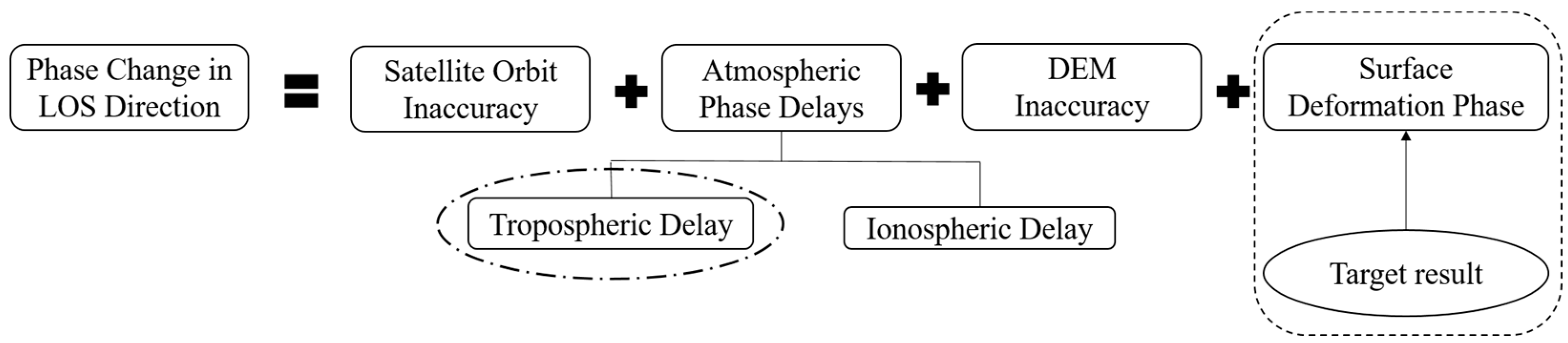
The phase changes in SAR data along the satellite line-of-sight (LOS) direction are composed of the errors in satellite orbit, the errors in the Digital Elevation Model (DEM), the atmospheric phase delay and the ground deformation-induced phase changes, as shown in Figure 1. Among these components, the ground deformation-induced phase changes are the critical data that are used to detect potential landslides. The phase changes induced by the other components should be reduced or mitigated in order to increase the measurement accuracy of InSAR. Each component is introduced as follows.

Figure 1.
Error components of interferometric phase of SAR data.
An inaccurate satellite orbit leads to errors in baseline estimation, which not only affects the removal of the flat ground phase error but also affects the calculation of the transformation parameters of the elevation and topography phase. It is a systematic error for InSAR technology. Compared with the magnitude of atmospheric phase delays, the errors induced by an inaccurate satellite orbit are insignificant [28]. The inaccurate satellite orbit could be corrected by using the more accurate orbit data provided along with the SAR images, such as the precise orbit ephemerides (POD) with a positioning accuracy of up to 5 cm.
DEM data are introduced to correct error in the topographic phase. However, these DEM data themselves may include errors. The errors in DEM data could be considered as unknown parameters, which could be solved with the technology of time series InSAR. Thus, its influence on the topographic phase could be reduced.
The atmospheric phase delay induced by a complex atmospheric environment significantly affects the measurement accuracy of InSAR [22]. Typically, the atmospheric phase delay could be divided into ionospheric delay and tropospheric delay. The ionospheric delay is induced by the variation in free electrons on the propagation path of the radar signal, and it could be decreased if smaller-wavelength SAR data (e.g., the C-band Sentinel-1A SAR data) are used [29]. The tropospheric delay is associated with spatial and temporal variation in temperature, pressure and humidity. Thus, the tropospheric delay varies significantly in different seasons.
Models have been applied to reduce the influence of the tropospheric delay. However, most applications of these models are in a time scale of year. Variations in temperature, pressure and humidity in different seasons are not considered properly. In the field of landslide detection, more accurate ground deformation is an urgent need in the rainy season in order to identify the landslide risk. As a result, it is important to investigate which model is the proper choice in different seasons. This is the motivation of this paper.
3. Main Tropospheric Correction Models
The open source program SNAP and Stanford Method for Persistent Scatters (StaMPS) are used to process the data for Persistent Scattered InSAR (PS-InSAR) [4,6]. The SAR data obtained by Sentinel-1A are used in this paper. Because the tropospheric delay is the main concern, the same orbit information and DEM data that are automatically downloaded by SNAP are used through the entire data processing. The C-band Sentinel-1A data can effectively reduce the ionospheric delay. As a result, the tropospheric delay would be the main source for the errors in the monitoring results of PS-InSAR. In order to reduce the tropospheric delay, the following four tropospheric correction models, which can be achieved in TRAIN, are selected. The applicability of these models in different seasons will be evaluated.
3.1. The Tropospheric Correction Models
Multiple tropospheric correction models have been developed to remove or mitigate the influence of the tropospheric delay to improve the accuracy of InSAR measurement. Depending on whether or not the external weather data are used, the following tropospheric correction models are selected in this paper.
3.1.1. Model A: Phase-Based Linear Model
In this model, the interferometric tropospheric phase could be calculated according to the following linear relationship:
where is the interferometric phase effected by the tropospheric delay. is a coefficient that can be calculated by the balloon sounding data. h is the elevation of the target object, which could be determined based on the DEM data. is the fixed initial phase value in the interferogram, and it is equal to the interferometric phase of PS points.
A phase-based linear model is established based on the phase and topographic information. So, it is independent of the external data or weather model. The phase-based linear model is not influenced by the external data. Therefore, it only estimates wide spatial-scale tropospheric and topography-correlated noise. The turbulent delay is not considered in this model.
3.1.2. Model B: GACOS
Generic Atmospheric Correction Online Service (GACOS), which is dependent on numerical weather models, is developed at Newcastle University [17]. GACOS can be obtained via the official website http://www.gacos.net/ (accessed on 1 August 2021) and provides a relatively independent presentation of the tropospheric delay. By implementing an iterative tropospheric decomposition model, the stratified and turbulent components are separated from tropospheric delays. Thus, Zenithal Tropospheric Delay (ZTD) maps with a high spatial resolution could be generated.
3.1.3. Model C: MERRA-2
The Modern-Era Retrospective analysis for Research Applications (MERRA-2), which was released by the NASA Global Modeling and Assimilation Office (GMAO), is selected. Unlike the above-mentioned phase-based linear method, MERRA-2 is established based on available external weather data, which include the turbulent delay.
3.1.4. Model D: Combination of MERRA-2 and Phase-Based Linear Model
Because each single model has its limitations and advantages, Bekaert [30] recommend that different correction models should be combined in a proper manner in order to effectively correct tropospheric delay. Therefore, the MERRA-2 model and phase-based linear model are combined in this paper as a comparison with the other three single models.
3.2. Evaluation of Model Applicability
The detrending standard deviation (DStd) is used to evaluate the applicability of each model mentioned above. Assuming that N pairs of SAR data are used to obtain the PS points. The earliest SAR data are assumed to be obtained at time t0, which is followed by the SAR data obtained at time t1, t2, …, tN. The ground deformation of a PS point at time ti, which is denoted as , is obtained by unwrapping the SAR data obtained at time t0 and ti. A linear function could be used to approximate the trend term of the ground deformation with time:
where is the trend term of the ground deformation. k and b are the fitting constants, which can be obtained by minimizing the sum of ( − )2 (i = 1, 2, 3, …, N).
The residual between monitored ground deformation and its trend term at time ti is expressed as follows:
The Std of the residual for a PS point, which is defined as the DStd, is expressed as follows:
where μδ is the mean value of the residuals, which is calculated as follows:
To evaluate the applicability of a tropospheric correction model, the DStd of each PS point is calculated based on the monitored ground deformation without tropospheric correction. Then, the DStds of the same PS points are calculated based on the monitored ground deformation corrected by each of the four selected tropospheric correction models. For each of the four selected tropospheric correction models, the calculated DStds of all the PS points are compared with the DStds of all the PS points without tropospheric correction. For a specific season, if a tropospheric correction model can obtain more PS points with smaller DStds than another tropospheric correction model, it means the former tropospheric correction model is less sensitive to the variation in temperature, pressure and humidity than the later tropospheric correction model. Thus, the former tropospheric correction model is more applicable than the later one in this season. In such a way, the applicability of each tropospheric correction model in different seasons could be evaluated.
4. The Framework for Selecting the Most Preferred Tropospheric Correction Model
The framework for selecting the most preferred tropospheric correction model is presented by the flowchart shown in Figure 2. This framework is illustrated in the following steps:
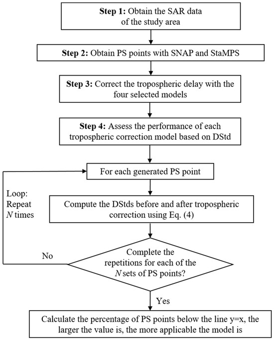
Figure 2.
The framework for selecting the proper tropospheric correction model.
Step 1: Obtain the SAR data of the study area. The Sentinel-1A SAR data are used in this paper. The data can be downloaded from https://scihub.copernicus.eu/dhus/, accessed on 15 January 2021.
Step 2: Obtain the PS points of the study area. SNAP is used to process Sentinel-1A data in order to obtain the differential interferogram. The selected public master image and the slave images are then exported to StaMPS, in which temporal processing and analysis are carried out, assuming the total number of the obtained PS points is N.
Step 3: Correct the tropospheric delay with the selected models. The phase-based linear model, MERRA-2, GACOS and the combined MERRA-2 and phase-based linear model are used in StaMPS to reduce the tropospheric delay.
Step 4: Assess the performance of each tropospheric correction model based on DStd. For each season, each of the four selected tropospheric correction models is applied to correct the tropospheric delay. Based on the DStds before and after tropospheric correction, if a tropospheric correction model can obtain more PS points with smaller DStds than another tropospheric correction model, it means the former tropospheric correction model is less sensitive to the variation in temperature, pressure and humidity than the later tropospheric correction model, and the performance of the former tropospheric correction model is better than the later one.
The proposed method and framework will be applied to a study area of Shaoxing, Zhejiang Province, China, which is introduced in the following section. This study area includes mountains and plains, which is a typical topography in Zhejiang Province. In addition, construction (e.g., subways) in this study area will be widely carried out in the future. As a result, deformation in this study area is a concern both for the government and construction companies.
5. The Application of the Proposed Method and Framework
5.1. The Study Area
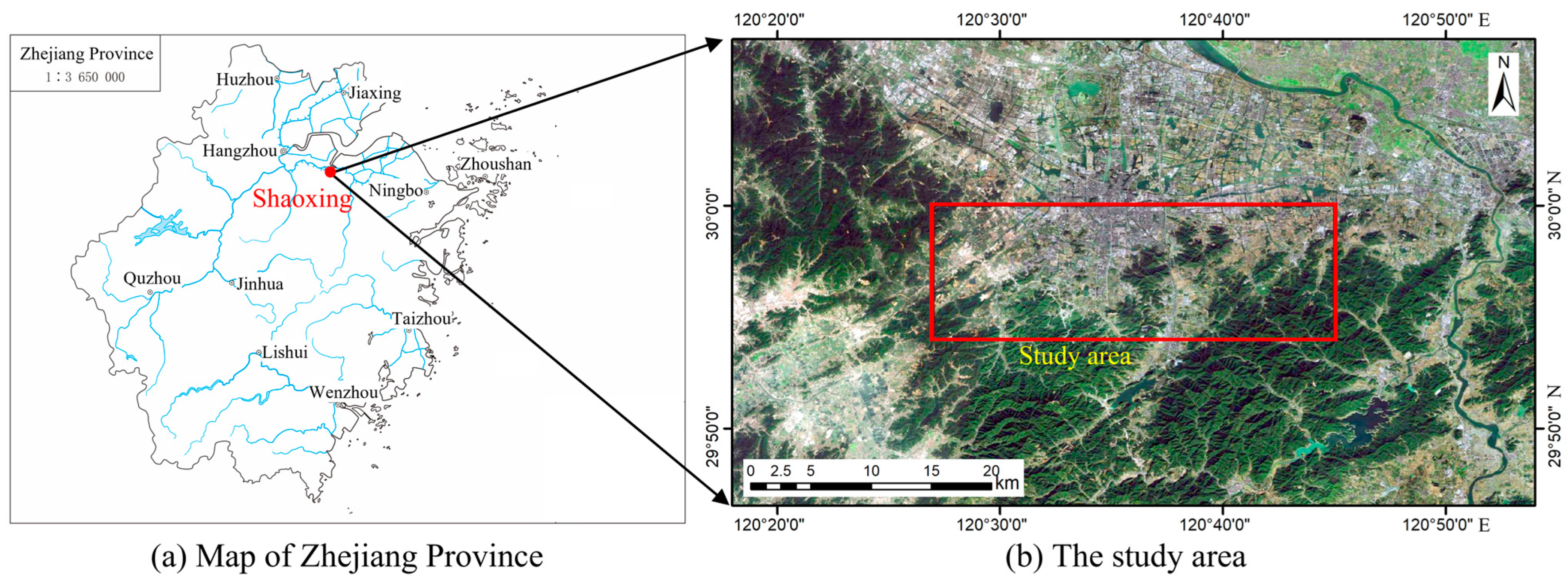
Zhejiang Province is located in the subtropical monsoon climate zone with four distinct seasons. Spring, summer, autumn and winter last from March to May, June to August, September to November and December to February of the next year, respectively. The rainy season of Zhejiang Province begins in summer and ends in early autumn. During the rainy season, landslides often occur in the mountainous region, which accounts for 70% of the total area of Zhejiang Province. Thus, there is a high demand for technology that can detect potential landslides such as PS-InSAR. A typical region of Shaoxing, which is located in the north part of Zhejiang Province, is selected as the study area, as shown in Figure 3.
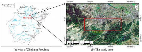
Figure 3.
The study area of Shaoxing, Zhejiang Province, China. The geographical coordinates of the study area are between 119°53′03″ E and 121°13′38″ E and 29°13′35″ N and 30°17′30″ N; mountains and plains are distributed in the south and north part of the study area. (The map of Zhejiang Province was downloaded from the website of https://zhejiang.tianditu.gov.cn/, accessed on 15 January 2021.).
5.2. The Acquisition of the SAR Data
A total of 26 C-band SAR images acquired between 31 December 2019 and 7 November 2020 by Sentinel-1A are used here. Each SAR image was acquired at 10:02 UTC time for the ascending path. The azimuth and range resolutions are 2.33 m and 13.97 m, respectively. Details of these SAR images are shown in Table 1. SRTM DEM (Digital Elevation Model, Richmond, VA, USA) data with a spatial resolution of 30 m are used to simulate the topography and ground phase in this paper. Precise orbit ephemerides (POD) with a positioning accuracy of 5 cm are applied in this case.

Table 1.
Detailed information of SAR data.
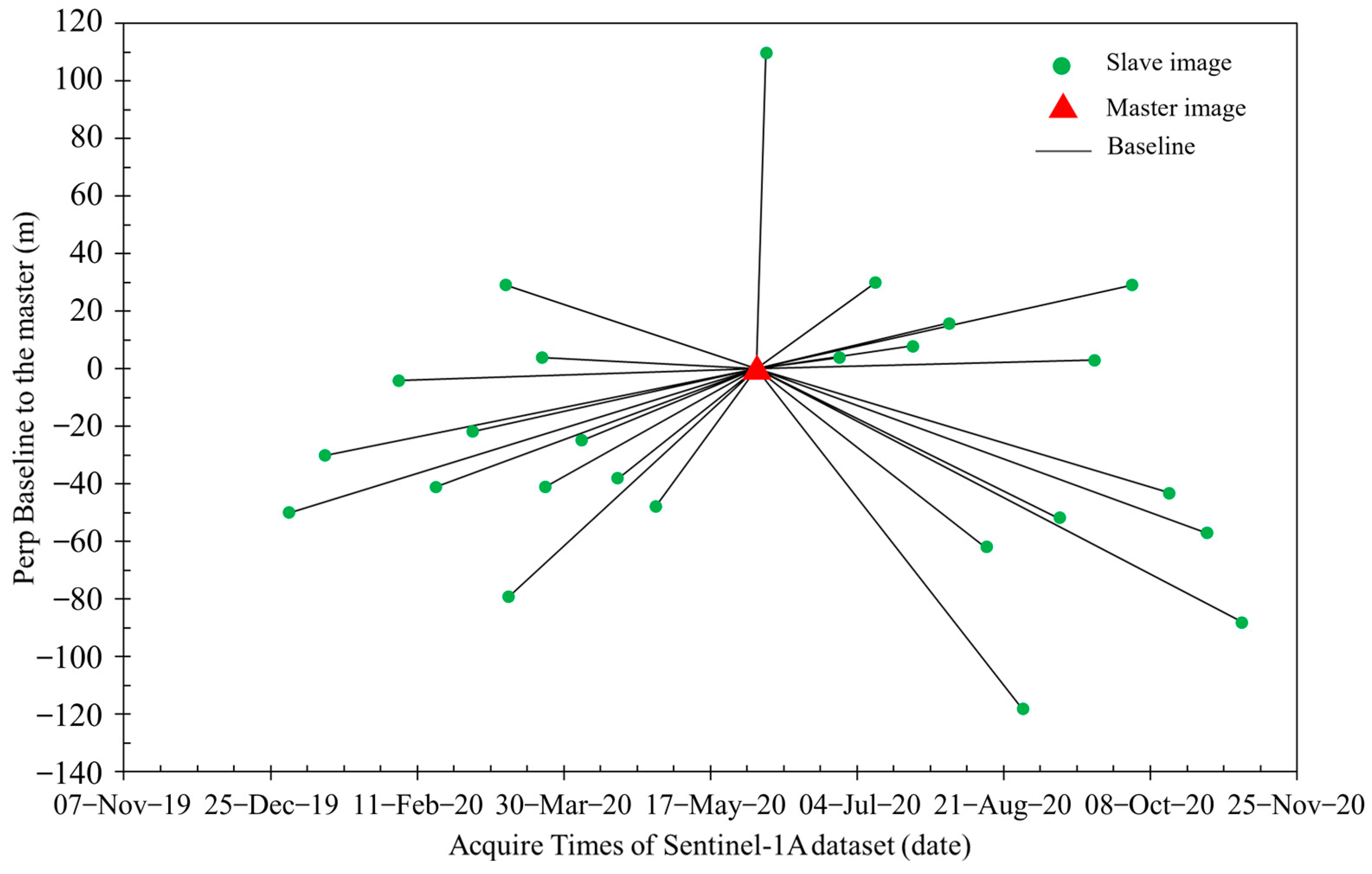
The master image has the lowest sum of the time and vertical spatial baseline, noise removal and Doppler central spectrum difference [31]. The remaining images are the slave images. The temporal and spatial baselines of the interferograms between the master and slave images are shown in Figure 4, in which the image acquired on 16 June 2020 is selected as the master image, and the remaining 25 images are the slave images.
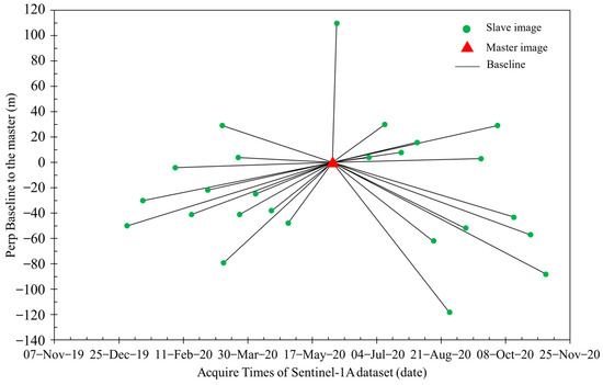
Figure 4.
Temporal and spatial baselines of the interferograms.
5.3. Results and Discussion
5.3.1. An Applicable Model over the Whole Monitoring Time Span
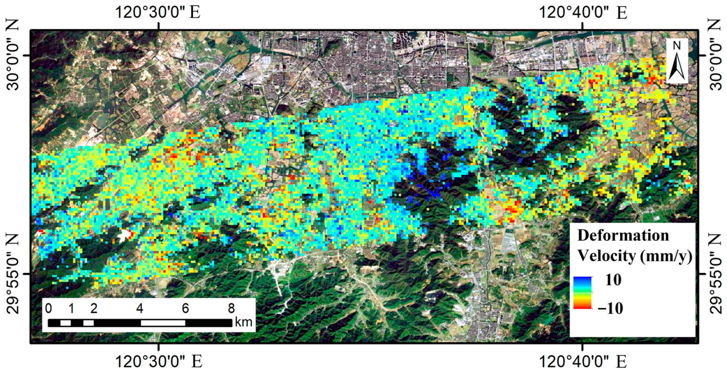
Based on the 25 interferometric pairs, 186,826 PS points are obtained in the study area. All the interferometric phases are unwrapped using the minimum cost flow method with a coherence threshold of 0.4 [32]. The PS points together with the deformation rate are imported into the remote sensing satellite image, as shown in Figure 5. Significant temporal and spatial variability in the ground deformation of the study area are observed. The maximum deformation rate is 23.8 mm/a. The distribution of ground deformation is coincident with residential area, which may be related to engineering activities and groundwater extraction. Most of the PS points are distributed on artificial buildings and bare ground. Few PS points are distributed on the area covered by forest. Such a distribution guarantees a good coherence and stability of the PS points. The maximum tropospheric delay correction values range from 5 to 25 cm for different tropospheric correction models.
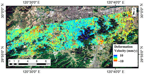
Figure 5.
The annual deformation rate of the study area (processed by PS-InSAR).
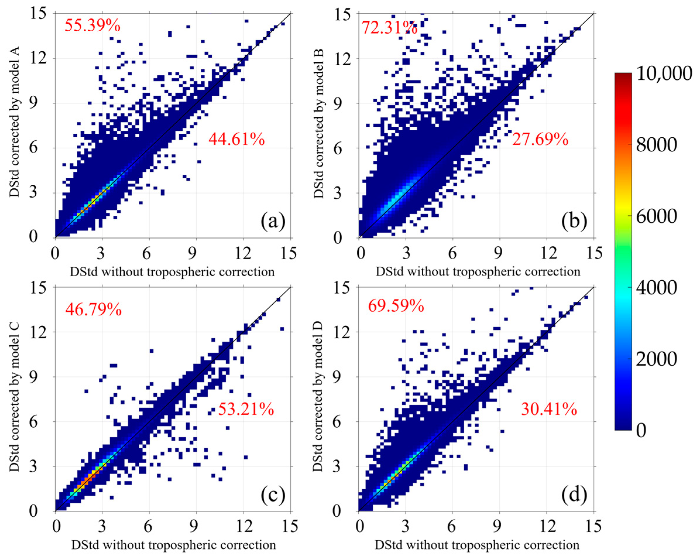
The DStds of unwrapped displacement for each PS point in the whole monitoring time span are shown in Figure 6. The color bar stands for the number of PS points. The percentages of the PS points below the line y = x (as shown in Figure 6a) for model A, B, C and D are 47.84%, 22.33%, 37.85% and 41.02%, respectively. Thus, model A, which stands for the phase-based linear model, performs better than the other three models by at least 6.6% if the whole monitoring time span of the SAR images in the study area is considered.
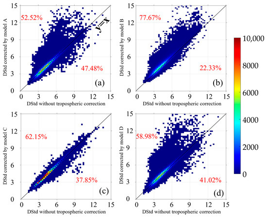
Figure 6.
The performance of each tropospheric correction model for the whole monitoring time span: (a) model A, (b) model B, (c) model C and (d) model D (the DStd is in mm).
5.3.2. Applicable Models in Different Seasons
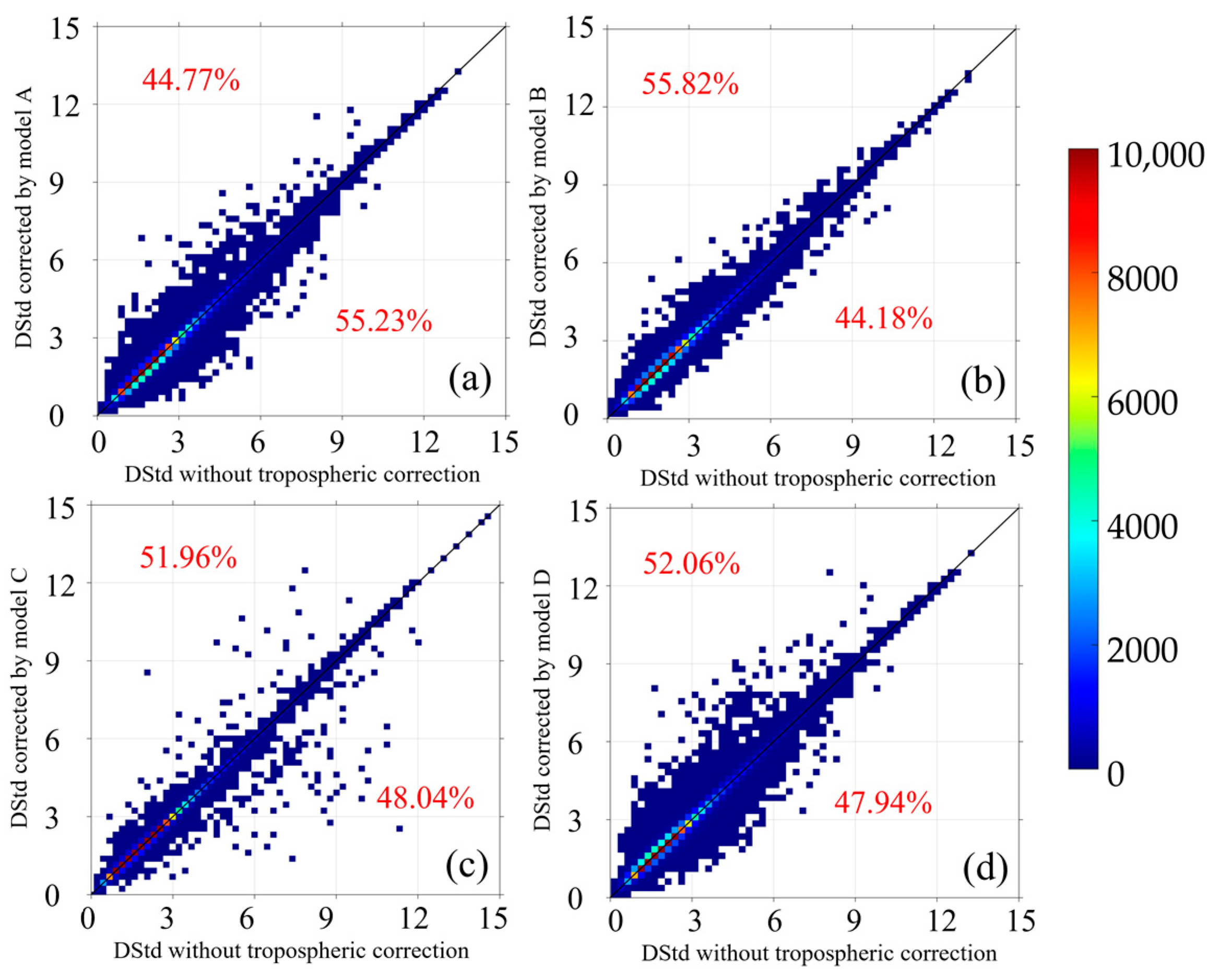
Figure 7, Figure 8, Figure 9 and Figure 10 show the DStds calculated based on the SAR data obtained in spring, summer, autumn and winter, respectively. As shown in Figure 7 and Figure 8, model C (MERRA-2) performs best among the four models. The percentages of the PS points below the line y = x corresponding to model C are 53.21% and 73.36% for spring and summer, respectively. For autumn, presented in Figure 9, model D (combination of MERRA-2 and phase-based linear model) performs the best with the percentage of the PS points below the line y = x being 50.63%. For winter, presented in Figure 10, model A (phase-based linear model) performs the best with the percentage of the PS points below the line y = x being 55.23%.

Figure 7.
The performance of each tropospheric correction model in spring: (a) model A, (b) model B, (c) model C and (d) model D (the DStd is in mm).
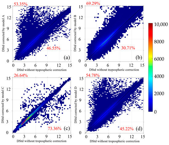
Figure 8.
The performance of each tropospheric correction model in summer: (a) model A, (b) model B, (c) model C and (d) model D (the DStd is in mm).
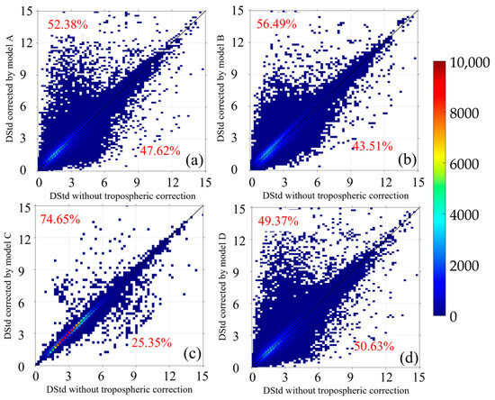
Figure 9.
The performance of each tropospheric correction model in autumn: (a) model A, (b) model B, (c) model C and (d) model D (the DStd is in mm).

Figure 10.
The performance of each tropospheric correction model in winter: (a) model A, (b) model B, (c) model C and (d) model D (the DStd is in mm).
The variation in DStds in summer and autumn is larger than that in spring and winter, which means that the tropospheric delay is more significant in summer and autumn. This is because vegetation coverage and rain are much heavier in summer and autumn than the other model in Zhejiang Province. Among the four models, model A is insensitive or robust to the variation in seasons. In spring, summer and autumn, the performance of model A (phase-based linear model) ranks in second place. In winter, model A performs the best. This is because the phase-based linear model is established based on the assumption that the relationship between the interferometric tropospheric phase and elevation is linear. No external data or errors are introduced into this model. As a result, if few data are available in a study area, the phase-based linear model might be a good choice for each season from the perspective of model robustness.
5.4. The Validation of the Performance of the Most Preferred Tropospheric Correction Model
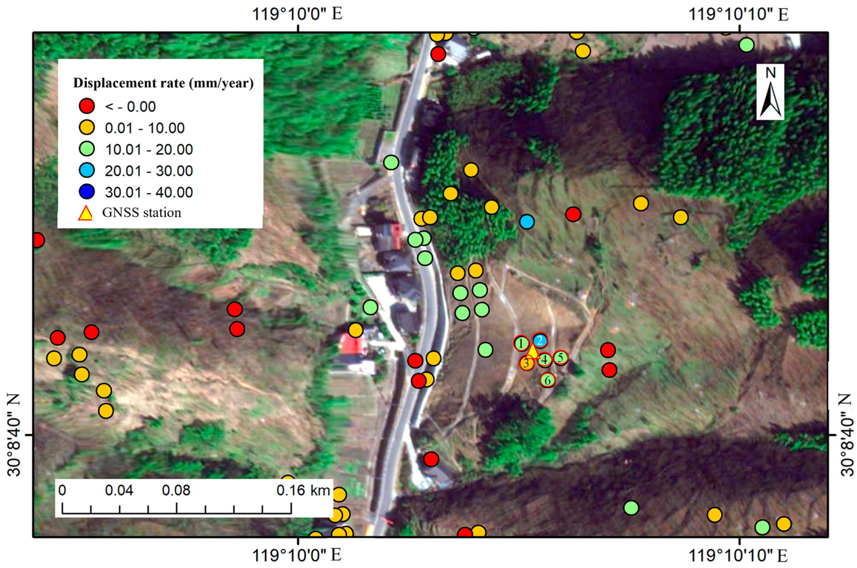
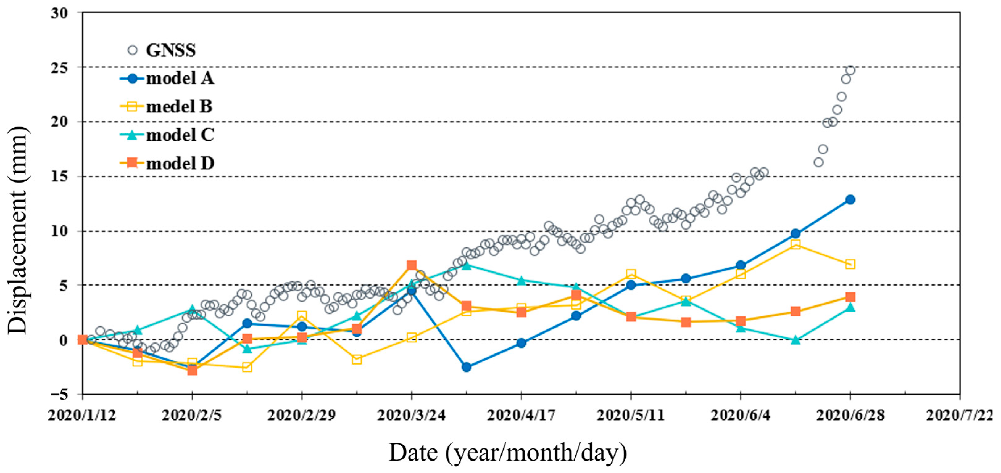
The displacement monitored by GNSS at the Changkeng landslide, which is located at Linan District, Hangzhou, Zhejiang Province, is used to validate the performance of the most preferred tropospheric correction model. Figure 11 shows the PS points and the GNSS station of the Changkeng landslide. The displacement of the PS point (NO. 1 PS point in Figure 12) that is closest to the GNSS station is used in the validation. As shown in Figure 12, the displacements monitored by PS-InSAR with model A, B, C and D are compared with the displacements monitored by GNSS. It can be seen that the displacement monitored by GNSS is larger than the displacements monitored by PS-InSAR. This is because the direction of the displacement monitored by GNSS is different from that monitored by PS-InSAR. Before 5 April 2020, the displacement rates monitored by PS-InSAR with model A, B, C and D are similar to the displacement rate monitored by GNSS. However, after 5 April 2020, only PS-InSAR with model A can capture the rapid increase in displacement that also reflects the displacement monitored by GNSS. The displacements monitored by InSAR with model B, C and D almost stay constant during this period. Thus, for the Changkeng landslide, model A performs better than the other three models.

Figure 11.
The Changkeng landslide and the distributed PS points.
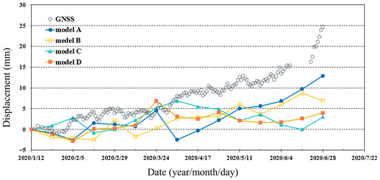
Figure 12.
Comparison of displacements between GNSS and PS-InSAR.
6. Conclusions
The applicability of the phase-based linear model, high-spatial resolution weather model (MERRA-2 and GACOS) and combination of the MERRA-2 and phase-based linear model in different seasons of Zhejiang Province is investigated and discussed. The following conclusions are obtained:
(1) The DStd of all PS points is proposed to quantify the applicability of each selected model. The influences of the atmospheric phase delay could be considered as noise in the monitoring results of InSAR. The DStd could be used to select a tropospheric correction model that is insensitive to the variations in the noise.
(2) Based on the outcome of this research, the phase-based linear model is the most proper tropospheric correction model if the whole time span of the SAR images in the study area is considered. The proper tropospheric correction model in different seasons is not the same. For spring and summer, MERRA-2 is recommended. For autumn, the combination of the MERRA-2 and phase-based linear model is recommended. For winter, the phase-based linear model is recommended.
(3) The phase-based linear model is robust against the variations in the atmospheric characteristics of the four seasons. If there are few atmospheric data available in a study area, the phase-based linear model is suggested.
(4) By comparing with displacements monitored by GNSS, it is confirmed that model A (phase-based linear model) is the best-performing model among the four selected models. InSAR with model A could capture the rapid increase in the displacement of the Changkeng landslide, which would benefit the evaluation of the potential risk of the landslide.
It should be noted that the performance of a tropospheric correction model is highly dependent on the atmospheric characteristics of a study area. This paper is preliminary research in Zhejiang Province. Further research involving other atmospheric characteristics and study areas is warranted to confirm the findings.
Author Contributions
All authors contributed to the study conception and design. Material preparation and data collection were performed by W.Z. and X.Y. Analysis was performed by Y.Y., Q.L. (Qingfang Li), Z.X. and Q.L. (Qing Lü). The first draft of the manuscript was written by Y.Y., Q.L. (Qingfang Li) and Z.X., and all authors commented on previous versions of the manuscript. All authors have read and agreed to the published version of the manuscript.
Funding
This research is financially supported by the Key R&D Project of Zhejiang Province (2021C03159) and the Natural Science Foundation of Zhejiang Province (LR24E080004), which are greatly acknowledged.
Data Availability Statement
The data presented in this study are available on request from the corresponding author.
Conflicts of Interest
The authors declare no conflicts of interest.
References
- Ferretti, A.; Prati, C.; Rocca, F. Permanent scatterers in SAR interferometry. IEEE Trans. Geosci. Remote Sens. 2001, 39, 8–20. [Google Scholar] [CrossRef]
- Berardino, P.; Fornaro, G.; Lanari, R.; Sansosti, E. A new algorithm for surface deformation monitoring based on small baseline differential SAR interferograms. IEEE Trans. Geosci. Remote Sens. 2002, 40, 2375–2383. [Google Scholar] [CrossRef]
- Mora, O.; Mallorqui, J.J.; Broquetas, A. Linear and nonlinear terrain deformation maps from a reduced set of interferometric SAR images. IEEE Trans. Geosci. Remote Sens. 2003, 41, 2243–2253. [Google Scholar] [CrossRef]
- Hooper, A.; Zebker, H.; Segall, P.; Kampes, B. A new method for measuring deformation on volcanoes and other natural terrains using InSAR persistent scatterers. Geophys. Res. Lett. 2004, 31, L23611. [Google Scholar] [CrossRef]
- Lanari, R.; Mora, O.; Manunta, M.; Mallorquí, J.J.; Berardino, P.; Sansosti, E. A small-baseline approach for investigating deformations on full-resolution differential SAR interferograms. IEEE Trans. Geosci. Remote Sens. 2004, 42, 1377–1386. [Google Scholar] [CrossRef]
- Hooper, A. A multi-temporal InSAR method incorporating both persistent scatterer and small baseline approaches. Geophys. Res. Lett. 2008, 35, L16302. [Google Scholar] [CrossRef]
- Massonnet, D.; Feigl, K.L. Radar interferometry and its application to changes in the earth’s surface. Rev. Geophys. 1998, 36, 441–500. [Google Scholar] [CrossRef]
- Cigna, F.; Osmanoğlu, B.; Cabral-Cano, E.; Dixon, T.H.; Ávila-Olivera, J.A.; Garduño-Monroy, V.H.; DeMets, C.; Wdowinski, S. Monitoring land subsidence and its induced geological hazard with synthetic aperture radar interferometry: A case study in Morelia, Mexico. Remote Sens. Environ. 2012, 117, 146–161. [Google Scholar] [CrossRef]
- Wang, T.; DeGrandpre, K.; Lu, Z.; Freymueller, J.T. Complex surface deformation of Akutan volcano, Alaska revealed from InSAR time series. Int. J. Appl. Earth Obs. Geoinf. 2018, 64, 171–180. [Google Scholar] [CrossRef]
- Hu, L.Y.; Dai, K.; Xing, C.Q.; Li, Z.H.; Tomás, R.; Clark, B.; Shi, X.L.; Chen, M.; Zhang, R.; Qiu, Q.; et al. Land subsidence in Beijing and its relationship with geological faults revealed by Sentinel-1 InSAR observations. Int. J. Appl. Earth Obs. Geoinf. 2019, 82, 101886. [Google Scholar] [CrossRef]
- Li, Y.S.; Jiao, Q.S.; Hu, X.H.; Li, Z.L.; Li, B.Q.; Zhang, J.F.; Jiang, W.L.; Luo, Y.; Li, Q.; Ba, R.J. Detecting the slope movement after the 2018 Baige Landslides based on ground-based and space-borne radar observations. Int. J. Appl. Earth Obs. Geoinf. 2020, 84, 101949. [Google Scholar] [CrossRef]
- Hooper, A.; Pietrzak, J.; Simons, W.; Cui, H.; Riva, R.; Naeije, M.; van Scheltinga, A.T.; Schrama, E.; Stelling, G.; Socquet, A. Importance of horizontal seafloor motion on tsunami height for the 2011 Mw = 9.0 Tohoku-Oki earthquake. Earth Planet. Sci. Lett. 2013, 361, 469–479. [Google Scholar] [CrossRef]
- Li, Z.; Muller, J.P.; Cross, P.; Albert, P.; Fischer, J.; Bennartz, R. Assessment of the potential of MERIS near-infrared water vapour products to correct ASAR interferometric measurements. Int. J. Remote Sens. 2006, 27, 349–365. [Google Scholar] [CrossRef]
- Ding, X.L.; Li, Z.W.; Zhu, J.J.; Feng, G.C.; Long, J.P. Atmospheric effects on InSAR measurements and their mitigation. Sensors 2008, 8, 5426–5448. [Google Scholar] [CrossRef]
- Jolivet, R.; Grandin, R.; Lasserre, C.; Doin, M.P.; Peltzer, G. Systematic InSAR tropospheric phase delay corrections from global meteorological reanalysis data. Geophys. Res. Lett. 2011, 38, L17311. [Google Scholar] [CrossRef]
- Bekaert, D.P.S.; Walters, R.J.; Wright, T.J.; Hooper, A.J.; Parker, D.J. Statistical comparison of InSAR tropospheric correction techniques. Remote Sens. Environ. 2015, 170, 40–47. [Google Scholar] [CrossRef]
- Yu, C.; Li, Z.H.; Penna, N.T.; Crippa, P. Generic atmospheric correction model for interferometric synthetic aperture radar observations. J. Geophys. Res.-Solid Earth 2018, 123, 9202–9222. [Google Scholar] [CrossRef]
- Cavalié, O.; Doin, M.P.; Lasserre, C.; Briole, P. Ground motion measurement in the Lake Mead area, Nevada, by differential synthetic aperture radar interferometry time series analysis:: Probing the lithosphere rheological structure. J. Geophys. Res.-Solid Earth 2007, 112, B03403. [Google Scholar] [CrossRef]
- Elliott, J.R.; Biggs, J.; Parsons, B.; Wright, T.J. InSAR slip rate determination on the Altyn Tagh Fault, northern Tibet, in the presence of topographically correlated atmospheric delays. Geophys. Res. Lett. 2008, 35, L12309. [Google Scholar] [CrossRef]
- Bekaert, D.P.S.; Hooper, A.; Wright, T.J. A spatially variable power law tropospheric correction technique for InSAR data. J. Geophys. Res.-Solid Earth 2015, 120, 1345–1356. [Google Scholar] [CrossRef]
- Xiao, R.Y.; Yu, C.; Li, Z.H.; He, X.F. Statistical assessment metrics for InSAR atmospheric correction: Applications to generic atmospheric correction online service for InSAR (GACOS) in Eastern China. Int. J. Appl. Earth Obs. Geoinf. 2021, 96, 102289. [Google Scholar] [CrossRef]
- Murray, K.D.; Bekaert, D.P.S.; Lohman, R.B. Tropospheric corrections for InSAR: Statistical assessments and applications to the Central United States and Mexico. Remote Sens. Environ. 2019, 232, 111326. [Google Scholar] [CrossRef]
- Abdel-Hamid, A.; Dubovyk, O.; Greve, K. The potential of sentinel-1 InSAR coherence for grasslands monitoring in Eastern Cape, South Africa. Int. J. Appl. Earth Obs. Geoinf. 2021, 98, 102306. [Google Scholar] [CrossRef]
- Scheer, J.; Caduff, R.; How, P.; Marcer, M.; Strozzi, T.; Bartsch, A.; Ingeman-Nielsen, T. Thaw-Season InSAR Surface Displacements and Frost Susceptibility Mapping to Support Community-Scale Planning in Ilulissat, West Greenland. Remote Sens. 2023, 15, 3310. [Google Scholar] [CrossRef]
- Lin, S.Y.; Chang, S.T.; Lee, C.F. InSAR-based investigation on spatiotemporal characteristics of river sediment behavior. J. Hydrol. 2023, 617, 129076. [Google Scholar] [CrossRef]
- Liu, Q.H.; Zeng, Q.M.; Zhang, Z.L. Evaluation of InSAR Tropospheric Correction by Using Efficient WRF Simulation with ERA5 for Initialization. Remote Sens. 2023, 15, 273. [Google Scholar] [CrossRef]
- Liao, M.S.; Tang, J.; Wang, T.; Balz, T.; Zhang, L. Landslide monitoring with high-resolution SAR data in the Three Gorges region. Sci. China-Earth Sci. 2012, 55, 590–601. [Google Scholar] [CrossRef]
- Fattahi, H.; Amelung, F. InSAR uncertainty due to orbital errors. Geophys. J. Int. 2014, 199, 549–560. [Google Scholar] [CrossRef]
- Gray, A.L.; Mattar, K.E.; Sofko, G. Influence of ionospheric electron density fluctuations on satellite radar interferometry. Geophys. Res. Lett. 2000, 27, 1451–1454. [Google Scholar] [CrossRef]
- Bekaert, D.P.S.; Hooper, A.; Wright, T.J. Reassessing the 2006 Guerrero slow-slip event, Mexico: Implications for large earthquakes in the Guerrero Gap. J. Geophys. Res.-Solid Earth 2015, 120, 1357–1375. [Google Scholar] [CrossRef]
- Liu, X.T.; Cao, Q.X.; Xiong, Z.G.; Wang, S.P.; Anastasia, C. Optimized method for selecting the common master image in PS-InSAR based on error analysis. J. Eng. Sci. Technol. Rev. 2018, 11, 63–71. [Google Scholar] [CrossRef]
- Eineder, M.; Hubig, M.; Milcke, B. Unwrapping large interferograms using the minimum cost flow algorithm. In Proceedings of the 1998 International Geoscience and Remote Sensing Symposium (IGARSS 98) on Sensing and Managing the Environment, Seattle, WA, USA, 10 July 1998. [Google Scholar]


Disclaimer/Publisher’s Note: The statements, opinions and data contained in all publications are solely those of the individual author(s) and contributor(s) and not of MDPI and/or the editor(s). MDPI and/or the editor(s) disclaim responsibility for any injury to people or property resulting from any ideas, methods, instructions or products referred to in the content. |
© 2024 by the authors. Licensee MDPI, Basel, Switzerland. This article is an open access article distributed under the terms and conditions of the Creative Commons Attribution (CC BY) license (https://creativecommons.org/licenses/by/4.0/).