


An Assessment of Container Seaport Efficiency Determinants


Abstract
:1. Introduction
2. Literature Review
3. Methodology
3.1. The Basics of Order-α
3.2. The Impact of Environmental Factors on Efficiency
- If ∂δ/∂Z > 0 (resp. < 0), then Z has a negative (resp. positive) effect on the attainable set [36]; similarly, in an input-oriented (resp. output-oriented) framework, if ∂Q/∂Z > 0, then Z is unfavourable (resp. favourable) to the production process, acting as an undesirable output (resp. freely available substitutive input) [32,34].
- If Δα,z= δ − δα=0.5 ≠ 0 (or ∇α,z = Q/Qα=0.5 ≠ 1), then there is a shift in the median in the efficiency distribution in addition to the full frontier shift due to factor Z [34,36]. If 0 < ∇α,z < 1, then the shift between conditional frontiers is larger than that between the unconditional ones (or in turn, the gap among the conditional and the unconditional frontiers is larger for a smaller value of α, say equal to 0.5, than for the full frontier case, α → 1). The same can be said when Δα,z > 0. On the contrary, ∇α,z > 1 and Δα,z < 0 suggest a higher efficiency spread among conditional measures [46].
4. Case Study
4.1. Seaport Sector in Europe
4.2. Data and Variables
- Inputs:
- Output:
- External/operational environment variables:
- (1)
- The sample is not uniformly distributed across those variables.
- (2)
- Landlord seaports are by far the most frequent management model in the sample. (Ports in Southern Europe do not present any other type of management model, and they constitute about half of the present set.)
- (3)
- About a third of this dataset is composed of seaports only for containers, mainly due to Southern Europe, where a quarter of them are located.
- (4)
- Most of the seaports only for containers present a landlord management model, but the reciprocal is not true.
- (5)
- Northern European countries present the highest average regional GDP.
- (6)
- It seems that landlord seaports and ports for diversified commodities are associated with the highest average regional GDP.
- (7)
- The water depth seems to be associated only with the commodity-type diversification. Greater water depths are associated with ports only for containers.
5. Results
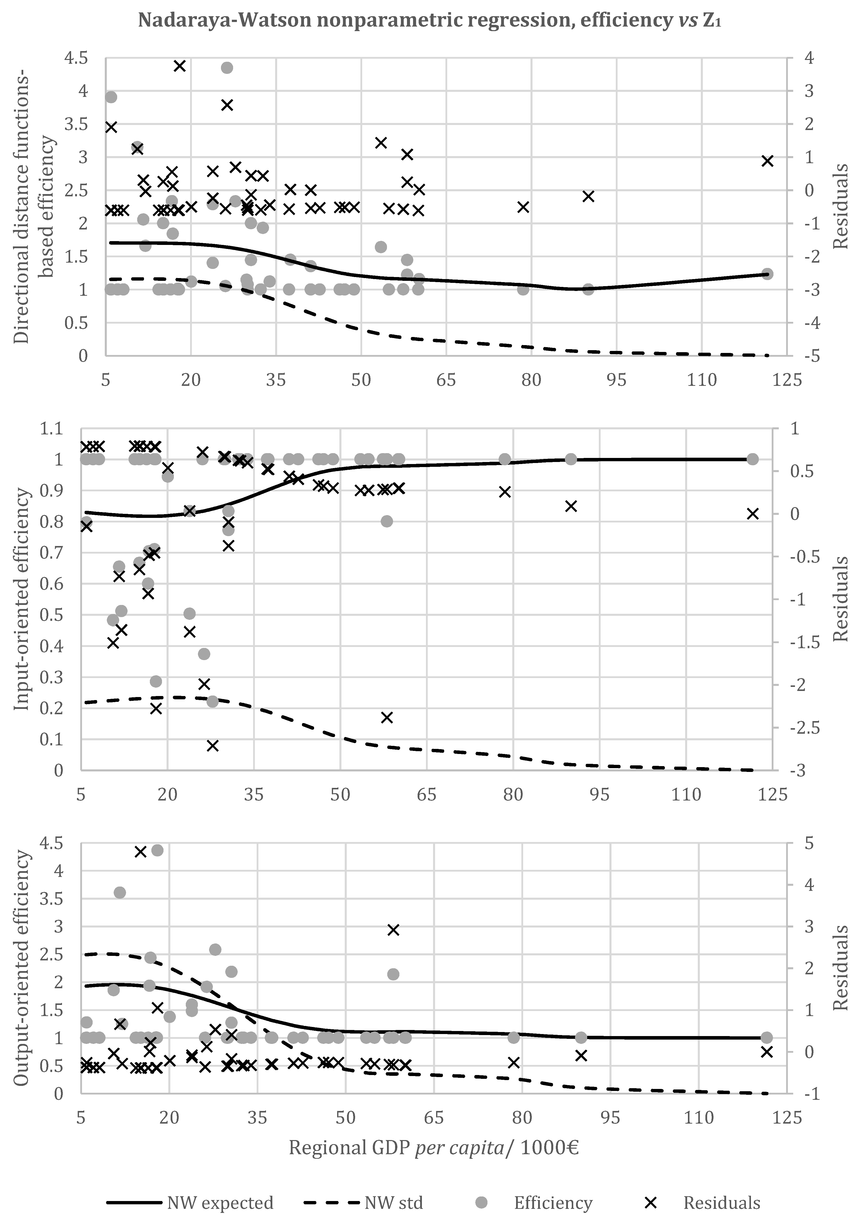
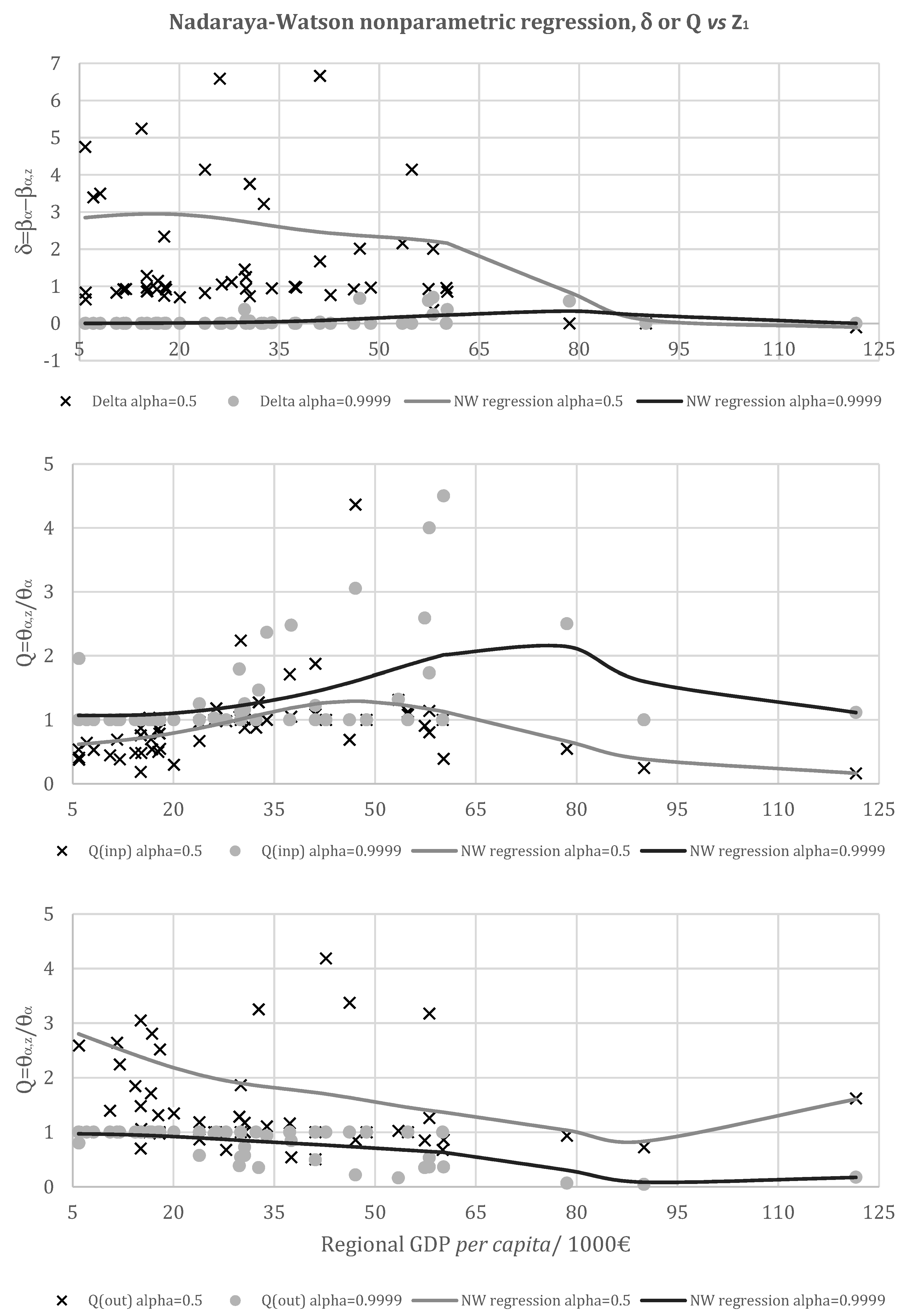
5.1. Regional GDP per Capita
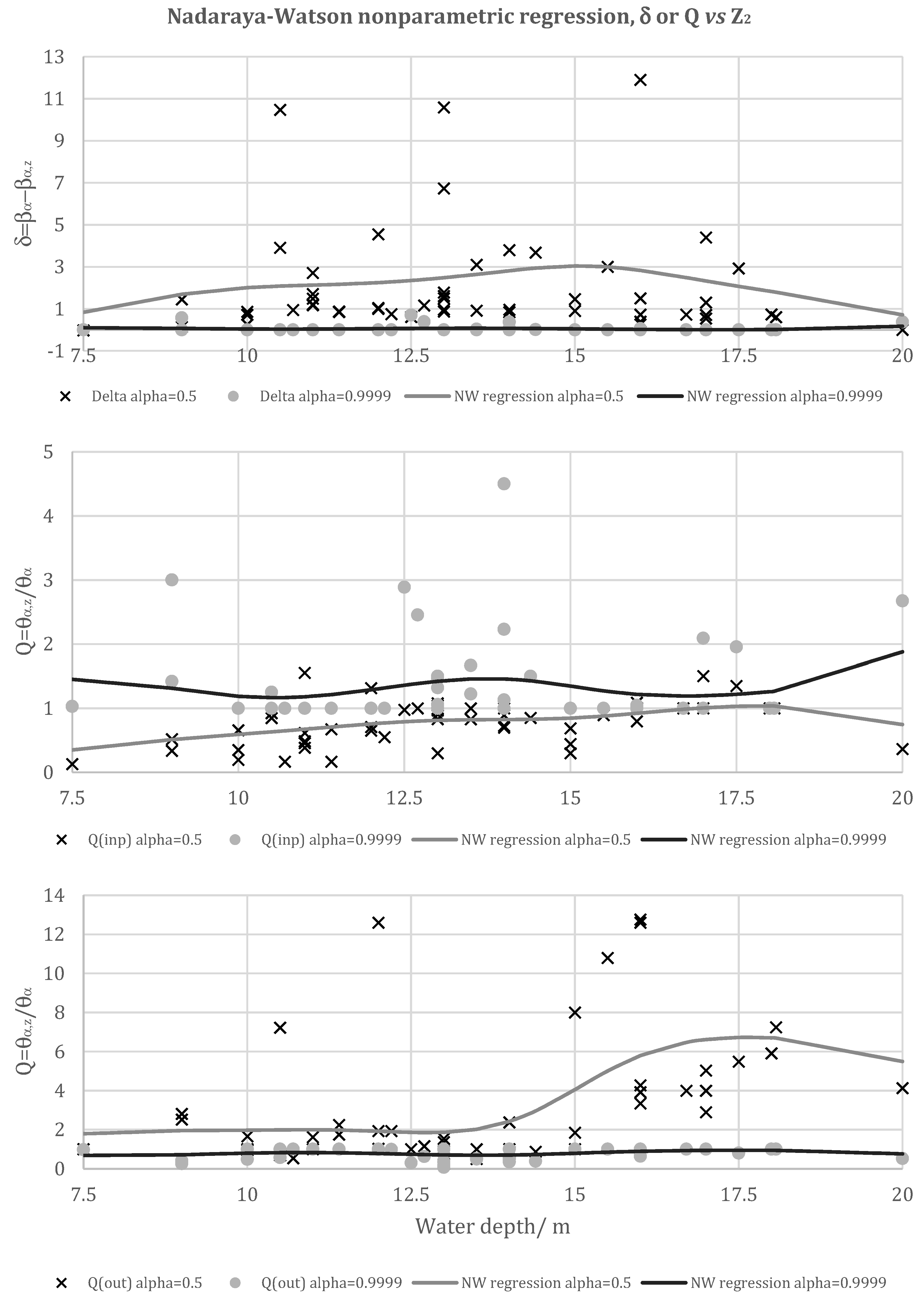
5.2. Water Depth
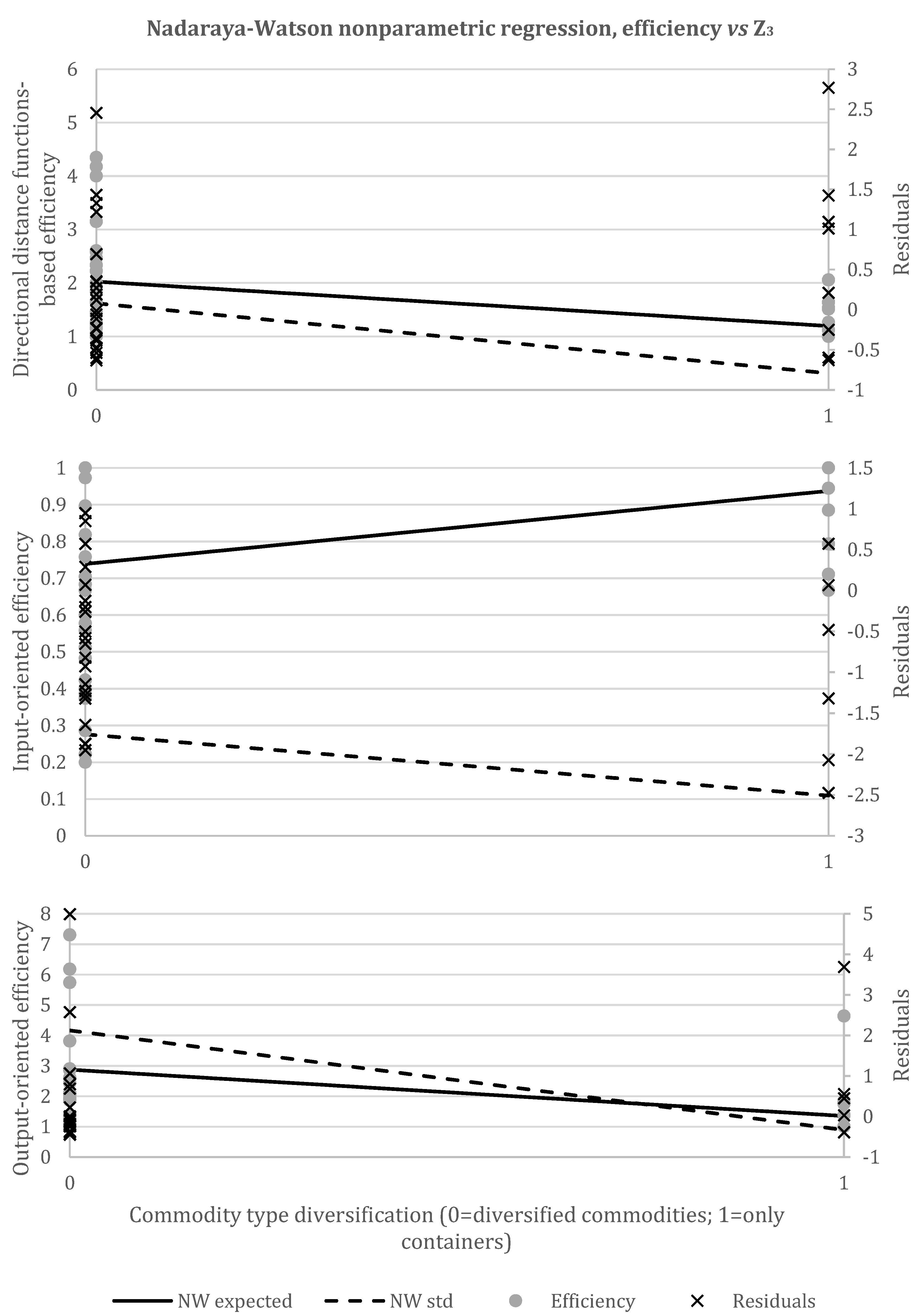
5.3. Commodity-Type Diversification
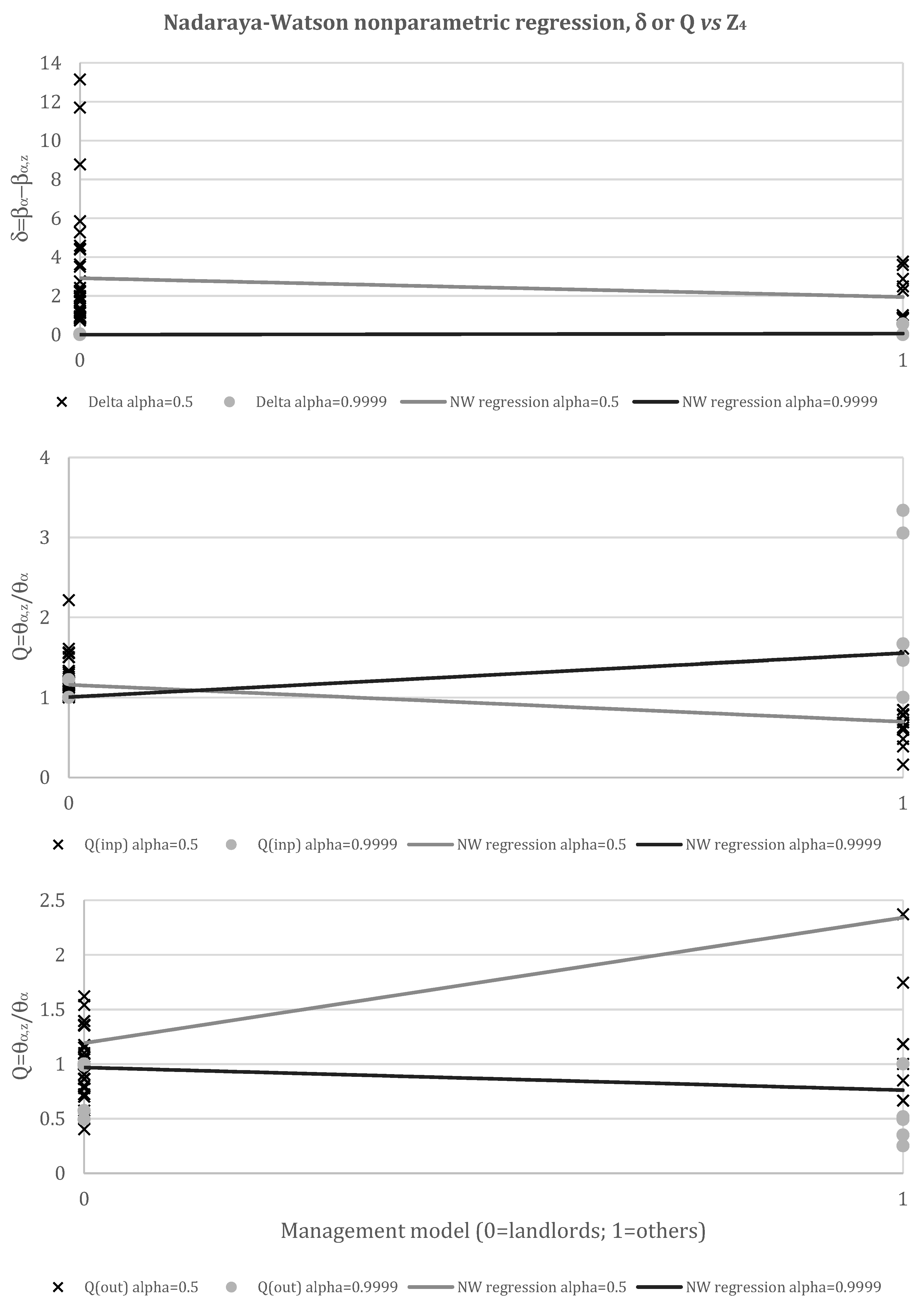
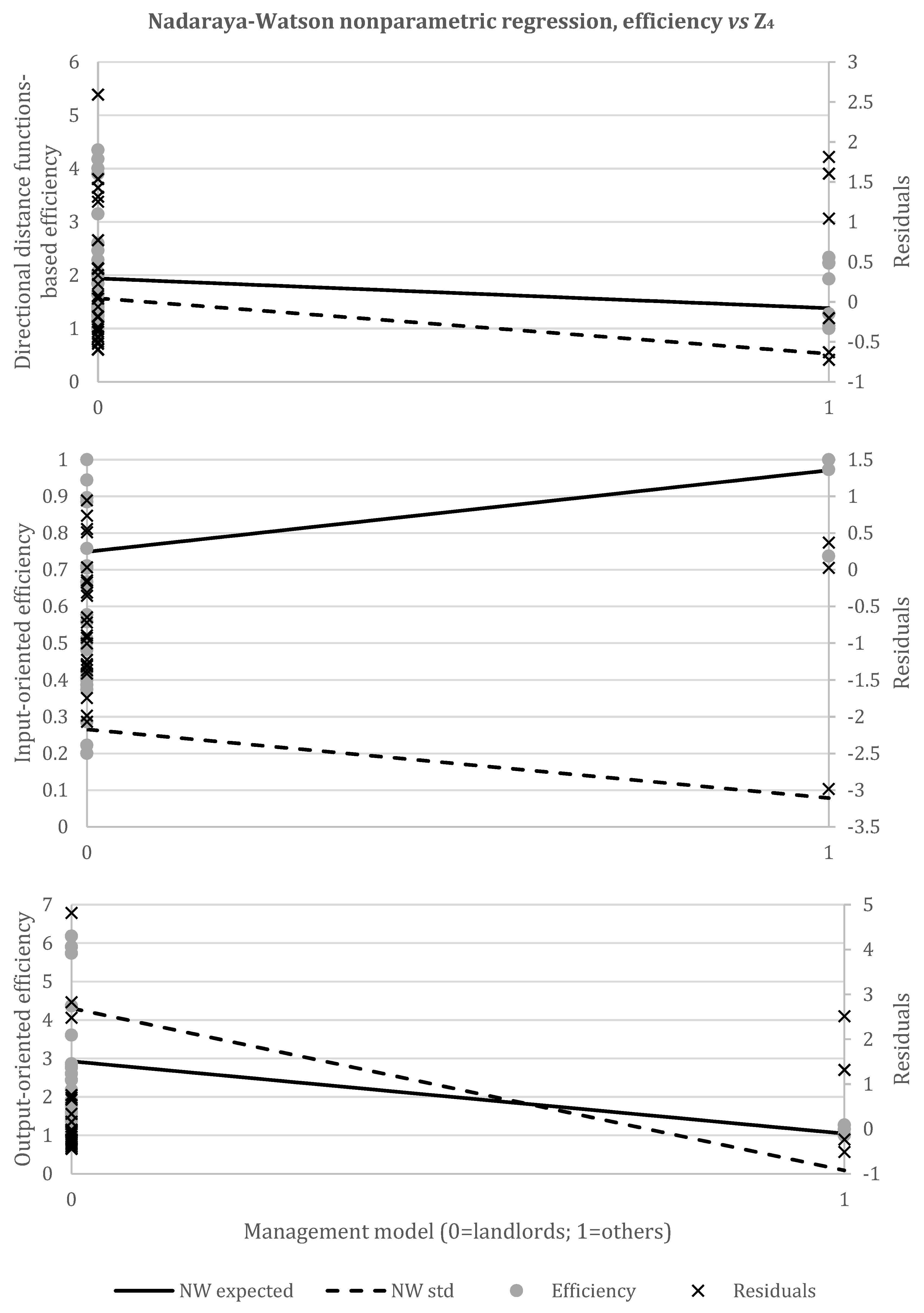
5.4. Management Model
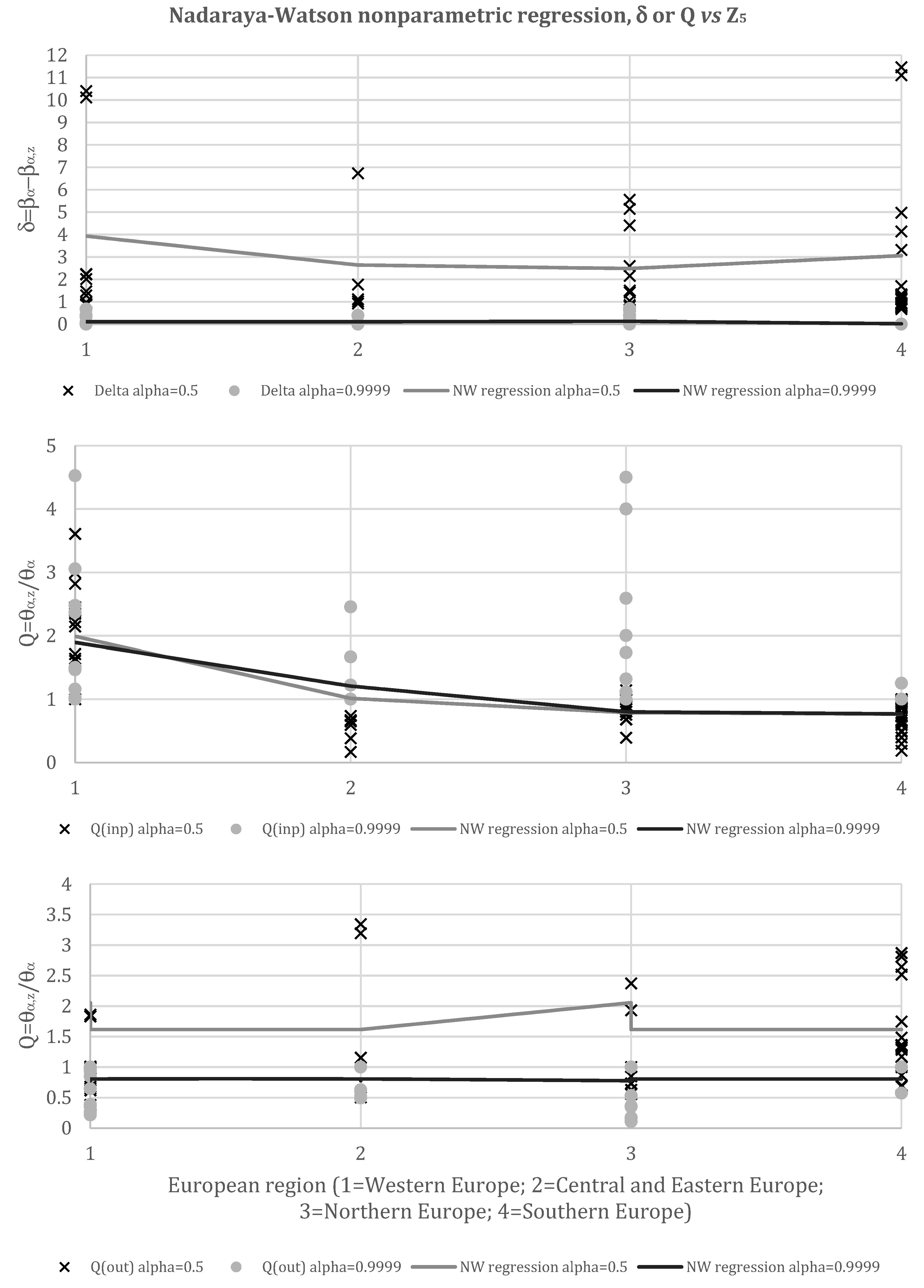
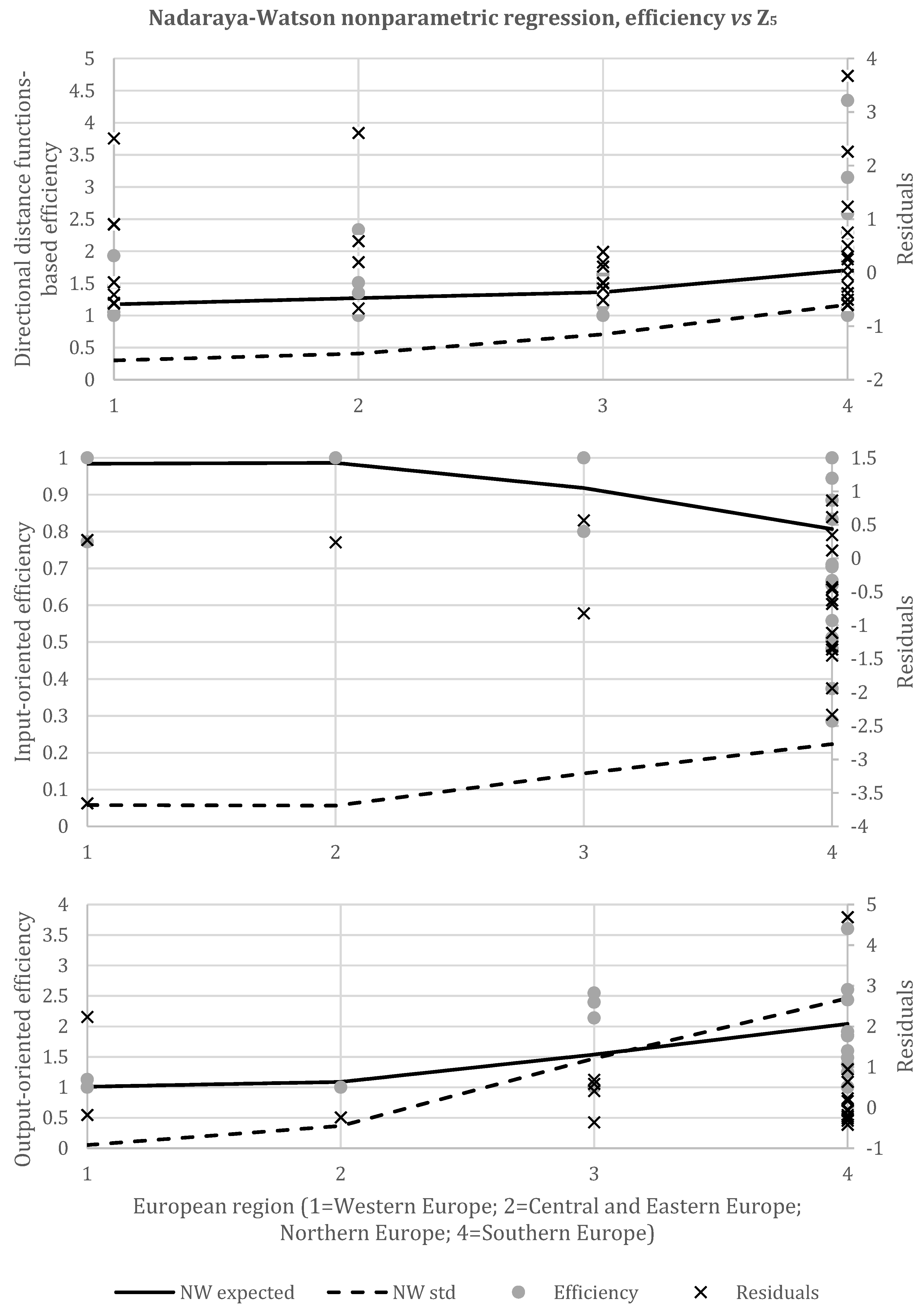
5.5. European Region
6. Discussion
7. Conclusions
Author Contributions
Funding
Institutional Review Board Statement
Informed Consent Statement
Data Availability Statement
Conflicts of Interest
Appendix A

| IV | Notes/Conclusions | ||||
|---|---|---|---|---|---|
| δ | 0.5 | D-α | −0.8773 ** | Z1 seems to have a little (meaningless) negative effect on the attainable set (AS) for seaports with Z1 ≈ 80,000 €. For smaller and larger values of Z1, technical efficiency is higher. However, this external variable presents a strong negative effect on efficiency distribution, since as Z1 decreases, δ0.5 increases. That is, smaller values of Z1 show lower values of ∆. | |
| 0.9999 | D-α | 0.8902 *** | |||
| Q | 0.5 | IO-α | 0.6652 *** | Z1 has a negative impact on the AS for values close to 80,000 €. When Z1 goes beyond (or retrograde from) that value, the technical efficiency is higher. The efficiency spread (as measured by the gap between the partial- and the full-frontier related efficiencies) is smaller for lower levels of Z1, as ∇ increases with Z1. | |
| 0.9999 | IO-α | 0.9521 *** | |||
| 0.5 | OO-α | −0.9950 ** | Z1 has a negative impact on the AS for values close to 80,000 €. When Z1 goes beyond (or retrograde from) that value, the technical efficiency is higher. The efficiency spread is higher for lower levels of Z1, as ∇ decreases with Z1, in line with the behavior of ∆. | ||
| 0.9999 | OO-α | −0.9999 ** | |||
| N.A. | D-α | 0.9353 *** | for Z1 > 78,540 €. | ||
| N.A. | IO-α | 0.6564 *** | for all values of Z1. | ||
| OO-α | −0.3102 ** | for all values of Z1. | |||
| μ | 0.9999 | D-α | −0.9949 ** | Units under larger Z1 levels are closer to the efficient frontier. | |
| 0.9999 | IO-α | 0.8660 *** | |||
| 0.9999 | OO-α | −0.9770 ** | |||
| σ | 0.9999 | D-α | −0.9757 ** | The higher Z1, the lower the technical efficiency dispersion (heteroscedasticity). | |
| 0.9999 | IO-α | −0.7279 ** | |||
| 0.9999 | OO-α | −0.9963 ** | |||
| 0.9999 | D-α | N.A. | N.A. | (positive effect as Z increases) (negative effect, meaningless though, as Z increases) | |
| 0.9999 | IO-α | N.A. | N.A. | (positive effect as Z increases) (negative effect, meaningless though, as Z increases) | |
| 0.9999 | OO-α | N.A. | N.A. | (positive effect as Z increases) (negative effect as Z increases) |
| IV | Notes/Conclusions | ||||
|---|---|---|---|---|---|
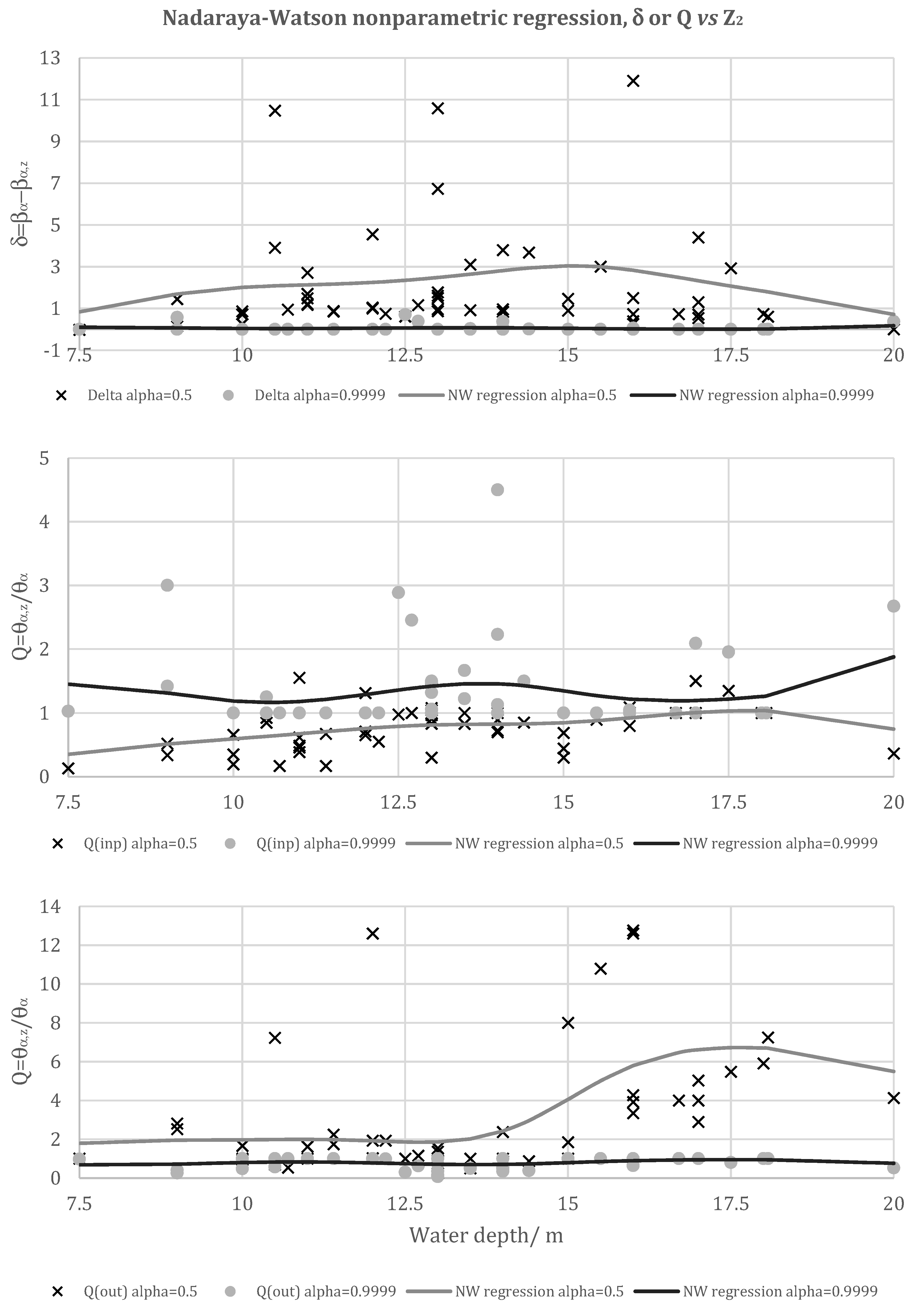
| δ | 0.5 | D-α | 0.4906 *** | Z2 has no meaningful effect on the AS. However, it seems to negatively affect the efficiency distribution since δ0.5 increases until Z2 = 16 m. | |
| 0.9999 | D-α | −0.3326 ** | |||
| Q | 0.5 | IO-α | 0.9461 *** | , Q decreases, which means that Z2 acts as a substitutive input, being conductive to efficiency; outside those ranges, its behavior seems to be the opposite. Narrower efficiency gaps occur for Z2 levels close to 10 m and 17.5 m. | |
| 0.9999 | IO-α | 0.2479 * | |||
| 0.5 | OO-α | 0.7590 *** | Z2 has no meaningful effect on the AS. However, it seems to negatively affect the efficiency distribution since δ0.5 increases until Z2 = 17.5 m. Seaports with water depth between 7.5 and 13 m present lower levels of efficiency spread. | ||
| 0.9999 | OO-α | 0.3754 *** | |||
| N.A. | D-α | −0.2970 ** | for all values of Z2. | ||
| N.A. | IO-α | −0.6452 ** | for all values of Z2. | ||
| OO-α | −0.8967 ** | ||||
| μ | 0.9999 | D-α | −0.9503 ** | Units under larger Z2 levels are closer to the efficient frontier. | |
| 0.9999 | IO-α | 0.5203 *** | |||
| 0.9999 | OO-α | −0.9069 ** | |||
| σ | 0.9999 | D-α | −0.8930 ** | The higher Z2, the lower the technical efficiency dispersion (heteroscedasticity). | |
| 0.9999 | IO-α | −0.4911 ** | |||
| 0.9999 | OO-α | −0.9400 ** | |||
| 0.9999 | D-α | N.A. | N.A. | (negative effect as Z increases) (positive effect as Z increases) (negative effect as Z increases) | |
| 0.9999 | IO-α | N.A. | N.A. | (positive effect as Z increases) (positive effect as Z increases) (negative effect as Z increases) | |
| 0.9999 | OO-α | N.A. | N.A. | (positive effect as Z increases) (negative effect as Z increases) (negative effect, meaningless though, as Z increases) |
| Reference Group | D-α | IO-α | OO-α |
|---|---|---|---|
| 1—Western Europe | |||
| 2—Central and Eastern Europe | |||
| 3—Northern Europe | |||
| 4—Southern Europe |

References
- Oliveira, L. Portugal na rede transeuropeia, contexto histórico e objetivos actuais, o que falta fazer? Portugal 2020. Rev. Cient. Ingenium 2015, 2, 22. [Google Scholar]
- Talley, W.K.; Ng, M.; Marsillac, E. Port service chains and port performance evaluation. Transp. Res. Part E 2014, 69, 236–247. [Google Scholar] [CrossRef]
- Lam, J.S.L.; Gu, Y. A market-oriented approach for intermodal net work optimisation meeting cost, time and environmental requirements. Int. J. Prod. Econ. 2016, 171, 266–274. [Google Scholar] [CrossRef]
- European Union. The World Factbook; Factbook, CIA World: Langley, VA, USA, 2014. [Google Scholar]
- Simões, P.; Marques, R. Seaport performance analysis by robust non-parametric efficient estimators. Transp. Plan. Technol. 2010, 33, 435–451. [Google Scholar] [CrossRef]
- Tongzon, J.; Heng, W. Port privatization, efficiency and competitiveness: Some empirical evidence from container ports (terminals). Transp. Res. Part A 2005, 39, 405–424. [Google Scholar] [CrossRef]
- Chang, V.; Tovar, B. Drivers explaining the inefficiency of Peruvian and Chilean ports terminals. Transp. Res. Part E: Logist. Transp. Rev. 2014, 67, 190–203. [Google Scholar] [CrossRef]
- Aragon, Y.; Daouia, A.; Thomas-Agnan, C. Nonparametric frontier estimation: A conditional quantile-based approach. Econom. Theory 2005, 21, 358–389. [Google Scholar] [CrossRef]
- Wang, T.; Song, D.; Cullinane, K. Container port production efficiency: A comparative study of DEA and FDH approaches. J. East. Asia Soc. Transp. Stud. 2003, 5, 698–713. [Google Scholar]
- Cullinane, K.; Wang, T.; Song, D.; Ji, P. The technical efficiency of container ports: Comparing data envelopment analysis and stochastic frontier analysis. Transp. Res. Part A 2006, 40, 354–374. [Google Scholar] [CrossRef]
- Munisamy, S.; Singh, G. Benchmarking the Efficiency of Asian Container Ports. Afr. J. Bus. Manag. 2011, 5, 1397–1407. [Google Scholar]
- Lu, B.; Wang, X. Application of DEA on the measurement of operating efficiencies for east-Asia major container terminals. J. Syst. Manag. Sci. 2012, 2, 1–18. [Google Scholar]
- Merk, O.; Dang, T. Efficiency of world ports in container and bulk cargo (oil, coal, ores and grain). In OECD Regional Development Working Papers; OECD Publishing: Paris, France, 2012. [Google Scholar]
- Lu, B.; Park, N. Sensitivity analysis for identifying the critical productivity factors of container terminals. J. Mech. Eng. 2013, 59, 536–546. [Google Scholar] [CrossRef]
- Mokhtar, K.; Shah, M. Efficiency of operations in container terminals: A Frontier Method. Eur. J. Bus. Manag. 2013, 5, 91–106. [Google Scholar]
- Tongzon, J. Efficiency measurement of selected Australian and other international ports using data envelopment analysis. Transp. Res. Part A 2001, 35, 107–122. [Google Scholar] [CrossRef]
- Lin, L.; Tseng, L. Application of DEA and SFA on the measurement of operating efficiencies for 27 international container ports. Proc. East. Asia Soc. Transp. Stud. 2005, 5, 592–607. [Google Scholar]
- Wang, T.; Cullinane, K. The efficiency of European container terminals and implications for supply chain management. Marit. Econ. Logist. Palgrave Macmillan 2006, 8, 8299. [Google Scholar] [CrossRef]
- Al-Eraqi, A.; Mustaffa, A.; Khader, A.; Barros, C. Efficiency of Middle Eastern and East African Seaports: Application od DEA using window analysis. Eur. J. Sci. Res. 2008, 23, 597–612. [Google Scholar]
- Munisamy, S.; Jun, O. Efficiency of Latin American container seaports using DEA. In Proceedings of the 3rd Asia-Pacific Business Research Conference, Kuala Lumpur, Malaysia, 25–26 February 2013. [Google Scholar]
- Shin, C.; Jeong, D. Data envelopment analysis for container terminals considering an undesirable output-Focus on Busan Port & Kwangyang Port. J. Navig. Port Res. 2013, 37, 195–201. [Google Scholar]
- Wanke, P.; Barros, C. Public-Private Partnerships and Scale Efficiency in Brazilian Ports: Evidence from Two-Stage DEA Analysis. Socio-Econ. Plan. Sci. 2015, 51, 13–22. [Google Scholar] [CrossRef]
- Marques, R.; Carvalho, M. Governance and performance evaluation of the Portuguese seaports in the European context. Int. J. Serv. Econ. Manag. 2009, 1, 340–357. [Google Scholar] [CrossRef]
- Barros, C. A benchmark analysis of Italian seaports using data envelopment analysis. Marit. Econ. Logist. 2006, 8, 347–365. [Google Scholar] [CrossRef]
- Nigra, S. Efficiency of the Seaport Sector. Master’s Thesis, Universidade Técnica de Lisboa, Lisbon, Portugal, 2010. [Google Scholar]
- Pjevčević, D.; Radonjić, A.; Hrle, Z.; Promet, Č. DEA Window Analysis for Measuring Port Efficiencies in Serbia. Traffic Transp. 2012, 24, 63–72. [Google Scholar] [CrossRef]
- Wanke, P. Physical infrastructure and shipment consolidation efficiency drivers in Brazilian ports: A two-stage network-DEA approach. Transp. Policy 2013, 29, 145–153. [Google Scholar] [CrossRef]
- Wilmsmeier, G.; Tovar, B.; Sanchez, R. The evolution of container terminal productivity and efficiency under changing economic environments. Res. Transp. Bus. Manag. 2013, 8, 50–66. [Google Scholar] [CrossRef]
- Cullinane, K.; Wang, T. The efficiency analysis of container port production using DEA panel data approaches. OR Spectr. 2010, 32, 717–738. [Google Scholar] [CrossRef]
- Badin, L.; Daraio, C.; Simar, L. How to measure the impact of environmental factors in a nonparametric production model. Eur. J. Oper. Res. 2012, 223, 818–833. [Google Scholar] [CrossRef]
- Hirschberg, J.G.; Lloyd, P.J. Does the technology of foreign-invested enterprises spill over to other enterprises in china? An application of post-DEA bootstrap regression analysis. In Modelling the Chinese Economy; Lloyd, P.J., Zang, X.G., Eds.; Edward Elgar Press: London, UK, 2002. [Google Scholar]
- Daraio, C.; Simar, L. Advanced robust and nonparametric methods in efficiency analysis. In Series: Studies in Productivity and Efficiency; Springer: Berlin/Heidelberg, Germany, 2007. [Google Scholar]
- Simar, L.; Wilson, P. Estimation and inference in two-sage semi-parametric models of production processes. J. Econom. 2007, 136, 31–64. [Google Scholar] [CrossRef]
- Ferreira, D.C.; Figueira, J.R.; Greco, S.; Marques, R.C. Data envelopment analysis models with imperfect knowledge of input and output values: An application to Portuguese public hospitals. Expert Syst. Appl. 2023, 231, 120543. [Google Scholar] [CrossRef]
- Cazals, C.; Florens, J.; Simar, L. Nonparametric frontier estimation: A robust approach. J. Econom. 2002, 106, 1–25. [Google Scholar] [CrossRef]
- Daraio, C.; Simar, L. Directional distances and their robust versions: Computational and testing issues. Eur. J. Oper. Res. 2014, 237, 358–369. [Google Scholar] [CrossRef]
- Simar, L.; Wilson, P. Statistical inference in non-parametric frontier models: The state of the art. J. Product. Anal. 2003, 13, 49–78. [Google Scholar] [CrossRef]
- Simar, L.; Wilson, P. Two-stage DEA: Caveat emptor. J. Product. Anal. 2011, 36, 205–218. [Google Scholar] [CrossRef]
- Badin, L.; Daraio, C.; Simar, L. Optimal bandwidth selection for conditional efficiency measures: A data-driven approach. Eur. J. Oper. Res. 2010, 201, 640–663. [Google Scholar] [CrossRef]
- Daraio, C.; Simar, L. Introducing environmental variables in nonparametric frontier models: A probabilistic approach. J. Product. Anal. 2005, 24, 93–121. [Google Scholar] [CrossRef]
- Chambers, R.G.; Chung, Y.; Färe, R. Profit, Directional Distance Functions, and Nerlovian Efficiency. J. Optim. Theory Appl. 1998, 98, 351–364. [Google Scholar] [CrossRef]
- Färe, R.; Grosskopf, S.; Lovell, K.A. The Measurement of Efficiency of Production; Kluwer Nijhof Publishing: Boston, MA, USA, 1985. [Google Scholar]
- Simar, L.; Vanhems, A. Probabilistic characterization of directional distances and their robust versions. J. Econom. 2012, 166, 342–354. [Google Scholar] [CrossRef]
- Ferreira, D.C.; Marques, R.C. A step forward on order-α robust nonparametric method: Inclusion of weight restrictions, convexity and non-variable returns to scale. Oper. Res. 2020, 20, 1011–1046. [Google Scholar] [CrossRef]
- Ferreira, D.C.; Marques, R.C.; Nunes, A.M. Economies of scope in the health sector: The case of Portuguese hospitals. Eur. J. Oper. Res. 2018, 266, 716–735. [Google Scholar] [CrossRef]
- Ibrahim, M.D.; Alola, A.A.; Ferreira, D.C. Assessing sustainable development goals attainment through energy-environmental efficiency: The case of Latin American and Caribbean countries. Sustain. Energy Technol. Assess. 2023, 57, 103219. [Google Scholar] [CrossRef]
- Simões, P.; Marques, R. Influence of congestion efficiency on the European seaports performance. Does it matter? Transp. Rev. 2010, 30, 517–539. [Google Scholar] [CrossRef]
- Portopia. European Port Industry Sustainability Report 2016; The European Sea Ports Organisation: Bruxelles, Belgium, 2016. [Google Scholar]
- Carvalho, P.; Marques, R. Using non-parametric technologies to estimate returns to scale in the Iberian and international seaports. Int. J. Shipp. Transp. Logist. 2012, 4, 286–302. [Google Scholar] [CrossRef]
- Bichou, K. An empirical study of the impacts of operating and market conditions on container-port efficiency and benchmarking. Res. Transp. Econ. 2013, 42, 2837. [Google Scholar] [CrossRef]
- Liu, Q. Efficiency Analysis of Container Ports and Terminals. Ph.D. Thesis, Philosophy of University College London, London, UK, 2010. [Google Scholar]
- Caldeirinha, V.; Felicio, J.; Dionisio, A. Effect of the Container Terminal Characteristics on Performance; CEFAGE-UE Working Paper; University of Evora: Évora, Portugal, 2013; pp. 1–18. [Google Scholar]
- Levinson, M. Freight pain: The rise and fall of globalization. Foreign Aff. 2008, 87, 133140. [Google Scholar]
- Trujillo, L.; Tovar, B. The European Port Industry: An Analysis of its Economic Efficiency. Marit. Econ. Logist. 2007, 9, 148–171. [Google Scholar] [CrossRef]
- Li, K.; Cheng, L. The determinants of maritime policy. Marit. Policy Manag. 2007, 34, 521–533. [Google Scholar] [CrossRef]
- Giuffrida, A.; Gravelle, H. Measuring Performance in Primary Care: Econometric Analysis and DEA. J. Appl. Econ. 2001, 33, 163–175. [Google Scholar] [CrossRef]
- Oliveira, R.; Pedro, M.; Marques, R. Efficiency and its Determinants in Portuguese Hotels in the Algarve. Tour. Manag. 2013, 36, 641–649. [Google Scholar] [CrossRef]
- Simar, L.; Zelenyuk, V. On Testing Equality of Distributions of Technical Efficiency Scores. Econom. Rev. 2006, 25, 497–522. [Google Scholar] [CrossRef]
- Lun, Y.V.; Shang, K.C.; Lai, K.H.; Cheng, T.C.E. Examining the influence of organizational capability in innovative business operations and the mediation of profitability on customer satisfaction: An application in intermodal transport operators in Taiwan. Int. J. Prod. Econ. 2016, 171, 179–188. [Google Scholar] [CrossRef]
- Niavis, S.; Tsekeris, T. Ranking and causes of inefficiency of container seaports in South-Eastern Europe. Eur. Transp. Res. Rev. 2012, 4, 235–244. [Google Scholar] [CrossRef]
- Coto-Millan, P.; Banos-Pino, J.; Rodriguez-Alvarez, A. Economic efficiency in Spanish ports: Some empirical evidence. Marit. Policy Manag. 2000, 27, 169–174. [Google Scholar] [CrossRef]
- Ferreira, D.C.; Marques, R.C. Identifying congestion levels, sources and determinants on intensive care units: The Portuguese case. Health Care Manag. Sci. 2016, 21, 348–375. [Google Scholar] [CrossRef] [PubMed]
- Ferreira, D.C.; Marques, R.C. Did the corporatization of Portuguese hospitals significantly change their productivity? Eur. J. Health Econ. 2015, 16, 289–303. [Google Scholar] [CrossRef] [PubMed]
- Ferreira, D.C.; Marques, R.C. Should inpatients be adjusted by their complexity and severity for efficiency assessment? Evidence from Portugal. Health Care Manag. Sci. 2016, 19, 43–57. [Google Scholar] [CrossRef] [PubMed]
- Ferreira, D.C.; Marques, R.C. Do quality and access to hospital services impact on their technical efficiency? Omega 2019, 86, 218–236. [Google Scholar] [CrossRef]
- Ibrahim, M.D.; Ferreira, D.C.; Daneshvar, S.; Marques, R.C. Transnational resource generativity: Efficiency analysis and target setting of water, energy, land, and food nexus for OECD countries. Sci. Total Environ. 2019, 697, 134017. [Google Scholar] [CrossRef] [PubMed]
- Ferreira, D.C.; Caldas, P.; Varela, M.; Marques, R.C. A geometric aggregation of performance indicators considering regulatory constraints: An application to the urban solid waste management. Expert Syst. Appl. 2023, 218, 119540. [Google Scholar] [CrossRef]
- Amaral, C.; Pedro, M.I.; Ferreira, D.C.; Marques, R.C. Performance and its determinants in the Portuguese municipal solid waste utilities. Waste Manag. 2022, 139, 70–84. [Google Scholar] [CrossRef] [PubMed]
- Ferreira, D.C.; Marques, R.C.; Pedro, M.I. Comparing efficiency of holding business model and individual management model of airports. J. Air Transp. Manag. 2016, 57, 168–183. [Google Scholar] [CrossRef]
- Ferreira, D.C.; Marques, R.C.; Pedro, M.I. Explanatory variables driving the technical efficiency of European seaports: An order-α approach dealing with imperfect knowledge. Transp. Res. Part E Logist. Transp. Rev. 2018, 119, 41–62. [Google Scholar] [CrossRef]

| Authors | Sample | Methodology | Variables Input/Output | Main Conclusions |
|---|---|---|---|---|
| Simões and Marques [5] | 41 seaports in 11 European countries | DEA FDH Order-m | Input: total expenses Output: container, dry bulk cargo, liquid bulk cargo and passengers | Considerable levels of inefficiency were found in the European seaports sector. A significant portion of inefficiency is caused by scale diseconomies. This means that European seaports could save on average 22.2% of the inputs consumed if they operated at an optimal scale. |
| Chang and Tovar [7] | 14 terminals in Peru and Chile (2004–2010) | SFA | Input: capital, labour, bulk rate, containerisation rate, occupancy rate Output: containers, general and rolling freight, bulk | Chilean terminals were more efficient than the Peruvian ones, mainly due to greater agility in the implementation of the reform process. Furthermore, the higher the containerisation index, the greater the occupancy rate and the bigger the bulk rate, then the lower the inefficiency in terminals is. Also, the inefficiency is lower when the terminal is under private administration. |
| Wang, Song and Cullinane [9] | 57 international ports/terminals (2001) | DEABCC, DEACCR and FDH | Input: quay length, terminal area, quayside gantry, yard gantry, straddle carrier Output: container throughput | The results found that some renowned container terminals, such as MTL in Hong Kong, are currently suffering from inefficient production. On the basis of using cross-sectional data, however, this inefficiency could very likely be caused by a recent investment in future production. |
| Cullinane, Wang, Song and Ji [10] | 57 international ports/terminals (2001) (2001) | DEA and SFA | Input: quay length, terminal area, quayside gantry, yard gantry, straddle carrier Output: container throughput | High levels of technical efficiency are associated with scale, greater private-sector participation and with trans-shipment as opposed to gateway ports. In analysing the implications of the results for management and policymakers, a number of shortcomings of applying a cross-sectional approach to an industry characterised by significant, lumpy and risky investments are identified and the potential benefits of a dynamic analysis, based on panel data, are enumerated. |
| Munisamy and Singh [11] | 69 container ports (17 Asian countries) (2007) | DEABCC and DEACCR | Input: berth length; terminal area; total refer points; total quayside cranes; total yard equipment Output: total throughput | The results indicate that the average technical efficiency of the Asian container ports is 48.4%. The overall technical inefficiency in Asian container ports is due to pure technical inefficiency rather than scale inefficiency. |
| Lu and Wang [12] | 31 major container terminals (China and South Korea) (2008) | DEABCC, DEACCR and DEA (super-efficiency) | Input: yard area per berth, the quantities of quay crane, yard crane, yard tractor per berth, water depth and berth length Output: throughput per berth | According to efficiency analysis of container terminals, empirical results reveal that substantial waste exists in the production process of the container terminals in the sample. |
| Merk and Dang [13] | 63 container ports around the world (Asia, Europe and America) | DEA | Input: quay length, surface terminal, reefer points, quay cranes, yard cranes Output: volume in deadweight tons, number of TEUs | The size of ports matters for port efficiency. When comparing the level of efficiency achieved by ports across commodities, technical gaps were more marked for container and oil terminals. |
| Lu and Park [14] | 28 major East Asian container terminals | DEACCR and RA | Input: length of berth, number of quay cranes, size of yard area, number of yard cranes, and number of yard tractors per berth Output: throughput per berth | The results provided useful information indicating how relatively inefficient container terminals can improve their efficiency. |
| Mokhtar and Shah [15] | 6 container terminals in Peninsular Malaysia (2003–2010) | DEABCC and DEACCR | Input: total terminal area, maximum draft in meter, berth length in meter, quay crane index, yard stacking index, vehicles, number of gate lanes Output: throughput | Result of the analysis shows no significant relationship between container terminal size and efficiency. Thus, efficiency is determined from allocation of resources efficiently by terminal operators and not by size of terminals. |
| Tongzon [16] | 16 ports (4 Australian and 12 international) (1996) | DEA-Additive and DEACCR | Input: number of port authority employees, terminal area, delay time, number of cranes, number of berths, number of tugs Output: cargo throughput, ship working rate | The ports of Melbourne, Rotterdam, Yokohama, and Osaka are found to be the most inefficient ports in the sample, based on constant and variable returns to scale assumptions, mainly due to the enormous slack in their container berths, terminal area and labour inputs. |
| Li and Tseng [17] | 27 international container ports (1999–2002) | DEABCC, DEACCR, and SFA | Input: container gantry cranes, container quay length, stevedoring equipment, container yard Output: container throughput | Analysing the port performance between operating efficiencies and three factors: location of port (Asian vs. non-Asian), administrative structure of port (corporate-owned vs. public-owned), and national economic growth rate (above average vs. below average), the results show that the operating efficiencies are not significantly different from the location or administrative structure of ports. However, the DEA model shows significant difference with national economic growth rate. |
| Wang and Cullinane [18] | 104 container ports (29 European countries) (2003) | DEABCC and DEACCR | Input: quay length; terminal area; total cost of the equipment Output: throughput | Regarding the scale properties of container terminal production, it was found that while some container terminals are scale-efficient in general most of the container terminals under study exhibit increasing returns to scale. It was also found that the average efficiency of container terminals located in different regions differs, either to a large or to a small extent. |
| Al-Eraqi, Barros, Mustaffa and Khader [19] | 22 Arabian and African seaports (2000–2005) | DEABCC and DEACCR | Input: berth length; terminal area; distance from Hong Kong port of each port in the region Output: ships calling in; movement of general cargo (dry and liquid, containers) | In general, they concluded that the big length of the berth does not impact on ships’ arrival, i.e., the increase in ships calling into these ports is possible without causing any congestion problem. |
| Munisamy and Jun [20] | 30 Latin America seaports: Central America, Caribbean, and South America (2000–2008) | DEABCC and DEACCR | Input: berth, terminal area, quay equipment, yard gantry, sophisticated yard equipment and general yard equipment Output: throughput | The results show that the pure efficiency of the Latin American seaports has improved over the period 2000 to 2008, with the Central American seaports showing the best performance in the region. |
| Shin and Jeong [21] | 8 container terminals at Busan port and Kwangyang port (2007–2010) | DEABCC and Directional Distance Function Model | Input: quay length, number of container cranes, and container yard area Output: container throughputs | Efficiency estimation results of each container terminal showed large differences depend on the terminal operators. Especially, the container terminal at Kwangyang port was concluded to be relatively less efficient than container terminal at Busan port. |
| Wanke and Barros [22] | 27 Brazilian ports | Two-stage DEA | Input: quay length, maximal quay depth, number of berths, warehousing area, yard area, channel width, channel depth Output: solid bulk loading hours, container loading hours, solid bulk throughput, container throughput, solid bulk frequency, container frequency | Results indicate a strong positive impact of public–private partnerships on port scale efficiency, corroborating their impacts in relation to the most productive scale size. |
| Marques and Carvalho [23] | 41 European ports of 11 countries (2005) | DEABCC and DEACCR | Input: OPEX; CAPE xOutput: solid bulk handling, liquid bulk, containers, fractional loading, Ro-Ro, passenger traffic | All the Portuguese ports had very low efficiency scores except Lisbon, which was deemed efficient due to a very high volume of passenger traffic. The possible cost reduction if the Portuguese seaports had performed efficiently was estimated at about EUR 64 million in 2005. |
| Barros [24] | 24 Italian seaports (2002–2003) | DEABCC and DEACCR | Input: workers; CAPEX; OPE xOutput: solid/liquid bulk, total throughput, passengers, vessels, passengers, TEU containers, containers without TEU, sales | The general conclusion is that the Italians seaports examined display relatively high efficiency |
| Nigra [25] | 57 ports of 5 continents (2008) | DEABCC and DEACCR | Input: CAPEX; OPEX; workers Output: solid/liquid bulk, total throughput, passengers | Of the analysed ports in the study the ones that obtained the best results were those of Northern Europe |
| Pjevcevic, Radonjic, Hrle and Promet [26] | 5 ports (Danube river in Serbia) (2001–2008) | DEA | Input: total area of warehouses, quay length, number of cranes per year Output: port throughput | There are two main sources of inefficiencies. First, the ports with low efficiencies are advised to attract more customers or to increase the amount of cargo that can be transferred. Second, the ports should rent their equipment to other companies in order to level the achieved output (throughput) with the use of inputs (total area of warehouses, quay length and number of cranes). |
| Wanke P. [27] | 27 Brazilian ports | DEA | Input: number of berths, warehousing area, yard area Output: container throughput Intermediate input/output: solid bulk frequency, container frequency, solid bulk throughput | Results indicate that a private administration exerts a positive impact on physical infrastructure efficiency levels, while the hinterland size and the operation of both types of cargoes have a positive impact on shipment consolidation efficiency levels. Policy implications for the new regulatory framework on the Brazilian ports sector are also derived. |
| Wilmsmeier, Tovar, and Sanchez [28] | 20 terminals in 10 countries in Latin America and the Caribbean and Spain (2005–2011). | DEA | Input: terminal area, ship-to-shore crane capacity equivalent, labour (number of workers) Output: TEU (throughput) | Infrastructure and/or superstructure expansion as single measures will not necessarily and directly increase technical productivity and efficiency of a terminal, but requires an integrated management and organisation of the different components to obtain the desired results. The increase in crane capacity has particular impact on the potential container handling capacity and productivity |
| Cullinane and Wang [29] | 25 container ports | DEA panel data | Input: Total quay land, terminal area, gantry/yard gantry cranes, straddle carriers Output: Container throughput | Efficiency of different container ports can fluctuate over time to different extents. No direct relationship with efficiency. |
| Infrastructure | Superstructure | Port Activity | Other Functions | |
|---|---|---|---|---|
| Public port | Public | Public | Public | Mostly public |
| Private port | Private | Private | Private | Mostly private |
| Tool port | Public | Public | Private | Public/private |
| Landlord port | Public | Private | Private | Public/private |
| Commodity Type | Management Model | Geographic Location | |||
|---|---|---|---|---|---|
| Only containers | 16 (18.82%) | Private port | 5 (9.26%) | Central and Eastern Europe | 6 (11.11%) |
| Diversified commodities | 38 (81.18%) | Tool port | 5 (9.26%) | Southern Europe | 23 (42.59%) |
| - | - | Landlord port | 44 (81.48%) | Western Europe | 13 (24.07%) |
| - | - | Public port | 0 (0%) | Northern Europe | 12 (22.23%) |
| Total | 54 | - | 54 | - | 54 |
| Total Quay Cranes | Terminal Area (105 m2) | Quay Length (103 m) | OPEX (Eur 106) | Container Throughput (104 TEU) | ||
|---|---|---|---|---|---|---|
| Total (whole sample) | 15.52 (21.85) | 9.70 (13.50) | 2.18 (2.84) | 26.97 (45.13) | 161.45 (239.67) | |
| Z5 | Western Europe | 32.69 (37.79) | 21.73 (22.27) | 4.54 (4.91) | 65.02 (77.80) | 352.45 (396.16) |
| Central and Eastern Europe | 9.33 (6.62) | 6.96 (8.14) | 1.04 (0.67) | 10.13 (9.35) | 87.57 (89.85) | |
| Northern Europe | 5.75 (3.31) | 4.76 (4.59) | 1.10 (0.72) | 13.01 (8.88) | 32.35 (24.34) | |
| Southern Europe | 12.52 (10.49) | 6.19 (5.42) | 1.70 (1.18) | 17.14 (20.16) | 140.13 (134.27) | |
| Z4 | Landlords | 17.63 (23.69) | 11.23 (14.51) | 2.45 (3.07) | 30.47 (49.14) | 187.40 (258.48) |
| Others | 6.20 (3.58) | 2.95 (2.25) | 0.95 (0.56) | 11.59 (11.69) | 47.29 (35.73) | |
| Z3 | Diversified commodities | 10.53 (19.77) | 7.14 (11.54) | 1.62 (2.66) | 15.20 (20.84) | 91.34 (190.56) |
| Only containers | 27.38 (22.60) | 15.79 (16.12) | 3.50 (2.90) | 54.93 (70.30) | 327.96 (267.13) | |
| Total Quay Cranes | Terminal Area | Quay Length | OPEX | Container Throughput | |
|---|---|---|---|---|---|
| Total Quay Cranes | 1 | 0.9427 | 0.9690 | 0.7503 | 0.9573 |
| Terminal Area | 1 | 0.9517 | 0.7254 | 0.9114 | |
| Quay Length | 1 | 0.7116 | 0.9198 | ||
| OPEX | 1 | 0.7968 | |||
| Container throughput | 1 |
| Seaports | % Landlord Seaports | % Seaports Only for Containers | Average (Std) Regional GDP per Capita/EUR 1000 | Average (Std) Water Depth/m | ||
|---|---|---|---|---|---|---|
| Total (whole sample) | 54 | 81.48 | 29.63 | 32.74 (22.66) | 13.44 (2.72) | |
| Z5 | Western Europe | 13 | 69.23 | 38.46 | 38.55 (9.88) | 13.90 (3.41) |
| Central and Eastern Europe | 6 | 66.67 | 16.67 | 19.44 (17.30) | 13.18 (1.18) | |
| Northern Europe | 12 | 66.67 | 0 | 58.53 (31.06) | 12.13 (1.38) | |
| Southern Europe | 23 | 100 | 43.48 | 19.47 (6.42) | 13.93 (2.99) | |
| Z4 | Landlords | 44 | 100 | 34.09 | 33.79 (23.71) | 13.67 (2.70) |
| Others | 10 | 0 | 10.00 | 28.12 (19.10) | 12.40 (2.71) | |
| Z3 | Diversified commodities | 38 | 76.32 | 0 | 35.32 (24.94) | 12.95 (2.71) |
| Only containers | 16 | 93.75 | 100 | 26.60 (16.01) | 14.60 (2.45) | |
| Regional GDP per Capita | Water Depth | Commodity Type Diversification | Management Model | European Region | |
|---|---|---|---|---|---|
| Regional GDP per capita | 1 | −0.2053 | −0.1757 | −0.0972 | −0.2537 * |
| Water depth | 1 | 0.2798 ** | −0.1831 | 0.0045 | |
| Commodity-type diversification | 1 | −0.2049 | 0.0557 | ||
| Management model | 1 | −0.3274 ** | |||
| European region | 1 |
Disclaimer/Publisher’s Note: The statements, opinions and data contained in all publications are solely those of the individual author(s) and contributor(s) and not of MDPI and/or the editor(s). MDPI and/or the editor(s) disclaim responsibility for any injury to people or property resulting from any ideas, methods, instructions or products referred to in the content. |
© 2024 by the authors. Licensee MDPI, Basel, Switzerland. This article is an open access article distributed under the terms and conditions of the Creative Commons Attribution (CC BY) license (https://creativecommons.org/licenses/by/4.0/).
Share and Cite
Caldas, P.; Pedro, M.I.; Marques, R.C. An Assessment of Container Seaport Efficiency Determinants. Sustainability 2024, 16, 4427. https://doi.org/10.3390/su16114427
Caldas P, Pedro MI, Marques RC. An Assessment of Container Seaport Efficiency Determinants. Sustainability. 2024; 16(11):4427. https://doi.org/10.3390/su16114427
Chicago/Turabian StyleCaldas, Paulo, Maria Isabel Pedro, and Rui Cunha Marques. 2024. "An Assessment of Container Seaport Efficiency Determinants" Sustainability 16, no. 11: 4427. https://doi.org/10.3390/su16114427
APA StyleCaldas, P., Pedro, M. I., & Marques, R. C. (2024). An Assessment of Container Seaport Efficiency Determinants. Sustainability, 16(11), 4427. https://doi.org/10.3390/su16114427