Multidimensional Spatiotemporal Correlation Effect of County-Scale Population Shrinkage: A Case Study of Northeast China

Abstract

There is a mutual causal relationship between population shrinkage and the level of regional social–economic–ecological development and their coordinated development. It is of great significance to reveal the correlation effect between population shrinkage and regional development for the adjustment and optimization of the relationship between regional population and social, economic and ecological development. Taking 142 counties in the three provinces of Northeast China as samples, the population contraction was identified and classified in different segments, and a comprehensive evaluation index system was constructed. The entropy method, coupled coordination model, grey correlation degree model, bivariate spatial autocorrelation model and other analysis methods were used. This paper measures the level of social, economic, ecological and synthetical development and the coordination degree among the three in different periods, and it analyzes the spatio-temporal correlation with population shrinkage. The obstacle degree model is used to analyze the main factors affecting the coordinated development under different population shrinkage levels. The results show that: (1) The number of counties with a shrinking population accounted for 57.04% from 2000 to 2010, showing a “Nearly half of the increase and half of the decrease” situation; from 2010 to 2020, the number of counties with population contraction type accounted for 99.3%, and the region entered a state of comprehensive contraction, and the contraction amplitude increased significantly. (2) From 2000 to 2010, the degree of population shrinkage was negatively correlated with the level of social, economic, synthetical and coordinated development but positively correlated with the level of ecological development. From 2010 to 2020, the degree of population shrinkage was still negatively correlated with the level of social, economic, synthetical and coordinated development, but it is not significantly correlated with the level of ecological development. During the study period, the correlation between population shrinkage and social development level was strong, while that between population shrinkage and ecological development level was weak. (3) During the study period, the social and economic system factors were the main obstacles in the process of coordinated development. From 2000 to 2010, the common important obstacle factors of the three types of population shrinkage level counties were the number of industrial enterprises above designated size, average night light index and gross regional product, and the common main obstacle factor was population density. From 2010 to 2020, the common important obstacle factors of the three types of population shrinking counties were the number of industrial enterprises above designated size and the per capita balance of loans from financial institutions at the end of the year, and the obstacle levels of indicators in different types of population shrinking counties are significantly different.

1. Introduction

Population is an important factor affecting the development of a regional social, economic and even ecological environment, and population size and structure are also barometers and indicators of regional social, economic and environmental development and change [1]. As a comprehensive administrative area at the basic level in China, the county area contains a vast number of rural areas and rural population. In the process of rapid population urbanization, national population growth has reached its peak and begun to change from increasing to decreasing, the regional population increase and decrease are differentiated, and the population is further gathering in economically developed areas, developed urban agglomerations and regional central cities. Due to the small size of the urban population, the economic agglomeration effect is limited, and the population carrying capacity is weak. As a result, the county becomes a regional unit with earlier, faster, more widespread and larger-scale population contraction in China. Meanwhile, the social, economic and ecological environmental effects generated by population contraction are more comprehensive, more typical, more prominent and stronger [2,3,4]. By comparing the data of the sixth and seventh national census, it is found that from 2010 to 2020, the proportion of the country’s permanent resident population shrinking in counties was 53%, the working-age population in more than 70% of counties decreased to varying degrees, and the growth rate of the working-age population in more than 96% of counties was lower than that of the permanent resident population [4]. In the same period, the population size of up to 99% of the counties in the three provinces of Northeast China shrank, with the largest shrinkage reaching 50%. In terms of social, economic and ecological environmental development, problems such as housing vacancy, negative economic effect and environmental deterioration have also appeared in counties with a shrinking population [5,6,7]. In 2019, the National Development and Reform Commission clearly put forward the concept of shrinking cities and incorporated the slimming and health of shrinking cities and the prudent reduction of municipal districts into the national development plan, as well as proposing the guiding ideology of carefully studying and adjusting shrinking counties (cities) [8]. In this paper, three provinces in Northeast China with long time, large amplitude and regional general shrinking of county population are selected as research areas. Based on identifying the types of county population shrinking levels, the correlation between population shrinking and social, economic and ecological environmental development levels is analyzed. The study aims to explore the correlation between population contraction and the level of coordinated development among the social, economic and ecological environment, and reveal the obstacles to coordinated development among society, economy and ecology under different types of population contraction, so as to provide an understanding basis and decision-making reference for coping with population contraction and coordinating the sustainable development of the social, economic and ecological environment. The research also aims to empirically study the existence and performance characteristics of the universal correlation effect between population shrinkage and regional social, economic and ecological development.

The Rust Belt, which originally referred to areas of traditional industrial decline near the Great Lakes in the northeastern United States, can now refer to areas of industrial decline around the world, with other typical examples including Germany’s Ruhr region, France’s Lorraine region, Japan’s Kitakyushu region and China’s Northeast region. At present, foreign scholars have made abundant researches on the rust belt regions of various countries. Ben Armstrong has studied the role of state-level industrial policy in facilitating the different economic trajectories of two typical rust belt metropolitan areas in the United States (Pittsburgh, Pennsylvania and Cleveland, Ohio), arguing that by empowering new local economic players such as universities, industrial policy can drive political change and thus achieve structural economic change [9]. Zhengyuan Zhao et al. tried to use the EEG method to understand the development of industrial heritage tourism in Japan by taking Kitakyushu City as an example and believed that the participation of community residents, the application of new technologies and the strong support of the national and local governments were crucial to the creation of new paths [10]. Christa Reicher discussed the planning challenges and opportunities during the structural change of the Ruhr region in Germany in the second half of the 20th century from a historical perspective, arguing that although the development of the Ruhr region faced challenges, it could still serve as a model for many other regions with similar structures, and she expounded the efforts made by the deindustrialization and polycentric agglomeration of the Ruhr region for urban renewal [11]. The rust belt also has widespread phenomena such as industrial decline [12], deindustrialization [13] and industrial transfer [14]. At present, the Northeast of China is facing huge pressure for transformation and the critical period of ensuring regional sustainable development, and the research on China’s rust belt has formed a certain research basis. Liou Xie et al. took Harbin, a typical rust belt city in northeast China, as an example and concluded that Harbin’s new measures based on local endowment, cold climate conditions and geographical location showed great potential for successful revitalization and that this strategic choice provided experience and options for other rust belt cities [15]. Based on the panel data set of 34 prefecture-level cities in Northeast China from 2001 to 2018, Tingting Yu et al. constructed the human capital index of quantity (education capital) and quality (health capital) and used the general moment method (GMMs) to discuss the temporal and spatial effects of human capital on economic growth under the “middle income trap” [16]. Yixin Zhang et al. selected resource-based cities in Northeast China as the research object and analyzed the data from 2000 to 2019. The H-P filter regression model was used to explore the fluctuation characteristics and influencing factors of economic development of different types of resource cities, and the coupling coordination model and VAR model were used to analyze the coupling relationship and interactive response mechanism between economic development transformation and the environmental quality of sample cities [17].

As for the level evaluation of society, economy and ecology and the study of their coordinated development and interaction, it is generally believed that in the early stage of economic development, the environment will show a worsening trend with the improvement of the economic level, and when the economic development level is raised to a certain extent, the environment will be improved with the further development of economy. Economic development and environment generally present an “inverted U-shaped” feature [18]. Foreign scholars pay great attention to exploring the interactive relationship among society, economy and ecology with the research background of sustainable development. Heriberto Cabezas et al. studied the nature of complex systems, including social, economic, ecological and technological aspects, and proposed a method for assessing sustainable development based on information theory, which linked nature and human beings and explained them through econometric models [19]. Vladimir Strezov et al. systematically analyzed the ability of these indicators to measure sustainable development at social, economic and environmental levels by selecting different indicators used to characterize the sustainable development index [20]. In recent years, the domestic research results on the interaction between society, economy and ecology have gradually increased. Taking global tourism as a research perspective, Li Qiuyu et al. adopted comparative analysis to determine the coordination between tourism, economic, social and ecological environment in Jilin Province and analyzed the influencing factors by using the obstacle degree model [21]. Jiang Xiaoyan et al. constructed a measurement and evaluation index system of the composite system of forestry resource-based cities from three dimensions: society, economy and ecology. They used the entropy method, a coupled coordination degree model and ecological, economic and social data from 2005 to 2018 to conduct an empirical evaluation of the coordinated development of Yichun City. (1) Grey prediction model for development prediction [22]. Both level evaluation and coordinated development will change with changes in internal and external influencing factors over time. Population size is an important factor affecting regional development levels and coordinated development [23,24]. Population growth and population contraction have different effects. This is manifested in scientific and technological innovation, economic growth and the equalization of the spatial allocation of medical resources [25,26,27]. At present, China has entered population contraction from population growth, especially in some regions, such as Northeast China [28], Shanxi Province [4] and Northwest China [29], under the background of population growth and decline differentiation across the country. At present, some scholars have initially carried out relevant studies on population contraction and the relationship between population contraction and social, economic and ecological development level [30,31,32]. The research on the interactive relationship between population contraction and the harmonious development of society, economy and ecology is also increasing. Taking resource-based cities with prominent population shrinkage in China as an example, Li Yanlin et al. used the grey correlation model to analyze the spatio-temporal evolution characteristics and influencing factors of urban population and housing prices [33]. Zhang Jing et al. used exploratory data analysis (ESDA) and spatiotemporal weighted regression to analyze the social–economic spatial changes in counties with a shrinking population in Hubei Province [8]. Kyotaek Hwang et al. studied the impact of urban shrinkage on climate change in the Rust belt region of the United States [34]. Anna Wichowska empirically studied the impact of urban shrinkage on economic development in Poland through an analysis of the population growth rate and a multiple linear regression analysis [35].

The impact of population contraction on regional society, economy and ecology has attracted academic attention, and some research results have been obtained. However, it can be seen that the existing researches pay more attention to the relevant researches under the background of population growth, with a lack of studies under the background of population contraction. The research scale is mostly large-scale above the city, and small-scale research at the county level is less common. More attention is paid to individual factors or individual system dimensions, and there is a lack of comprehensive system multidimensional research; existing studies lack the interaction analysis of population shrinkage with social, economic and ecological systems and coordination degree, and the relevant studies are rarely from the perspective of the correlation evolution of geographical spatio-temporal patterns. On the basis of calculating and identifying the population shrinkage degree of each county, this paper took 142 counties in three provinces of Northeast China as research samples, divided them into two periods from 2000 to 2010 and from 2010 to 2020 and constructed the society–economy–ecology system. The entropy method, a coupled coordination model, a grey correlation model and bivariate spatial autocorrelation analysis were adopted. The level of social, economic, ecological and synthetical development and the level of coordination from 2000 to 2010 and 2010 to 2020 were measured, and the spatial and temporal correlation with the level of population shrinkage was analyzed. Meanwhile, the level difference of county coordination among different types of population shrinkage was systematically analyzed. The obstacle degree model was used to explore the main influencing factors of county types with different population shrinkage levels. This study aims to fully reveal the effects of population shrinkage on regional social, economic and ecological development, systematically analyze the spatio-temporal correlation between population shrinkage and social, economic, ecological and coordination degree and the differences in sensitivity response, and provide a decision-making reference for promoting the coordinated, healthy and high-quality development of social, economic and ecological systems in population shrinking regions.

2. Object of Study, Research Methodology, Data Sources

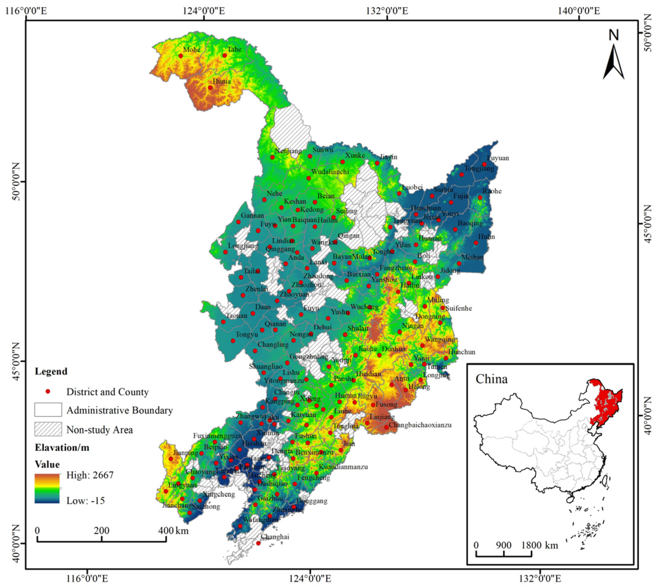
2.1. Object of Study

In this study, 142 counties in three provinces of Northeast China (Figure 1) were selected as research objects. The three provinces of Northeast China, Liaoning, Jilin and Heilongjiang provinces, are located in the northeast of China. They are one of the four major economic zones in China. They are important old industrial bases in China and have made great contributions to the construction of the whole country. In the early years of the founding of the People’s Republic of China, the three northeastern provinces focused on the development of heavy industry and resource-based industries by relying on their resources and geographical advantages and achieved a considerable increase in social and economic construction and population size. However, after the reform and opening up, the location advantage of the three provinces in northeast China gradually weakened, and China’s economic center of gravity began to shift to the southeast coastal areas. Under the common influence of the single heavy industrial structure, the increasingly depleted natural resources and the difficulties in the transformation and upgrading of industrial structure, a series of resource factors such as manpower, capital and technology have been outflowing in the three northeastern provinces [36]. Over the years, the economy of the three provinces in Northeast China has become relatively sluggish, with a series of problems such as the lagging development of the real economy, a low degree of economic marketization, the imperfect development of the market system, a low level of science and technology and low innovation ability. At the same time, in terms of population development, they are faced with the double pressure of population loss and population aging [31]. At present, the situation of population contraction in the three Northeast provinces directly poses a challenge to the coordinated and sustainable development and construction of regional society–economy–ecology. Therefore, this paper takes the three northeast provinces of China, which generally show problems such as slow economic development, population loss, urban decay and so on, as the research object.

2.2. Research Methods

2.2.1. Population Shrinkage Identification

According to different research perspectives, the methods of population shrinkage are different [37,38]. Based on reference to relevant literature, this paper uses the change rate of permanent population [8] to characterize the county population shrinkage index. The calculation formula is:

$$P_v=\frac{P_b-P_a}{P_a}\times 100\%$$

(1)

In the formula, P_v represents the change rate of permanent population. When P_v ≥ 0, it indicates that the population of the region is in a state of growth; when P_v < 0, it indicates that the population of the county is in a state of decline. P_a and P_b represent the total resident population in the base year and the end year of the study, respectively. The more the P_v value deviates from 0, the greater the degree of population reduction (increase). In this paper, the population change of 142 counties in the three provinces of Northeast China during the T1 (2000–2010) and T2 (2010–2020) periods was calculated by using the data of National “fifth, sixth and seventh” population statistics. (There were only three counties with severe contraction in the T1 period and one county with population growth in the T2 period. County units are too few and lack comparability and are not included in the comparative analysis of shrinking types below.) Counties with negative population change rates are defined as population shrinking counties.

2.2.2. Construction of the Indicator System

Referring to the relevant literature [39,40], combined with the actual situation of the county, adhering to the principles of scientificity, comparability and data availability, a county-level society–economy–ecology evaluation index system was constructed based on the three subsystems of society, economy and ecology, with 28 indicators selected (

Table 1. Evaluation index system of the comprehensive development level of the society–economy–ecology system in the county.

Normative Layer	Indicator Layer	Unit (of Measure)	Property	Weight
Social subsystem A	A1 Urbanisation rate	%	+	0.0964
	A2 Hospital beds per 10,000 persons	Couch	+	0.0761
	A3 Number of beds in various social welfare and adoption units per 10,000 persons	Couch	+	0.1002
	A4 Population density	Man /km2	+	0.1928
	A5 Average night-time light index	Lm/m2	+	0.2996
	A6 Housing floor space per capita	Man /m2	+	0.0706
	A7 Average years of schooling	Years	+	0.0834
	A8 Aging rate	%	−	0.0436
	A9 Illiteracy rate	%	−	0.0375
Economic subsystems B	B1 GDP per capita	Ten thousand yuan/man	+	0.1039
	B2 Gross regional product (GDP)	Ten thousand yuan	+	0.1631
	B3 Value added of secondary and tertiary industries as a share of GDP	%	+	0.0480
	B4 General local budget revenue per capita	Ten thousand yuan	+	0.1539
	B5 Local budget expenditure per capita	Ten thousand yuan	+	0.0996
	B6 Per capita urban and rural residents’ savings deposit balance	Ten thousand yuan	+	0.0874
	B7 Balance of loans from financial institutions at the end of the year per capita	Ten thousand yuan	+	0.1416
	B8 Number of industrial enterprises above designated size	General	+	0.2024
Ecological subsystem C	C1 Annual average PM2.5	Mg/m3	−	0.1288
	C2 Carbon dioxide emissions per capita	Hundred tonnes/man	−	0.0289
	C3 Degree of topographic relief		−	0.0482
	C4 Average Elevation	m	−	0.0466
	C5 Average annual wind speed	m/s	−	0.1096
	C6 Average slope	°	−	0.0620
	C7 Average annual precipitation	m	+	0.2237
	C8 Average annual temperature	°C	+	0.0796
	C9 Average annual relative humidity	% rh	+	0.0757
	C10 Normalised Difference Vegetation Index (NDVI)		+	0.0639
	C11 Air flow coefficient		+	0.1329

“+” for positive indicators, “−” for negative indicators.

). The social subsystem mainly selected nine indicators from four dimensions of living security capacity, basic construction level, resident population quality and prosperity degree. The use and density of lighting facilities can represent the overall prosperity level of an area. The larger the average nighttime light index value, the greater the light density and total intensity and the higher the development level of the area, reflecting the overall level of basic public service capacity and infrastructure construction. The economic subsystem selected eight indicators from the three dimensions of economic development level, government fiscal capacity and resident wealth; the ecological subsystem selected 11 indicators from the three dimensions of environmental quality, environmental comfort and ecological function. Among them, the air circulation coefficient, annual PM2.5 and per capita carbon dioxide emissions reflect environmental quality; the terrain roughness degree, average elevation, annual precipitation, annual temperature, annual relative humidity, annual wind speed and average slope reflect the ecological comfort degree. The Normalized Difference Vegetation Index (NDVI) can reflect the quantitative and relative abundance of the active radiation of green live vegetation and can be used to characterize vegetation physiological state, vegetation productivity and green biomass. Therefore, the Normalized Difference Vegetation Index (NDVI) was chosen to reflect ecological functions. The aging rate, illiteracy rate, terrain roughness, average elevation, annual average wind speed, average slope, annual average PM2.5 and per capita carbon dioxide emissions are negative indicators, while the rest are positive indicators.

2.2.3. Entropy Method

The concept of entropy comes from the field of thermodynamics; it is a physical quantity used to characterize the disorder of systems and is widely used in systems science. In this paper, the entropy method was used to determine the weight of each indicator. Before comparing each indicator, dimensionless processing was carried out on the original data in the indicator system. The calculation process is as follows:

$$\mathrm{Standardization} \mathrm{of} \mathrm{positive} \mathrm{indicators}: {x^{\prime }}_{ij}=\frac{x_{ij}-\min x_{ij}}{\max x_{ij}-\min x_{ij}}$$

(2)

$$\mathrm{Standardization} \mathrm{of} \mathrm{Negative} \mathrm{indicators}: {x^{\prime }}_{ij}=\frac{\max x_{ij}-x_{ij}}{\max x_{ij}-\min x_{ij}}$$

(3)

where x_ij is the original value of the j county of the i index and maxx_ij and minx_ij are the maximum and minimum values of the j county of the i index, respectively.

$$\mathrm{Calculate} \mathrm{the} \mathrm{proportion} \mathrm{of} \mathrm{the} \mathrm{j} \mathrm{county} \mathrm{region} \mathrm{in} \mathrm{the} \mathrm{i} \mathrm{index} {\mathrm{z}}_{\mathrm{ij}}: z_{ij}=\frac{{x^{\prime }}_{ij}}{{\displaystyle \sum _{i=1}^n{x^{\prime }}_{ij}}} \mathrm{j}=1, 2, \dots \mathrm{m}$$

(4)

$$\mathrm{Calculate} \mathrm{the} \mathrm{information} \mathrm{entropy} {\mathrm{v}}_{\mathrm{j}} \mathrm{of} \mathrm{each} \mathrm{index}: v_j=-k{\displaystyle \sum _{i=1}^n(p_{ij}\ln p_{ij}}), \mathrm{Where} \mathrm{k} \mathrm{is} \mathrm{a} \mathrm{constant} \mathrm{and} k=\frac{1}{\ln (n)}$$

(5)

Calculate the redundancy of information entropy f_i: f_i = 1 − vi

(6)

$$\mathrm{Calculate} \mathrm{the} \mathrm{weight} \mathrm{value} \mathrm{of} \mathrm{each} \mathrm{indicator} {\mathrm{w}}_{\mathrm{i}}: w_i=\frac{f_i}{{\displaystyle \sum _{i=1}^n{f}_i}} \mathrm{j}=1, 2, \dots \mathrm{m}$$

(7)

$$\begin{array}{l}\mathrm{Calculate} \mathrm{the} \mathrm{comprehensive} \mathrm{development} \mathrm{evaluation} \mathrm{value} \mathrm{of} \mathrm{each} \mathrm{system}: f(x)={\displaystyle \sum _{i=1}^n{a}_i{x^{\prime }}_{ij}}g(y)={\displaystyle \sum _{i=1}^n{b}_i{y^{\prime }}_{ij}}\\ h(z)={\displaystyle \sum _{i=1}^n{c}_i{z^{\prime }}_{ij}}\end{array}$$

(8)

In the formula, x′_ij, y′_ij and z′_ij are the standardized values of the social, economic and ecological systems in this paper after the elimination of dimensions; a_i, b_i and c_i are the weights of each index in the three subsystems of this study. The benefit functions of the three subsystems of society, economy and ecology are f(x), g(y) and h(z), respectively. In the following analysis, the benefit functions of the three subsystems are represented by U₁, U₂ and U₃, respectively.

2.2.4. Coupled Coordination Models

Coupling is a concept in physics that refers to the interaction and influence of the movement forms of two or more systems, which can represent the degree of mutual dependence and mutual restraint between systems. In this paper, the formula for the coupling coordination degree of the society–economy–ecology system was obtained through the coupling coordination model:

$$C={\left\{\frac{U1\times U2\times U3}{{\left[\left(U1+U2+U3\right)/3\right]}^3}\right\}}^{1/3}$$

(9)

T = αU₁ + βU₂ + δU₃

(10)

$$D=\sqrt{C\times T}$$

(11)

where C is the coupling degree, U₁, U₂ and U₃ are the comprehensive score of society, economy and ecology, respectively, and T is the comprehensive development evaluation value of the three systems; α, β and δ are the coefficients to be determined, and α + β + δ = 1. In this paper, we consider that society, economy and ecology are of equal importance, and thus we make α = β = δ = 1/3; D is the degree of coupling coordination.

2.2.5. Grey Correlation Model

The grey relational degree model measures the degree of correlation between things or system factors according to the similarity of the shape of sequence curves. This method is a combination of qualitative and quantitative methods and has the characteristics of simple calculation, wide applicability and low requirement for sample size [41]. The following is the calculation formula:

$$r_i=\frac{1}{n}\sum _{k=1}^n{\xi }_{i }(k)$$

(12)

where r_i indicates the grey correlation degree and n is the total number of counties. When 0 < r_i ≤ 0.35, it indicates that the correlation between the factors is weak; when 0.35 < r_i ≤ 0.65, it indicates that the correlation between the factors is medium; when 0.65 < r_i ≤ 0.85, it indicates that the correlation between the factors is strong; when 0.85 < r_i ≤ 1.00, it indicates that the correlation between the factors is extremely strong.

2.2.6. Bivariate Spatial Autocorrelation Models

Bivariate global spatial autocorrelation can be used to explore the spatial correlation between multiple variables, and this method can describe the correlation features of the spatial distribution of different elements [42]. Bivariate local spatial autocorrelation can express the spatial correlation and aggregation degree of the attribute value of a spatial unit and the same attribute value in its adjacent space. In this paper, bivariate global spatial autocorrelation and bivariate local spatial autocorrelation are used to conduct spatial empirical tests on the spatial differences and agglomeration trends of each subsystem level and coordination level in 142 counties in the three provinces of Northeast China. The calculation formula is as follows:

$${{\displaystyle I}}_{lm}^p={{\displaystyle z}}_l^p·{\displaystyle \sum _{q=1}^n{w}_{pq}·}{{\displaystyle z}}_m^q$$

(13)

in the formula: $I_{lm}^p$ is the bivariate (attributes l and m) global spatial autocorrelation index for the spatial unit p; w_pq denotes the spatial connection matrix between spatial units p, q; $z_l^p=\frac{X_l^p-{\overline{X}}_l}{{\sigma }_l}$;${ z}_m^q=\frac{X_m^q-{\overline{X}}_m}{{\sigma }_m}$; $X_l^p,X_m^q$ are the values of attributes l and m of spatialunits p and q, respectively;$\overline{X}$_l, $\overline{X}$_m denotes the average of the geographic attributes l and m; ${\sigma }_l{, \sigma }_m$ are the variances of geographic attributes l and m, respectively.

2.2.7. Obstacle Degree Model

With reference to relevant studies [22], this paper analyzes and diagnoses the influencing factors that hinder the coordinated development of society–economy–ecology coupling at county level in the three provinces of Northeast China. The calculation steps are as follows:

$$M_j=(1-X_j)\times (W_i\times P_{ij})\times 100\%/{\displaystyle \sum _{i=1}^{28}(1-}{X}_j)\times (W_i\times P_{ij}),B_i=M_{ij}$$

(14)

where M_j is the Obstacle degree of indicator j, B_i is the Obstacle degree of system i, X_ij is the standardised value of each indicator obtained using the extreme deviation standardization method, W_i is the weight of the ith system and P_ij is the weight of the jth indicator in the ith system.

2.3. Data Sources

This study focuses on 142 counties in three provinces of Northeast China as the research unit, covering the period from 2000 to 2020. The data used to determine population contraction were obtained from the fifth (2000), sixth (2010) and seventh (2020) national census data of the permanent population. The Average Night Lights Index was sourced from the Harvard Dataverse network platform for research (https://dataverse.harvard.edu/dataset.xhtml?persistentId=doi:10.7910/DVN/GIYGJU, accessed on 6 May 2023). Annual average PM2.5 data were provided by Columbia University’s Social Economic Data and Application Center, offering global annual PM2.5 concentration information (https://sedac.ciesin.columbia.edu/data/set/sdei-global-annual-gwr-pm2-5-modis-misr-seawifs-aod/data-download, accessed on 16 April 2023). DEM data were derived through calculations based on ASTER Global Digital Elevation Model V003 data. The Normalized Difference Vegetation Index (NDVI) was acquired from the GEE platform by downloading MOD13A3 products of MODIS satellite sensor data (https://developers.google.cn/earth-engine/, accessed on 20 April 2023). The air circulation coefficient originated from the European Meteorological Centre ERA-Interim database (http://apps.ecmwf.int/datasets/, accessed on 16 June 2023), while annual average wind speed data came from from China Meteorological Network Ground Climate Data Log Dataset (V3.0) (http://www.nmic.cn/, accessed on 18 June 2023). Other index data were derived from various sources such as the China County Statistical Yearbook, the provincial and municipal Statistical Yearbook and the National Economic and Social Development Statistical Bulletin of each city and county; any missing values were supplemented using interpolation methods or other approaches.

Identification and classification of population shrinkage.

Formula 1 was used to calculate the population change rates P1 and P2 of 142 counties during T1 and T2 (Figure 2), and according to their change rates, the population shrinkage degree was divided into four categories: population growth type, mild contraction type, moderate contraction type and severe contraction type (

Table 2. County distribution of population contraction types in two periods based on the resident population index.

Phase	Type	Interval	Number of Counties	Proportions%	Phase	Type	Interval	Number of Counties	Proportions%
T1	Population growth	≥0%	61	42.96%	T2	Population growth	≥0%	1	0.70%
	Mild Population contraction	(0.0%, −10%]	67	47.18%		Mild Population contraction	(0.0%, −10%]	14	9.86%
	Moderate Population contraction	(−10%, −20%]	11	7.75%		Moderate Population contraction	(−10%, −20%]	45	31.69%
	Severe Population contraction	≤−20%	3	2.11%		Severe Population contraction	≤−20%	82	57.75%

). In T1, 81 counties showed a trend of population contraction, and the number of counties with population contraction reached 57.04%, but there were still 61 counties with population growth, showing a mixed situation in general. In the T2 period, the population showed an accelerated contraction trend, and the number of counties with population contraction increased to 141, accounting for 99.3%, while the number of counties with population growth was only 1. The region had entered a state of comprehensive contraction, and the contraction amplitude increased significantly.

3. Analysis of the Spatial-Temporal Correlation between Population Shrinkage and Social, Economic, Ecological and Synthetical Development Levels

In order to explore the spatiotemporal correlation between population shrinkage and social, economic, ecological and synthetical development level, the grey correlation degree and bivariate spatial autocorrelation analysis were used to calculate the population shrinkage index in T1 and T2 and the development level values in the last years of population change (2010 and 2020) to reveal the spatiotemporal relationship between them. The mean value of the horizontal value was used to express the result, and the Arcgis10.7 software was used for spatial visualization processing (Figure 3).

3.1. The Correlation between Population Shrinkage and Development Level

As can be seen from

Table 3. Grey correlation degree between population contraction index and social, economic, ecological and synthetical development level.

T1	Level of Development	Society	Economy	Ecology	Synthesis
	Gray correlation (r)	0.682	0.657	0.605	0.581
T2	Level of development	Society	Economy	Ecology	Synthesis
	Gray correlation (r)	0.756	0.604	0.646	0.692
Average value	Level of development	Society	Economy	Ecology	Synthesis
	Gray correlation (r)	0.719	0.631	0.626	0.637

, during the T1 period, the county population shrinkage index showed a strong correlation with social and economic development level, and the gray correlation degree was greater than 0.65, among which the correlation degree between the population shrinkage index and social development level was the highest, reaching 0.682. The correlation between the population shrinkage index and ecological and synthetical development level was medium, and the correlation between the population shrinkage index and synthetical development level was the lowest, 0.581. In T2, the county population shrinkage index showed a strong correlation with the level of social and synthetical development, and the grey correlation degree reached 0.756 and 0.692, respectively. The correlation between the population shrinkage index and economic and ecological development level was medium, and the correlation between the population shrinkage index and economic development level was 0.604. From the perspective of the average grey correlation degree between the population shrinkage index and the four development levels in the two periods, the evolution of society (0.719) > synthesis (0.637) > economy (0.631) > ecology (0.626) shows that population shrinkage has a strong correlation with social development level but a weak relationship with ecological development level.

3.2. Time Variation Characteristics of the Relationship between Population Contraction and Development Level

According to

Table 4. Social, economic, ecological and synthetical average development level of counties with different population contraction types (Due to the fact that there are only 3 counties with severe contraction in T1 period and 1 county with population growth in T2 period, there are too few county units and lack of comparability, so they are not included in the following comparative analysis of contraction types, and gray color has been used for marking).

T1 (Society)						T2 (Society)
County Type	2000	2010	Difference	Average Value	Growth Rate	County Type	2010	2020	Difference	Average Value	Growth Rate
Population growth	0.2332	0.2544	0.0212	0.2438	9.09%	Population growth	0.5711	0.5357	−0.0354	0.5534	−6.20%
Mild Population contraction	0.2143	0.2286	0.0143	0.2214	6.69%	Mild Population contraction	0.2762	0.2829	0.0067	0.2795	2.43%
Moderate Population contraction	0.2149	0.2095	−0.0054	0.2122	−2.51%	Moderate Population contraction	0.2611	0.2625	0.0014	0.2618	0.53%
Severe Population contraction	0.2587	0.3166	0.0579	0.2876	22.38%	Severe Population contraction	0.2183	0.2207	0.0024	0.2195	1.10%
Average value	0.2302	0.2523	0.0220	0.2413	9.56%	Average value	0.3317	0.3254	−0.0062	0.3286	−1.88%
Extreme deviation	0.0444	0.1071	0.0627	0.0757	141.15%	Extreme deviation	0.3528	0.3150	−0.0378	0.3339	−10.72%
T1 (Economy)						T2 (Economy)
County Type	2000	2010	Difference	Average value	Growth rate	County Type	2010	2020	Difference	Average value	Growth rate
Population growth	0.2012	0.1867	−0.0145	0.1940	−7.21%	Population growth	0.3438	0.2740	−0.0698	0.3089	−20.30%
Mild Population contraction	0.1725	0.1848	0.0123	0.1787	7.15%	Mild Population contraction	0.2607	0.1949	−0.0658	0.2278	−25.23%
Moderate Population contraction	0.1622	0.1644	0.0023	0.1633	1.41%	Moderate Population contraction	0.2322	0.1760	−0.0563	0.2041	−24.23%
Severe Population contraction	0.2635	0.2553	−0.0082	0.2594	−3.09%	Severe Population contraction	0.1452	0.1504	0.0052	0.1478	3.58%
Average value	0.1998	0.1978	−0.0020	0.1988	−1.00%	Average value	0.2455	0.1988	−0.0467	0.2221	−19.01%
Extreme deviation	0.1013	0.0909	−0.0104	0.0961	−10.31%	Extreme deviation	0.1986	0.1237	−0.0750	0.1612	−37.75%
T1 (Ecology)						T2 (Ecology)
County Type	2000	2010	Difference	Average value	Growth rate	County Type	2010	2020	Difference	Average value	Growth rate
Population growth	0.5222	0.4863	−0.0359	0.5043	−6.87%	Population growth	0.4751	0.4887	0.0136	0.4819	2.86%
Mild Population contraction	0.5225	0.4925	−0.0300	0.5075	−5.74%	Mild Population contraction	0.4826	0.4722	−0.0104	0.4774	−2.15%
Moderate Population contraction	0.5276	0.5029	−0.0247	0.5153	−4.67%	Moderate Population contraction	0.5061	0.4885	−0.0175	0.4973	−3.46%
Severe Population contraction	0.6163	0.5783	−0.0380	0.5973	−6.17%	Severe Population contraction	0.4869	0.4802	−0.0067	0.4836	−1.37%
Average value	0.5471	0.5150	−0.0321	0.5311	−5.87%	Average value	0.4877	0.4824	−0.0052	0.4850	−1.07%
Extreme deviation	0.0941	0.0919	−0.0022	0.0930	−2.30%	Extreme deviation	0.0309	0.0165	−0.0144	0.0237	−46.49%
T1 (Synthesis)						T2 (Synthesis)
County Type	2000	2010	Difference	Average value	Growth rate	County Type	2010	2020	Difference	Average value	Growth rate
Population growth	0.2684	0.2598	−0.0086	0.2641	−3.21%	Population growth	0.4409	0.4091	−0.0318	0.4250	−7.22%
Mild Population contraction	0.2485	0.2514	0.0029	0.2499	1.15%	Mild Population contraction	0.3034	0.2779	−0.0255	0.2906	−8.39%
Moderate Population contraction	0.2452	0.2366	−0.0085	0.2409	−3.48%	Moderate Population contraction	0.2881	0.2649	−0.0232	0.2765	−8.06%
Severe Population contraction	0.3213	0.3302	0.0089	0.3258	2.77%	Severe Population contraction	0.2272	0.2365	0.0094	0.2318	4.13%
Average value	0.2708	0.2695	−0.0013	0.2702	−0.50%	Average value	0.3149	0.2971	−0.0178	0.3060	−5.65%
Extreme deviation	0.0761	0.0936	0.0174	0.0849	22.90%	Extreme deviation	0.2138	0.1726	−0.0412	0.1932	−19.27%

, the development levels of social, economic, ecological and synthetical systems in counties with different types of population shrinkage during T1 and T2 were compared and summarized to reveal the correlation characteristics between population shrinkage and regional development levels. On the whole, the development level of the three subsystems and the synthetical system in the counties of different population contraction types during the T1 period showed the relationship from high to low as ecological > synthetical > social > economic system. The development level of the social and economic system was relatively low, all of which were less than 0.25, and the economic development level was the lowest, only 0.1988, indicating that the economic development level was relatively lagging behind. The level of ecological development was higher, reaching 0.5311. From the perspective of development speed, in addition to the positive growth rate of the social development level, the growth rate of economic, ecological and synthetical level was negative, indicating that the level of social development was improved at this stage, but the level of economic, ecological and synthetical development showed a downward trend, and the economy and society showed a serious development dislocation phenomenon and were in a period of economic and social development run-in disorder. From the perspective of the difference in development level between the three sub-systems, the social system had the highest growth rate (141.15%), showing a large divergence trend. The economic system had the lowest-range growth rate (−10.31%), which shows an obvious convergence trend, which indicates that the inequality of social development among counties of different contraction types increased significantly while the imbalance of economic development decreased. The inequality in the development level of the synthetical system increased, and the development level of the ecological system was relatively stable. Comparing the development level of counties with different subsystems and different types of population shrinkage showed a significant shrinkage effect, and the social, economic and synthetical development level of counties with different types of population shrinkage showed the following. The evolution characteristics of population growth type > mild contraction type > moderate contraction type show that the degree of population contraction in a county is negatively correlated with the level of social, economic and synthetical development, and the higher the degree of population contraction, the lower the level of development, which indicates that population contraction comprehensively reflects the effect and feedback effect of low social and economic level. The level of ecological development in counties with different types of population shrinkage showed the following evolutionary characteristics: moderate contraction type > mild contraction type > population growth type. The degree of population shrinkage in counties showed a significant positive correlation with the level of ecological development, and the greater the degree of population shrinkage, the higher the level of development, which may be related to the reduction in regional ecological environment pressure caused by population shrinkage. In the T2 period, the relationship between the development level of the three subsystems and the synthetical system was relatively stable, which is shown as ecology > society > synthesis > economy. The growth rate of the development level of the four types of systems was negative and showed a downward trend. From the perspective of development speed, the growth rate of social development level in counties of different population contraction types was positive, while the ecological development level was negative, while the growth rate of the economic and synthetical development level did not show regular changes. From the perspective of the difference in development level in different contracting types of the three subsystems, the growth rate of the ecological system range was the lowest (−46.49%), indicating that the imbalance in the county ecological system showed an obvious convergence trend at this stage. The development level of counties with different subsystems and population shrinkage types showed a significant contraction effect. The evolution characteristics of the social, economic and synthetical development level of counties with different population shrinkage types were: mild contraction type > moderate contraction type > severe contraction type. The degree of population shrinkage of counties was significantly negatively correlated with social, economic and synthetical development level. The average level of ecological development in counties with different population shrinking types did not show significant regularity, and the correlation between the two was not significant.

3.3. Spatial Pattern Characteristics of Population Contraction and Development Level

3.3.1. Global Autocorrelation

It can be seen from

Table 5. Bivariate Moran’s I of population contraction and social, economic, ecological and synthetical development levels.

Spatial Correlation	T1	T2
Population contraction and level of social development	−0.0656 *	0.1287 **
Population contraction and level of economic development	−0.1275 **	0.1463 **
Population contraction and level of ecological development	−0.0685 *	−0.028
Population contraction and level of synthetical development	−0.123 **	0.1486 **

Note: * indicates passing the 5% significance test; ** indicates passing the 1% significance test.

that Moran’s I between the population contraction index in T1 period and the four development levels are all negative, with significant spatial heterogeneity. The Moran’s I between the population contraction index and the social, economic and synthetical development level in the T2 period is positive, indicating that the population contraction index shows a significant spatial positive correlation with the three types of development levels, that the interaction between the development levels of counties is strong and that the counties with a high development level tend to be adjacent in space while those with a low development level also tend to be adjacent in space. The Moran’s I value of the bivariate of population contraction index and ecological development level is negative and fails the significance test, indicating that the temporal and spatial correlation between population contraction and ecological development level in the T2 stage is relatively weak.

3.3.2. Local Autocorrelation

As can be seen from Figure 3, the population increased or slightly shrank during T1, and the high-high-concentration areas in counties that had high levels of social, economic, ecological and synthetical development are mainly distributed in the southern region with the central and southern Liaoning city clusters as the core. The low-low cluster with a high population shrinkage index and a low ecological development level was dispersed, and the spatial fragmentation pattern was obvious, distributed in western Liaoning, the Greater Khingan Mountains, the Changbai Mountains and northern parts. The low-low clusters with large population shrinkage and a low level of social, economic and synthetical development are distributed in the central and western regions and the northern regions. The population growth was slow, and the population contraction was serious. The low-high agglomeration areas with relatively high social, economic, ecological and synthetical development levels are mainly distributed in the southern high-high agglomeration area. The population growth or population contraction trend was relatively slow, and the social, economic, ecological and synthetical development level is relatively low in the high-low agglomeration area mainly distributed in the west and the north-central low-low agglomeration area. Similar to the T1 period, the high-high agglomeration was still mainly distributed in the southern part of the region in the T2 period, and the low-low agglomeration was still distributed in the central and eastern parts of the region and the northwest part of the region. Compared with T1, the amount of low-high agglomeration and high-low agglomeration decreased significantly, among which the low-high agglomeration was still distributed in the surrounding areas of high-high agglomeration, and the high-low agglomeration area was still mainly distributed around the low-low agglomeration area. On the whole, the southern and eastern regions of the three northeastern provinces had a relatively high level of overall development and relatively moderate population contraction due to a relatively developed society and economy and a good ecological environment, while the central and northwestern regions had a relatively low overall development level and relatively severe population contraction due to a relatively backward society and economy and a relatively poor ecological environment.

4. Analysis of the Spatial and Temporal Correlation between Population Contraction and Coordinated Social, Economic and Ecological Development

In order to further explore the correlation between population contraction and the coordinated development of the society–economy–ecology system in the three provinces of Northeast China, the pair-and-pair coupling of population contraction with the three subsystems and the coordinated development level of the three subsystems were analyzed. Formulas (12) and (13) were used to calculate the population contraction index of T1 and T2 and the society–economy–ecology coupling and the coordination level of the three coupling levels at the end of the period. The grey correlation degree and bivariate spatial autocorrelation analysis were carried out to reveal the spatiotemporal correlation characteristics of the two, and spatial visualization processing was conducted by Arcgis10.7 software (Figure 4).

4.1. The Level Correlation between Population Shrinkage and Coordination Degree

As can be seen from

Table 6. Grey correlation degree between the population contraction index and the level of society–economy–ecology coordinated development.

T1	Coordination Degree Development Level	Society -Economy	Society-Ecology	Economy-Ecology	Society-Economy-Ecology
	Gray correlation (r)	0.64	0.525	0.587	0.619
T2	Coordination degree development level	Society -Economy	Society-Ecology	Economy-Ecology	Society-Economy-Ecology
	Gray correlation (r)	0.784	0.776	0.732	0.764
Average value	Coordination degree development level	Society -Economy	Society-Ecology	Economy-Ecology	Society-Economy-Ecology
	Gray correlation (r)	0.712	0.651	0.660	0.692

, during the T1 period, the correlation degree between the population shrinkage index and the coupling coordination degree level of the four types of systems in the three provinces of Northeast China was moderate. Among them, the correlation degree between the population shrinkage index and the coordination degree level of the society–economy system was 0.64 at the highest, and the correlation degree between the population shrinkage index and the coordination degree level of the society–ecology system was 0.525 at the lowest. In the T2 period, the population shrinkage index showed a strong correlation with the level of the coupling coordination degree of the four types of systems, and the grey correlation degree was greater than 0.65, among which the correlation degree between the population shrinkage index and the coordination degree of the society–economy system was the highest, reaching 0.784. The correlation between population contraction index and the economy–ecology system was the lowest at 0.732. In general, the average grey correlation degree between the population contraction index and the four coordination degree levels during the study period showed an evolutionary trajectory of society–economy (0.712) > society–economy–ecology (0.692) > economy–ecology (0.660) > society–ecology (0.651), and the correlation degree between population contraction and the development level of society–ecology coordination degree was relatively weak.

4.2. Time Variation Characteristics of the Horizontal Correlation between Population Shrinkage and Coordination Degree

As can be seen from

Table 7. Development level of society–economy–ecology average coordination degree in counties with different population shrinking types (Due to the fact that there are only 3 counties with severe contraction in T1 period and 1 county with population growth in T2 period, there are too few county units and lack of comparability, so they are not included in the following comparative analysis of contraction types, and gray color has been used for marking).

T1 (Society-Economy)						T2 (Society-Economy)
County Type	2000	2010	Difference	Average Value	Growth Rate	County Type	2010	2020	Difference	Average Value	Growth Rate
Population growth	0.4519	0.4448	−0.0071	0.4483	−1.57%	Population growth	0.6657	0.6190	−0.0467	0.6423	−7.01%
Mild Population contraction	0.4311	0.4429	0.0118	0.4370	2.73%	Mild Population contraction	0.5035	0.4757	−0.0278	0.4896	−5.52%
Moderate Population contraction	0.4272	0.4251	−0.0021	0.4262	−0.50%	Moderate Population contraction	0.4793	0.4521	−0.0272	0.4657	−5.68%
Severe Population contraction	0.5051	0.5169	0.0118	0.5110	2.34%	Severe Population contraction	0.4116	0.4196	0.0081	0.4156	1.96%
Average value	0.4538	0.4574	0.0036	0.4556	0.79%	Average value	0.5150	0.4916	−0.0234	0.5033	−4.55%
Extreme deviation	0.0779	0.0918	0.0139	0.0848	17.91%	Extreme deviation	0.2541	0.1994	−0.0548	0.2267	−21.55%
T1 (Society-Ecology)						T2 (Society-Ecology)
County Type	2000	2010	Difference	Average value	Growth rate	County Type	2010	2020	Difference	Average value	Growth rate
Population growth	0.5831	0.5863	0.0032	0.5847	0.54%	Population growth	0.7218	0.7153	−0.0064	0.7185	−0.89%
Mild Population contraction	0.5751	0.5770	0.0019	0.5761	0.33%	Mild Population contraction	0.6011	0.6018	0.0007	0.6015	0.12%
Moderate Population contraction	0.5785	0.5683	−0.0102	0.5734	−1.76%	Moderate Population contraction	0.5958	0.5900	−0.0058	0.5929	−0.98%
Severe Population contraction	0.6277	0.6415	0.0138	0.6346	2.20%	Severe Population contraction	0.5689	0.5677	−0.0012	0.5683	−0.20%
Average value	0.5911	0.5933	0.0022	0.5922	0.37%	Average value	0.6219	0.6187	−0.0032	0.6203	−0.51%
Extreme deviation	0.0526	0.0732	0.0207	0.0629	39.33%	Extreme deviation	0.1528	0.1476	−0.0053	0.1502	−3.45%
T1 (Economy-Ecology)						T2 (Economy-Ecology)
County Type	2000	2010	Difference	Average value	Growth rate	County Type	2010	2020	Difference	Average value	Growth rate
Population growth	0.5555	0.5240	−0.0315	0.5397	−5.66%	Population growth	0.6357	0.6049	−0.0308	0.6203	−4.84%
Mild Population contraction	0.5403	0.5368	−0.0034	0.5386	−0.63%	Mild Population contraction	0.5805	0.5411	−0.0394	0.5608	−6.79%
Moderate Population contraction	0.5361	0.5287	−0.0074	0.5324	−1.38%	Moderate Population contraction	0.5686	0.5321	−0.0365	0.5503	−6.41%
Severe Population contraction	0.6294	0.6116	−0.0178	0.6205	−2.83%	Severe Population contraction	0.5028	0.5107	0.0079	0.5068	1.56%
Average value	0.5653	0.5503	−0.0150	0.5578	−2.66%	Average value	0.5719	0.5472	−0.0247	0.5596	−4.32%
Extreme deviation	0.0933	0.0876	−0.0057	0.0905	−6.15%	Extreme deviation	0.1329	0.0942	−0.0387	0.1136	−29.09%
T1 (Society-Economy-Ecology)						T2 (Society-Economy-Ecology)
County Type	2000	2010	Difference	Average value	Growth rate	County Type	2010	2020	Difference	Average value	Growth rate
Population growth	0.5260	0.5134	−0.0126	0.5197	−2.40%	Population growth	0.6735	0.6446	−0.0288	0.6590	−4.28%
Mild Population contraction	0.5111	0.5149	0.0039	0.5130	0.76%	Mild Population contraction	0.5591	0.5366	−0.0225	0.5479	−4.03%
Moderate Population contraction	0.5094	0.5031	−0.0062	0.5062	−1.23%	Moderate Population contraction	0.5444	0.5208	−0.0235	0.5326	−4.32%
Severe Population contraction	0.5842	0.5866	0.0023	0.5854	0.40%	Severe Population contraction	0.4892	0.4950	0.0058	0.4921	1.18%
Average value	0.5327	0.5295	−0.0032	0.5311	−0.60%	Average value	0.5665	0.5493	−0.0173	0.5579	−3.05%
Extreme deviation	0.0749	0.0834	0.0086	0.0791	11.47%	Extreme deviation	0.1843	0.1496	−0.0346	0.1670	−18.80%

, from the coordination level of different coupled systems, the coordination degree level in the T1 period showed the sequence of society–ecology > economy–ecology > society–economy–ecology > society–economy system from high to low, in which the level of society–economy coordination is low, with an average value of 0.4556. It further shows that the level of coordination between the two was low due to the dislocation of social and economic development. From the perspective of development speed, the growth rate of economy–ecology and society–economy–ecology system coordination degree was negative, and the coordination level was decreased, while the society–economy and society–ecology system basically maintained their original level. From the perspective of difference in development level, the highest growth rate (39.33%) was found among counties with different types of population shrinkage, showing a significant divergence trend. The economy–ecology system showed the lowest growth rate (−6.15%) and showed convergence. Society–economy and society–economy–ecology system disparities were increasing. Comparing counties with different coupling systems and different population shrinking types, it is found that the population shrinking counties all showed significant shrinking effects. Specifically, society–economy–ecology coupling and triplex coupling coordinated development levels of counties with different population shrinking types show: The evolution characteristics of population growth type > mild contraction type > moderate contraction type showed that the degree of population contraction was negatively correlated with the development level of coordination degree. The higher the degree of population contraction, the lower the development level of coordination degree. The coordination degree level of different coupling systems in the T2 period showed the sequence of society–ecology > economy–ecology > society–economy–ecology > society–economy system from high to low, and the coordination degree level of the society–economy system was still the lowest, and the run-in interaction between social and economic development was still not good. From the perspective of development speed, the growth rate of the coordinated development level of the four different coupling systems was negative, and the coordination degree level showed a downward trend. From the perspective of the difference in the coordination level of different coupling systems between counties with different population shrinkage types, the growth rate of the economy–ecology range was the lowest of −29.09%, showing a significant convergence trend. After comprehensive comparison, it is found that the population shrinking county showed a significant shrinking effect. Different population shrinkage types and the coordinated development levels of the four different coupling systems showed the evolution characteristics of mild contraction type > moderate contraction type > severe contraction type, and the population shrinkage and coordination degree were negatively correlated. The population growth county had a factor agglomeration effect on the surrounding areas in the aspects of society and economy, strong ecological protection and construction ability and a high coordination level. The social and economic development level of counties with mild shrinkage was lower than that of counties with population growth, because the outflow of development factors caused by population shrinkage has a negative impact on social and economic development and ecological construction capacity. Due to the weak development foundation and the gradually increasing negative effect of population contraction, the development factors accelerated the outflow of the county, which further hindered the upgrading of the county’s industrial structure and improvement in the overall social development level, weakened the county’s ecological governance ability and hindered improvement in the coordination level. Counties with severe contraction were faced with the double negative effects of population contraction and a serious loss of development factors, the social and economic development lagged behind, and the mismatch with the ecological development level led to a low coordination level.

4.3. Spatial Pattern Characteristics of Population Shrinkage and Coordination Degree

4.3.1. Global Autocorrelation

It can be seen from

Table 8. Bivariate Moran’s I of society–economy–ecology coordination.

Spatial Correlation	T1	T2
Population contraction and level of society-economy coordination	−0.1259 **	0.1653 **
Population contraction and level of society-ecology coordination	−0.0802 **	0.1118 **
Population contraction and level of economy-ecology coordination	−0.139 **	0.1475 **
Population contraction and level of society-economy-ecology coordination	−0.1297 **	0.157 **

Note^: ** indicates passing the 1% significance test.

that the Moran’s I of population contraction index in the T1 period and the coordination degree of society–economy, society–ecology, economy–ecology and society–economy–ecology system were all negative, and there was significant spatial heterogeneity between the two. The Moran’s I values of the population contraction index and the coordination degree levels of the society–economy, society–ecology, economy–ecology and society–economy-ecology system in the T2 stage were all positive, indicating that the population contraction index was significantly positively correlated with the coordination degree of the four systems. The interaction of the development level of coordination degree among counties was strong, indicating that the counties with a high coordination degree tended to be adjacent in space and the counties with a low coordination degree tended to be adjacent in space.

4.3.2. Local Autocorrelation

After processing with the Geoda and arcgis10.7 software, LISA cluster plots of population shrinkage and coordination degree levels of four coupled systems of society–economy, society–ecology, economy–ecology and society–economy–ecology in the three provinces of Northeast China were obtained (Figure 4). As can be seen from Figure 4, the bivariate local spatial autocorrelation spatial distribution pattern of the coordination degree level between population contraction and the four coupled systems in the T1 period is similar to the development level of population contraction and the three subsystems and the synthetical system mentioned above. High-high agglomeration is mainly distributed in the south, low-low agglomeration is concentrated in the central and northwestern regions, low-high agglomeration is mainly distributed in the southern regions around high-high agglomeration, and high-low agglomeration is mainly distributed in the western and north-central regions around low-low agglomeration. Similar to the T1 period, the high-high concentration in T2 period was still mainly distributed in the south, with sporadic distribution in the east. Low-low concentration is still distributed in the eastern and northwestern parts. The number of low-high agglomeration and high-low agglomeration decreased significantly, and low-high agglomeration was mainly distributed in the south and east. High-low agglomeration was still mainly distributed around the low-low agglomeration.

5. Analysis of the Correlation between Population Contraction and Obstacles to Coordinated Development

In order to explore the effects of population contraction and the coordinated development of the system, this paper identifies and analyzes the main obstacle factors that affect the coordinated development of the system under different types of population contraction and measures the obstacle degrees of three subsystems and their single indicators in the T1 and T2 periods (

Table 9. Factors analysis of social–economic–ecological coupling coordination obstacles in the T1 and T2 periods.

T1time Period (Population Growth)				T1time Period (Mild Population Contraction)				T1time Period (Moderate Population Contraction)
Obstacle Degree (%)	2000	2010	Average Value	Obstacle Degree (%)	2000	2010	Average Value	Obstacle Degree (%)	2000	2010	Average Value
Social subsystem (A)	43.74%	33.78%	38.76%	Social subsystem (A)	39.43%	35.18%	37.31%	Social subsystem (A)	39.55%	34.62%	37.08%
Economic subsystems (B)	46.35%	55.28%	50.82%	Economic subsystems (B)	43.03%	47.58%	45.31%	Economic subsystems (B)	34.41%	42.84%	38.62%
Ecological subsystem (C)	9.91%	10.94%	10.43%	Ecological subsystem (C)	17.54%	17.24%	17.39%	Ecological subsystem (C)	26.04%	22.54%	24.29%
B8	8.60%	18.12%	13.36%	A5	13.63%	8.39%	11.01%	B8	3.60%	11.06%	7.33%
A5	14.96%	9.54%	12.25%	B2	9.32%	7.38%	8.35%	A5	8.17%	5.87%	7.02%
B2	8.88%	8.18%	8.53%	B8	5.67%	10.58%	8.13%	B5	5.95%	7.38%	6.66%
B6	7.09%	8.33%	7.71%	B7	3.81%	10.41%	7.11%	B2	3.95%	8.18%	6.07%
B4	6.42%	7.88%	7.15%	B4	6.39%	6.64%	6.51%	A1	4.61%	7.08%	5.85%
A4	6.76%	6.89%	6.83%	B5	6.23%	5.62%	5.92%	B4	6.90%	3.52%	5.21%
B5	6.63%	3.52%	5.08%	A4	5.54%	5.45%	5.49%	B6	3.72%	6.26%	4.99%
A2	6.38%	2.41%	4.40%	A2	3.53%	5.91%	4.72%	A4	4.41%	4.78%	4.59%
A3	3.53%	4.20%	3.86%	A1	4.50%	4.06%	4.28%	A3	5.31%	3.68%	4.49%
B7	3.04%	4.64%	3.84%	B1	4.46%	3.87%	4.17%	C1	4.21%	4.19%	4.20%
T2time period (Mild population contraction)				T2time period (Moderate population contraction)				T2time period (Severe Population contraction)
Obstacle degree (%)	2010	2020	average value	Obstacle degree (%)	2010	2020	average value	Obstacle degree (%)	2010	2020	average value
Social subsystem (A)	33.17%	28.07%	30.62%	Social subsystem (A)	34.08%	35.72%	34.90%	Social subsystem (A)	35.16%	34.29%	34.72%
Economic subsystems (B)	39.24%	47.35%	43.30%	Economic subsystems (B)	51.96%	44.41%	48.18%	Economic subsystems (B)	49.32%	53.13%	51.22%
Ecological subsystem (C)	27.59%	24.58%	26.09%	Ecological subsystem (C)	13.96%	19.88%	16.92%	Ecological subsystem (C)	15.52%	12.58%	14.05%
B2	9.10%	9.70%	9.40%	A5	10.50%	13.09%	11.79%	A5	9.73%	13.52%	11.63%
B8	8.71%	4.79%	6.75%	B8	12.68%	8.56%	10.62%	B7	4.01%	16.01%	10.01%
B7	3.25%	9.57%	6.41%	A4	9.00%	9.04%	9.02%	B8	12.64%	5.94%	9.29%
B4	6.41%	5.27%	5.84%	B7	9.99%	6.73%	8.36%	B4	8.93%	8.89%	8.91%
B1	4.83%	5.93%	5.38%	B2	8.49%	6.26%	7.38%	B1	5.02%	9.16%	7.09%
A3	5.73%	4.66%	5.20%	B4	6.80%	7.51%	7.16%	B2	7.85%	4.67%	6.26%
B5	2.69%	6.88%	4.79%	B5	5.62%	5.75%	5.69%	A4	5.17%	5.31%	5.24%
A1	4.74%	4.57%	4.66%	C7	3.75%	6.43%	5.09%	B6	4.97%	3.81%	4.39%
C7	4.45%	4.53%	4.49%	B1	3.57%	5.20%	4.38%	A7	4.67%	3.95%	4.31%
A2	4.98%	3.78%	4.38%	B6	3.93%	2.78%	3.36%	A1	5.18%	3.11%	4.14%

Note: Due to space constraints of the article, obstacle indicators are represented by codes.

). Due to the large number of single indicators, this paper only analyzes the top 10 factors in the order of obstacle degrees. The factors ranked 1–5 are defined as important obstacle factors, and the factors ranked 5–10 are defined as major obstacle factors.

5.1. Analysis of the Correlation between Population Contraction and the Obstacles to Coordinated Development Degree Factor, 2000–2010

As can be seen from Table 9, the obstacle degree of the three subsystems to the overall coordinated development in the T1 period is quite different, and the obstacle degree of the criterion layer and indicator layer of counties with different population contraction types is different, showing the phenomenon of economic subsystem > social subsystem > ecological subsystem on the whole. In terms of index layer, the top 10 obstacle factors of population growth counties were all social and economic system indicators, accounting for 73.00% of the total obstacle degree. The top 10 obstacle factors in the mild shrinkage county index were all social and economic system indicators, accounting for 65.70% of the total obstacle degree. The obstacle degree of the top 10 index layers in moderate shrinkage county accounted for 56.42% of the whole, of which there were nine indicators of the social and economic subsystem and only one indicator of ecological system. In general, the proportion of the top 10 obstacle factors in the index layer of different population contraction types in T1 showed a gradient change pattern of population growth > mild contraction > moderate contraction, indicating that the lower the degree of population contraction, the stronger the effect of the top 10 obstacle factors and the dominant factors. With an increase in population shrinkage, the non-dominant factors are relatively enhanced, the obstacle factors tend to disperse, and the obstacle factors of the three subsystems tend to be balanced. The common important obstacle factors of the three types of population shrinking counties are the number of industrial enterprises above designated size, average night light index and gross regional product, and the common main obstacle factor is population density. Society and economy are the core obstacle factors restricting coordinated development. Vigorously developing the economy and improving the level of social development are the important direction of efforts to reduce the factor obstacle degree, as well as the key to improve the level of coordinated development of the system. The level of social and economic development is the important basis of regional population carrying capacity, as well as the core driving force of the coordinated development of social, economic and ecological. Among the common obstacles, the number of industrial enterprises above designated size plays a strong restricting role. Developing the industrial economy according to local conditions and improving the quantity and quality of industrial enterprises are common development problems faced by county economic development. All counties should focus on cultivating and guiding high-quality enterprises, improving the scale and quality of employment positions, optimizing industrial structures and promoting the coordinated development of social and economic subsystems. The average night light index implies the quality of basic public service supply and the level of infrastructure construction, and it is an important embodiment of a regional social development level. Supporting emerging industries, implementing innovative development and comprehensively improving the level of economic development are important supports to reduce the obstacle degree. Alleviating the pressure of population contraction, improving the quality of population in an all-round way and managing the problem of population development are the key points to break the hindrance of social subsystem factors of different types of population contraction.

5.2. Analysis of the Correlation between Population Contraction and the Obstacles to Coordinated Development Degree Factor, 2010–2020

It can be seen from Table 9 that the obstacle degree of criterion layer and indicator layer of counties with different population contraction types in the T2 period is different, but the overall pattern is economic subsystem > social subsystem > ecological subsystem. The top 10 obstacle factors in the index layer of mild contracted counties accounted for 57.30% of the total obstacle degree with a proportion of 38.46%, and the economic, social and ecological system indexes were 6, 3 and 1, respectively. The obstacle degree of index layer in moderate shrinkage county accounted for 72.84%, nine social and economic indexes and one ecological index. The obstacle degree of the top 10 index layers in the county with severe contraction accounted for 71.28% of the whole, all of which were indicators of the social and economic subsystem. In general, the obstacle degree of the social subsystem, the economic subsystem and the ecological subsystem showed a trend of decline among counties with different population contraction types in the T2 period. The common important obstacle factors of the three types of population contraction counties are the number of industrial enterprises above designated size and the per capita balance of loans from financial institutions at the end of the year. Economic factors were still the core obstacle to the coordinated development of the three provinces in Northeast China. The per capita loan balance of financial institutions at the end of the year was closely related to the level of regional financial development, and the level of financial development was related to local economic construction. Improving financial supply to promote economic growth is the focus of cracking the obstacle factors. To sum up, during the study period, in the process of the coordinated development of society, economy and ecology in the three Northeast provinces, the obstacle degree of economic and social subsystems has always been in the dominant position, which is the main obstacle factor affecting the coordinated development. The reasons are as follows: The lagging level of social and economic development and the stagnation and decline of economic development result in the low level of coordination in the social and economic subsystems, and the realization of population growth places greater requirements on the regional social and economic supply capacity. However, the economic and social driving capacity of the three provinces and counties in Northeast China is obviously weak, and the absorption capacity of the population is even weaker, which still falls far short of the requirements for the realization of regional population growth. This becomes the biggest obstacle to coordinated development.

6. Conclusions and Discussion

6.1. Conclusions

This paper took the counties of three provinces in Northeast China as the research unit, used the population shrinkage identification formula to calculate the population shrinkage degree of each county unit and used the entropy method and coupled coordination degree model to estimate the social, economic and ecological subsystems, comprehensive development level and coordination degree development level of counties in 2000, 2010 and 2020. The grey correlation degree model was used to calculate the temporal correlation between population shrinkage and each development level, and the bivariate spatial autocorrelation model was used to calculate the spatial correlation and spatial differentiation pattern between population shrinkage and each development level. Finally, the obstacle degree model was used to explore the main influencing factors of county types at different population shrinkage levels. From the above analysis, we can see that population shrinkage and the development level and coordination level of the social, economic and ecological system, as well as the action intensity of obstacle factors, all show a general population shrinkage effect. Specific conclusions are as follows:

• The formula of change rate of permanent resident population was used to calculate the change of county permanent resident population in the two periods. It can be seen that the shrinking of county populations in the three provinces of Northeast China shows an accelerated development trend and the population loss is evolving in the direction of “full scope” and “concentrated contiguously”. From 2000 to 2010, the number of counties with shrinking population accounted for 57.04%, showing a situation of “Nearly half of the increase and half of the decrease” in county population on the whole. From 2010 to 2020, the number of counties with population shrinkage accounted for 99.3%, and the region has entered a state of comprehensive contraction; the contraction rate has increased significantly, and the population contraction situation is very serious.
• There are fluctuations and differences in the spatio-temporal correlation between population shrinkage and social, economic, ecological and synthetical systems in the three provinces of Northeast China at different periods. The grey relational degree model was used to analyze the correlation degree between population shrinkage index and social, economic, ecological and synthetical systems in time. Compared with T1 period, the grey correlation degree between population contraction and social, ecological and synthetical systems in T2 period showed a significant upward trend except for economic subsystem. In general, the correlation between population shrinkage and social development level was strong and the correlation between ecological development level was weak during the study period. In T1 period, population shrinkage was negatively correlated with the level of social, economic and synthetical development, and positively correlated with the level of ecological development. In the T2 period, the degree of population contraction was still negatively correlated with the level of social, economic and synthetical development, but did not show obvious regularity with the level of ecological development. Bivariate spatial autocorrelation model was used to analyze the correlation degree of population contraction index with social, economic, ecological and synthetical systems at the spatial level and explore the spatial distribution law: During the study period, the spatial and temporal patterns of population contraction and social, economic, ecological and synthetical development showed that high-high concentration was distributed in the south and east, low-low concentration was distributed in the north and west, and low-high concentration and high-low concentration were distributed in the vicinity of high-high concentration and low-low concentration. A spatial differentiation pattern of “high in the east and low in the west” and “high in the south and low in the north” has basically taken shape.
• The results of grey correlation degree show that the time correlation between population contraction and the coupling coordination of society, economy and ecology and the coordination degree of the three shows a significant upward trend, and the influence of the development level of the coordination degree of the three systems on the population contraction trend is gradually deepening. In T1 period, the population shrinkage degree of the three provinces in Northeast China was negatively correlated with the pairwise coordination degree and the development level of the three coordination degrees. In the T2 period, the degree of population contraction is still negatively correlated with the level of social, economic and ecological coordination and the development level of the three coordination degrees, which shows that the higher the degree of population contraction, the lower the level of coordination. According to the results of bivariate spatial autocorrelation analysis, the spatial and temporal distribution of population contraction and social, economic, ecological coordination degree development level during the study period is similar to that of population contraction and social, economic, ecological and synthetical development level. The spatial distribution pattern of “high in the east and low in the west” and “high in the south and low in the north” is relatively stable.
• This paper uses the obstacle degree model to calculate and analyze the obstacle degree of the social-economic-ecological coordination degree of different types of counties from the perspective of criterion level and indicator level respectively. The calculation results show that the economic subsystem is the strongest obstacle factor restricting the coordinated development of counties in the three provinces of Northeast China, because the reasonable improvement of economic development level according to county conditions is the key to promote coordinated and sustainable development. During the study period, the size relationship of the economic > social > ecological subsystem of the three types of population shrinking counties showed in the dimension of the criterion layer. In T1 period, with the deepening of population contraction, the degree of barriers of social, economic and ecological subsystems in counties tended to develop in a balanced direction. The common important obstacle factors of the three types of population shrinking counties are the number of industrial enterprises above designated size, average night light index and gross regional product, and the common main obstacle factor is population density. The common important obstacle factors of the three types of population shrinking counties in T2 period are the number of industrial enterprises above designated size and the per capita loan balance of financial institutions at the end of the year. Generally, the obstacle degree of the social, economic subsystem among the counties of different population shrinking types shows an upward trend, while the obstacle degree of the ecological subsystem shows a downward trend.
• Compared with T1 period, the grey correlation degree between population contraction index and the development level of social, ecological and synthetical systems, and between population contraction and the coordinated development level of social, economic and ecological subsystems in T2 period showed a significant upward trend. Except for the ecological subsystem, the spatial correlation between the population contraction index and the development level of the social, economic and synthetical systems, as well as the population contraction and the coordinated development level of the three subsystems of society, economy and ecology shows an obvious trend of increasing. On the whole, the above analysis results are consistent with the acceleration of population loss in the three provinces and counties of Northeast China in the T2 period.

6.2. Recommendations and Shortcomings

Based on the current situation of the social-economic-ecological coordination level in the three provinces of Northeast China and the influence of various influencing factors on the spatial and temporal correlation of the coordination level, four suggestions are put forward for the construction of the county coordination level in the three provinces of Northeast China.

• The economic subsystem has a high degree of obstacle factors, so we should optimize the industrial structure, promote transformation and upgrading, actively support the development of emerging industries, encourage enterprise innovation, and constantly optimize the business environment. Improve the level of county economic development, stimulate county areas to attract investment, improve development conditions, cultivate characteristic industries, and enhance the level of development and regional competitiveness. Vigorously developing the economy is an important way to reduce the obstacle degree, and improving the level of coordinated development is also the main way to narrow the spatial difference.
• To deal with the reality of a large number of shrinking population in the three provinces and counties in Northeast China, focus on the impact of population loss on local social and economic operations, and take corresponding measures to slow down the population shrinking situation, stabilize the labor force and comprehensively improve the quality of the population are the fundamental guarantee for achieving coordinated development. The coordinated development and construction of society, economy and ecology is a complex project, which needs to be based on the overall environment, take advantage of the overall revitalization of the Northeast region of the country, and continue to strengthen the sustainable development strategy. It is necessary to further improve the infrastructure of county areas, improve the regional environmental carrying capacity, and help the coordinated development and construction of county areas.
• In the face of the differentiation of county development, the feasibility of county growth should be carefully evaluated from a comprehensive perspective based on the actual development of different county types. Considering that the counties of the three provinces in Northeast China have been in a state of comprehensive contraction, the potential of realizing redevelopment of counties with different types of contraction is not the same. For example, counties with severe contraction type have exhausted natural resources, difficulties in upgrading industrial structure, and relatively poor ecological environment. Therefore, “smart contraction” should be actively carried out to control the development scale of counties within a certain range. Achieve sustainable development.
• Population shrinkage has both advantages and disadvantages for county development. On the one hand, it reduces county population density and leads to a large number of idle Spaces. On the other hand, it provides the possibility for the adjustment of regional population and social-economic structure and the release of ecological pressure. Therefore, the abandoned facilities and idle land should be relied on to further improve the county infrastructure, improve the ecological environment of the county, and enhance the livability of the county to attract population.

There are still deficiencies in the study, firstly, based on the time node data rather than continuous data, there is a lack of analysis of inter-annual changes in the correlation effect, and it is impossible to make a forecast of the development trend; secondly, the samples of the two time periods are categorised according to the degree of population contraction, which results in the composition of the units of the samples of the different types of population contraction before and after the different units of the number of units, because the study focuses on a comparative analysis of the different types of contraction without following up the research Because the study mainly focuses on comparative analyses between different types of contraction, it does not follow up the dynamic changes in the classification samples in the first period, nor does it integrate the two periods into a unified classification study. Related issues will be explored in subsequent studies.

References

1. Tao, T.; Guo, Y.; Jin, G. International comparison of economic impact of endogenous negative population growth. Popul. J. 2022, 44, 32–45. [Google Scholar]
2. Kui, Y.; Ding, J.; Chen, Y.; Huang, X. Spatial characteristics and influencing factors of population shrinkage at county level in Guizhou Province by MGWR. World Geogr. Stud. 2023, 32, 172–184. [Google Scholar]
3. Liu, Z.; Qi, W.; Liu, S. The characteristics and mechanism of urban-rural population contraction in China. Sci. Geogr. Sin. 2019, 41, 1116–1128. [Google Scholar]
4. Zhang, X.; Zhou, S. Spatial pattern and influencing factors of population contraction at county level in China. Econ. Geogr. 2019, 43, 42–51+98. [Google Scholar]
5. Haußermann, H.; Siebel, W. Die schrumpfende stadt und die stadtsoziologie. In Soziologische Stadtforschung; Springer: Berlin/Heidelberg, Germany, 1988; pp. 78–94. [Google Scholar]
6. Hospers, G.J. Policy responses to urban shrinkage: From growth thinking to civic engagement. Eur. Plan. Stud. 2014, 22, 1507–1523. [Google Scholar] [CrossRef]
7. Wu, K.; Li, Y. Research progress of urban land use and ecosystem services under shrinking situation. J. Nat. Resour. 2019, 34, 1121–1134. (In Chinese) [Google Scholar]
8. Zhang, J.; Tang, X. Spatial changes of county economy and society in Hubei Province from the perspective of population contraction. Resour. Environ. Yangtze Basin 2022, 31, 1016–1028. [Google Scholar]
9. Armstrong, B. Industrial policy and local economic transformation: Evidence from the US Rust Belt. Econ. Dev. Q. 2021, 35, 181–196. [Google Scholar] [CrossRef]
10. Zhao, Z.; Liu, Z. Development path of industrial heritage tourism: A case study of kitakyushu (Japan). Sustainability 2021, 13, 12099. [Google Scholar] [CrossRef]
11. Reicher, C. Urban development under conditions of deindustrialization: Approaches from the Ruhr region in Germany. In Deindustrialisation in Twentieth-Century Europe: The Northwest of Italy and the Ruhr Region in Comparison; Springer International Publishing: Cham, Switzerland, 2022; pp. 251–269. [Google Scholar]
12. Lloyd, P.E.; Reeve, D.E. North West England 1971–1977: A study in industrial decline and economic re-structuring. Reg. Stud. 1982, 16, 345–359. [Google Scholar] [CrossRef]
13. Wabe, J.S. The regional impact of de-industrialization in the European Community. Reg. Stud. 1986, 20, 23–36. [Google Scholar] [CrossRef]
14. Battista, J. Deindustrialization of Detroit: The push of organized labor. Labor Hist. 2023, 64, 631–652. [Google Scholar] [CrossRef]
15. Xie, L.; Yang, Z.; Cai, J.; Cheng, Z.; Wen, T.; Song, T. Harbin: A rust belt city revival from its strategic position. Cities 2016, 58, 26–38. [Google Scholar] [CrossRef]
16. Yu, T.; Rong, A.; Hao, F. Avoiding the middle-income trap: The spatial–temporal effects of human capital on regional economic growth in Northeast China. Growth Chang. 2022, 53, 536–558. [Google Scholar] [CrossRef]
17. Zhang, Y.; Zhao, F.; Zhang, J.; Wang, Z. Fluctuation in the transformation of economic development and the coupling mechanism with the environmental quality of resource-based cities—A case study of Northeast China. Resour. Policy 2021, 72, 102128. [Google Scholar] [CrossRef]
18. Wang, J.; Han, Z.; Peng, F. Analysis on the coupling and coordination of social economy and ecological environment in the northern farming-pastoral ecotone. Resour. Dev. Mark. 2014, 30, 430–433. [Google Scholar]
19. Cabezas, H.; Pawlowski, C.W.; Mayer, A.L.; Hoagland, N.T. Sustainability: Ecological, social, economic, technological, and systems perspectives. In Technological Choices for Sustainability; Springer: Berlin/Heidelberg, Germany, 2004; pp. 37–64. [Google Scholar]
20. Strezov, V.; Evans, A.; Evans, T.J. Assessment of the economic, social and environmental dimensions of the indicators for sustainable development. Sustain. Dev. 2017, 25, 242–253. [Google Scholar] [CrossRef]
21. Li, Q.; Zhu, L.; Wang, J. Study on the coordination of tourism, economy, society and ecological environment in Jilin Province under the background of global tourism. Sci. Geogr. Sin. 2019, 40, 948–955. [Google Scholar]
22. Jiang, X.; Wu, X. Quantitative measurement of eco-economic-social coordinated development of forestry resource-based cities: A case study of Yichun City, Heilongjiang Province. Acta Ecol. Sin. 2017, 41, 8396–8407. [Google Scholar]
23. Kong, F.; Yang, W.; Xu, C. The coupling and coordination relationship between ecological environment and social economy in Hangzhou Bay urban agglomeration and its influencing factors. Acta Ecol. Sin. 2013, 43, 2287–2297. [Google Scholar]
24. Zhang, Q.; Zheng, L.; Liu, H.; Chen, H. Analysis on eco-economic-social coordinated development of coal resource-based cities: A case study of Huainan City. Chin. J. Appl. Ecol. 2019, 30, 4313–4322. [Google Scholar]
25. Tao, T.; Zhang, Y.; Han, J. The impact of population size structure change on scientific and technological innovation in the era of negative population growth. Popul. J. 2023, 45, 21–36. [Google Scholar]
26. Li, J.; Jiang, Q. Population size, population aging and economic growth. Popul. J. 2019, 45, 55–66. (In Chinese) [Google Scholar]
27. Cai, Y.; Li, W.; Chen, Z.; Wang, F. Spatial allocation of equalization of health care resources in China from the perspective of permanent population. Econ. Geogr. 2019, 43, 99–108. [Google Scholar]
28. Sun, P.; Zhang, K.; He, T. Contraction effect and mechanism of Urban-Rural integration in shrinking cities in three provinces of Northeast China. Prog. Geogr. 2022, 41, 1213–1225. [Google Scholar] [CrossRef]
29. Yu, Y.; Ren, H.; Gao, X. New characteristics of spatial pattern evolution of urban population in China: An analysis based on 2000–2020 census data. Popul. Econ. 2022, 5, 65–79. [Google Scholar]
30. Li, X.; Cui, Y.; Chen, Q.; Liu, C.; Li, H. Economic effects and countermeasures of population contraction in Northeast China. Popul. Econ. 2023, 1, 71–86. (In Chinese) [Google Scholar]
31. Liu, Q.; Wu, X. Measurement and driving mechanism of coordinated development of city economy and basic public service in three provinces of Northeast China under the background of population contraction. Econ. Geogr. 2019, 43, 22–32. [Google Scholar]
32. Burkholder, S. The new ecology of vacancy: Rethinking land use in shrinking cities. Sustainability 2012, 4, 1154–1172. [Google Scholar] [CrossRef]
33. Li, Y.; Li, H. Differential response and influencing factors of housing price in resource-based cities under the background of population contraction. J. Nat. Resour. 2019, 38, 157–170. [Google Scholar]
34. Hwang, K.; Eklund, A.; Valdez, C.; Papuga, S.A. Impacts of urban decline on local climatology: A comparison of growing and shrinking cities in the post-industrial rust belt. Front. Clim. 2023, 5, 1010849. [Google Scholar] [CrossRef]
35. Wichowska, A. Economic aspects of shrinking cities in Poland in the context of regional sustainable development. Sustainability 2021, 13, 3104. [Google Scholar] [CrossRef]
36. Sun, P.; Wang, K. Identification and classification of urban shrinkage in three provinces of Northeast China. Acta Geogr. Sin. 2019, 76, 1366–1379. [Google Scholar]
37. Han, L.; Qi, X.; Hao, J. Spatial-temporal pattern and driving force of county population shrinkage in eastern Inner Mongolia. J. Arid Land Resour. Environ. 2022, 36, 60–67. [Google Scholar]
38. Zhang, X.; Han, H.; Jiang, Y. Dynamic characteristics and causes of shrinking spatial structure of urban population in China. Popul. South. China 2019, 38, 59–68. [Google Scholar]
39. Ren, Q.; Yu, E. Coupling analysis of coordinated development of eco-environment and socio-economic system in Gansu Province. Acta Ecol. Sin. 2021, 41, 2944–2953. [Google Scholar]
40. Wu, Y.; Chen, B.; Zhang, L. The coupling coordination situation and dynamic factors of social economy and ecological environment in the Yellow River Basin. Bull. Soil Water Conserv. 2022, 41, 240–249. [Google Scholar]
41. Liu, Y.; Zhou, L.; Geng, C. Evaluation of coordinated industrial development in Beijing-Tianjin-Hebei region: An analysis of grey correlation degree based on location entropy. J. Cent. Univ. Financ. Econ. 2017, 12, 119–129. [Google Scholar]
42. Zheng, D.; Hao, S.; Lu, L.; Wang, Y.; Wang, H. Spatial and temporal changes of ecosystem services in Sanjiangyuan National Park, China. Geogr. Res. 2019, 39, 64–78. [Google Scholar]
Figure 1. Geographical position of the three provinces in Northeast China in the world.
Sustainability 16 04498 g001
Figure 2. Comparison of population shrinkage between T1 and T2 periods.
Sustainability 16 04498 g002
Figure 3. LISA cluster graph of population contraction and social, economic, ecological and synthetical development level in three provinces of Northeast China.
Sustainability 16 04498 g003
Figure 4. LISA cluster diagram of population contraction and the coordinated development level of society–economy–ecology in three provinces in Northeast China.
Sustainability 16 04498 g004