Is China’s Rural Revitalization Good Enough? Evidence from Spatial Agglomeration and Cluster Analysis

Abstract

Rural revitalization is an indispensable part of sustainable economic development in China. This paper proposes a new index to capture and assess rural revitalization (RR) in terms of five dimensions, namely, thriving businesses, pleasant living environments, social etiquette and civility, effective governance, and prosperity. Using spatial and cluster analyses on annual data of 31 provinces, autonomous regions, and municipalities of China from 2010 to 2020, we find that: (1) China’s RR is growing year by year during the sample period, yet the overall level of RR is still low, with a national average of merely 0.47 in 2020, and that of the top province Jiangsu only 0.64; (2) The spatial distribution of RR in eastern provinces show high and high (HH) agglomeration, while that in northeastern and western provinces exhibit low and low (LL) agglomeration; and (3) The development level of RR is highly heterogeneous, suggesting that development disparities exist, and deserve the government’s attention. The study suggests some strategies for improving RR in China. In particular, the study sheds light on how to promote RR effectively for local governments to achieve sustainable economic development.

1. Introduction

In the process of industrialization and urbanization, China’s cities have seen relatively rapid development, but the countryside is faced with numerous problems, such as labor outflows, industries withering, cultural decay, environment deterioration, and villages hollowing [1]. Disparities between urban and rural areas in terms of infrastructure and public services are increasing, and the dual economic structure of urban and rural areas has not fundamentally changed. This imbalance between urban and rural areas has become a thorny issue that constrains the sustainable development of China’s economy and contradicts the people’s ever-growing need for a better life. In 2017, China proposed the implementation of the strategy of rural revitalization (RR) and prioritized the development of agriculture and rural areas. China committed to building rural areas with thriving businesses, pleasant living environments, social etiquette and civility, effective governance, and prosperity, and to realize the modernization of agriculture and rural areas [2,3,4]. Therefore, there is an urgent need for provinces to understand how well they have developed RR and discover where they can improve it. Our research is motivated by this. The extant literature focuses mainly on the RR primary index and neglects the study of the RR secondary indexes. This study attempts to fill this gap and aims to help provinces improve their RR levels using spatial agglomeration and cluster analysis methods.

We chose China’s provinces as the sample mainly because provinces are representative in evaluating RR. China is a vast country with significant differences among its provinces, autonomous regions, and municipalities (hereinafter together referred to as “provinces”) in terms of various factors, such as GDP, population, geographic location, land area, ecological environment, social customs, etc. These factors influence the RR of each province a lot. For example, eastern provinces with higher GDP than that of their counterparts in central and western regions tend to have more financial resources available for RR initiatives. They can allocate more funds for rural infrastructure construction, agricultural modernization, and poverty alleviation programs, which help improve the development of RR [5,6,7]. As another example, social customs also have impacts on the RR. Provinces with distinct social customs and cultural traditions may integrate these elements into their RR strategies. They may promote cultural tourism, support local handicrafts, and preserve architecture heritages as part of their schemes to promote RR development [8,9,10]. According to Geng et al., it is justifiable to take into account the heterogeneity of provinces [11]. Due to these factors, the development level of RR varies greatly among provinces, which makes provinces a good sample.

Following previous studies [11,12,13,14], we first construct a new index covering five dimensions to assess China’s RR. Using panel data at the provincial level, we calculate the RR primary and secondary indexes for each province through an entropy weight method. We also conduct a robustness test on our index to ensure its validity. Furthermore, we analyze the temporal and spatial characteristics of the RR primary and secondary indexes. Finally, we cluster the RR secondary indexes for each province. The results show that the RR level is highly heterogeneous among provinces.

Our paper differs from prior work and thus makes contributions to the literature in the following dimensions. First, in terms of evaluation system, our evaluation system covers 31 indicators so that it can assess RR comprehensively, while previous studies use fewer indicators, ranging from 11 [12] to 23 [11]. In addition, we measure all indicators in ratio form rather than in absolute form because the ratio form can effectively control for size effect, which has been ignored in previous studies [13,14,15], and facilitate comparison across provinces. This is particularly important in China as there are huge differences among provinces in terms of GDP, population, land area, etc.

Second, previous studies focus on the overall RR at the provincial level [13,14,16]. They well show the aggregate level of RR but they neither analyze the five dimensions of RR nor reveal what a province should do to improve RR. Thus, this paper also analyzes the five dimensions of RR to identify the dimension(s) where improvements can be made.

Third, we apply the cluster analysis method to group provinces with close RR levels together. This approach is more reasonable than the methods used in prior studies. Prior studies divided the provinces of China into four regions based on geographic locations: eastern, central, western, and northeastern [15,17]. However, two provinces in the same region may show very different RR levels. For example, although Jiangsu and Hainan are both in the eastern region, they show very different development levels of RR. To address this issue, cluster analysis is used in this paper.

The remainder of this paper proceeds as follows. Section 2 discusses relevant literature. Section 3 and Section 4 illustrate the evaluation system and methodology, respectively. Data collection and sample selection are introduced in Section 5. Section 6 presents the empirical findings and policy implications, while Section 7 concludes the paper.

2. Literature Review

Previous literature has assessed the development level of RR in China from various perspectives. In terms of evaluation system, thriving businesses, pleasant living environments, social etiquette and civility, effective governance, and prosperity have been proposed as the principles to which scholars adhere to construct their evaluation systems. Yet, these evaluation systems are different from each other. Each scholar selects different third-level indicators. Jia et al. [13] build an evaluation system consisting of “Six Changes, Four Ratios, Three Governances, Three Etiquettes, and Three Dimensions” by selecting 35 third-level indicators. Zhang et al. [18] construct an evaluation system including such indicators as “sale rate of farm produce”, “transformation rate of agricultural science and technology innovation achievements”, and many other indicators that are not easy to get data for. Their evaluation system is relatively comprehensive. Based on an in-depth understanding of the strategy of rural revitalization proposed in 2017, Guo and Hu [19] construct a systematic, scientific, and comprehensive evaluation system covering 55 third-level indicators. However, due to a lack of data, they only conduct a theoretical analysis. Other academics have also constructed various evaluation systems for the development level of RR according to the goal-oriented nature of their studies and the availability of data [16,17,20,21].

In terms of research method, the entropy weight method (EWM) is the most popular method commonly used in the literature [14,22,23,24,25]. Meanwhile, some scholars use the analytic hierarchy process (AHP) [26] and principal component analysis (PCA) [27]. Other scholars combine two methods, e.g., EWM combined with TOPSIS (technique for order preference by similarity to ideal solution) [11,15], EWM combined with AHP [18,28], EWM combined with factor analysis method [29], and EWM combined with average weight method [30].

In terms of research object, Mao and Wang [20] and Yan and Wu [27] study the development level of rural revitalization at the provincial level using cross-sectional data. However, Cai and He [15] and Wang and Zeng [31] use similar data but with panel data. Meanwhile, Huang and Jiang [23] examine the same issue using data from 11 provinces of the Yangtze River Economic Belt from 2011 to 2019. In addition, some scholars tackle the same issue but at the city [32], county [26], or village level [28].

In summary, the existing studies have several limitations: (1) the relevant literature is limited and requires supplementation by scholars; (2) extant studies focus on the overall RR level, neglecting to examine its five dimensions; and (3) no research studies have analyzed RR using cluster analysis to help provinces identify where improvements can be made.

3. Evaluation System

The general requirement for RR is that RR aims to possess the following features: thriving businesses, pleasant living environments, social etiquette and civility, effective governance, and prosperity [2]. As such, we construct an index that covers these five dimensions.

Table 1. Evaluation indicator system for China’s rural revitalization (RR) level.

First-Level Indicator	Second-Level Indicator	Third-Level Indicator	Number	Unit	Attribute	Calculation Method
RR (Y)	Thriving businesses (Y1)	agricultural labor productivity	X1	yuan/person	+	value of production of agriculture, forestry, animal husbandry, and fishery/village population
		level of agricultural mechanization	X2	kW/ha	+	gross power of agricultural machinery/cropland area
		level of irrigation of farmland	X3	%	+	irrigation farmland area/cropland area
		food crop production per mu	X4	kg/mu	+	production of food crops/cropland area
		village industrial investment	X5	m2/person	+	productive buildings area/village population
		share of non-agricultural output	X6	%	+	value-added of secondary and tertiary industries/village GDP
	Pleasant living environments (Y2)	pesticides application to farmland	X7	kg/ha	-	quantity of pesticides applied/cropland area
		fertilizer application to farmland	X8	kg/ha	-	quantity of fertilizers applied/cropland area
		village green coverage rate	X9	%	+	green coverage area/village land area
		hygienic toilet coverage rate	X10	%	+	village households with hygienic toilets/total village households
		domestic sewage disposal rate	X11	%	+	sewage disposal volume/total sewage discharge
		non-hazardous disposal rate of domestic waste	X12	%	+	domestic waste non-hazardous disposal volume/total domestic waste
	Social etiquette and civility (Y3)	village culture and entertainment consumption	X13	%	+	culture and entertainment consumption/total consumption
		village illiteracy rate	X14	%	-	rural illiterate population above 15/rural population above 15
		village cultural station	X15	per person	+	number of village cultural stations/village population
		village social custom	X16	yuan/person	+	rural cumulative investment in public buildings/village population
		TV program coverage	X17	%	+	village households with cable TV/village households
	Effective governance (Y4)	proportion of party members among village directors	X18	%	+	village directors with party membership/village directors
		village development planning	X19	%	+	administrative villages with development planning/administrative villages
		rural poverty incidence	X20	%	-	village poverty population/village population
		urban–rural income gap	X21	%	+	rural disposable income per capita/urban disposable income per capita
		medical services level	X22	%	+	village medics/village population
		minimum subsistence allowance per capita	X23	yuan/person /year	+	rural minimum subsistence allowance per capita
	Prosperity (Y5)	real income of farmers	X24	yuan	+	real income of farmers
		growth rate of real income of farmers	X25	%	+	(real income of year—real income of last year)/real income of last year-CPI
		real consumption of farmers	X26	yuan	+	rural real consumption of farmers
		Engel’s coefficient for rural households	X27	%	-	rural consumption on food/rural consumption
		number of rural private car	X28	per household	+	number of private cars/(village households/100)
		rural living area	X29	m2/person	+	rural living area per capita
		rural tap water coverage	X30	%	+	village households with tap water/village households
		common prosperity level	X31	%	+	1- rural poverty incidence

shows the basic structure of the index. There are indicators with three levels. The first (or primary) level refers to the overall indicator of RR. The second (or secondary) level consists of the five features that RR aims to possess. Each dimension is captured by different indicators at the third level. For example, there are six third-level indicators for “thriving business”, namely, agricultural labor productivity, level of agricultural mechanization, level of irrigation of farmland, food crop production, village industrial investment, and share of non-agricultural output. The final column of Table 1 lists those measures we use to capture the third-level indicators. The third-level indicators/measures cover different aspects of rural society, economy, life, ecology, customs, and so on, and are, therefore, expected to reflect the development level of RR comprehensively. The choice of these measures is rooted in the literature (see Appendix A for details).

4. Methodology

Three methods are used in the study, as shown in

Table 2. The three methods used in the study.

Method	Purpose
Entropy weight method	Calculate the RR primary and secondary indexes
Spatial correlation analysis	Examine the spatial characteristics of RR indexes
Cluster analysis	Cluster the RR secondary indexes for provinces

below.

4.1. Entropy Weight Method

One may express the primary index in terms of the secondary indexes as follows:

$$Y_t={\sum }_{k=1}^5{W}_k{Y}_{kt}$$

(1)

where Y_t is the primary index of a province at time t, and Y_kt refers to the secondary index k of the same province at time t, where k is 1, 2, 3, 4, or 5. W_k is the weight for Y_k. By the same token, the secondary index Y_k can be expressed in terms of the third-level indexes in the following equation:

$$Y_{kt}={\sum }_{j=1}^m{W}_j{X}_{jt}$$

(2)

where Y_kt is the secondary index Y_k at time t. X_jt is the third-level indicator X_j at time t. W_j is the weight for X_j.

Compared with subjective weight-determined methods such as the Delphi method (also known as the expert investigation method) and the analytic hierarchy process (AHP), the objective weight-determined method can exclude the influence of human subjective viewpoints and avoid the overlap of information of relevant indicators. Principal component analysis, factor analysis, and the entropy weight method are three objective weight-determined methods commonly used in the literature. Principal Component Analysis achieves dimension reduction of multidimensional data by selecting principal components, which are selected based on the criterion of a certain percentage, typically, 80% [33,34], which is equivalent to a 20% loss in information. As for a three-level indicator system, this means that a 20% loss in information will be encountered in estimating the secondary indexes from the third-level indicators, and another 20% loss in information in calculating the primary index from the secondary indexes. In other words, estimating the primary index from third-level indicators only employs 64% (80% × 80%) of the information in the third-level indicators, which is a remarkable loss of information [35,36]. Factor analysis suffers from the same loss-of-information problem as principal component analysis [37,38,39]. The entropy weight method (EWM) is a popular method widely used in the literature [11,40,41,42,43]. The fundamental idea of this method is to determine the weights of variables (W_k in Equation (1) or W_j in Equation (2)) based on the degree of their statistical dispersion. Most important of all, this method is free of the information loss problem. Therefore, this paper selects the entropy weight method to calculate the weight of indicators. The specific process is as follows.

1.

Standardization of data

To eliminate the differences in the data scale, the data of the third-level indicators are standardized using the method of standardization of statistical range. Meanwhile, 0.00000001 is added to each data value to avoid a situation such as ln(0), which does not make sense. This will occur when we compute information entropy. This is carried out as follows.

Positive indicator:

$$X_{ij}^{\prime }=\frac{X_{ij}-\mathrm{m}\mathrm{i}\mathrm{n}(X_{1j},X_{2j},···,X_{nj})}{\max \left(X_{1j},X_{2j},···,X_{nj}\right)-\mathrm{m}\mathrm{i}\mathrm{n}(X_{1j},X_{2j},···,X_{nj})}+0.00000001$$

Negative indicator:

$$X_{ij}^{\prime }=\frac{\mathrm{m}\mathrm{a}\mathrm{x}(X_{1j},X_{2j},···,X_{nj})-X_{ij}}{\max \left(X_{1j},X_{2j},···,X_{nj}\right)-\mathrm{m}\mathrm{i}\mathrm{n}(X_{1j},X_{2j},···,X_{nj})}+0.00000001$$

In the equations above, i denotes province; j denotes variable (i.e., third-level indicator); X_ij(i = 1, 2,···, n; j = 1, 2,···, m) denotes the value of variable j of province i; and $X_{ij}^{\prime }$ denotes the standardized value of X_ij.

2.

Calculating the proportion of variable X_ij

$$P_{ij}=\frac{X_{ij}^{\prime }}{{\sum }_{i=1}^n{X}_{ij}^{\prime }}$$

3.

Calculating the information entropy of variable j

$$H_j=-\frac{1}{ln\left(n\right)}{\sum }_{i=1}^n\mathrm{l}\mathrm{n}\left(P_{ij}\right)P_{ij}$$

4.

Calculating the redundancy of variable j

d_j = 1 − H_j

5.

Calculating the entropy weight for variable j

$$W_j=\frac{d_j}{{\sum }_{j=1}^m{d}_j}=\frac{1-H_j}{m-\sum H_j}$$

4.2. Spatial Correlation Analysis

According to Tobler [44], everything is related to everything else, but near things are more related to each other than distant things. Economic data often involves specific spatial locations and thus also exhibits certain spatial correlations and interdependencies, showing a pattern of spatial agglomeration. Spatial correlation analysis, which is a method of exploring spatial data analysis (ESDA), is capable of revealing whether and to what extent variables are spatially correlated.

Three analytical tools commonly used in spatial correlation analysis are Global Moran’s I, also known as Moran’s I, Local Moran’s I, and Moran scatterplot.

1.

Global Moran’s I

The Global Moran’s I examines the average clustering of variables, i.e., the average clustering of high and low values throughout the space. The formula for calculating Global Moran’s I is as follows.

$$I=\frac{n{\sum }_{i=1}^n{\sum }_{j=1}^n{w}_{ij}(x_i-\overline{x})(x_j-\overline{x})}{{\sum }_{i=1}^n{\sum }_{j=1}^n{w}_{ij}\sum _{i=1}^n{(x_i-\overline{x})}^2}=\frac{{\sum }_{i=1}^n{\sum }_{j=1}^n{w}_{ij}(x_i-\overline{x})(x_j-\overline{x})}{S^2{\sum }_{i=1}^n{\sum }_{j=1}^n{w}_{ij}}$$

where n is the sample size, i.e., the number of spatial locations; x_i and x_j are the observations of spatial locations i and j; S² is the sample variance; and w_ij is the spatial weight matrix, which is used to measure the distance between province i and province j. In this paper, we use a spatial contiguity matrix to measure the distance between province i and province j. If province i is adjacent to province j, then w_ij = 1, otherwise w_ij = 0.

$$w_{ij}=\left\{ \begin{array}{c}1 \mathrm{province} i \mathrm{is} \mathrm{adjacent} \mathrm{to} \mathrm{province} j; \\ 0 \mathrm{if} \mathrm{others} \end{array}\right.$$

Normally, the value of Moran’s I lies between −1 and 1. If the Moran’s I is greater than 0, this indicates positive autocorrelation, i.e., the high values are clustered with the high values and the low values are clustered with the low values; if the Moran’s I is less than 0, this indicates negative autocorrelation, i.e., the high values are clustered with the low values; and if the Moran’s I is close to 0, this indicates that the spatial distribution is stochastic, i.e., there is no spatial autocorrelation.

2.

Local Moran’s I

The Local Moran’s I examines the clustering status of variables around location i, i.e., the clustering status of high and low values in the vicinity of location i. The formula for calculating Local Moran’s I is as follows.

$$I_i=\frac{(x_i-\overline{x})}{S^2}{\sum }_{j=1}^n{w}_{ij}(x_j-\overline{x})$$

where the connotations of n, S², w_ij, x_i, and x_j are the same as above.

It is clear from the definitions of the two measures that Global Moran’s I and Local Moran’s I are likely to be inconsistent, even though they are both used to reflect spatial dependencies. If the value of Local Moran’s I is greater than its mathematical expectation, this indicates local spatial positive autocorrelation; if the value of Local Moran’s I is less than its mathematical expectation, this indicates local spatial negative autocorrelation. However, spatial positive autocorrelation can come from High–High clustering or Low–Low clustering, but Local Moran’s I fail to distinguish where it comes from. Therefore, the Moran scatterplot is also used frequently to analyze spatial correlation in practice.

3.

Moran scatterplot

If the data value x is first normalized to z, then the Global Moran’s I can be viewed as the correlation coefficient between the normalized data value z and its spatial lag wz. If z and its spatial lag wz are graphed as a scatterplot, this diagram is called a Moran scatterplot. Global Moran’s I is the slope of the regression line of the scatterplot, and the four quadrants of the Moran scatterplot show different spatial agglomeration patterns:

(1)

Quadrant Ⅰ, where high values are clustered with high values (HH); and high value regions are surrounded by high value regions.

(2)

Quadrant II, where low values are clustered with high values (LH); and low value regions are surrounded by high value regions.

(3)

Quadrant III, where low values are clustered with low values (LL); and low value regions are surrounded by low value regions.

(4)

Quadrant Ⅳ, where high values are clustered with low values (HL); and high value regions are surrounded by low value regions.

4.3. Cluster Analysis

Cluster analysis is an exploring data analysis (EDA) technique, the idea of which is to maximize both the similarity of individuals within one class or cluster and the difference between individuals within different classes or clusters. In the process of clustering, the similarity between individuals is measured based on the distance between individuals. The shorter the distance between individuals, the more similar the individuals, and they should be grouped into one class or cluster. Conversely, the longer the distance between individuals, the more different the individuals, and they should be divided into different classes or clusters.

Depending on how the distance between individuals is measured, different cluster analysis methods are available. In this paper, we use the Ward method, also known as the sum of squares deviations method, because it is a relatively well-developed clustering method that applies to classification and characteristic recognition for numerous individuals and variables [45].

The Ward method derives from the idea of analysis of variance (ANOVA) and uses the sum of squares deviations to measure the distance between individuals [46]. It minimizes the sum of squares deviations of individuals in the same class or cluster and maximizes the sum of squares deviations of individuals in different classes or clusters [47]. The formula for calculating the sum of squares deviations is as follows.

$${SSE}_A=\sum _{i=1}^{n_A}({\mathit{y}}_{\mathit{i}}-{\overline{\mathit{y}}}_{\mathit{A}})\prime ({\mathit{y}}_{\mathit{i}}-{\overline{\mathit{y}}}_{\mathit{A}}), \mathrm{f}\mathrm{o}\mathrm{r} y_i\in A$$

where ${SSE}_A$ is the sum of squares deviations of cluster A; $n_A$ is the number of individuals in cluster A; ${\mathit{y}}_{\mathit{i}}$ denotes column vector of variables for individual i; and ${\overline{\mathit{y}}}_{\mathit{A}}$ denotes the column vector of the mean value of variables of cluster A.

5. Data

Raw data for the third-level indicators are obtained from various statistical yearbooks for the years 2010–2021 as well as the WIND database and the CEIC database (see Appendix B). Missing data for some provinces in certain years are imputed through linear interpolation.

The entropy weight method requires that all measures must be positive. To address this issue, we transform those negative measures to positive ones using the method of standardization of statistical range, and meanwhile, all indicators are converted into data between [0, 1].

The indicators of X1, X16, X23, X24, and X26 are measured in money terms. To ensure that they are comparable across years, we deflate them using a CPI deflator [48]. CPI deflators for the years 2010–2020 are computed by designating 2010 as the base year in which CPI is set at 100.

6. Empirical Results and Analysis

6.1. Robustness Tests

To ensure the robustness and validity of the RR index (Y) that we obtained using the entropy weight method, we conducted the following tests.

First, we test the correlation between the Y index and the other three indexes, i.e., index1, index2, and index3. These three indexes are from Wu [14], Wang and Zeng [31], and Song and Bai [30], respectively.

Wu [14] assessed the development level of RR in 31 provinces in China from 2010 to 2019 by constructing an evaluation system containing 28 third-level indicators and applying the entropy weight method. Meanwhile, Wang and Zeng [31] assessed the development level of RR in 31 provinces in China from 2006 to 2020 by constructing an evaluation system containing 26 third-level indicators and also applying the entropy weight method. A year earlier, Song and Bai [30] assessed the RR levels in 30 provinces (excluding Tibet) in China from 2006 to 2020 by constructing an evaluation system containing 23 third-level indicators. They used the entropy weight method combined with the average weight method.

The evaluation systems of the three papers contain not only different numbers of third-level indicators but also very different contents. There is only one third-level indicator that is the same in all three papers, the Engel coefficient of rural households. The rest of the third-level indicators are adopted by either one or two of these papers but not all three. For instance, third-level indicators such as road area per capita and number of most beautiful villages are only used by Wu [14], while number of rural bridges and rural gas coverage rates are only used by Wang and Zeng [31], and number of divorces and cost of rural houses are only used by Song and Bai [30]. It should also be noted that some third-level indicators used by these scholars are in absolute forms that are not conducive to horizontal comparisons among provinces.

Despite the third-level indicators employed by these scholars to measure RR being different, they are all supposed to capture the development level of RR in one way or another. As such, a positive correlation between the Y index and these three indexes is expected. Their correlations are shown in

Table 3. The correlation coefficients for the Y index of this paper and the three compared indexes from the literature.

	Y	Index1	Index2	Index3
Y	1
index1	0.725 ***	1
index2	0.679 ***	0.706 ***	1
index3	0.726 ***	0.558 ***	0.468 ***	1

Notes: * p < 0.1, ** p < 0.05, *** p < 0.01.

below.

Table 3 shows that the correlations between the Y index and the three compared indexes are positive and statistically significant at the one-percent level. The values range from 0.679 to 0.726. This indicates that the Y index can well measure the development level of RR that these three indexes aim to measure while at the same time, the Y index contains some new information that these indexes may not be able to capture.

Second, we test the correlation between the Y index and some variables that the Y index is expected to be related to in theory, namely, digital inclusive finance (DIF) and air pollutants (Airpollu). DIF and Airpollu data are gathered from the Peking University Digital Financial Inclusion Index (2011–2020), and China Energy Statistical Yearbook (2011–2020), respectively. The test results are shown in

Table 4. The correlation coefficients for the Y index and DIF and Airpollu.

	Y	DIF	Airpollu
Y	1
DIF	0.636 ***	1
Airpollu	−0.241 ***	−0.53 ***	1

Notes: * p < 0.1, ** p < 0.05, *** p < 0.01.

below.

Compared with traditional finance, digital inclusive finance can relax the constraints of traditional physical outlets for financial services and save resources for establishing and maintaining outlets, thus lowering the threshold and cost of financial services and extending more financial services to rural residents, such as agricultural insurance, emergency loans, wealth management, education funds, etc. These financial services can help improve farmers’ risk resilience, safeguard agricultural income, promote the development of rural industries, raise farmer income, enhance farmer education, and promote the accumulation of human capital, thereby promoting RR [21,49,50]. Therefore, we expect that DIF and the Y index are positively correlated, which is confirmed as shown in Table 4.

In addition, a key objective of RR is to improve the living environments in the countryside and reduce emissions of air pollutants (sulfur dioxide and nitrogen oxides). Table 4 also confirms that Airpollu and the Y index are negatively correlated, even though Airpollu is not a third-level indicator in our Evaluation indicator system (Table 1 above). This adds credibility to the robustness and validity of the Y index calculated by using EWM in capturing RR.

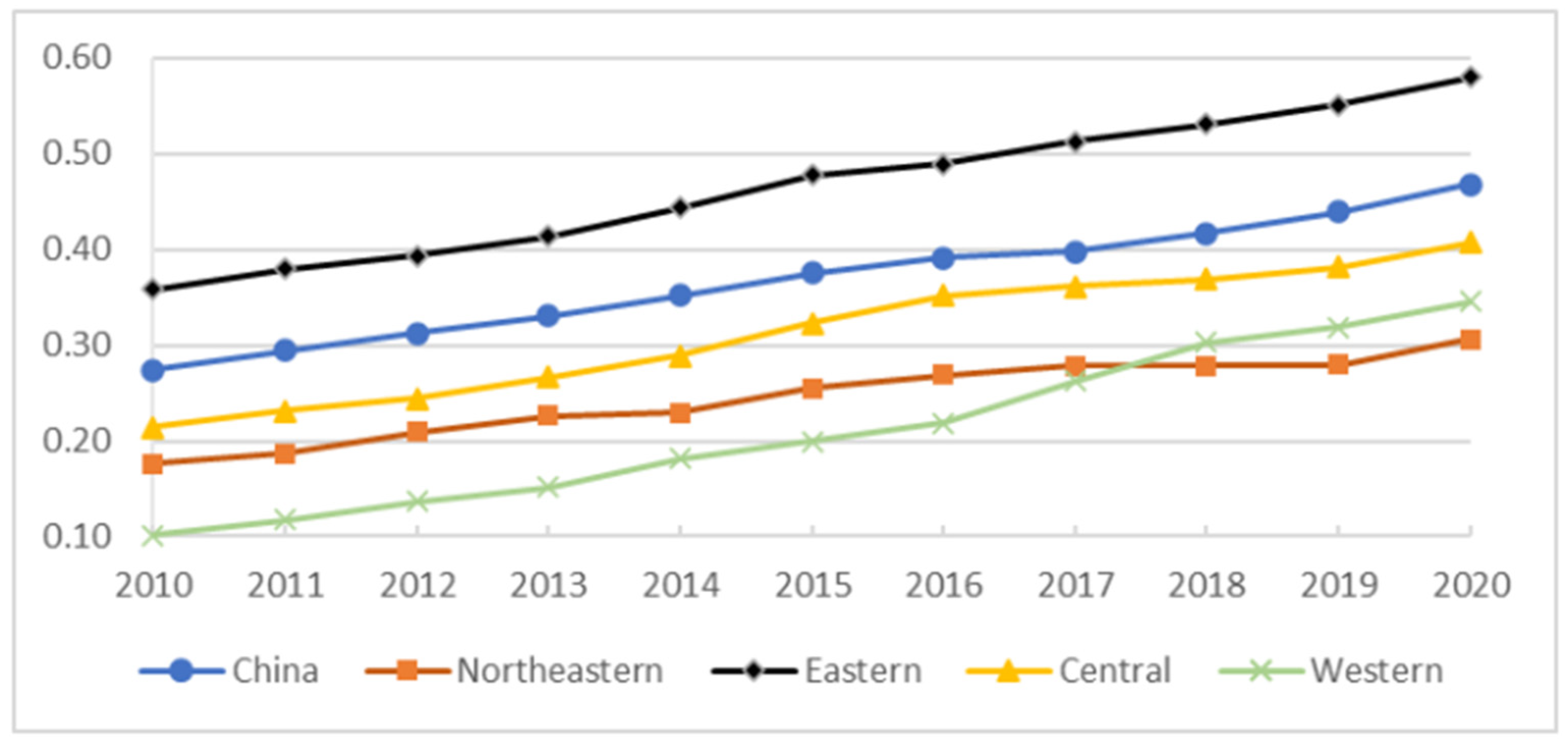
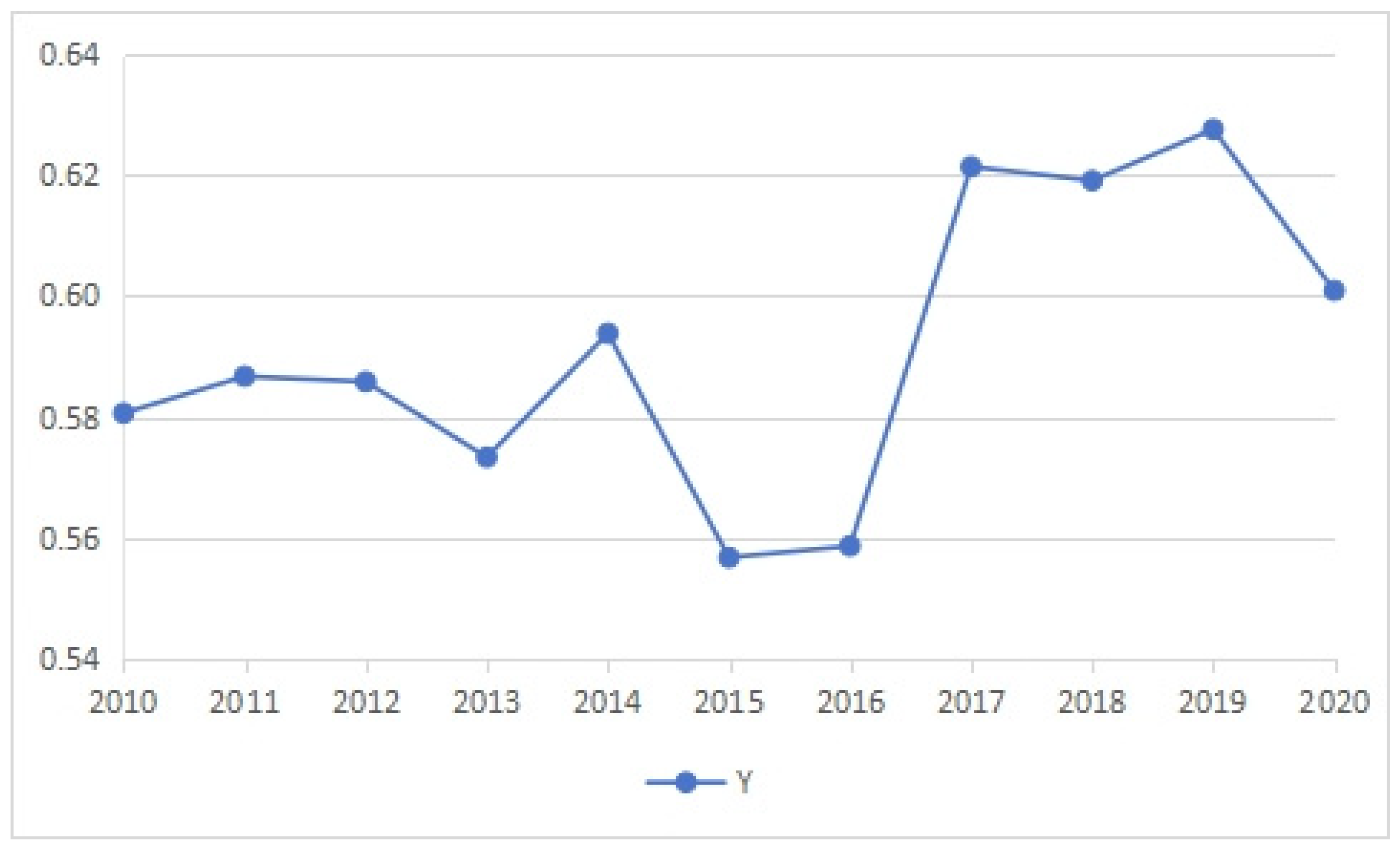
6.2. Temporal Characteristics of the RR Index

6.2.1. Temporal Characteristics of the RR Primary Index

Figure 1 illustrates the growth changes in the development level of RR in each province of China in 2011, 2014, 2017, and 2020.

In Figure 1, different colored legends denote different ranges of values, with darker-colored legends denoting larger ranges of values and lighter-colored legends denoting smaller ranges of values. Each province is marked with a color corresponding to its RR level. The color of each province becomes gradually darker, which indicates that the RR level of each province has increased year by year from 2010 to 2020. In addition, colors vary among provinces, indicating that different provinces enjoy different RR levels. For instance, eastern provinces (e.g., Jiangsu, Shanghai, Fujian, and Zhejiang) are marked with much darker colors, which implies that eastern provinces enjoy a higher RR level compared to those of other regions.

The National Bureau of Statistics classifies all places into four regions (eastern, central, western, and northeastern regions) based on their geographic location.

Table 5. The development level of RR at regional and provincial levels in 2020.

Region	Province	RR Index	Ranking	Region	Province	RR Index	Ranking
Eastern	Jiangsu	0.6444	1	Western	Chongqing	0.4435	10
	Shanghai	0.6379	2		Ningxia	0.3895	16
	Fujian	0.6038	3		Tibet	0.3868	17
	Beijing	0.5856	4		Xinjiang	0.3743	18
	Zhejiang	0.5801	5		Sichuan	0.3636	19
	Shandong	0.5754	6		Yunnan	0.3606	20
	Tianjin	0.5414	7		Guizhou	0.3452	22
	Guangdong	0.4229	11		Qinghai	0.3403	23
	Hebei	0.4008	14		Gansu	0.3357	24
	Hainan	0.2712	31		Inner Mongolia	0.3293	25
Central	Anhui	0.4992	8		Guangxi	0.3249	26
	Hubei	0.455	9		Shaanxi	0.3198	27
	Jiangxi	0.4165	12	Northeastern	Jilin	0.3506	21
	Hunan	0.4074	13		Liaoning	0.3066	28
	Henan	0.3971	15		Heilongjiang	0.3032	29
	Shanxi	0.3018	30	China	—	0.4677	—

displays the RR level of each province within the four regions. Note that the overall RR index of China is calculated by summing each province’s RR index with its weight, the latter being its GDP as a share of the national GDP [51].

It is not difficult to see from Table 5 a pecking order of Eastern > China > Central > Western > Northeastern in terms of the RR level. This difference has a lot to do with Real GDP (RGDP). In general, the larger the RGDP, the greater the government’s financial support for the village and the higher the RR level. Consistent with this view,

Table 6. Correlation between the RR level (Y Index) and Real GDP.

	Y	RGDP
Y	1
RGDP	0.532 ***	1

Notes: * p < 0.1, ** p < 0.05, *** p < 0.01.

shows a significant positive correlation between the RR level (Y Index) and the RGDP in each province.

To ease the job of understanding the variations in this characteristic in detail from 2010 to 2020, we follow a practice that is commonly used in economic geography by selecting a province that ranks at or near the median of the RR index in each region as the representative province for that region. Specifically, Zhejiang has been chosen for the eastern region, Hunan for the central region, Guizhou for the western region, and Liaoning for the northeastern region. Then, we compare the RR indexes of the four provinces (or regions) and China.

Figure 2 shows that the RR levels of the four regions and China have been on the rise annually. The RR level of the western region began to accelerate in 2016, while the RR indexes of the other three regions slowed after 2016. Since 2018, the RR index of the western region has surpassed that of the northeastern region.

Figure 2 also shows that the COVID-19 pandemic had no large negative impact on the RR levels in China and four economic regions. This is mainly because when the COVID-19 pandemic broke out in December 2019, China took effective city lockdown measures to bring the pandemic under control in a short time. In April 2020, the lockdown measures were lifted, and work and production gradually resumed. Therefore, the pandemic did no large harm to the RR in China. In fact, the RR level in 2020 increased compared to 2019.

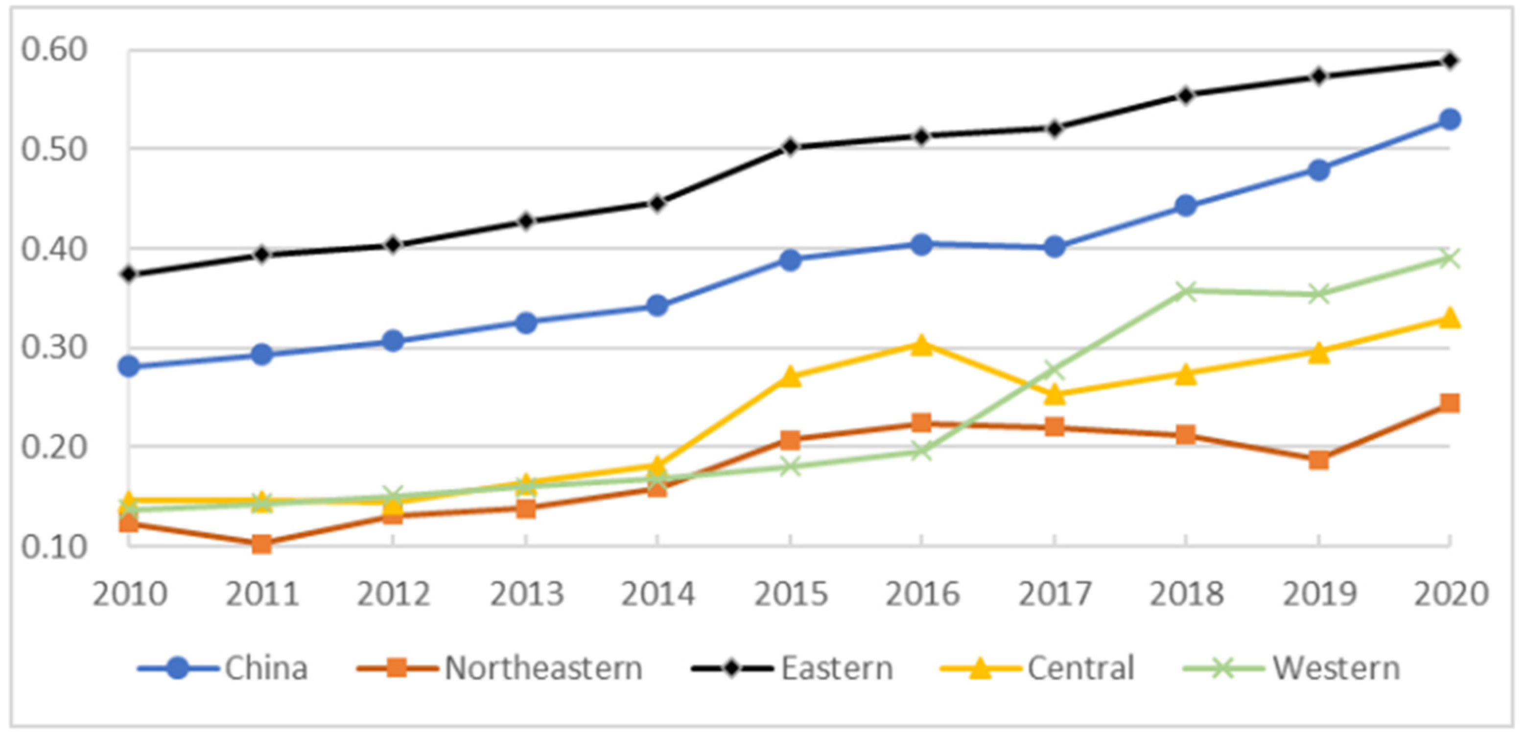
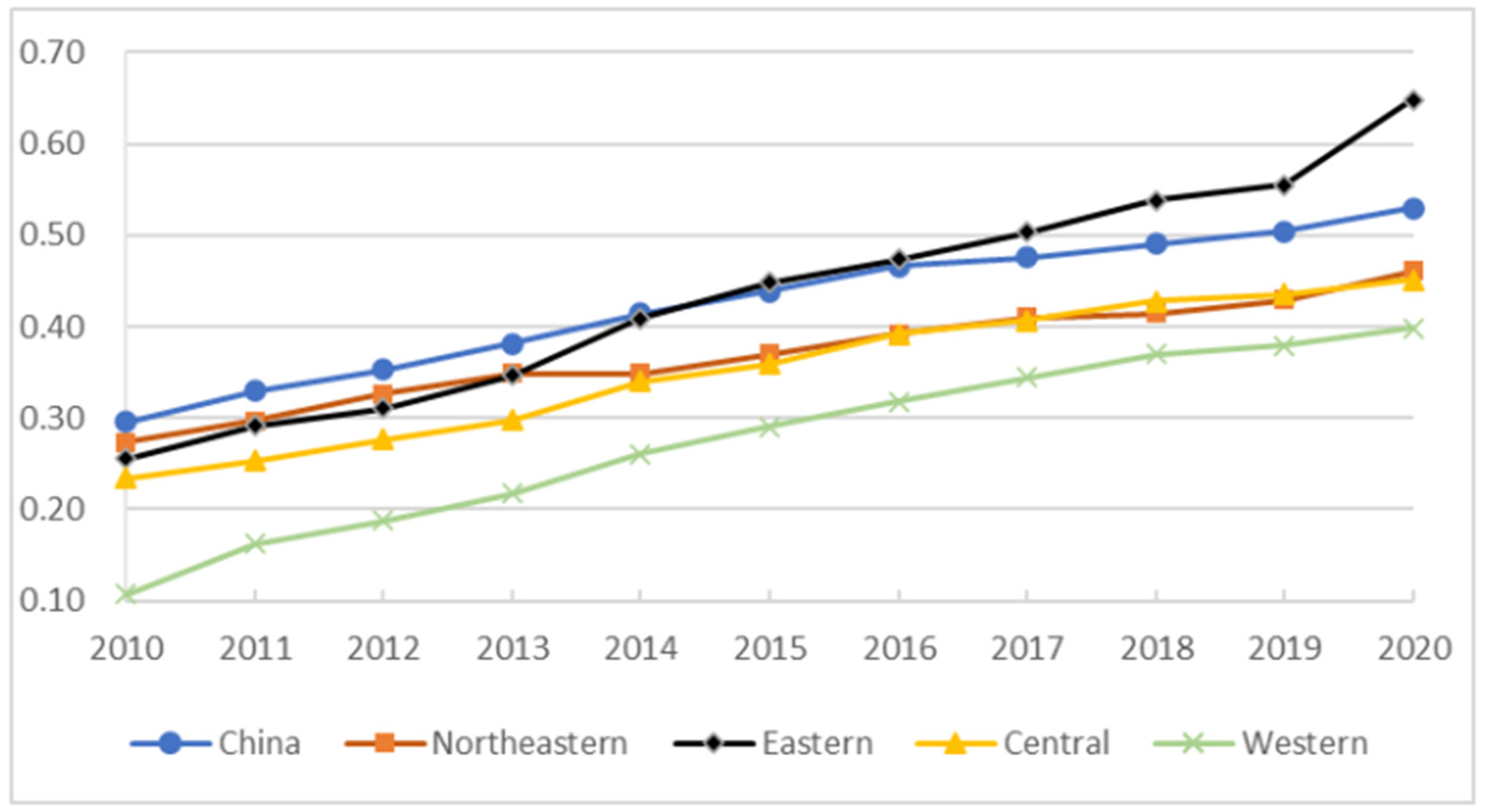
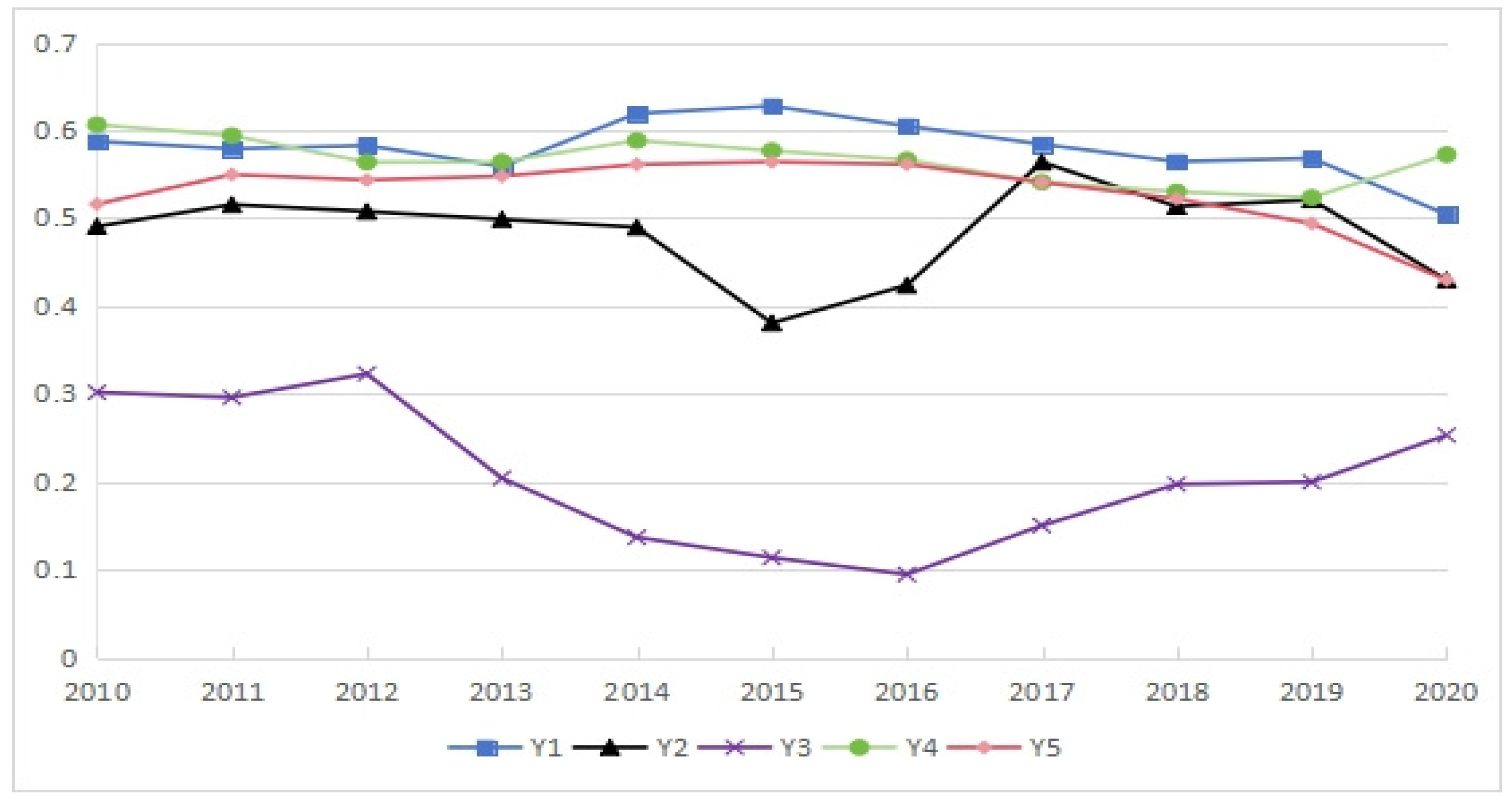
6.2.2. Temporal Characteristics of the RR Secondary Indexes

Recall that RR contains five dimensions/secondary indexes, namely, thriving businesses, pleasant living environments, social etiquette and civility, effective governance, and prosperity. Figure 3, Figure 4, Figure 5, Figure 6 and Figure 7 illustrate the time series trends of these secondary indexes of RR for the four economic regions and China as a whole.

The thriving businesses (Y1) index (see Figure 3) shows that the eastern and central regions are above the national average, while the northeastern and western regions are below the national average. Compared with 2010, the gap between the thriving businesses indexes among the four economic regions in 2020 has narrowed. From 2010 to 2020, rural industries in the eastern and northeastern regions developed slowly and declined in 2014 and 2016; however, rural industries in the central and western regions have developed favorably and grown steadily, catching up with the eastern and northeastern regions.

Figure 4 shows that the gap between the four economic regions, measured in terms of the pleasant living environments (Y2) index, is widening, with the gap between the eastern and northeastern regions being 0.25 in 2010, and this gap widening to 0.35 by 2020. The reason is that the northeastern region saw a decline in the Y2 index, while the eastern region continued to see a steady increase in the Y2 index from 2016 onwards. The Y2 index in the central region also enjoyed a moderate growth rate. Meanwhile, the Y2 index of the western region has experienced an accelerated rise since 2016, approaching the national average. This rise contributed to a sudden increase in the RR primary index (Y) in 2016.

The social etiquette and civility (Y3) index in Figure 5 shows that the Y3 index in the northeastern region has a strong contrast between 2010 and 2020, ranking first in 2010 but last in 2020. This is mainly because the growth rate of the Y3 index in the northeastern region has been slow, far less than that of the other three regions over the past 10 years. The western region has the fastest growth rate, a sharp rise of 242% from 2010 to 2020, followed by Zhejiang (182%), Hunan (151%), and Liaoning (56.8%). The gap between the Y3 indexes of the four economic regions has exhibited a trend of divergence since 2014.

Figure 6 reveals that the effective governance (Y4) indexes of the four economic regions have grown steadily over the past 10 years, and the gap between indexes has not changed notably except for that of Zhejiang in 2020. It is worth noting that, the national average of effective governance is higher than that of the four economic regions from 2010 to 2013, indicating that the distribution of effective governance data is right-skewed in these years.

Figure 7 depicts that the trend of the prosperity (Y5) index is closest to that of the RR primary index (Y). They share similar features: Eastern > China > Central > Northeastern > Western. The Y5 indexes of the four economic regions and China as a whole have increased at a modest pace with a faster growth in the eastern and western regions and a slower growth in the central and northeastern regions. The gap among different regions has not changed significantly.

Table 7. Ranking of China and its regions in terms of the RR primary and secondary indexes.

Region	Y	Y1	Y2	Y3	Y4	Y5
Northeastern	5	4	5	5	3	5
Eastern	1	2	1	1	1	1
Central	3	1	4	3	4	3
Western	4	5	3	2	5	4
China	2	3	2	4	2	2

summarizes the ranking results of the primary and secondary indexes from Figure 2, Figure 3, Figure 4, Figure 5, Figure 6 and Figure 7 for 2020. It is clear from Table 6 that the ranking of the primary index can be different from that of the secondary index in the same region. Take the central region as an example. The primary index is 3 but the secondary indexes range from 1 to 4, respectively. The difference is because different weights are allocated to different secondary indexes and their contribution to the primary index varies (see

Table 8. Contribution of the secondary index to the primary index.

Secondary Index	Y1	Y2	Y3	Y4	Y5
Contribution	20.70%	26.37%	12.23%	15.91%	24.78%

). Thus, it could be misleading to look at the primary index alone. Rather, it is important to examine the primary index together with the secondary indexes to identify what dimension(s) of rural revitalization can be improved.

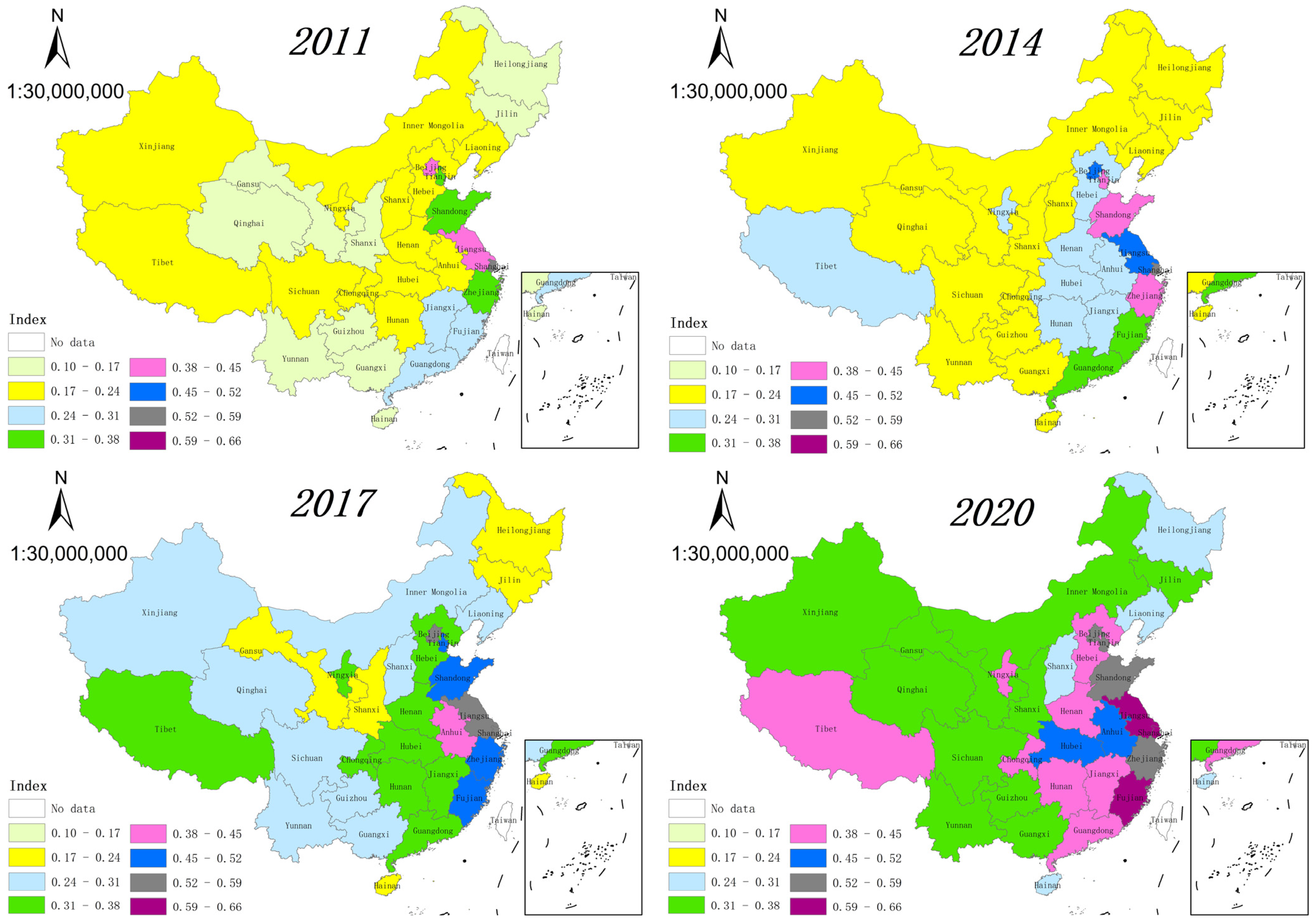
6.3. Spatial Characteristics of the RR Index

6.3.1. Spatial Characteristics of the RR Primary Index

1.

Global characteristics

To show the overall spatial clustering of the RR primary index (Y), we conducted a global spatial correlation test on the index at the provincial level from 2010 to 2020. The test results are shown in

Table 9. The spatial correlation test on the Y index from 2010 to 2020.

Year	I	E(I)	sd(I)	z	p-Value
2010	0.581	−0.033	0.115	5.351	0.00 ***
2011	0.587	−0.033	0.115	5.370	0.00 ***
2012	0.586	−0.033	0.116	5.342	0.00 ***
2013	0.573	−0.033	0.117	5.204	0.00 ***
2014	0.594	−0.033	0.117	5.349	0.00 ***
2015	0.557	−0.033	0.118	4.987	0.00 ***
2016	0.559	−0.033	0.118	5.003	0.00 ***
2017	0.621	−0.033	0.119	5.511	0.00 ***
2018	0.619	−0.033	0.119	5.464	0.00 ***
2019	0.628	−0.033	0.120	5.529	0.00 ***
2020	0.601	−0.033	0.120	5.306	0.00 ***

Notes: * p < 0.1, ** p < 0.05, *** p < 0.01.

below.

Table 9 shows that values of the Global Moran’s I of the index Y fluctuate around 0.6 (Figure 8 below) during the period of 2010 to 2020; they are all positive and statistically significant at the one-percent level. In other words, the spatial correlation test suggests that the index Y is spatially positively autocorrelated.

There is a sharp decrease in the Global Moran’s I in 2015 and 2016. This is mainly because of the decline in the RR index of Beijing. From 2015 to 2017, Beijing’s RR index first rose and then fell, while the RR indexes of other provinces in general showed a moderate upward trend. The deviation between the upward trend of the indexes of Beijing and other provinces weakened their correlations, resulting in a decline in the Global Moran’s I.

The RR index of Beijing decreased because of a decline of more than 20% in the third-level indicators of X2 (level of agricultural mechanization) and X4 (food crop production per mu). Based on its own urban and rural characteristics of “big city, small agriculture” and “big suburb, small urban area”, Beijing has vigorously developed special agriculture, leisure agriculture, and rural tourism, resulting in the underdevelopment of traditional agriculture and a decline in food crop production.

2.

Local characteristics

We conducted a local spatial correlation test on the RR primary index (Y) of each province from 2010 to 2020 to examine the local spatial clustering of the index Y. The test results in the form of Moran scatterplots are shown in Figure 9 below. It is clear from Figure 9 that the provinces in the eastern region are mostly located in the first quadrant, which represents high–high agglomeration; the northeastern provinces and the provinces in the western region are mostly located in the third quadrant, which represents low–low agglomeration; and the provinces in the central region are mostly located in the fourth quadrant, which represents high–low agglomeration. As far as the significance level is concerned, only those of Shanghai, Jiangsu, and Zhejiang, which lie in the first quadrant representing high–high agglomeration, are significant, while the agglomeration characteristics of the rest provinces are not significant.

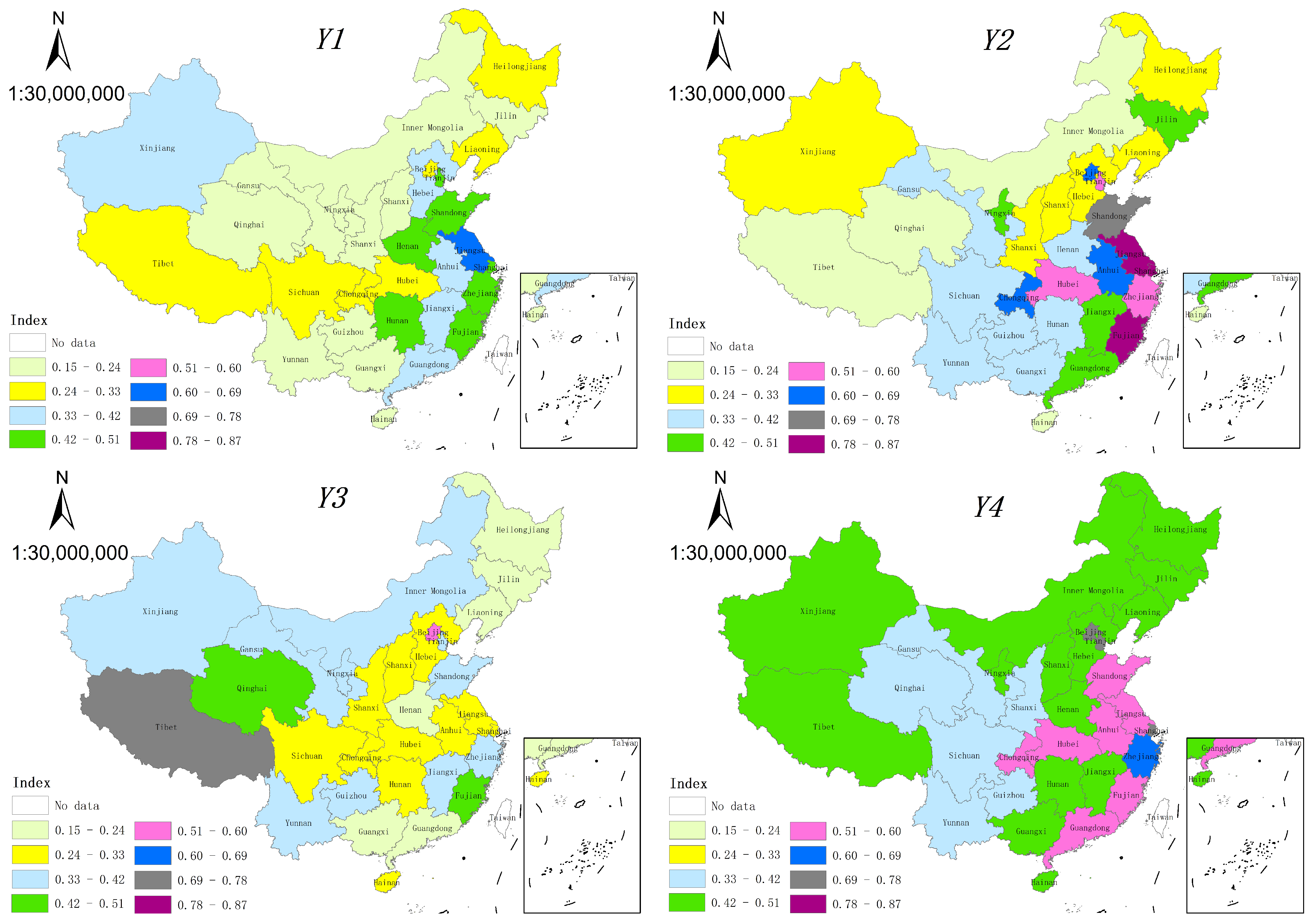
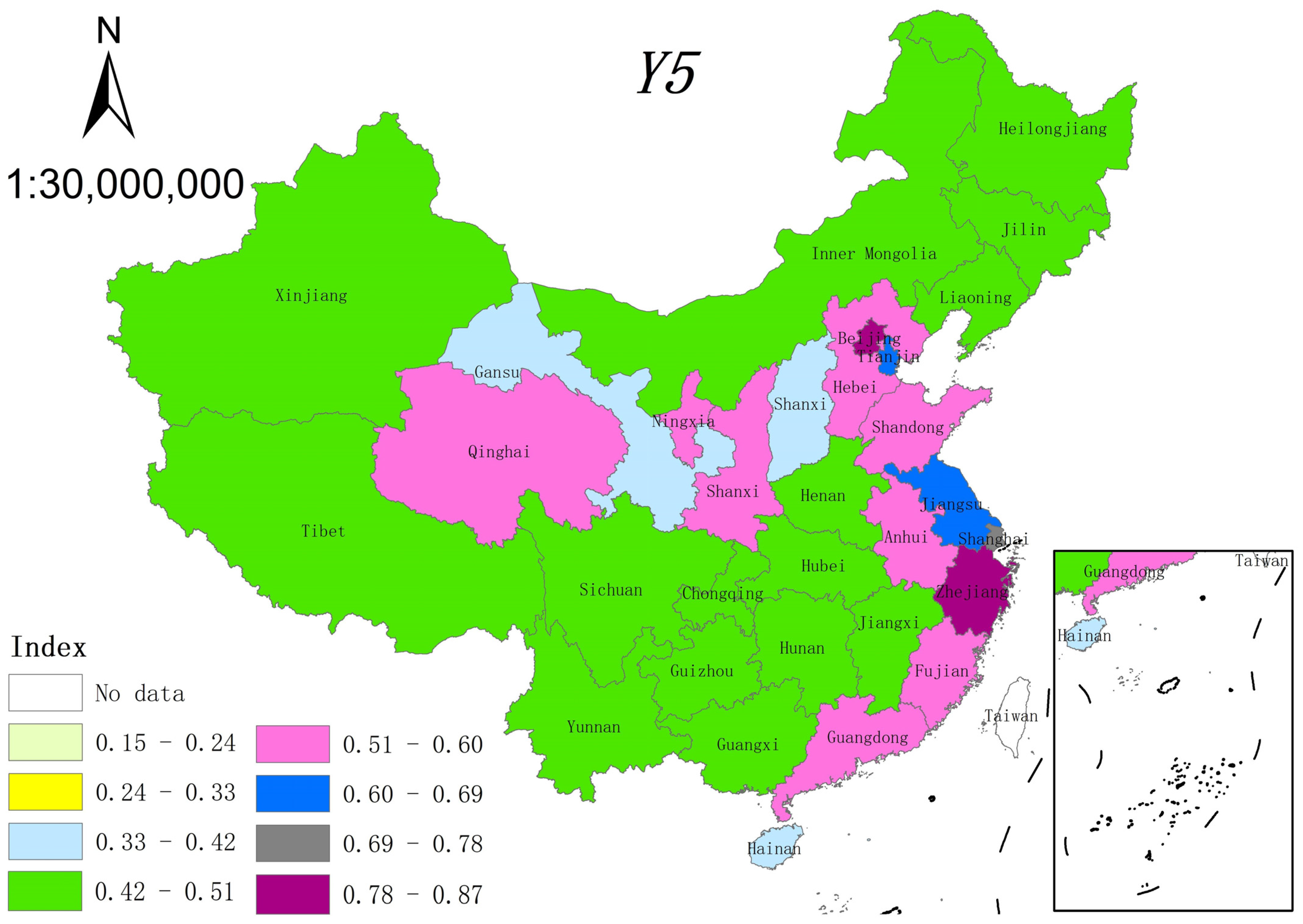
6.3.2. Spatial Characteristics of the RR Secondary Indexes

1.

Global characteristics

We conducted a similar global spatial correlation test on each of the RR secondary indexes (Y1, Y2, Y3, Y4, and Y5) at the provincial level from 2010 to 2020. The test results are shown in Figure 10. All the values of the Global Moran’s I are positive, suggesting that these secondary indexes also exhibit spatial clustering. Figure 10 shows that Y1 has the strongest agglomeration, but it began to gradually decline after peaking in 2015. A close look at the trend in changes in the Y1 index of each province reveals that the provincial discrepancy in the Y1 index was on the decrease before 2015, and then began to widen after 2015. Consequently, the value of Global Moran’s I of the index Y reached its peak in 2015. A possible explanation is that the cross-sectional variations in the Y1 index may be related to the macroeconomic situation in China. After 2015, China’s GDP growth rate fell below 7% and declined year after year. During the macroeconomic downturn, due to the different resilience of the rural industries in each province, the discrepancies in the Y1 index were enlarged compared to the macroeconomic boom period. Whether rural industries are thriving or not is a precondition for whether farmers’ lives are affluent or not. They are closely correlated. This explains why the Y5 index exhibits similar spatial agglomeration characteristics to those of the Y1 index.

Figure 10 shows that the agglomeration of the Y4 index dwindled in 2015, but suddenly rose in 2020. The reason is that Zhejiang and Gansu witnessed a relatively large increase in the Y4 index in 2020, narrowing the gap between these provinces and other provinces. This increase came from a sharp rise of more than 50% in the third-level indicator of X18 (proportion of party members among village directors) of each province in 2020. The sharp rise is associated with the adoption of the Several Opinions of the State Council on Adhering to the Priority Development of Agriculture and Rural Areas and Addressing Well the Issues Relating to Agriculture, Rural Areas and Rural People by the State Council in January 2019, which explicitly states that governments should raise the proportion of party members among members of village committees and villagers’ deputies, and strengthen the leadership of party branches over village collective economic organizations.

Figure 10 also shows that the Y3 index has the weakest agglomeration. This is easy to understand. The Y1 index has the strongest agglomeration because economic exchanges among provinces are the most frequent. In contrast, the Y3 index has the weakest agglomeration because cultural exchanges among provinces are relatively sparse. The agglomeration of the Y2 index displayed a drop–rise–drop oscillatory trend during the study period, fluctuating narrowly and irregularly around the horizontal line of 0.5.

2.

Local characteristics

The RR secondary index includes the Y1, Y2, Y3, Y4, and Y5 indexes, whose local spatial characteristics are similar to those of the RR primary index, and thus the analysis will not be repeated.

6.4. Driving Factors of RR

6.4.1. The Strategy of RR

China has been implementing the RR strategy since 2017. To study the effect of the strategy, we compare the changes in the mean and standard deviation of the RR index between two periods before and after 2017, i.e., 2013–2016 and 2017–2020 (see

Table 10. The changes in the mean and standard deviation of RR primary index Y and RR secondary indexes Y1, Y2, Y3, Y4, and Y5.

	2013–2016		2017–2020		2017–2020/2013–2016		2017–2020/2013–2016
	Mean	Std. Dev.	Mean	Std. Dev.	Difference in Mean	p-Value	Difference in Std. Dev.	p-Value
Y1	0.279	0.133	0.296	0.126	0.017 (5.99%)	0.155	−0.007 (−5.42%)	0.269
Y2	0.263	0.169	0.373	0.199	0.110 (41.59%)	0.000 ***	0.030 (17.93%)	0.034 **
Y3	0.226	0.085	0.310	0.107	0.084 (37.20%)	0.000 ***	0.022 (26.13%)	0.005 ***
Y4	0.373	0.089	0.469	0.096	0.096 (25.61%)	0.000 ***	0.007 (8.01%)	0.197
Y5	0.368	0.126	0.498	0.124	0.129 (35.10%)	0.000 ***	−0.002 (−1.60%)	0.429
Y	0.296	0.108	0.379	0.113	0.084 (28.25%)	0.000 ***	0.005 (4.13%)	0.327

Notes: * p < 0.1, ** p < 0.05, *** p < 0.01.

).

Table 10 shows the changes in the mean and standard deviation of the RR primary and secondary indexes between the periods 2013–2016 and 2017–2020. On the one hand, the mean values of the RR primary and secondary indexes have risen by varying degrees after the implementation of the RR strategy, which means that the strategy has contributed to an increase in the development level of RR; on the other hand, there is a decrease in the standard deviation of Y1 and Y5 and an increase in the standard deviation of Y2, Y3, Y4, and Y, respectively. Moreover, differences in the standard deviation of Y2 and Y3 are large and significant, which increase by 17.93% and 26.13%, respectively. This suggests that the development imbalance among China’s regions has not been entirely improved after the implementation of the RR strategy and that gaps among provinces in terms of Y2 and Y3 are instead widening, which deserves local governments’ attention.

6.4.2. Five Secondary Indexes

The RR primary index Y covers five dimensions, i.e., Y1–Y5. To examine the impact of each dimension on the Y index in a detailed and visual way, we have produced a radar chart showing RR performance in five dimensions for four representative provinces in the eastern, central, western, and northeastern regions of China: Zhejiang, Hunan, Guizhou, and Liaoning.

As can be seen from Figure 11, Zhejiang scores highest on all five secondary indexes, while Liaoning, on the inner side, scores lowest, especially in the Y2 and Y3 indexes. Hunan and Guizhou score in the middle of the ranking. These differences should be taken into account when formulating effective RR policies, as a one-size-fits-all approach may not be suitable for every province.

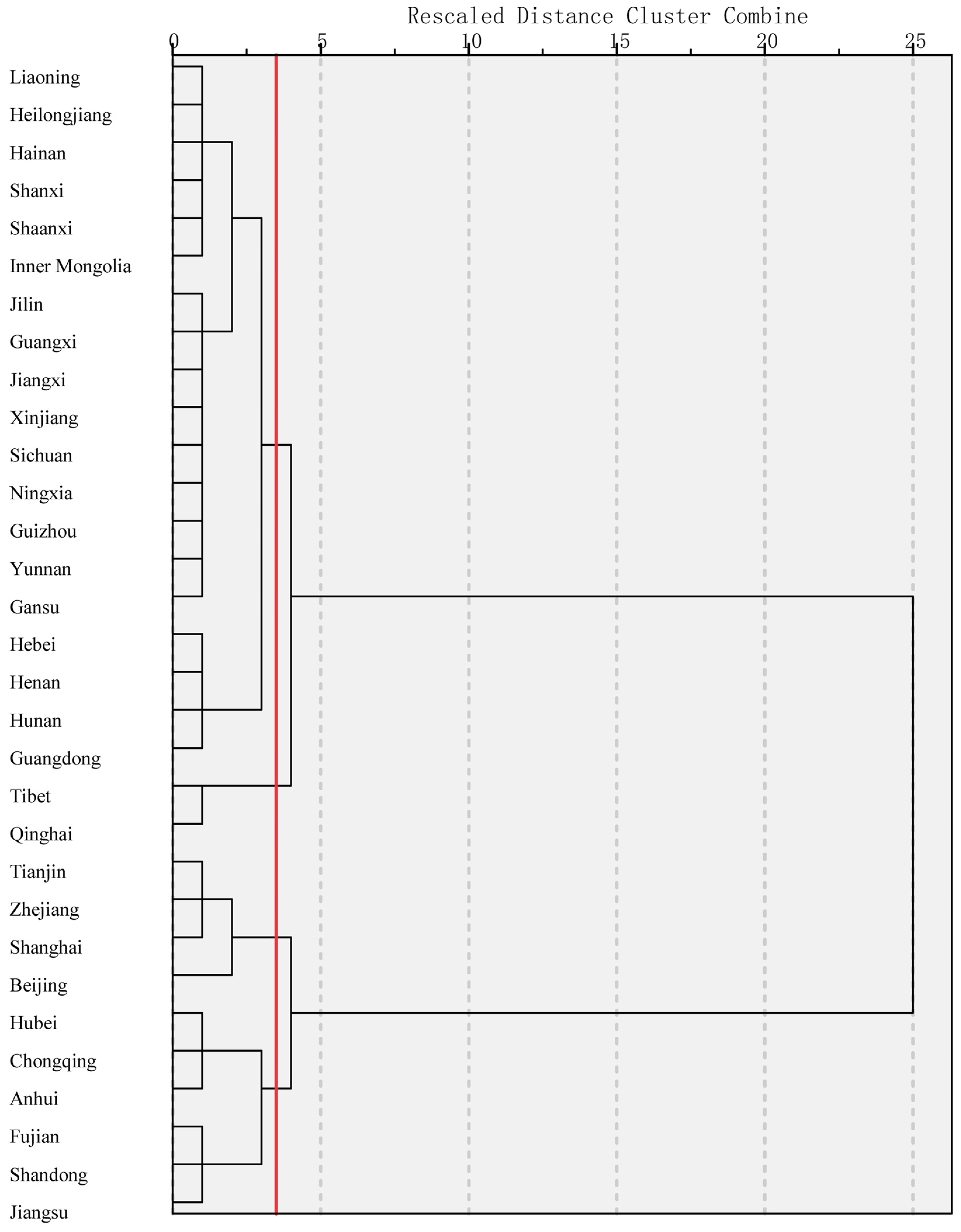
6.5. Cluster Analysis

6.5.1. Ward Clustering Results

The RR primary index measures the overall development level of RR in a province, but it cannot reveal the development status of the five secondary indexes underlying it. In fact, there are remarkable variances in the five RR secondary indexes among provinces, and Figure 12 visualizes the variances among provinces in 2020.

In Figure 12, different colored legends denote different ranges of values, with darker-colored legends denoting larger ranges of values and lighter-colored legends denoting smaller ranges of values. Taking the top-left secondary index Y1 as an example, Jiangsu’s Y1 index for 2020 has a value of 0.623 and is thus labeled blue; Hubei’s Y1 index for 2020 has a value of 0.325 and is thus labeled yellow; Hunan’s Y1 index for 2020 has a value of 0.467 and is thus labeled green; and the other provinces are labeled with a color corresponding to the legend. Overall, the color of the eastern provinces is darker than that of the western provinces, showing that the eastern provinces perform better than the western provinces on the RR secondary index. And, it is easy to find that there is a significant variance in the Y1 index among provinces. Moreover, the other four graphs in Figure 12 show that there is also a significant variance in the Y2–Y5 indexes of each province.

Notwithstanding the remarkable variances mentioned above, the five secondary indexes are highly correlated (see

Table 11. The correlation coefficients for the RR secondary indexes.

	Y1	Y2	Y3	Y4	Y5
Y1	1
Y2	0.696 ***	1
Y3	0.064	0.266 ***	1
Y4	0.601 ***	0.722 ***	0.467 ***	1
Y5	0.588 ***	0.736 ***	0.590 ***	0.885 ***	1

Notes: * p < 0.1, ** p < 0.05, *** p < 0.01.

below). Table 11 shows that except for the correlation coefficient of Y1 and Y3, which is not significant, all the other correlation coefficients are positive and statistically significant at the one-percent level. This reveals an interesting latent fact that the five dimensions of RR are interconnected and they influence and interact with each other [52], confirming that they are five indispensable components of RR. Thus, in the process of comprehensively promoting RR, none of these aspects should be overlooked.

We also conduct a Ward cluster analysis on the RR secondary indexes at the provincial level. Thirty-one provinces are clustered into four categories and seven subcategories (see Figure 13 and

Table 12. Clustering results of the secondary indexes of RR.

Category	Subcategory	Province	Region	Ranking	Category	Subcategory	Province	Region	Ranking
First	1	Beijing	Eastern	4	Fourth	6	Gansu	Western	24
		Shanghai	Eastern	2			Yunnan	Western	20
		Zhejiang	Eastern	5			Guizhou	Western	22
		Tianjin	Eastern	7			Ningxia	Western	16
Second	2	Jiangsu	Eastern	1			Sichuan	Western	19
		Shandong	Eastern	6			Xinjiang	Western	18
		Fujian	Eastern	3			Jiangxi	Central	12
	3	Anhui	Central	8			Guangxi	Western	26
		Chongqing	Western	10			Jilin	Northeastern	21
		Hubei	Central	9		7	InnerMongolia	Western	25
Third	4	Qinghai	Western	23			Shaanxi	Western	27
		Tibet	Western	17			Shanxi	Central	30
Fourth	5	Guangdong	Eastern	11			Hainan	Eastern	31
		Hunan	Central	13			Heilongjiang	Northeastern	29
		Henan	Central	15			Liaoning	Northeastern	28
		Hebei	Eastern	14			-	-	-

). Each subcategory entails a different development focus.

The column ‘Region’ shows that provinces located in the same region are mostly classified into one category. However, there are some exceptions. Subcategories 3–7 contain provinces in different regions and the RR levels of provinces in the same subcategory are close. Hence, this suggests that following the National Bureau of Statistics’ classification of eastern, central, western, and northeastern regions based on the geographic location of provinces may not capture the RR effectively.

The column ‘Ranking’ shows a similar pattern. In particular, provinces with close rankings are mostly classified into one category, yet with a few exceptions. As the Ward method performs clustering analysis based on the proximity of the secondary indexes of RR of each province rather than the ranking order of the RR primary index, it does not group Jiangsu, Shanghai, Fujian, and Beijing into one category. Thus, it is a more accurate and meticulous classification method.

6.5.2. Analysis and Policy Implications

Following Wang and Wang [53], Wang et al. [54], and Ju et al. [55], we analyze the clustering results as follows.

The first category contains four provinces, Beijing, Shanghai, Zhejiang, and Tianjin, and the primary indexes of RR (Y) in the four provinces are at the forefront of the country (see

Table 13. Ranking of provinces in the first category in terms of the RR primary and secondary indexes.

Province	Y1	Y2	Y3	Y4	Y5	Y
Beijing	17	7	2	2	1	4
Shanghai	4	3	17	1	3	2
Zhejiang	6	9	5	4	2	5
Tianjin	7	10	10	3	4	7

below). The Y4 and Y5 indexes of the four provinces occupy the top four places in terms of their rankings, contributing most to the overall level of RR, respectively, which is measured by the Y index. Beijing’s Y1 index rank is low, at 17th place, because of the low food crop production per mu (X4) and village industrial investment (X5), which are only about 50 percent of their counterparts in Shanghai. The reason for the lower Y3 index in Shanghai and Tianjin is that village social custom (X16) scores lower, which are equivalent to about 50% and 60% that of Beijing, respectively. Zhejiang and Tianjin have lower scores in domestic sewage disposal rate (X11), and non-hazardous disposal rate of domestic waste (X12), resulting in their relatively low rankings in the Y2 index.

Therefore, when promoting the development level of RR, Beijing is expected to pay attention to the development of rural industries; Shanghai is expected to pay attention to the development of rural culture; Zhejiang is expected to pay attention to the control of rural environmental pollution; and Tianjin is expected to pay attention to both the development of rural culture and the protection of rural environmental at the same time.

The second category, including the six provinces of Jiangsu, Shandong, Fujian, Anhui, Chongqing, and Hubei, is subdivided into two subcategories (see

Table 14. Ranking of provinces in the second category in terms of the RR primary and secondary indexes.

Province	Y1	Y2	Y3	Y4	Y5	Y
Jiangsu	1	1	18	5	5	1
Shandong	3	4	8	8	6	6
Fujian	2	2	4	6	10	3
Anhui	10	5	21	7	12	8
Chongqing	19	6	23	11	19	10
Hubei	14	8	22	10	15	9

below). Among them, the first three provinces belong to subcategory 2, with a very high overall level of RR; the latter three provinces belong to subcategory 3, with a relatively high overall level of RR.

In subcategory 2, the number of village cultural stations (X15) and village social customs (X16) have brought down Jiangsu’s ranking in the Y3 index (ranking 18th), which is the focus of Jiangsu province’s efforts to promote RR. The Y3 and Y4 indexes are weak and constraining RR in Shandong province. Accordingly, it may be a good idea for Shandong province to strive to increase the number of village cultural stations (X15), reduce the village illiteracy rate (X14), and improve the minimum subsistence allowance per capita (X23). Fujian province has a low score on the Y5 index. The reason is that the number of private cars owned in rural areas (X28) is relatively low, and Fujian province may put more effort into improving the material living standard of rural people.

In subcategory 3, Anhui, Chongqing, and Hubei, ranked lower in the Y1 index, Y3 index, and Y5 index, compared with the Y2 index and Y4 index. Therefore, in the process of implementing the RR strategy, they are expected to increase the focus on reviving rural industries and achieving common prosperity for rural residents, while carrying forward excellent traditional culture and improving people’s ideological and moral standards at the same time.

Table 13 and Table 14 also show that Zhejiang and Jiangsu rank high on the Y5 index respectively. This is related to the good development of rural tourism in these two provinces. According to research by ASKCI Consulting Co., Ltd, the number of key villages for rural tourism in Zhejiang and Jiangsu is 40 and 39, respectively. Rural tourism can increase farmers’ income, which in turn improves the Y5 index.

The third category includes Qinghai and Tibet provinces (see

Table 15. Ranking of provinces in the third category in terms of the RR primary and secondary indexes.

Province	Y1	Y2	Y3	Y4	Y5	Y
Qinghai	29	29	3	26	7	23
Tibet	15	30	1	16	14	17

below), and their rankings in the overall level of RR are slightly below the national average. The two provinces have high scores in the Y3 index due to a great number of village cultural stations (X15), but their scores for the other four secondary indexes are all low. In particular, Qinghai’s Y1 index (ranking 29th), Y2 index (ranking 29th), and Y4 index (ranking 26th), all rank near the bottom of the country. Thus, Qinghai may consider paying more attention to enhancing the level of agricultural mechanization (X2), food crop production per mu (X4), and level of medical services (X22) in the process of comprehensively promoting RR. Tibet’s Y2 index also ranks extremely low; therefore, strengthening the treatment of rural environmental pollution (involving the third-level indicators X11 and X12) is something that both Qinghai and Tibet may consider to accomplish RR.

The fourth category, comprising 19 provinces, is subdivided into three subcategories (see

Table 16. Ranking of provinces in the fourth category in terms of the RR primary and secondary indexes.

Province	Y1	Y2	Y3	Y4	Y5	Y
Guangdong	12	12	27	9	9	11
Hunan	5	21	15	21	22	13
Henan	8	20	29	12	21	15
Hebei	9	22	24	13	8	14
Gansu	30	15	12	28	30	24
Yunnan	25	18	6	27	16	20
Guizhou	31	16	9	30	23	22
Ningxia	22	13	13	22	11	16
Sichuan	16	17	20	29	17	19
Xinjiang	13	23	7	23	24	18
Jiangxi	11	14	11	15	20	12
Guangxi	24	19	28	18	27	26
Jilin	28	11	30	24	25	21
InnerMongolia	21	28	14	14	18	25
Shaanxi	26	24	19	31	13	27
Shanxi	27	25	16	25	29	30
Hainan	23	31	25	17	31	31
Heilongjiang	18	26	31	20	28	29
Liaoning	20	27	26	19	26	28

below). Among them, Guangdong, Hunan, Henan, and Hebei belong to subcategory 5, which ranks slightly above the national average level of RR; Gansu, Yunnan, Guizhou, Ningxia, Sichuan, Xinjiang, Jiangxi, Guangxi, and Jilin belong to subcategory 6, which ranks much lower in terms of the overall level of RR; and Inner Mongolia, Shaanxi, Shanxi, Hainan, Heilongjiang, and Liaoning belong to subcategory 7, which ranks at the bottom of the overall level of RR.

In subcategory 5, Guangdong is the largest economic province in China, with the highest GDP across the country, but its ranking on the Y1 index relatively lags, suggesting that it has focused more on the development of cities than villages in the past. So, it may consider paying more attention to the construction of the rural economy in the process of promoting RR in the years ahead. The Y3 index of Guangdong, Hunan, and Hebei ranks 27th, 29th, and 24th, respectively. These low rankings are correlated with the low score of village social custom (X16) and insufficient investment in the construction of public buildings in villages. The Y5 index of Hunan and Henan ranks 14 and 13 places behind that of Hebei, respectively. This is because Hunan’s rural tap water coverage (X30) is 28 percentage points lower than Hebei’s, and Henan’s growth rate of real income of farmers (X25) is 2 percentage points lower than Hebei’s. These three provinces all have a relatively low Y2 index ranking due to the low scores of the domestic sewage disposal rate (X11) indicator. The deficiencies or lagging of the above indicators could be the focus of improvements during the process of implementing the RR strategy in the corresponding provinces.

In subcategory 6, all provinces rank modestly well on the indexes Y2 and Y3 but lag on the other three indexes. Gansu, Yunnan, Guizhou, Ningxia, Guangxi, and Jilin lag on index Y1; Gansu, Yunnan, Guizhou, Ningxia, Sichuan, Xinjiang, and Jilin lag on index Y4; and Gansu, Guizhou, Xinjiang, Guangxi, and Jilin lag behind on the index Y5. A closer analysis of the third-level indicators reveals that provinces lagging on the Y1 index may consider improving the level of irrigated farmland (X3) and the food crop production per mu (X4); provinces lagging on the Y4 index may put more efforts into improving rural medical services level (X22) and minimum subsistence allowance per capita (X23); and provinces lagging on the Y5 index may pay more attention to improving real consumption of farmers (X26) and improving rural living area (X29).

In subcategory 7, all provinces rank relatively poorly on all five secondary indexes. Inner Mongolia, Shaanxi, Shanxi, and Hainan lag on the index Y1; all provinces lag on the index Y2; Hainan, Heilongjiang, and Liaoning lag on the index Y3; Shaanxi and Shanxi lag on index Y4; and Shanxi, Hainan, Heilongjiang, and Liaoning lag on the index Y5. A thoroughly comparative analysis of the third-level indicators suggests that provinces lagging on the Y1 index may put their efforts into improving the level of agricultural mechanization (X2) and the food crop production per mu (X4), and increasing village industrial investment (X5); provinces lagging on the Y2 index may strengthen the control of environmental pollution in rural areas (involving the third-level indicators X11 and X12); provinces lagging on the Y3 index may increase investment in the construction of public buildings in villages, and pass on village social custom (X16); provinces lagging on the Y4 index may increase the proportion of villages that have village development planning (X19) and minimum subsistence allowance per capita (X23); and provinces lagging on the Y5 index may consider increasing the growth rate of real income of farmers (X25) and improving rural living area (X29).

Table 15 and Table 16 also show that Guizhou, Gansu, and Qinghai rank low on the Y1 index respectively. This is related to the decline of agriculture in these three provinces. These three provinces are mountainous and hilly with low rainfall, making them unsuitable for crops. Therefore, these provinces have relatively low food crop production per mu (X4), causing them to lag other provinces on the Y1 index ranking.

7. Conclusions

In this study, we propose a new index for the development level of RR based on five aspects, namely, thriving businesses, pleasant living environments, social etiquette and civility, effective governance, and prosperity. Using data from statistical yearbooks as well as the WIND and CEIC databases, we measure the development level of RR of each province in China from 2010 to 2020 with EWM. Then, we detect the temporal and spatial characteristics of the development level of RR through ESDA and identify the disparities in RR among provinces through Ward cluster analysis. Finally, we give suggestions for improving RR for each province. The key findings of the paper are as follows.

Firstly, the overall development levels of RR in China and its provinces increase year by year over the sample period, yet the overall level of RR is still low, with a national average of merely 0.47 in 2020, while the top province, Jiangsu, only scores 0.64. RR development level is highly heterogeneous among provinces. Provinces with a higher development level of RR are mainly located in the eastern region, followed by the central region, and lastly, the northeastern and western regions.

Secondly, at the secondary indexes level, the RR in China and its provinces also increases year by year, yet there exist gaps between secondary indexes. The relationship among the secondary indexes, in terms of the national average is Y5 > Y4 > Y2 > Y1 > Y3. The gap among the four economic regions on the Y1 index is narrowing while that on the Y2 and Y3 indexes are widening, and that on the Y4 and Y5 indexes do not change obviously.

Thirdly, both the RR primary index and secondary index are notably spatially positively autocorrelated. The primary index exhibits diverse agglomeration characteristics in the four economic regions, with high–high agglomeration in the eastern provinces, low–low agglomeration in the northeastern and western provinces, and high–low agglomeration in the central provinces. The secondary index has similar spatial characteristics to those of the primary index. In addition, the Y1 index has the strongest agglomeration characteristic while the Y3 index has the weakest.

Finally, the 31 provinces of China could be clustered into four categories and seven subcategories through Ward cluster analysis on the RR secondary index. Each province in the different subcategories is facing different challenges in the process of RR and entails different development focuses.

The paper contributes to the growing body of literature that focuses on RR as a major driver of a sustainable economy. First, compared with previous studies, the evaluation system in this paper covers as many as 31 third-level indicators. Therefore, it can assess the level of RR in China comprehensively. Second, prior studies have focused more on the RR primary index, while this paper focuses more on the RR secondary indexes. Third, this paper employs a cluster analysis method to analyze the RR secondary indexes of each province, thereby helping provinces to identify where improvements can be made to promote RR.

Our findings have important implications for policymakers and academics. Since there exists heterogeneity in RR level among provinces and a one-size-fits-all approach may not be suitable for every province; local governments should take this into account in making policies to improve RR. Moreover, our findings lend support to the argument that RR for each province is positively autocorrelated. In particular, our paper suggests that a province should interact with its neighbors actively to achieve better RR. For academics, our paper suggests several directions by which future research can extend from our analysis. First, we encourage future research to examine the effect of RR on the well-being of rural individuals. Second, future research could also explore the influence of RR on high-quality economic development at the macro level.

References

1. Liu, Y.; Zang, Y.; Yang, Y. China’s rural revitalization and development: Theory, technology and management. J. Geogr. Sci. 2020, 30, 1923–1942. [Google Scholar] [CrossRef]
2. Han, J. Prioritizing agricultural, rural development and implementing the rural revitalization strategy. China Agric. Econ. Rev. 2020, 12, 14–19. [Google Scholar] [CrossRef]
3. Tan, M.; Liu, Q.; Huang, N. Path Model and Countermeasures of China’s Targeted Poverty Alleviation and Rural Revitalization. Rev. De Cercet. Si Interv. Soc. 2020, 70. [Google Scholar] [CrossRef]
4. Zhang, D.; Gao, W.; Lv, Y. The Triple Logic and Choice Strategy of Rural Revitalization in the 70 Years since the Founding of the People’s Republic of China, Based on the Perspective of Historical Evolution. Agriculture 2020, 10, 125. [Google Scholar] [CrossRef]
5. Briggeman, B.C.; Gray, A.W.; Morehart, M.J.; Baker, T.G.; Wilson, C.A. A new US farm household typology: Implications for agricultural policy. Appl. Econ. Perspect. Policy 2007, 29, 765–782. [Google Scholar]
6. Homolka, J.; Svecova, M. Analysis of financial support influences on management of agricultural enterprises. Agris on-line Pap. Econ. Inform. 2012, 4, 13–20. [Google Scholar] [CrossRef]
7. Kirchweger, S.; Kantelhardt, J.; Leisch, F. Impacts of the government-supported investments on the economic farm performance in Austria. Agric. Econ. /Zemed. Ekon. 2015, 61, 343–355. [Google Scholar] [CrossRef]
8. Zhou, Z.; Zheng, X. A cultural route perspective on rural revitalization of traditional villages: A case study from Chishui, China. Sustainability 2022, 14, 2468. [Google Scholar] [CrossRef]
9. Xie, K.; Zhang, Y.; Han, W. Architectural Heritage Preservation for Rural Revitalization: Typical Case of Traditional Village Retrofitting in China. Sustainability 2023, 16, 681. [Google Scholar] [CrossRef]
10. Lu, Y.; Qian, J. Rural creativity for community revitalization in Bishan Village, China: The nexus of creative practices, cultural revival, and social resilience. J. Rural. Stud. 2023, 97, 255–268. [Google Scholar] [CrossRef]
11. Geng, Y.; Liu, L.; Chen, L. Rural revitalization of China: A new framework, measurement and forecast. Socio-Econ. Plan. Sci. 2023, 89, 101696. [Google Scholar] [CrossRef]
12. Cen, T.; Lin, S.; Wu, Q. How Does Digital Economy Affect Rural Revitalization? The Mediating Effect of Industrial Upgrading. Sustainability 2022, 14, 16987. [Google Scholar] [CrossRef]
13. Jia, J.; Li, X.; Shen, Y. Indicator system construction and empirical analysis for the strategy of rural vitalization. Financ. Econ. 2018, 11, 70–82. [Google Scholar]
14. Wu, R. Measurement of the development level of provincial rural revitalization and analysis of the characteristics of spatial agglomeration. Stat. Decis. 2023, 39, 59–64. [Google Scholar] [CrossRef]
15. Cai, W.; He, W. Research on comprehensive evaluation of development level of China’s rural revitalization. J. Chongqing Univ. 2023, 1, 102–116. [Google Scholar] [CrossRef]
16. Lv, C.; Cui, Y. Rural Vitalization and Development: Evaluation Index System, Regional Disparity and Spatial Polarization. Issues Agric. Econ. 2021, 42, 20–32. [Google Scholar] [CrossRef]
17. Xu, X.; Wang, Y. Measurement, regional difference and dynamic evolution of rural revitalization level in China. J. Quant. Tech. Econ. 2022, 39, 64–83. [Google Scholar] [CrossRef]
18. Zhang, T.; Li, M.; Xu, Y. The construction and empirical study of rural revitalization evaluation index system. Manag. World 2018, 34, 99–105. [Google Scholar] [CrossRef]
19. Guo, X.; Hu, Y. Construction of evaluation index system of rural revitalization level. Agric. Econ. Manag. 2020, 5, 5–15. [Google Scholar]
20. Mao, J.; Wang, L. Construction of Evaluation Index System of Rural Revitalization—Based on the Demonstration of Province Level. Stat. Decis. 2020, 36, 181–184. [Google Scholar] [CrossRef]
21. Wang, J. Digital inclusive finance and rural revitalization. Financ. Res. Lett. 2023, 57, 104157. [Google Scholar] [CrossRef]
22. Wu, J.; Huang, X. Current diagnosis and spatial pattern of China’s rural revitalization—An empirical study on the scale of prefecture-level cities. Econ. Manag. 2020, 34, 48–54. [Google Scholar]
23. Huang, D.; Jiang, J. Spatial-temporal evolution characteristics and influencing factors of rural revitalization in the Yangtze River Economic Belt. Stat. Decis. 2023, 39, 44–49. [Google Scholar] [CrossRef]
24. Zhu, L.; Mei, X.; Xiao, Z. The digital economy promotes rural revitalization: An empirical analysis of Xinjiang in China. Sustainability 2023, 15, 12278. [Google Scholar] [CrossRef]
25. Liu, Z. Study on regional differences, dynamic evolution and spatial convergence of rural revitalization. Stat. Decis. 2023, 39, 73–78. [Google Scholar] [CrossRef]
26. Chen, Y.; Wang, Q.; Huang, H. A study on performance evaluation of county rural revitalization in Fujian province. Fujian Trib. 2019, 9, 182–190. [Google Scholar]
27. Yan, Z.; Wu, F. From Binary Segmentation to Convergence Development—A Study on the Evaluation Index System of Rural Revitalization. Economies 2019, 31, 90–103. [Google Scholar] [CrossRef]
28. Zhang, X.; Zhou, M.; Huang, L.; Zhao, X. Evaluation of the Implementation status of rural revitalization strategy and route optimization: Based on the survey data of Liaoning Province. Issues Agric. Econ. 2020, 2, 97–106. [Google Scholar]
29. Chen, J.; Shi, H.; Lin, Y. Comprehensive evaluation of the development level of rural revitalization in Yangtze River Delta Region. East China Econ. Manag. 2021, 35, 91–99. [Google Scholar] [CrossRef]
30. Song, L.; Bai, Y. Construction of evaluation index system and regional difference decomposition of rural revitalization level. Stat. Decis. 2022, 38, 17–21. [Google Scholar] [CrossRef]
31. Wang, Q.; Zeng, F. Study of Regional Differences and Convergence in the Level of Rural Revitalization in China. J. Guizhou Univ. Financ. Econ. 2023, 41, 99–110. [Google Scholar]
32. Tian, Q.; Che, S.; Jiang, Y. Measurement and evaluation of the development level of rural revitalization and development in Chongqing. J. Chongqing Univ. Technol. 2022, 36, 79–89. [Google Scholar]
33. Wang, F.K.; Du, T.C. Using principal component analysis in process performance for multivariate data. Omega 2000, 28, 185–194. [Google Scholar] [CrossRef]
34. Craig, H. Principal components analysis in stylometry. Digit. Scholarsh. Humanit. 2023, 39, fqad083. [Google Scholar] [CrossRef]
35. Shlens, J. A tutorial on principal component analysis. arXiv 2014, arXiv:1404.1100. [Google Scholar]
36. Labrín, C.; Urdinez, F. Principal component analysis. In R for Political Data Science; Chapman and Hall/CRC: Boca Raton, FL, USA, 2020; pp. 375–393. [Google Scholar] [CrossRef]
37. Cureton, E.E.; D’Agostino, R.B. Factor Analysis: An Applied Approach; Psychology Press: London, UK, 2013. [Google Scholar]
38. Gorsuch, R.L. Factor Analysis: Classic Edition; Routledge: London, UK, 2014. [Google Scholar]
39. Kline, P. An Easy Guide to Factor Analysis; Routledge: London, UK, 2014. [Google Scholar]
40. Zou, Z.; Yi, Y.; Sun, J. Entropy method for determination of weight of evaluating indicators in fuzzy synthetic evaluation for water quality assessment. J. Environ. Sci. 2006, 18, 1020–1023. [Google Scholar] [CrossRef] [PubMed]
41. Su, H.; Zhu, C. Application of entropy weight coefficient method in evaluation of soil fertility. Recent Adv. Comput. Sci. Inf. Eng. Vol. 2012, 3, 697–703. [Google Scholar] [CrossRef]
42. Wang, P.; Qi, M.; Liang, Y.; Ling, X.; Song, Y. Examining the Relationship between Environmentally Friendly Land Use and Rural Revitalization Using a Coupling Analysis: A Case Study of Hainan Province, China. Sustainability 2019, 11, 6266. [Google Scholar] [CrossRef]
43. Fan, S.; Jiang, M.; Sun, D.; Zhang, S. Does financial development matter the accomplishment of rural revitalization? Evidence from China. Int. Rev. Econ. Financ. 2023, 88, 620–633. [Google Scholar] [CrossRef]
44. Tobler, W.R. A computer movie simulating urban growth in the Detroit region. Econ. Geogr. 1970, 46 (Suppl. 1), 234–240. [Google Scholar] [CrossRef]
45. Yao, X.; Zhao, W.; Yang, Z.; Cao, Z.; Wang, D. Spatial-temporal variation characteristics of air quality and its influencing factors of the Beijing-Tianjin-Hebei urban agglomeration based on ward hierarchical clustering. Ecol. Environ. 2021, 30, 340–350. [Google Scholar] [CrossRef]
46. Huo, Y.; He, Y. Research on the urbanization level of Sichuan based on the maximizing deviation and ward system analysis. Soft Sci. 2010, 24, 71–73. [Google Scholar]
47. Yang, Z. Region spatial cluster algorithm based on ward method. China Popul. Resour. Environ. 2010, 1, 382–386. [Google Scholar]
48. Wu, D.; Wu, D. Some problems in comprehensive evaluation of the principal component analysis. Math. Pract. Theory 2015, 45, 143–150. [Google Scholar]
49. Ge, H.; Qian, Y. The impact mechanism and empirical test of digital inclusive financial services for rural revitalization. Mod. Econ. Res. 2021, 5, 118–126. [Google Scholar] [CrossRef]
50. Chen, Y. Research on the mechanism of digital inclusive finance promoting rural revitalization and development. Mod. Econ. Res. 2022, 6, 121–132. [Google Scholar] [CrossRef]
51. Sun, H.; Gui, H.; Yang, D. Measurement and evaluation of the high-quality of China’s provincial economic development. Zhejiang Soc. Sci. 2020, 8, 4–14. [Google Scholar] [CrossRef]
52. Zang, Y.; Yang, Y.; Liu, Y. Understanding rural system with a social-ecological framework: Evaluating sustainability of rural evolution in Jiangsu province, South China. J. Rural Stud. 2021, 86, 171–180. [Google Scholar] [CrossRef]
53. Wang, W.; Wang, C. Evaluation and Spatial Differentiation of High-quality Development in Northeast China. Sci. Geogr. Sin. 2020, 40, 1795–1802. [Google Scholar] [CrossRef]
54. Wang, Y.; Cheng, X.; Yin, P.; Zh, X. Research on Regional Characteristics of China’s Carbon Emission Performance Based on Entropy Method and Cluster Analysis. J. Nat. Resour. 2013, 28, 1106–1116. [Google Scholar] [CrossRef]
55. Ju, X.; Zhang, Y.; Huang, X. Application of Clustering Analysis to the Study of Real Estate Price of Provinces in the Yangtze River Basin. Econ. Geogr. 2013, 33, 79–83. [Google Scholar] [CrossRef]
56. Liu, Q.; Gong, D.; Gong, Y. Index system of rural human settlement in rural revitalization under the perspective of China. Sci. Rep. 2022, 12, 10586. [Google Scholar] [CrossRef] [PubMed]
57. Liu, F.; Wang, C.; Luo, M.; Zhou, S.; Liu, C. An investigation of the coupling coordination of a regional agricultural economics-ecology-society composite based on a data-driven approach. Ecol. Indic. 2022, 143, 109363. [Google Scholar] [CrossRef]
58. Wang, X.; Yang, C.; Liu, T.; Chen, G.; Yue, H. Assessment spatio-temporal coupling coordination relationship between mountain rural ecosystem health and urbanization in Chongqing municipality, China. Environ. Sci. Pollut. Res. 2022, 29, 48388–48410. [Google Scholar] [CrossRef]
59. Chen, K.; Tian, G.; Tian, Z.; Ren, Y.; Liang, W. Evaluation of the Coupled and Coordinated Relationship between Agricultural Modernization and Regional Economic Development under the Rural Revitalization Strategy. Agronomy 2022, 12, 990. [Google Scholar] [CrossRef]
60. Gu, J.; Zheng, J.; Zhang, J. Research on the coupling coordination and prediction of industrial convergence and ecological environment in rural of China. Front. Environ. Sci. 2022, 10, 1014848. [Google Scholar] [CrossRef]
61. Yang, Y.; Bao, W.; Liu, Y. Coupling coordination analysis of rural production-living-ecological space in the Beijing-Tianjin-Hebei region. Ecol. Indic. 2020, 117, 106512. [Google Scholar] [CrossRef]
62. Liu, W.; Zhou, W.; Lu, L. An innovative digitization evaluation scheme for Spatio-temporal coordination relationship between multiple knowledge driven rural economic development and agricultural ecological environment—Coupling coordination model analysis based on Guangxi. J. Innov. Knowl. 2022, 7, 100208. [Google Scholar] [CrossRef]
63. Chen, X. The core of China’s rural revitalization: Exerting the functions of rural area. China Agric. Econ. Rev. 2020, 12, 1–13. [Google Scholar] [CrossRef]
64. Liu, Z.; Jia, S.; Wang, Z.; Guo, C.; Niu, Y. A Measurement Model and Empirical Analysis of the Coordinated Development of Rural E-Commerce Logistics and Agricultural Modernization. Sustainability 2022, 14, 13758. [Google Scholar] [CrossRef]
65. Liu, Y.; Qiao, J.; Xiao, J.; Han, D.; Pan, T. Evaluation of the effectiveness of rural revitalization and an improvement path: A typical old revolutionary cultural area as an example. Int. J. Environ. Res. Public Health 2022, 19, 13494. [Google Scholar] [CrossRef] [PubMed]
66. Wang, Y.; Chen, X.; Sun, P.; Liu, H.; He, J. Spatial-temporal Evolution of the Urban-rural Coordination Relationship in Northeast China in 1990–2018. Chin. Geogr. Sci. 2021, 31, 429–443. [Google Scholar] [CrossRef]
67. Feng, G.; Zhang, M. The coupling coordination development of rural e-commerce and rural revitalization: A case study of 10 rural revitalization demonstration counties in Guizhou. Procedia Comput. Sci. 2022, 199, 407–414. [Google Scholar] [CrossRef]
68. Abreu, I.; Nunes, J.M.; Mesias, F.J. Can rural development be measured? design and application of a synthetic index to Portuguese municipalities. Soc. Indic. Res. 2019, 145, 1107–1123. [Google Scholar] [CrossRef]
69. Gao, X.; Wang, K.; Lo, K.; Wen, R.; Mi, X.; Liu, K.; Huang, X. An evaluation of coupling coordination between rural development and water environment in Northwestern China. Land 2021, 10, 405. [Google Scholar] [CrossRef]
70. Shi, J.; Yang, X. Sustainable Development Levels and Influence Factors in Rural China Based on Rural Revitalization Strategy. Sustainability 2022, 14, 8908. [Google Scholar] [CrossRef]
Figure 1. The development levels of RR of provinces in China in 2011, 2014, 2017, and 2020. Notes: The map is based on standard map no. GS (2019) 1822, downloaded from the Standard Mapping Service website of the National Administration of Surveying, Mapping, and Geographic Information. The same is true of subsequent figures.
Sustainability 16 04574 g001
Figure 2. The RR indexes of the four economic regions and China as a whole from 2010 to 2020.
Sustainability 16 04574 g002
Figure 3. The thriving businesses (Y1) index of the four economic regions and China as a whole from 2010 to 2020.
Sustainability 16 04574 g003
Figure 4. The pleasant living environments (Y2) index of the four economic regions and China as a whole from 2010 to 2020.
Sustainability 16 04574 g004
Figure 5. The social etiquette and civility (Y3) index of the four economic regions and China as a whole from 2010 to 2020.
Sustainability 16 04574 g005
Figure 6. The effective governance (Y4) index of the four economic regions and China as a whole from 2010 to 2020.
Sustainability 16 04574 g006
Figure 7. The prosperity (Y5) index of the four economic regions and China as a whole from 2010 to 2020.
Sustainability 16 04574 g007
Figure 8. Global Moran’s I of the index Y from 2010 to 2020.
Sustainability 16 04574 g008
Figure 9. Moran scatterplots of the index Y in 2011, 2014, 2017, and 2020. Notes: Due to space limitations, only the 2011, 2014, 2017, and 2020 Moran scatterplots are shown.
Sustainability 16 04574 g009
Figure 10. Global Moran’s I of the index Y1, Y2, Y3, Y4, and Y5 from 2010 to 2020.
Sustainability 16 04574 g010
Figure 11. Radar chart of the RR for Zhejiang, Hunan, Guizhou, and Liaoning in 2020.
Sustainability 16 04574 g011
Figure 12. The RR secondary indexes of provinces in China in 2020.
Sustainability 16 04574 g012aSustainability 16 04574 g012b
Figure 13. Clustering results of the secondary indexes of RR. Note: The red line showes that thirty-one provinces are clustered into four categories.
Sustainability 16 04574 g013