Remotely Sensed Changes in Qinghai–Tibet Plateau Wetland Ecosystems and Their Response to Drought

Abstract

Wetland ecosystems in the Qinghai–Tibet Plateau are pivotal for global ecology and regional sustainability. This study investigates the dynamic changes in wetland ecosystems within the Chaidamu Basin and their response to drought, aiming to foster sustainable wetland utilization in the Qinghai–Tibet Plateau. Using Landsat TM/ETM/OLI data on the Google Earth Engine platform, we employed a random forest (RF) method for annual long-term land cover classification. Standardized precipitation evapotranspiration indices (SPEI3, SPEI6, SPEI9, and SPEI12) on different time scales were used to assess meteorological drought conditions. We employed a Pearson correlation analysis to examine the relationship between wetland changes and various SPEI scales. The BFASAT method was used to evaluate the impact of SPEI12 trends on the wetlands, while a cross-wavelet analysis explored teleconnections between SPEI12 and atmospheric circulation factors. Our conclusion is as follows: The wetlands, including lake, glacier, and marsh wetlands, exhibited a noticeable increasing trend. Wetland expansion occurred during specific periods (1990–1997, 1998–2007, and 2008–2020), featuring extensive conversions between wetlands and other types, notably the conversion from other types to wetlands. Spatially, lake and marsh wetlands predominated in the low-latitude basin, while glacier wetlands were situated at higher altitudes. There were significant negative correlations between the SPEI at various scales and the total wetland area and types. SPEI12 displayed a decreasing trend with non-stationarity and distinct breakpoints in 1996, 2002, and 2011, indicating heightened drought severity. Atmospheric circulation indices (ENSO, NAO, PDO, AO, and WP) exhibited varying degrees of resonance with SPEI12, with NAO, PDO, AO, and WP demonstrating longer resonance times and pronounced responses. These findings underscore the significance of comprehending wetland changes and drought dynamics for effective ecological management in the Chaidamu Basin of the Qinghai–Tibet Plateau.

1. Introduction

In recent years, with population growth, economic development, and industrial progress, the emission rate of greenhouse gases has increased, impacting the carbon cycling processes within terrestrial ecosystems [1]. Global warming has become an undeniable reality [2,3]. Wetland ecosystems are a vital component of terrestrial ecosystems, playing a crucial role in regulating runoff, mitigating floods, and improving water quality. They are of paramount importance for maintaining ecosystem stability and preserving biodiversity [4,5,6]. Since 1900, influenced by hydro-meteorological natural factors and human activities, wetland areas have decreased by 50% globally; as a result, monitoring wetland dynamics and exploring the causes of wetland dynamic changes have become essential aspects of wetland research [7,8].

Remote-sensing-based wetland land cover mapping has emerged as an effective means of wetland dynamic monitoring. Studies combine field observation data, high-resolution remote sensing satellite data, visual interpretation, and pixel-based and object-based features to dynamically monitor land cover [9]. In the domain of wetland remote sensing mapping, for instance, Mao et al. [10] constructed a national sample library of various wetland categories, coupled with object-oriented methods, to achieve refined 30 m resolution maps of wetland types in China. Gong et al. [11] utilized Landsat data and automated classification methods to achieve 30 m resolution fine classification maps of wetlands in China for 1990 and 2020. However, single-category land cover datasets cannot explore the transitions between different land cover types and the potential ecological and environmental issues they may raise [12]. In the field of multi-category land cover mapping, Chen et al. [13] used global 30 m Landsat TM5/ETM+/OLI multispectral images and HJ-1 multispectral images, employing the pixel–object–knowledge (POK) classification method to attain land cover maps for the years 2000, 2010, and 2020. Due to its high classification accuracy and resolution, Globe Land 30 (GLC-30 m) has been applied in land cover resource assessment and the evaluation of land cover products [13]. For instance, Zhang et al. [14] assessed the roughness of underlying surfaces in a Yunnan Datuan Mountain wind farm using the 2010 GLC-30 m data, thereby enabling wind energy resource assessment. However, that has limitations in terms of its longer time cycle, which makes it unsuitable for monitoring rapidly changing wetlands. Zhang et al. [15] utilized Landsat TM/ETM+/OLI satellite data from 1984 to 2020, employing the random forest (RF) method on the Google Earth Engine platform to produce a global 30 m refined land surface cover product (GLC_FCS30) for 1985–2020.

While the GLC_FCS30 product has a higher average overall accuracy compared to GLC-30 m, it also provides more diverse land cover types and has a shortened cycle of 5 years [15]. With 29 land surface cover types, this product is often used in the analysis of spatial and temporal change characteristics in regions with diversified land surface vegetation cover. For instance, Wang et al. [16] analyzed the reasons for the mutual conversion between secondary land cover types of farmlands and woodlands based on the 2000–2020 GLC_FCS30 dataset and socioeconomic data from Myanmar. However, there is still a need to address continuous dynamic time series land evolution. To rapidly and accurately analyze the response of land cover to climate change, the European Space Agency has produced the global land cover dataset (ESA_CCI) with a time scale of 1992–2020 [17]. Due to its advantages of having a long time scale, diverse land cover types, and continuous updating, ESA_CCI is widely used in the production of refined land cover type products and long time series dynamic change monitoring in the field of remote sensing mapping [18]. The China Land Cover Database (CLCD) developed by Yang et al. [19] and the CLC_FCS30 training dataset [15] are both extracted from ESA_CCI. However, the spatial resolution of ESA_CCI is 300 m, and uncertainties in land cover types from coarse resolution data may hinder our understanding of the dynamics of time series land cover [18]. Based on all available Landsat data on the Google Earth Engine (GEE) platform, Yang et al. [19] utilized the 1980–2020 China Land Use Data Sets (CLUDs), selected time series invariant sample points combined with the long time series NDVI and Google Earth to filter invariant sample points, producing the CLCD. The CLCD can detect more surface water and impermeable areas and is more suitable for fine-scale environmental and pavement process simulation research [19]. However, China’s mountainous terrain, complex topography, diverse climatic zoning, varied vegetation cover, urban development conditions, and other complexities lead to the varying accuracy of the land cover datasets in different regions [20]. In summary, establishing a regional high-resolution and long time series annual coverage product set is an effective approach to achieve more accurate land resource assessments and precise spatiotemporal change analyses. This is crucial for the response of terrestrial ecosystems to climate change.

The IPCC’s Sixth Assessment Report highlights that global warming has intensified the frequency and intensity of extreme climate events, with significant impacts on agriculture, water resources, and ecological security [21]. Among the most severe meteorological and hydrological disasters, extreme drought events stand out. Drought, characterized by prolonged water deficiency, reflects the comprehensive influence of all climatic factors on an ecosystem [22]. In recent years, regional drought events have become more frequent, such as the autumn drought in Southwestern China in 2003, the spring drought in Yunnan in 2005, and the summer drought in Sichuan and Chongqing in 2006 [23,24,25]. Land cover serves as the carrier of regional drought response. Regional land cover changes exhibit a strong correlation with the response level to drought. For instance, Li et al. [26] analyzed the response of vegetation cover to drought based on land cover on the northern slope of the Tianshan Mountains, finding a positive correlation between vegetation cover and the SPEI from 2001 to 2015. Mokhtar et al. [27] investigated the impact of shifting surface evaporation and land cover alterations in Southwest China in response to climatic factors. Their study revealed a significant correlation between evapotranspiration, precipitation, and changes in vegetation ecosystems, indicating that feedback mechanisms are influenced by climatic variability [27].

Currently, drought events and severity are evaluated using drought indices. Commonly used drought indices include the Meteorological Drought Composite Index (MCI), Effective Drought Index (EDI), Palmer Drought Severity Index (PDSI), Standardized Precipitation Index (SPI), and Standardized Precipitation Evapotranspiration Index (SPEI) [28,29,30,31]. Due to different spatiotemporal scales of research, the applicability of different drought indices varies. For example, Yang et al. [32] suggested that the PDSI is best suited for China, while Feng et al. [33] argued that the MCI is more suitable for drought studies in Northeastern China. The SPEI, considering the impact of both precipitation and evapotranspiration, can characterize changes in the long-term and broad-spatial-scale drought trends of research subjects. In recent years, it has had widespread applications [34,35]. Chen et al. [36] used the SPEI to study China’s drought change characteristics from 1961 to 2012, finding an escalating trend of drought conditions in China. Wang et al. [37] used the SPEI to study the changing drought characteristics of different time scales in the Huang-Huai-Hai Plain of China from 1901 to 2015, identifying a clear wetting trend in the region.

The Qaidam Basin is located in the northwestern part of the Qinghai–Tibet Plateau, surrounded by the Kunlun Mountains, Qilian Mountains, and Altun Mountains. The basin contains marshes, water bodies, and glacier wetland resources, playing essential roles in water conservation, biodiversity protection, sand control, carbon sequestration, and regional climate regulation. Therefore, changes in wetlands within the Tibet Plateau have significant impacts on people’s livelihoods, economic activities, and ecological protection [38]. In the last few decades, the dynamic changes in the wetlands within the basin have intensified due to climate change and human activities [39]. Therefore, studying the dynamic evolution characteristics of the wetlands and their response to wet/dry climatic conditions in the basin holds great significance [40]. Currently, there is limited research specifically focusing on the characteristics of climate change and drought and their effects on the wetlands in the Qaidam Basin. Previous studies suggest that the SPEI is particularly applicable in arid and semi-arid regions in Northwest China [41]. Furthermore, Bai et al. [42] examined the temporal and spatial evolution characteristics of wet/dry conditions in the SPEI and their effect on Lake Dalinor in the semi-arid Mongolian Plateau. Their analysis demonstrated the significant impact of wet/dry climatic conditions on the lake area and water level [42]. Hence, in this study, we first used Landsat TM/ETM/OLI L2 surface emissivity images from June to August in 1990–2020. Employing the Google Earth Engine platform and the RF method, we extracted the wetland land cover types. Subsequently, based on meteorological data, we calculated monthly SPEIs. By analyzing the dynamic characteristics of the SPEIs, including their duration, severity, intensity, peak, and the response degree of the wetlands to dynamic changes over different time scales, we explored the impact of drought on the wetlands. Our aim is to provide significant support for wetland protection within the basin and the sustainable development of the ecological environment in the Qaidam Basin. This study focuses on the following issues: (1) The dynamic evolution characteristics of marshes, lakes, and glacier wetlands in the basin from 1990 to 2020; (2) The characteristics of drought changes at different time scales within the basin; and (3) The response degree of wetland dynamic changes in the basin to drought changes at different time scales.

2. Materials and Methods

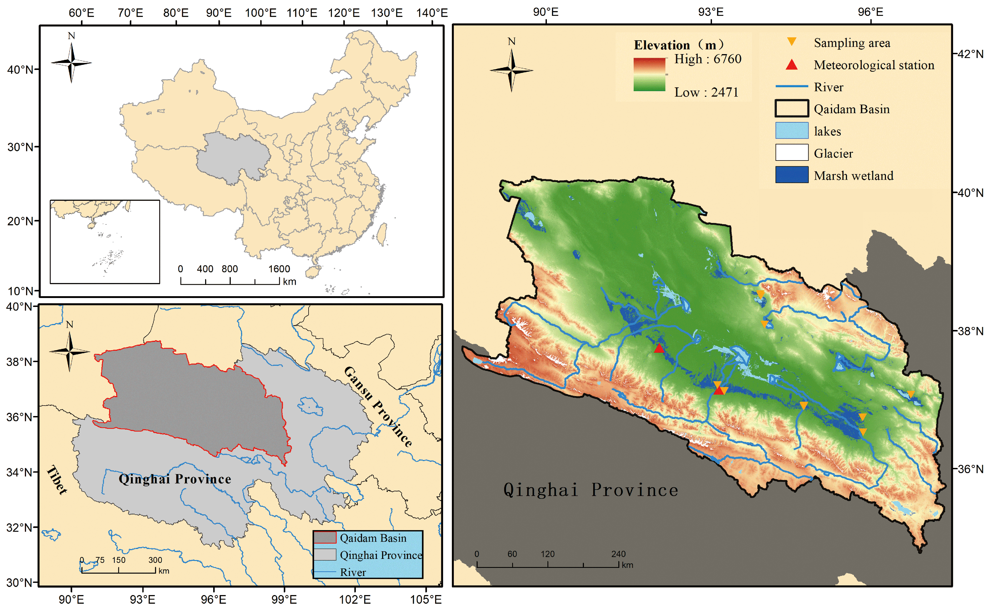
2.1. Study Area Overview

The Qaidam Basin is situated in the northeastern corner of the Qinghai–Tibet Plateau, spanning latitudes of 35°00′ to 39°20′ N and longitudes of 90°16′ to 99°16′ E (Figure 1). Encompassing an approximate area of 250,000 km², the basin’s elevation ranges from 2654 to 6588 m. Enclosed by the Kunlun Mountains, Qilian Mountains, and Altun Mountains, the Qaidam Basin takes the form of an enclosed intermountain depression that is surrounded on all sides [43]. The distribution of surface water resources within the basin is significantly influenced by topography and recent tectonic activities, exhibiting a radial pattern converging towards the center. Rivers, streams, lakes, and catchment basins provide geological conditions conducive to the development of wetlands in the region [44].

The climate of the Qaidam Basin is characterized by cold and arid conditions, with limited precipitation, strong winds, extended period of sunshine, intense solar radiation, and favorable light quality. The average annual temperature is 4.1 °C, and the average annual precipitation is 93.7 mm. In recent 30 years, both temperature and precipitation have shown an obvious rising trend [45]. The average wind speed is high, leading to numerous windy days, reflecting the distinctive features of a continental desert climate and a highland climate [46]. Lakes, marsh wetlands, and grasslands in the basin are mainly distributed in lower flat areas with lower elevations. Glacier meltwater from the mountains serves as a water source for the basin’s water systems and nurtures the marsh wetlands and grasslands in the region [38].

2.2. Data Sources

2.2.1. Landsat Surface Reflectance Data

The Landsat series of satellites is the longest-running Earth observation satellite system in the world. It has a long-term Earth observation capability with a 16-day repeat cycle. As a result, it is widely used in fields such as land surface process simulation, ecological and environmental system monitoring, and climate change analysis. Since 1987, Landsat satellites have been producing images with a resolution of 30 m, and the generation of 30 m resolution images has continued to the present day. In this study, Landsat 5/7/8 TM/ETM+/OLI Level-2 images were selected as the data source. Remote sensing images covering the study area have row numbers ranging from 33 to 36 and path numbers ranging from 133 to 139. A total of 2667 remote sensing images were used from 1 June 1990 to 1 September 2020, with a cloud cover of less than 40% (https://developers.google.com/earth-engine/datasets/catalog/landsat, accessed on 1 February 2023).

2.2.2. Soil Data

Soil, as the Earth’s surface substrate, is an auxiliary variable in distinguishing land cover types and vegetation growth conditions due to its characteristics, such as its texture and moisture content [47]. It serves as a vital data source for fine-scale land cover classification. In this study, soil texture data (250 m), soil carbon content data (250 m), soil pH data (250 m), and soil moisture data (250 m) produced by OpenLandMap were employed (https://developers.google.com/earth-engine/datasets/catalog/OpenLandMap_SOL_SOL_TEXTURE-CLASS_USDA-TT_M_v02, accessed on 1 February 2023).

2.2.3. DEM (Digital Elevation Model) Data

Surface elevation is a direct influencing factor for the redistribution of near-surface water and heat, which in turn affects the spatial distribution characteristics of underlying surfaces. In this study, digital elevation model (DEM) data were used as auxiliary data for remote sensing image classification. The DEM data used in this research are 30 m spatial resolution surface elevation images generated by the Shuttle Radar Topography Mission (SRTM) in the year 2000 (https://developers.google.com/earth-engine/datasets/catalog/USGS_SRTMGL1_003, accessed on 1 February 2023).

2.2.4. Existing Land Cover Products

Given the large extent of the study area, which makes on-site sample collection unfeasible, the Global Land Cover Fine Classification Product (GLC_FCS30) developed by Chinese Academy of Sciences was employed [15]. This product utilizes the Global Spectral Library of Earth’s Surface Properties (GSPECLib) based on MCD43A4 and ESACCI_LC2015 to automatically extract high-confidence training samples. It employs the Google Earth Engine (GEE) platform for fine classification of 16 land cover types in the Chinese region. The product’s accuracy has been validated by third-party verification points, showing an overall accuracy of 80.7% for the primary class and 71.3% for the secondary class. Within the 30 m resolution product set, the accuracy of the Chinese regional product surpasses that of FROMGLC, GlobeLand and the CLCD [48,49,50]. In this study, the secondary land cover types of GLC_FCS30 are mapped to the primary land cover types to extract sample points based on the primary cover types.

2.2.5. Meteorological Data

The monthly precipitation data for the years 1990–2016 used in this study were obtained from measurements at 2 national meteorological stations (Geermu and Xiaozaohuo) in the Qaidam Basin, provided by the China Meteorological Data Sharing Service Platform (https://data.cma.cn/, accessed on 1 February 2023). Due to the absence of some data for several years, the Global Precipitation Climatology Centre (GPCC) dataset was used, a monthly precipitation product dataset with a spatial resolution of 0.1° (http://gpcc.dwd.de/, accessed on 1 February 2023). This dataset was assessed and used to compensate for the missing values of the observed data, enabling the collection of monthly precipitation data for the period from 1990 to 2020. For more details, see Sun et al. [51].

One the other hand, the monthly evapotranspiration data for the years 1990–2020 used in this study were obtained from the monthly climate grid dataset produced by the Climatic Research Unit (CRU) (CRU TS v4.06) at the University of East Anglia, United Kingdom (https://crudata.uea.ac.uk/cru/data/hrg/, accessed on 1 February 2023) [52]. Monthly evapotranspiration data were extracted from the CRU dataset using the latitude and longitude of the meteorological stations.

2.2.6. Data on Atmospheric and Ocean Circulation Indices

The potential relationship between large-scale climate modes affecting climates of distant areas through atmospheric circulation is referred to as teleconnection. Studies have shown that atmospheric circulation plays a significant role in the occurrence of droughts in China. This part of the study attempts to clarify the causal relationship between the occurrence of droughts and the variability in large-scale climate patterns. To this end, data on the monthly atmospheric circulation indices were used, including El Niño–Southern Oscillation (ENSO) [53], North Atlantic Oscillation (NAO) [54], Pacific Decadal Oscillation (PDO) [55], Arctic Oscillation (AO) [56], and Western Pacific Index (WP) [57], which were all obtained from the National Oceanic and Atmospheric Administration (NOAA) Earth System Research Laboratory (https://www.ncdc.noaa.gov/teleconnections/, accessed on 1 February 2023).

2.3. Data Analysis

2.3.1. Construction of Annual Long-Term Wetland Ecosystem Dataset

The construction of the annual long-term wetland datasets involves several key steps, including the subdivision of the land cover remote sensing classification system, preprocessing of remote sensing images, generation of training and validation datasets, application of classification methods, image post-processing, and accuracy assessment. The primary stage of land cover classification is conducted using the Google Earth Engine (GEE) platform with machine learning (ML) classifiers [58,59], which serves as an open platform containing earth system datasets and offering cloud computing services. One of its notable advantages is the capacity to perform pixel-level analysis on images without the necessity to download and manage data locally. For this study, Landsat 5/7/8 L2 level images on the GEE platform were utilized, employing pre-packaged cloud computing methods for image preprocessing and classification. Subsequent image post-processing and accuracy assessment were executed to extract long-term wetland datasets.

2.3.2. Subdivisions of Land Cover Remote Sensing Classification System

Based on the first-level classification standards of land cover defined by the Food and Agriculture Organization (FAO) of the United Nations and the proportions of various land cover types in the Chaidamu Basin from the 2005 global 30 m land cover fine classification product created by Zhang et al. [15] and updated using China’s land use remote sensing mapping system at national scale [60], a classification system containing 8 land cover types was defined: cropland, shrub, grassland, water body, ice/snow, bare land, impervious surface, and wetland. Furthermore, according to the “Technical Regulations for National Wetland Resources Survey and Monitoring (Trial)” issued by the Chinese State Forestry and Grassland Administration in 2008, Qaidam Basin wetlands are divided into three types: lake wetlands, glacier wetlands, and marshes, corresponding to water body, ice/snow, and marsh wetland land cover types [61].

2.3.3. Preprocessing of Landsat Satellite Images

The United States Geological Survey (USGS) has produced three types of datasets for each Landsat satellite: T1, T2, and RT, all of which are available in GEE. Among them, the L2 level surface reflectance products in the T1 dataset have undergone radiometric, atmospheric, and geometric corrections, rendering them suitable for data analysis without further preprocessing. However, Landsat satellite images can be affected by cloud cover, leading to errors in the analysis and observation of ground elements [62]. As obtaining cloud-free images for large areas and short periods is challenging, cloud cover detection and filtering are essential in multi-temporal land cover mapping [63,64]. In this study, the synthesis of cloud-free images for each year was achieved in three steps. Firstly, based on the Landsat top-of-atmosphere reflectance product, GEE provides a rudimentary cloud scoring algorithm that assigns a cloud likelihood score to each pixel based on the minimum value of multiple cloudiness empirical indicators. This value ranges between 0 and 100, with higher values indicating higher cloud coverage percentages. For this study, images from June to August with scores less than or equal to 40 were selected as the raw dataset [64]. Secondly, GEE provides the CFmask cloud mask method, which utilizes spectral characteristics and shape similarities of clouds and cloud shadows using top-of-atmosphere reflectance and brightness temperature as inputs. This method is widely used in Landsat and Sentinel satellite series and demonstrates high level of identification accuracy in high-latitude regions [65,66]. In this study, the CFmask method was employed along with bitwise operations to identify clouds and cloud shadows, followed by cloud masking. Lastly, the annual remote sensing images based on median synthesis were interpolated using a time series linear interpolation method to fill in the missing parts and create complete cloud-free images for each year.

2.3.4. Generation of Training and Validation Sample Sets

In large-scale land cover classification, the accuracy and sufficiency of samples are crucial for achieving precise land cover mapping [67]. However, acquiring samples through manual field observations requires substantial amount of time and effort. Therefore, methods that combine existing high-accuracy land cover products with historical Google Earth imagery for sample collection have been widely adopted for long-term time series land cover mapping [68]. To ensure sample accuracy, time series curves such as Normalized Difference Vegetation Index (NDVI), Enhanced Vegetation Index (EVI), Normalized Burn Ratio (NBR), etc., are often utilized. Breaks for Additive Seasonal and Trend (BFAST), Continuous Change Detection and Classification (CCDC), and Landtrendr methods are employed to remove sample points with abrupt changes in time series curves [69,70,71]. The Landtrendr algorithm extracts peak values caused by factors other than noise (clouds, snow, smoke, or shadows) for each pixel in the time series. It then identifies potential breakpoints by combining the years and spectral vegetation index values of the vertices in the time series. Subsequently, it fits trajectories using both point-to-point and regression-based connections and eliminates unreasonable breakpoints using a recovery rate threshold. Finally, the fitted time series trajectories are iteratively refitted with fewer segments to find the optimal model [72]. Landtrendr monitors with a yearly time step and allows for flexible definition of time windows for synthesizing cloud-free images, making it adaptable to a wider range of scenarios. On the other hand, the NBR index is highly sensitive to factors such as chlorophyll content in vegetation leaves, charcoal content in the soil, and moisture content, which makes it extensively used in land cover change monitoring [73]. The calculation formula is as follows:

$$NBR=\frac{{\rho }_{NIR}-{\rho }_{SWIR2}}{{\rho }_{NIR}+{\rho }_{SWIR2}},$$

(1)

In this equation, ${\rho }_{NIR}$ and ${\rho }_{SWIR2}$ represent the near-infrared and second shortwave infrared bands of Landsat TM/ETM+/OLI images, respectively.

In this study, the 1990, 1995, 2000, 2005, 2010, 2015, and 2020 GLC_FCS30 land cover datasets were used, with an overall accuracy of 88%. Stratified random sampling was employed to extract sample points based on the proportion of each land cover type. Using Google satellite historical imagery and the Landtrendr method for detecting temporal changes in land cover, unchanged sample points were selected over multiple years to ensure that each land cover class had a minimum of 200 and a maximum of 800 sample points.

2.3.5. Classification and Image Post-Processing

The RF algorithm employs the concept of decision trees and makes decisions based on the majority votes from multiple weak classification trees. This method is robust in the absence of data and the presence of multicollinearity among variables and is particularly adept at handling high-dimensional samples without requiring dimension reduction operations [74]. As it increases computational complexity, the RF algorithm significantly enhances classification accuracy, making it one of the top-performing classification algorithms [75]. In this study, the RF method was applied on the GEE platform using a combination of features from Landsat TM/ETM+/OLI, including blue, green, red, near-infrared, and first and second shortwave infrared bands, as well as calculated features such as Delta Normalized Burn Ratio, greenness, and brightness from Landsat’s multiband data. Additionally, vegetation index features, terrain features, and soil attributes including soil moisture, pH, and carbon content were incorporated.

To further ensure the reliability and accuracy of the classification results, image post-processing was conducted. First, a majority filter was applied within a 3 × 3 window to achieve image smoothing and reduce classification errors caused by noise [61]. Additionally, a pixel-based time filter method was utilized to rectify unreasonable classifications stemming from the classification method. This technique employed a window length of 3 years for temporal consistency checks. For each pixel, the classification results from the year before and after were examined. If the classification result for the detection year differed from the previous year’s result but matched the subsequent year’s result, it was deemed a change in land cover type and the detection year’s classification result was assigned to the new land cover type. Otherwise, if the detection year’s result was consistent with that of the previous year, it was retained as the new land cover type. This process facilitated temporal filtering for images from the second year to the second-to-last year [76].

2.3.6. Land Cover Mapping Accuracy Assessment

In this study, the classification results were evaluated both in terms of overall classification accuracy and accuracy specific to water bodies, ice and snow, and marsh wetlands. The overall classification accuracy and accuracy of individual categories were assessed using an error matrix to compute overall accuracy and Kappa coefficient [76]. The calculation formulas are as follows:

$$\mathrm{o}\mathrm{v}\mathrm{e}\mathrm{r}\mathrm{a}\mathrm{l}\mathrm{l} \mathrm{a}\mathrm{c}\mathrm{c}\mathrm{u}\mathrm{r}\mathrm{a}\mathrm{c}\mathrm{y} (\mathrm{O}\mathrm{A})=\frac{\sum _{i=1}^8{x}_{ii}}{n^2}\times 100\%,$$

(2)

$$Kappa=\frac{p_0-p_e}{1-p_e},$$

(3)

where $x_{ii}$ represents the number of correct samples for land cover category i, n is the total number of samples in the study area, $p_0$ is the accuracy of the prediction, and $p_e$ represents accidental consistency.

2.3.7. The Standardized Precipitation Evapotranspiration Index (SPEI)

The SPEI is a widely used climate index that combines information on both precipitation and evapotranspiration to assess drought conditions. It was developed by Vicente-Serrano et al. [77]. SPEI provides a standardized index of water deficits that can be compared across different regions and climate patterns and within different time periods. It takes into account the balance between water supply (precipitation) and atmosphere water demand (evapotranspiration), considering the influence of temperature on the latter. By calculating the deviation of the actual water balance from the long-term average, SPEI quantifies the severity and duration of drought events [51]. It has been proven to be a valuable tool for monitoring and managing water resources, assessing agricultural productivity, and understanding the impacts of climate change on water and carbon availability [78,79]. The SPEI is widely used in scientific research, water management, and policymaking to support decision-making processes regarding drought mitigation and adaptation strategies [80,81].

First SPEI calculates the climatic water balance as follows:

$$D_i=P_i-{PET}_i$$

(4)

where $D_i$ represents the climatic water balance, $P_i$ is the monthly precipitation in millimeters, and PETi is the monthly potential evapotranspiration in millimeters.

The ensemble of D_i at different time scales can be represented as follows:

$$D_n^y={\sum }_{i=0}^{y-1}\left(P_{n-i}-{PET}_{n-i}\right), n\ge y$$

(5)

where $y$ represents the monthly scale, which sums up the monthly $D_i$ values with different time scales. In our study, four time scales (SPEI3, SPEI6, SPEI9, and SPEI12) were selected to detect how SPEI affects wetland ecosystem dynamics. n is the number of calculations (data size). Finally, a three-parameter log-logistic probability distribution function is used to normalize the $D_i$ data sequence and is expressed as follows:

$$F_{\left(X\right)}={\left[1+{\left(\frac{\alpha }{x-\gamma }\right)}^{\beta }\right]}^{-1}$$

(6)

where the parameters of probability distribution function (i.e., $\alpha$, $\beta$, and $\gamma$) can be calculated using L-moments method [82]. The last step is standardizing the values by converting them into a standardized normal distribution, which allows for comparison across different time scales and locations. Finally, the standardized values obtained in the previous step represent the SPEI for the selected time scale and location. Positive values indicate wetter conditions, while negative values indicate drier conditions (

Table 1. Drought classes according to Vicente-Serrano’s scheme [77].

SPEI	Drought Type
>0	No obvious drought
0 to −0.5	Mild drought
−0.5 to −1	Moderate drought
−1 to −1.5	Severe drought
−1.5 to −2	Extreme drought
<−2	Exceptional drought

), with the magnitude indicating the severity of the deviation from the long-term average. In this study, the ‘spei’ package in RStudio was utilized to analyze the SPEI. For more details, see Vicente-Serrano et al. [77].

2.3.8. Breakpoint Detection for Separating Trend and Seasonal Components (BFAST)

The BFAST method iteratively decomposes original time series data into three components: seasonal, trend, and residual, detecting and characterizing data trends and seasonal local change patterns [83,84] as shown in Equation (7). This technique has been widely employed for long-term trend detection and breakpoint identification in time series [85], visually representing the trend and cyclic model of data changes within a specified interval with confidence intervals and breakpoint locations. In this study, the ‘bfast’ package in RStudio was utilized to analyze the trend of SPEI12, investigating the non-stationary characteristics of trend features and breakpoint features. The calculation formula is as follows:

$$Y_t=S_t+T_t+e_t(t=\mathrm{1,2},3,\cdots ,n),$$

(7)

Here, $t$ denotes the observation time. $S_t$ represents the observed value at time $t$, and $S_t$ is the seasonal component, which can be used to monitor cyclical changes in the time series on an annual scale. $T_t$ is a long-term trend component, generally used to detect gradual changes in time series data over a year, with potential discontinuities during the change process. $e_t$ is the residual component, consisting of the variability caused by observational methods and atmospheric conditions, that is, the change component other than the trend and seasonal components. Given the long-time scale of the SPEI12, this paper only employs the BFAST method to detect the trend component features of SPEI12, without discussing the seasonal or cyclical component features.

2.3.9. Cross-Wavelet Transform (CWT)

To conduct teleconnected analysis of SPEI12 and atmospheric circulation indices (ENSO, NAO, PDO, AO, and WP), the cross-wavelet transform (CWT) was used [86]. The cross-wavelet transform of two time series X and Y is defined as follows:

$$W_n^{XY}=W_n^X·W_n^{Y\ast },$$

(8)

In the equation, $W_n^{XY}$ is the cross-wavelet coefficient matrix of time series $X_n$ and $Y_n$; $W_n^X$ is the wavelet coefficient matrix of time series $X_n$; $\ast$ denotes complex conjugate; $W_n^Y$ is the wavelet coefficient matrix of time series; and $W_n^{Y\ast }$ is the complex conjugate matrix. For the cross-wavelet transform power $W_n^{XY}$, the larger the power, the more significant the correlation.

3. Results

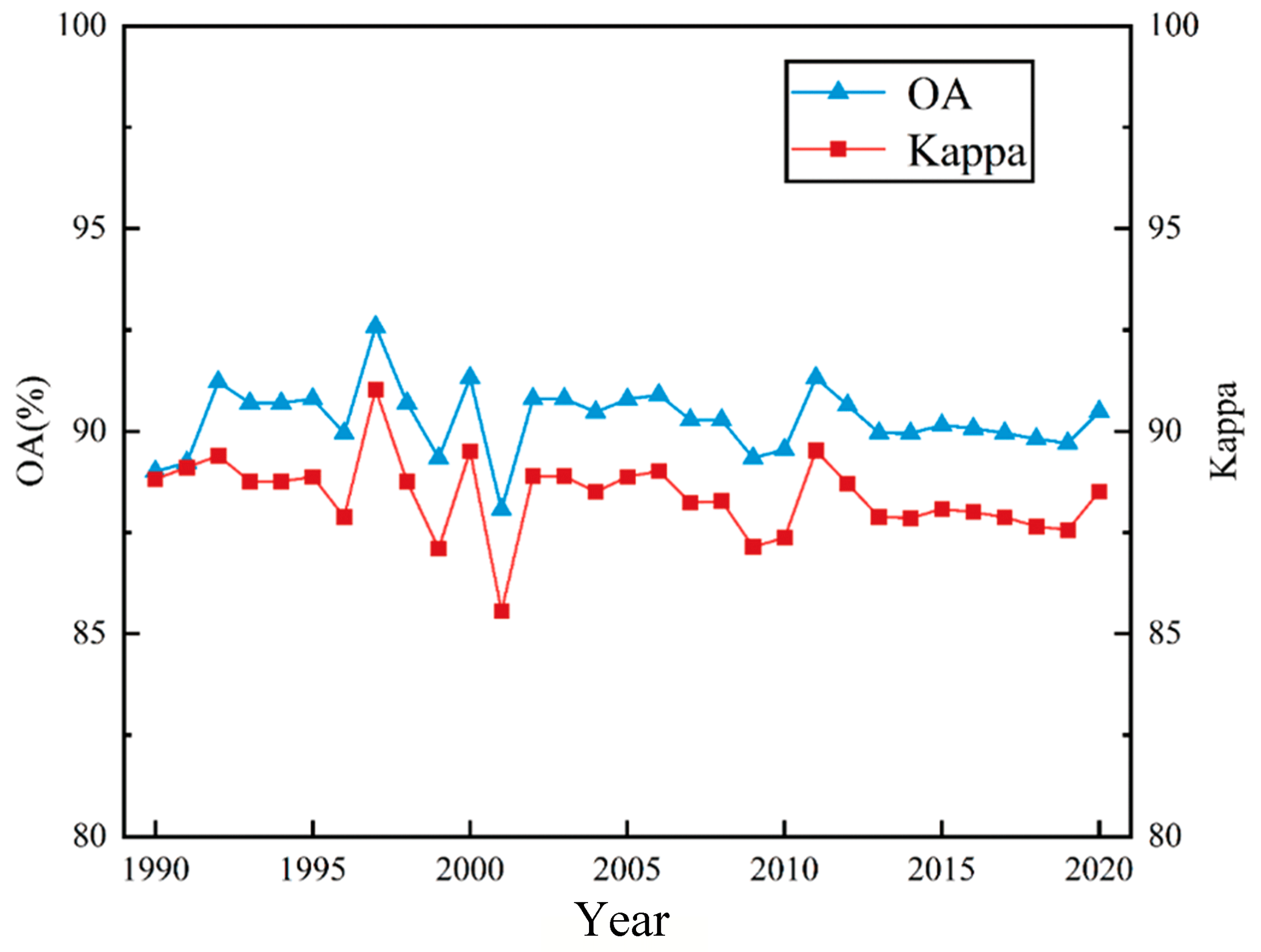
3.1. Accuracy of Wetland Extraction and Classification

As shown in Figure 2, the overall accuracy (OA) and Kappa coefficient (Kappa) exhibit a relatively stable trend over time. The multi-year average OA is 90.27%, and the multi-year average Kappa coefficient is 88.34%. The OA and Kappa coefficient experienced significant fluctuations from 1996 to 2002, with the OA ranging from 88% to 92% and the Kappa coefficient ranging from 85% to 91%. This indicates that the accuracy of the annual long time series wetland remote sensing classification dataset is relatively high, meeting the requirements for land cover change analysis.

Figure 3 depicts a land cover classification map for the Chaidamu Basin for the years 1990, 1995, 2000, 2005, 2010, 2015, and 2020. The average areas and maximum proportions of each land cover type from 1990 to 2020 are as follows: bare land (135,080 km², 56%), followed by the smallest category, built-up land (123 km², 0.05%). The average areas and proportions of other land cover types are as follows: cropland (516 km², 0.2%), shrubland (13,563 km², 6%), grassland (74,982 km², 31%), water bodies (4052 km², 2%), ice and snow (1746 km², 0.7‰), and marsh wetland (8641 km², 4%). In terms of spatial distribution, cropland and built-up land are closely related and are distributed in the low-lying areas of the basin. They tend to be located in transition zones between marshes or bare land and grassland. Shrubland and grassland are intermittently distributed in the higher-altitude areas of the basin. They are found in the Qilian Mountains to the north, the Kunlun Mountains to the southwest, and the Burhanbuda Mountains to the southeast. Water bodies are primarily concentrated in the central part of the basin, with some also occurring in valleys and depressions between the Kunlun Mountains and the Burhanbuda Mountains. Ice and snow are mainly located along the edges of the basin and on the peaks of the Qilian Mountains, Kunlun Mountains, and Burhanbuda Mountains. Notably, the snow line in the Qilian Mountains is lower than that in the Kunlun Mountains to the south and the Burhanbuda Mountains to the southeast. The marsh wetlands exhibit a strip-like distribution in the central part of the basin, with some scattered around lakes. In summary, the land cover types in the Chaidamu Basin show a strong spatial aggregation. Bare land and grassland are the predominant land cover types, reflecting a typical landscape pattern in the semi-arid region of Northwest China.

3.2. Spatial and Temporal Analysis of Wetland Changes in Chaidamu Basin

3.2.1. Analysis of Wetland Area Changes

Based on the wetland classification standards set by the National Forestry and Grassland Administration in 2010, the wetlands in the Chaidamu Basin are divided into river and lake wetlands, glacier wetlands, and marsh wetlands, corresponding to the land cover types of water bodies, ice and snow, and marsh wetlands. The total wetland area and wetland dynamism can effectively represent the quantity and magnitude of wetland changes. The changes in the total wetland area, river and lake wetland area, glacier wetland area, and marsh wetland area in the basin are shown in Figure 4. The average total wetland area in the Chaidamu Basin over the past 30 years is 14,439 km². Among them, the area of river and lake wetlands is 4091 km², the glacier wetland area is 1706 km², and the marsh wetland area is 8641 km², indicating that marsh wetlands are the dominant wetland type in the basin. The trend of wetland area changes in the Chaidamu Basin can be observed from the changes in the total wetland area over time. It can be roughly divided into three periods: 1990–1997 as growth period I, 1998–2007 as a fluctuation period, and 2008–2020 as growth period II. During growth period I, the wetland area increased from 12,865 km² to 13,731 km². In this period, the areas of river and lake wetlands and glacier wetlands decreased, while the marsh wetland area significantly increased from 7636 km² to 8880 km².

This suggests that the increase in wetland area during this period was primarily driven by the expansion of marsh wetlands. In the fluctuation period, the total wetland area showed a wave-like fluctuation trend, with minor changes. During this period, the area of river and lake wetlands increased from 3315.95 km² to 3887 km², and the glacier wetland area showed a less distinct change, while the marsh wetland area decreased from 8809 km² to 8454 km². This indicates that the fluctuation in total wetland area is influenced by the combined effects of river and lake wetlands and marsh wetlands. In growth period II, the wetland area showed a significant increasing trend, growing from 13,908 km² to 16,804 km². During this period, the area of river and lake wetlands increased in the years 2008–2011, with the highest value observed in 2010. Subsequently, the area of river and lake wetlands decreased, while the glacier wetland area increased significantly from 1603 km² to 2741 km², reaching its highest level of dynamism in 2019. The marsh wetland area also exhibited a noticeable increase, expanding from 8394 km² to 9424 km². This indicates that the significant changes in the total wetland area are the result of the combined influence of glacier wetlands and marsh wetlands.

Figure 5 illustrates the wetland transitions over the entire period (a) and during growth period I (b), the fluctuation period (c), and growth period II (d) within the basin using a chord diagram. In the entire period (1990–2020), the area transitioning from other types to wetlands was the largest (2287 km²), while the area transitioning from glaciers to lake wetlands was the smallest (59 km²). The total area transitioning from other types to wetlands is 6360 km², while the total area transitioning from wetlands is 2421 km². Internally, the most substantial transition is from lakes to glaciers (205 km²), while the transition between marshes and glaciers is minimal. During growth period I (1990–1997), the most significant transition is from other types to marsh wetlands (2137 km²), and the least significant transition is from lakes to glaciers (76 km²). The total area transitioning from other types to wetlands is 2645 km², and the total area transitioning from wetlands is 1779 km². Internally, the most substantial transition is from lakes to marshes (167 km²). In the fluctuation period (1998–2007), the most significant transition is from other types to marsh wetlands (1732 km²), and the least significant transition is from glaciers to lakes (74 km²). The total area transitioning from other types to wetlands is 2605 km², while the total area transitioning from wetlands is 2339 km². Internally, the most substantial transition is from lakes to marshes (204 km²). In growth period II (1998–2020), the most significant transition is from other types to marsh wetlands (2102 km²), and the least significant transition is from glaciers to lakes (25 km²). The total area transitioning from other types to wetlands is 4790 km², and the total area transitioning from wetlands is 1895 km². Internally, the most significant transition is from lakes to glaciers (215 km²). Comparing the wetland transitions during growth period I, the fluctuation period, and growth period II, it is evident that transitions to lakes and transitions to glaciers both increased, while transitions from glaciers to lakes decreased. Specifically, transitions to lakes increased by 834 km² in the fluctuation period compared to growth period I, and transitions to glaciers increased by 876 km² in growth period II compared to the fluctuation period. The least significant transition occurs from other types to marshes during the fluctuation period (1244 km²), and the transition from lakes to glaciers increases by 140 km² in growth period II compared to the fluctuation period. Overall, wetland area transitions are substantial during each period and over the entire period.

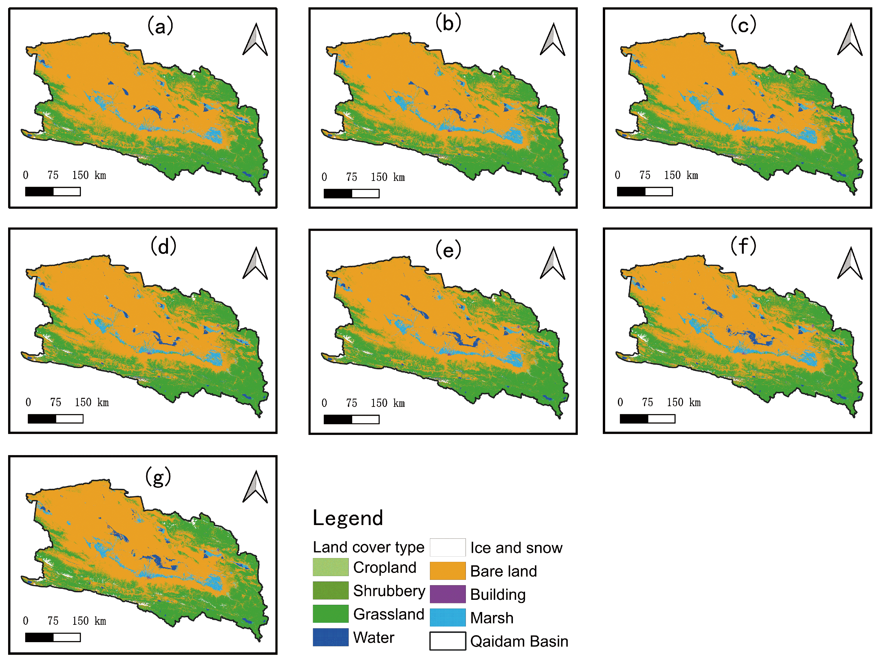
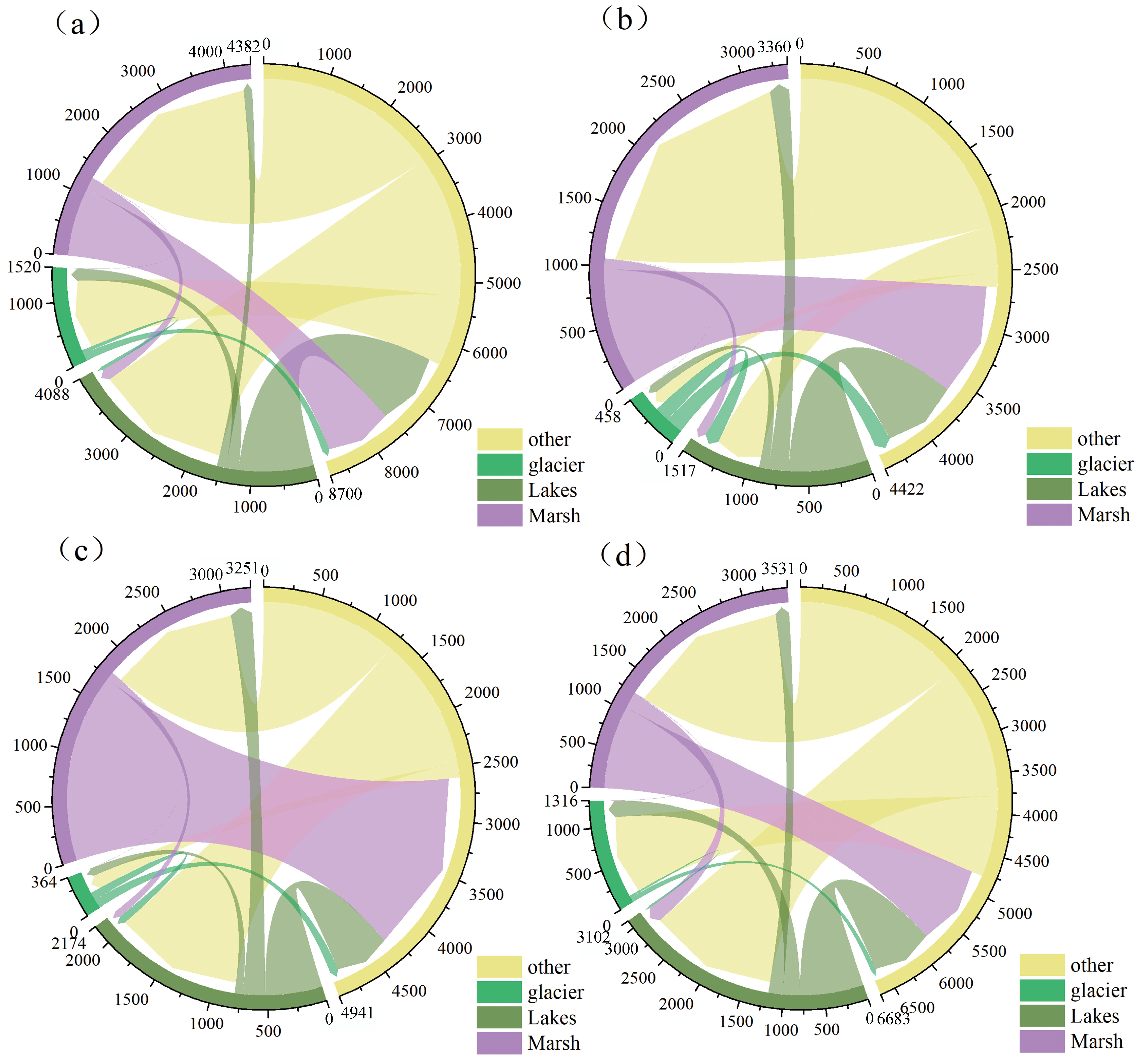
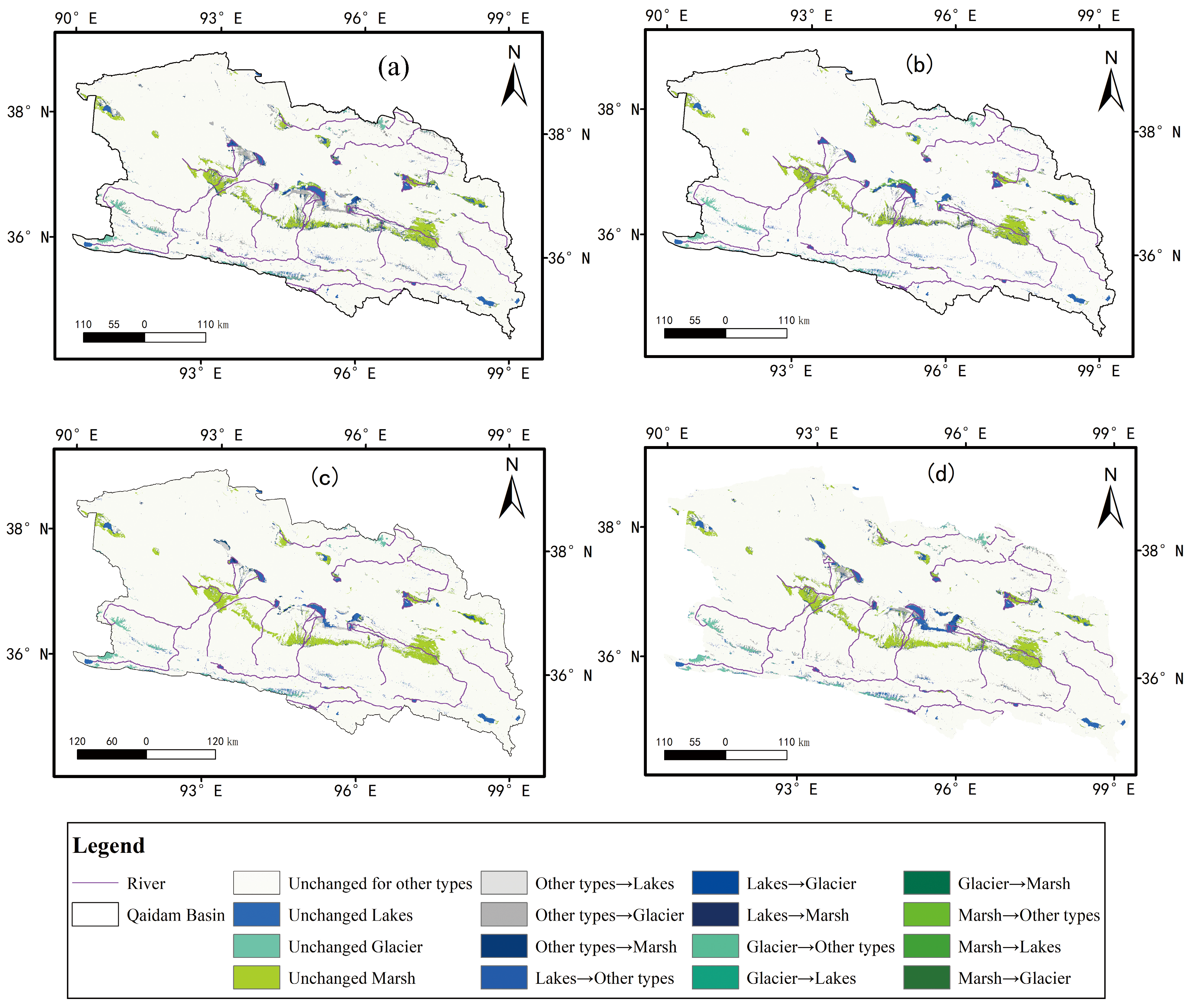
3.2.2. Analysis of Spatial Changes in Wetland Area

Based on the temporal changes in the total wetland area, the wetland area is divided into growth period I, the fluctuation period, and growth period II. As shown in Figure 6, the lake wetlands are scattered in the interior of the Qaidam Basin, the glacier wetlands exhibit a belt-like distribution in the Southern Kunlun Mountains and block-like distribution in the Northern Qilian Mountains, and the marsh wetlands are mostly concentrated in a belt-like manner from Xiangride to Wutumeiren, with a small portion scattered around the lakes in the basin. In growth period I, the spatial distribution of wetland expansion and shrinkage was different compared with the spatial change characteristics of the wetlands from 1990 to 2020, while the area of wetland expansion and shrinkage decreased. The spatial expansion of the lake wetlands was primarily concentrated in the eastern part of Qarhan Salt Lake, while the spatial shrinkage was mainly observed in the western part of East Dabson Lake and within Qarhan Salt Lake. In the shock period, compared with growth period I, the spatial distribution of wetland expansion and shrinkage was different. Lake wetland expansion was obvious for Qarhan Salt Lake, Jiner Lake, and Gasikul Lake, while the Jiner Lake wetland obviously shrank in Qarhan Salt Lake. The expansion and shrinkage of marsh wetlands have a spatial correlation in the basin. In growth phase II, compared with the shock phase, the spatial expansion of the lake wetlands was more intense in the Jinel Lake area, while the Gasikule Lake and Mahai Lake wetlands also expanded to different degrees, and the shrinkage of the North Hobson Lake wetland was obvious in the Qarhan Salt Lake area.

3.2.3. Analysis of SPEI Changes and Trends

To investigate the phenomenon of decreasing SPEIs with increasing wetland area, the BFAST method was employed to analyze the trend characteristics of SPEI12. The linear fitting result in Figure 7 shows that SPEI12 exhibits an overall decreasing trend, and this trend is statistically significant (p < 0.05), indicating a gradual shift towards drier meteorological conditions in the Qaidam Basin. The trend component in Figure 7 reveals three breakpoints in the SPEI12 time series, occurring in June 1996, May 2002, and April 2011, indicating pronounced non-stationarity in the SPEI12 time series of the Qaidam Basin. As observed from Figure 7, SPEI12 showed a decreasing trend from 1990 to 1996, followed by a sudden increase in 1996. Subsequently, from 1996 to 2002, it exhibited another decreasing trend, shifting from a relatively wet period to a relatively dry one. In 2002, it increased abruptly, indicating a shift back to a relatively wet phase. Thereafter, the trend remained stable with no evident increase. However, in 2011, SPEI12 dropped to its lowest value and subsequently remained stable without any clear increasing trend. This indicates that the Qaidam Basin experienced extreme drought conditions from 2011 to 2020. While there are some differences between these findings and the wetland evolution trend depicted in Figure 2, there are many similarities as well. During wetland growth period I, despite the decreasing trend in SPEI12, the region remained in a relatively wet phase. In the oscillation period, SPEI12 shifted from wet to dry conditions from 1996 to 2002 and then back to wet conditions from 2002 to 2007. During this period, the total wetland area also exhibited fluctuations. In growth period II, the wetland area continued to increase, but a sudden change occurred in 2012, when the area of lake wetlands began to decline. Conversely, the marsh wetlands and glacier wetlands continued to expand during this period. This discrepancy might be attributed to the drought resistance of vegetation in the marsh wetlands and the higher altitude of the glacier wetlands, which results in more complex atmospheric circulation patterns and the limited coverage of meteorological stations.

3.2.4. Effects of SPEI on Wetland Dynamics

To further investigate the factors influencing wetland changes in the Qaidam Basin, we analyzed the monthly effects of the SPEI from 1990 to 2020 on the wetland area dynamics. Correlation coefficients between the annual wetland area and SPEI at multiple time scales were calculated to assess the lagging response of wetland changes to the SPEI. The average correlation coefficient from January to December revealed a significant lag for wetland ecosystem types. As shown in Figure 8a–d, the total wetland area and different wetland types exhibited a negative correlation with the SPEI across various months and time scales, with correlation coefficients ranging from −0.791 (p < 0.01) to −0.305 (p > 0.01). Moreover, 98% of the months passed the significance test at a 0.01 level, while 2% passed at a 0.1 level. The effects of the SPEI varied across different months and time scales, persisting until the end of the year. Specifically, the lag of the SPEI at the 6-month and 12-month time scales demonstrated a delayed effect on the wetland area dynamics until August and December, respectively. Among these, SPEI12 exhibited the highest negative correlations with the wetland area dynamics. As depicted in Figure 8a–d, river and lake ecosystems showed the highest negative correlation with SPEI12, with lagged effects extending until the last four months of the year. This suggests that as SPEI12 decreased, the cumulative area of rivers and lakes increased, with correlation coefficients below −0.75 (p < 0.01) between September and December. Notably, the slow melting of mountainous glaciers during the summer and fall seasons, linked to rising temperatures during the drought events, contributes to variations in the wetland dynamics.

Additionally, the effects of SPEI12 on marsh and glacier wetlands (Figure 8c,d) were consistent with other wetland types but displayed lower responses, with correlation coefficient of −0.62 (p < 0.01) and −0.55 (p < 0.01)for the glacier and marsh wetlands, respectively. Notably, Figure 9 indicates that the river and lake areas are more influenced by the SPEI variability compared to the marsh wetlands. Interestingly, during the 2011–2012 drought event, the wetland ecosystem areas increased in the basin by approximately 13.5%, 43%, and 3.5% in the total area, the river and lake wetlands, and the glacier wetlands, respectively. This indicates the warming effects on the study area, which contributes to the melting of glacier masses, irrespective of precipitation amounts during the same drought years.

3.2.5. Response of SPEI12 to Atmospheric Circulation

Numerous research findings have demonstrated that variations in large-scale circulation patterns have a significant impact on the changes in temperature and precipitation in Northern China, consequently affecting land surface processes. Therefore, this study employs cross-wavelet transform (XWT) method to conduct a teleconnection analysis between SPEI12 and atmospheric circulation indices (ENSO, NAO, PDO, AO, WP), aiming to further elucidate the factors influencing the changes in the wetlands of the Qaidam Basin. The results are presented in Figure 10.

SPEI12 and ENSO exhibit significant positive in-phase resonance relationships with 1–2-month and 1–3-month periods in May 1993–August 1993 and January 1998–November 1998, respectively. SPEI12 and NAO show negative in-phase resonance relationships with 2–3-month and 4–5-month periods in February 1995–August 1995, August 2009–August 2014, and November 2018–October 2019. They also exhibit positive in-phase resonance relationships with 2–3-month and 2–4-month periods in August 1998–March 1999, April 2005–November 2006, and December 2016–July 2017. SPEI12 and PDO display positive in-phase resonance relationships with 2–3-month periods in October 1990–June 1991, May 2000–September 2001, and July 2012–July 2013. SPEI12 and AO demonstrate positive in-phase resonance relationships with 2–4-month and 2–3-month periods in January 2005–August 2006 and July 2008–July 2012. They also exhibit negative in-phase resonance relationships with 4–5-month, 2–4-month, and 2–3-month periods in June 2007–October 2013, February 2014–July 2016, and July 2018–April 2019. SPEI12 and WP reveal negative in-phase resonance relationships with 4–6-month, 3–4-month, and 2–3-month periods in October 1998–July 2004, January 2000–September 2001, October 2002–January 2004, and January 2010–May 2011. All of the atmospheric circulation indices mentioned above demonstrate strong correlations with SPEI12. However, in terms of resonance periods and significance levels, NAO, PDO, AO, and WP exhibit more pronounced responses to SPEI12, particularly during the 2010–2011 drought event.

4. Discussion

4.1. Land Cover Classification Results

This study utilized Landsat satellite data on the Google Earth Engine platform to classify the land cover types in the Chaidamu Basin using the RF method. The land cover types were divided into eight primary categories: cropland (516 km²), shrubland (13,563 km²), grassland (74,982 km²), water bodies (4052 km²), snow and ice (1746 km²), and marsh wetlands (8641 km²). The classification results differed from the 30 m resolution land cover dataset, particularly in the categories of marsh wetlands, snow and ice, cropland, and grassland compared to Globelandcover30. These differences can be attributed to two main factors. Firstly, the selection of samples played a role. This study utilized the 30 m resolution land cover product GLC_FCS30 [15] as the original sample data, combined with the specific Google Earth imagery features of land cover types in the Chaidamu Basin. This approach allowed for precise sample selection. While global and national land cover products use numerous samples, the quantity within small-scale regions can be limited, leading to reduced levels of sample diversity within specific regions. This can result in overfitting phenomena, in which the global fitting is good but the local fitting is poor, ultimately leading to unsatisfactory classification results in certain areas. Secondly, differences in methods and processing workflows also had an effect. Gong [49] pointed out that even for the same area, using different classification methods and processing workflows can result in variations in pixel-level land cover types, despite achieving a high level of classification accuracy. The data processing, classification, and post-processing workflows employed in this study differed from those used by previous researchers. As a result, differences in land cover types at the pixel level were inevitable due to the distinct approaches used in the methods and processes of this study.

Despite fluctuations in the total wetland area during the oscillation period, the overall trend shows a significant increase, with lake wetlands, glacier wetlands, and marsh wetlands all displaying an upward trend. This contrasts with the conclusion reached by another study on the gradual degradation of glacier wetlands in the Chaidamu Basin from 1987 to 2013 [87], and the findings by Zhang et al. [88], which indicated a decrease in glacier area in the Chaidamu Basin from 2000 to 2020. Conversely, Fan et al. [89] proposed that most glaciers on the Qinghai–Tibet Plateau have been advancing or stable over the past 50 years. Their analysis revealed that although the annual and summer temperatures are increasing within the plateau, winter temperatures are decreasing, and snowfall is on the rise, favoring ice accumulation. Zhang [90] also pointed out that the reduction in glacier area varies with glacier size, and larger glaciers experience a proportionally lower reduction. Given that the Qilian and Kunlun Mountain glaciers in the Chaidamu Basin are relatively large, their melting rate is lower. Qin [91] suggested that smaller glaciers are more sensitive to temperature increases compared to larger glaciers. Simultaneously, Su et al. [92] stated that since the 1980s, some glaciers in the middle and western sections of the Kunlun Mountains and Qilian Mountains are still advancing or are stable. In this study, we provide a certain physical basis for the observed trend of glacier expansion in the Chaidamu Basin over the past 30 years. Regarding lake wetlands in the Chaidamu Basin, Zhang et al. [88] found a decreasing trend in lake area from 2000 to 2020, while Du et al. [93] discovered there was an expansion in the total area of major lake wetlands from 1976 to 2017. Over the past 30 years, the climate within the basin has exhibited a trend towards warmer and wetter conditions, with rising temperatures and increased precipitation likely contributing to the expansion of lake wetland areas. As for marsh wetlands predominantly covered by vegetation, Du et al. [93] indicated a positive correlation between the total lake wetland area and total vegetation area. Increased precipitation in the basin enhances vegetation coverage, which promotes internal water retention and leads to the expansion of lake wetland areas. This expansion, in turn, supports further vegetation growth, creating a mutually reinforcing relationship between the vegetation ecosystem and lake water levels. As a result, this positive feedback loop contributes to the expansion of marsh wetland areas.

Zhang et al. [15] pointed out that even with a high level of accuracy, land cover classification results can deviate from actual land cover types due to differences in samples and production processes. In this study, errors resulting from inevitable sample selection may occur. When we applied our methods, we used parameters that were selected from previous studies as inputs, which may have inevitably led to model-fitting discrepancies, resulting in a lower classification accuracy. This could also be a contributing factor to discrepancies in wetland area and discrepancies between our results and the conclusions of previous researchers.

4.2. SPEI Trend and Its Impact on Wetland Ecosystems

The analysis of this study revealed that SPEI12 exhibits the highest average correlation coefficients with both the total wetland area and individual wetland types, displaying a significant negative relationship. This indicates that the annual variability characteristics of the SPEI at a 12-month scale have a pronounced impact on wetland responsiveness. This study concludes that SPEI12 in the Chaidamu Basin displayed a significant decreasing trend from 1990 to 2020 (p < 0.01), aligning with the findings of Zhang et al. [94] on the drought–wetness variability in the Qinghai–Tibet Plateau from 1979 to 2015 in the Chaidamu region. This suggests a prevailing tendency towards arid conditions in the Chaidamu Basin [94]. It is noteworthy that the SPEI values are influenced by temperature, precipitation, and evaporation. Existing research has shown an increasing trend in temperature and precipitation in the Chaidamu Basin over the past 30 years [95,96]. Higher temperatures significantly influence increased evaporation, and factors such as wind speed, relative humidity, and sunlight duration also contribute to evaporation, which is challenging to directly measure [97]. However, studies by Zhang et al. [98] on the continuous wetness characteristics of the Qinghai–Tibet Plateau from 1970 to 2017 revealed an upward trend in the SPEI during the growing season in the Chaidamu Basin, indicating an improvement in drought conditions. This further validates the conclusion that while SPEI12 indicates increased aridity within the basin, wetland areas are still expanding, an aspect that requires further research. Moreover, climate change is influenced by large-scale atmospheric circulation patterns. Studies suggest a teleconnection between Qinghai Plateau drought conditions and atmospheric circulation. The SPEI exhibits varying responses to ENSO, PDO, NAO, and AO, with the most pronounced response to PDO. Hence, we conducted a teleconnection analysis between SPEI12 and the ENSO, PDO, NAO, AO, and WP atmospheric circulation indices [99].

This study solely employed climate factors to conduct a correlation analysis of wetland area, yet human activities are also an indispensable factor in analyzing the increase in wetland area within the basin. Zhang et al. [6] analyzed the impact of climate change and human activities on wetland variations in the Qinghai–Tibet Plateau and found that the Chaidamu Basin harbors the highest proportion of artificial wetlands across the plateau. Additionally, since the release of the “Regional Ecological Construction and Environmental Protection Plan for the Qinghai–Tibet Plateau” by the Chinese government in 2011, the ecological environment of the Qinghai–Tibet Plateau has been influenced by artificial restoration efforts, leading to gradual improvements in ecological conditions [100]. Taken together, this indicates that human activities contribute to the increase in wetland area within the basin. However, the degree of response of the wetlands within the basin to human activities remains to be fully understood. Therefore, this aspect will be further explored in our future research.

Furthermore, this study solely utilized data from two national meteorological stations within the Chaidamu Basin to calculate the SPEI. The scarcity of station data makes it challenging to represent the entire basin’s meteorological drought conditions. This could potentially introduce bias to the correlation coefficient between SPEI12 and the wetland area, thereby making it difficult to explain the issue of increased wetland area coinciding with exacerbated drought conditions.

4.3. Atmospheric Circulation Mode’s Effects on the SPEI

This study reveals a robust resonance between changes in SPEI12 and atmospheric circulation indices in the Chaidamu Basin. This finding aligns with previous research by Fan et al. [99] who analyzed the spatiotemporal characteristics of drought in Qinghai Province and its response to atmospheric circulation. Numerous studies have also confirmed the relationship between the West Pacific Index and abnormal sea surface temperatures in the central and western Pacific regions [101]. Positive WP phases often coincide with warmer sea surface temperatures in the western Pacific, leading to higher temperatures and reduced precipitation in the Chaidamu Basin; conversely, negative WP phases correspond to lower temperatures and increased precipitation [99]. Warm ENSO phases (El Niño) typically result in higher sea surface temperatures in the eastern Pacific, potentially leading to warmer temperatures and reduced precipitation in the Chaidamu Basin during winter and spring. Cold ENSO phases (La Niña) might result in increased precipitation [102]. When the Arctic Oscillation (AO) is in a high index phase, the summer monsoon over the Qinghai–Tibet Plateau weakens [103]. Positive North Atlantic Oscillation (NAO) phases could lead to warmer winters and increased precipitation on the plateau, while negative phases have the opposite effect [104]. The positive and negative phases of the Pacific Decadal Oscillation (PDO) also influence temperature and precipitation patterns on the plateau. Positive PDO phases coincide with warmer sea surface temperatures in the western Pacific, causing the monsoon to move southward and increase precipitation in the plateau region, while negative PDO phases produce the opposite effects [105]. The changes in atmospheric circulation indices provide driving forces for the temperature and precipitation trends within the basin. For instance, the severe drought event experienced in Northwest China in 2010 was related to the ENSO event [106].

5. Conclusions

In this study, we employed Landsat TM/ETM/OLI data and the Google Earth Engine platform to conduct annual long-term land cover classification in the Chaidamu Basin using the RF method. Concurrently, we computed SPEI3, SPEI6, SPEI9, and SPEI12 based on monthly precipitation and evapotranspiration data. These SPEI values were utilized to characterize meteorological drought conditions in the basin. By using a Pearson’s correlation analysis, we established the relationship between wetland changes and the SPEI at various temporal scales. To investigate the impact of SPEI12 trends on wetlands, we employed the BFAST method to analyze the changing wet and dry periods for different time scales. Additionally, we explored the response of SPEI12 to atmospheric circulation by conducting a cross-wavelet analysis to assess the remote correlation between SPEI12 and atmospheric circulation factors. The study’s key conclusions are as follows:

(1) The annual long-term land cover dataset of the Chaidamu Basin from 1990 to 2020 is categorized into the following land cover types and areas: cultivated land (516 km², 0.2%), shrubland (13,563 km², 6%), grassland (74,982 km², 31%), water bodies (4052 km², 2%), ice and snow (1746 km², 0.7‰), marsh wetland (8641 km², 4%), bare land (135,080 km², 56%), and built-up land (123 km², 0.05%). The classification accuracy is represented by an overall accuracy (OA) of 90.27% and Kappa (K) coefficient of 88.34%, meeting the requirements for studying wetland changes in relation to climate changes.

(2) The wetland areas in the Chaidamu Basin, including the total wetland area, lake wetland area, glacier wetland area, and marsh wetland area, exhibit a clear increasing trend from 1990 to 2020. There are four periods of change: growth period I (1990–1997), the oscillation period (1998–2007), and growth period II (2008–2020), during which mutual conversions between different wetland types and between non-wetland types and wetlands are substantial. The most significant conversion is from non-wetland types to wetlands in terms of area. Spatially, the lake wetlands and marsh wetlands are distributed in the lower-latitude central basin area, while the glacier wetlands are found at higher altitudes in the Kunlun Mountains and Qilian Mountains.

(3) The SPEIs at 3-month, 6-month, 9-month, and 12-month scales are all significantly negatively correlated (p < 0.5) with both the total wetland area and wetland areas of different types. The lagging effect of SPEI12 on the wetlands is the strongest (between September and December), with a correlation coefficient of <−0.75. Analyzing the trend of SPEI12 from 1990 to 2020, a significant decreasing trend (p < 0.5) is observed overall. However, the time series exhibits noticeable non-stationary characteristics, with three breakpoints occurring in June 1996, May 2002, and April 2011. This trend suggests that the drought severity intensified during these periods.

(4) The atmospheric circulation indices (ENSO, NAO, PDO, AO, and WP) exhibit varying degrees of resonance with SPEI12. NAO, PDO, AO, and WP show longer resonance times, and their responses to SPEI12 are more pronounced.

(5) This study presents recommended measures to address ecological and environmental issues in the Chaidamu Basin. These measures encompass aspects such as public education, scientific research, monitoring, and water conservation promotion. It is anticipated that these measures will offer valuable insights for achieving regional sustainable development.

These conclusions deepen our understanding of wetland changes and meteorological drought conditions in the Chaidamu Basin, offering valuable information for future ecological and environmental management and conservation efforts. Additionally, this study serves as a reference for studies of similar regions and with similar methods.

References

1. Alsafadi, K.; Bi, S.; Bashir, B.; Mohammed, S.; Sammen, S.S.; Alsalman, A.; Kenawy, A. Assessment of carbon productivity trends and their resilience to drought disturbances in the middle east based on multi-decadal space-based datasets. Remote Sens. 2022, 14, 6237. [Google Scholar] [CrossRef]
2. Masson-Delmotte, V.; Zhai, P.; Pirani, A.; Connors, S.L.; Péan, C.; Berger, S.; Caud, N.; Chen, Y.; Goldfarb, L.; Gomis, M.I.; et al. Climate Change 2021: The Physical Science Basis. Contribution of Working Group I to the Sixth Assessment Report of the Intergovernmental Panel on Climate Change; Cambridge University Press: Cambridge, UK; New York, NY, USA, 2021; p. 2391. [Google Scholar]
3. Quan, Q.; Tian, D.S.; Luo, Y.Q.; Zhang, F.Y.; Tom, W.C.; Zhu, K.; Chen, Y.H.; Zhou, Q.P.; Niu, S.L. Water scaling of ecosystem carbon cycle feedback to climate warming. Sci. Adv. 2019, 5, eaav1131. [Google Scholar] [CrossRef] [PubMed]
4. Nielsen, D.L.; Kiya, P.; Watts, R.J.; Wilson, A.L. Empirical evidence linking increased hydrologic stability with decreased biotic diversity within wetlands. Hydrobiologia 2013, 708, 81–96. [Google Scholar] [CrossRef]
5. Kumari, R.; Shukla, S.K.; Parmar, K. Wetlands Conservation and Restoration for Ecosystem Services and Halt Biodiversity Loss: An Indian Perspective. In Restoration of Wetland Ecosystem: A Trajectory towards a Sustainable Environment; Springer: Singapore, 2020; pp. 75–85. [Google Scholar]
6. Zhang, Y.H.; Yan, J.Z.; Cheng, X. Research progress on impacts of climate change and human activities on wetlands on the Qinghai-Tibet Plateau. Acta Ecol. Sin. 2023, 43, 2180–2193. [Google Scholar]
7. Nicholls, R.J. Coastal flooding and wetland loss in the 21st century: Changes under the SRES climate and socio-economic scenarios. Glob. Environ. Chang. 2004, 14, 69–86. [Google Scholar] [CrossRef]
8. Davidson, N.C. How much wetland has the world lost? Long-term and recent trends in global wetland area. Mar. Freshw. Res. 2014, 65, 936–941. [Google Scholar] [CrossRef]
9. Zhong, Y.F.; Wu, H.; Liu, Y.H. Research status and prospect of wetland remote sensing mapping. Bull. Natl. Nat. Sci. Found. China 2022, 36, 420–431. [Google Scholar]
10. Mao, D.; Wang, Z.; Du, B.; Li, L.; Tian, Y.; Jia, M.; Zeng, Y.; Song, K.; Jiang, M.; Wang, Y. National wetland mapping in China: A new product resulting from object-based and hierarchical classification of Landsat 8 OLI images. ISPRS J. Photogramm. Remote Sens. 2020, 164, 11–25. [Google Scholar] [CrossRef]
11. Gong, P.; Niu, Z.G.; Cheng, X. China’s wetland change (1990–2000) determined by remote sensing. Sci. Sin. 2010, 40, 768–775. [Google Scholar] [CrossRef]
12. Xu, X.C.; Li, B.J.; Liu, X.P. Global annual land cover map at 30 m resolution from 2000 to 2015. Natl. Remote Sens. Bull. 2021, 25, 1896–1916. [Google Scholar]
13. Chen, J.; Chen, J.; Liao, A. Global land cover mapping at 30m resolution: A POK-based operational approach. ISPRS J. Photogramm. Remote Sens. 2015, 103, 7–27. [Google Scholar] [CrossRef]
14. Zhang, S.Y.; Hu, F. GlobeLand30 land cover products are used for refined wind energy resource assessment. Resour. Sci. 2017, 39, 125–135. [Google Scholar]
15. Zhang, X.; Liu, L.; Chen, X.; Gao, Y.; Xie, S.; Mi, J. GLC_FCS30: Global land-cover product with fine classification system at 30 m using time-series Landsat imagery. Earth Syst. Sci. Data 2021, 13, 2753–2776. [Google Scholar] [CrossRef]
16. Wang, Y.; Hu, Y.; Niu, X. Myanmar’s Land Cover Change and Its Driving Factors during 2000–2020. Int. J. Environ. Res. Public Health 2023, 20, 2409. [Google Scholar] [CrossRef] [PubMed]
17. Mousivand, A.; Arsanjani, J.J. Insights on the historical and emerging global land cover changes: The case of ESA-CCI-LC datasets. Appl. Geogr. 2019, 106, 82–92. [Google Scholar] [CrossRef]
18. Reinhart, V.; Hoffmann, P.; Rechid, D.; Böhner, J.; Bechtel, B. High-resolution land use and land cover dataset for regional climate modelling: A plant functional type map for Europe 2015. Earth Syst. Sci. Data 2022, 4, 1735–1794. [Google Scholar] [CrossRef]
19. Yang, J.; Huang, X. The 30 m annual land cover dataset and its dynamics in China from 1990 to 2019. Earth Syst. Sci. Data 2021, 13, 3907–3925. [Google Scholar] [CrossRef]
20. Sun, W.; Ding, X.; Su, J.; Mu, X.; Zhang, Y.; Gao, P.; Zhao, G. Land use and cover changes on the Loess Plateau: A comparison of six global or national land use and cover datasets. Land Use Policy 2022, 119, 106165. [Google Scholar] [CrossRef]
21. Zhang, W.J.; Shang, Z.Y.; Zhang, J.; Yan, S.; Deng, A.; Zhang, X.; Zheng, C.; Song, Z. Standardized Establishment and Improvement of Accounting System of Agriculture Greenhouse Gas Emission. Sci. Agric. Sin. 2023, 56, 4467–4477. [Google Scholar]
22. Van Lanen, H.A.; Wanders, N.; Tallaksen, L.M.; Van Loon, A.F. Hydrological drought across the world: Impact of climate and physical catchment structure. Hydrol. Earth Syst. Sci. 2013, 17, 1715–1732. [Google Scholar] [CrossRef]
23. Li, Y.J.; Ren, F.M.; Li, Y.P. Characteristics of regional meteorological drought events in Southwest China from 1960 to 2010. Acta Meteorol. Sin. 2014, 72, 266–276. [Google Scholar]
24. Zhang, J.F.; Tang, W.J.; Li, S.L. Discussion on identification of drought-prone areas in southwest China. China Water Resour. 2012, 5, 18–21+39. [Google Scholar]
25. Wang, D.; Zhang, B.; An, M.L. Spatiotemporal characteristics of drought in Southwest China during the last 53 years based on SPEI. J. Nat. Resour. 2014, 29, 1003–1016. [Google Scholar]
26. Li, Y.J.; Ding, J.L.; Zhang, Y.Y. Response of vegetation cover to drought on the north slope of Tianshan Mountains from 2001 to 2015: Based on land use/land cover analysis. Acta Ecol. Sin. 2019, 39, 6206–6217. [Google Scholar]
27. Mokhtar, A.; He, H.; Alsafadi, K. Evapotranspiration as a response to climate variability and ecosystem changes in southwest, China. Environ. Earth Sci. 2020, 79, 312. [Google Scholar] [CrossRef]
28. Chen, J.I.; Sun, H.W.; Wang, J.P. Improvement of comprehensive meteorological drought index and its applicability analysis. Trans. Chin. Soc. Agric. Eng. 2020, 36, 71–77. [Google Scholar]
29. Sobral, B.S.; De, O.J.F.; De, G.G. Drought characterization for the state of Rio de Janeiro based on the annual SPI index: Trends, statistical tests and its relation with ENSO. Atmos. Res. 2019, 220, 141–154. [Google Scholar] [CrossRef]
30. Byun, H.R.; Wilhite, D.A. Objective Quantification of Drought Severity and Duration. J. Clim. 1999, 12, 2747–2756. [Google Scholar] [CrossRef]
31. Liu, Y.; Yang, X.; Ren, L. A New Physically Based Self-Calibrating Palmer Drought Severity Index and its Performance Evaluation. Water Resour. Manag. 2015, 29, 4833–4847. [Google Scholar] [CrossRef]
32. Yang, Q.; Li, M.X.; Zheng, Y.Z. Regional adaptability of 7 meteorological drought indices in China. Sci. Sin. (Terrae) 2017, 47, 337–353. [Google Scholar]
33. Feng, D.L.; Cheng, Z.G.; Zhao, L. Applicability analysis of four drought discrimination indexes in Northeast China. Arid. Land Geogr. 2020, 43, 371–379. [Google Scholar]
34. Li, L.; She, D.; Zheng, H. Elucidating Diverse Drought Characteristics from Two Meteorological Drought Indices (SPI and SPEI) in China. J. Hydrometeorol. 2020, 21, 1513–1530. [Google Scholar] [CrossRef]
35. Xiong, G.J.; Wang, S.G.; Li, C.Y. Applicability analysis of three drought indices in southwest China. Plateau Meteorol. 2014, 33, 686–697. [Google Scholar]
36. Chen, H.; Sun, J. Changes in Drought Characteristics over China Using the Standardized Precipitation Evapotranspiration Index. J. Clim. 2015, 28, 5430–5447. [Google Scholar] [CrossRef]
37. Wang, W.; Guo, B.; Zhang, Y. The sensitivity of the SPEI to potential evapotranspiration and precipitation at multiple timescales on the Huang-Huai-Hai Plain, China. Theor. Appl. Climatol. 2020, 143, 87–99. [Google Scholar] [CrossRef]
38. Zhao, Z.; Zhang, Y.; Liu, L. Recent changes in wetlands on the Tibetan Plateau: A review. J. Geogr. Sci. 2015, 25, 879–896. [Google Scholar] [CrossRef]
39. Li, H.; Mao, D.; Li, X.; Wang, Z.; Wang, C. Monitoring 40-Year Lake Area Changes of the Qaidam Basin, Tibetan Plateau, Using Landsat Time Series. Remote Sens. 2019, 11, 343. [Google Scholar] [CrossRef]
40. Shen, X.; Liu, B.; Jiang, M.; Wang, Y.; Wang, L.; Zhang, J.; Lu, X. Spatiotemporal change of marsh vegetation and its response to climate change in China from 2000 to 2019. J. Geophys. Res. Biogeosciences 2021, 126, e2020JG006154. [Google Scholar] [CrossRef]
41. Cao, S.; Zhang, L.; He, Y. Effects and contributions of meteorological drought on agricultural drought under different climatic zones and vegetation types in Northwest China. Sci. Total Environ. 2022, 821, 153270. [Google Scholar] [CrossRef] [PubMed]
42. Bai, M.; Mo, X.; Liu, S.; Hu, S. Detection and attribution of lake water loss in the semi-arid Mongolian Plateau—A case study in the Lake Dalinor. Ecohydrology 2021, 14, e2251. [Google Scholar] [CrossRef]
43. Zhang, M.; Liu, X. Climate changes in the Qaidam Basin in NW China over the past 40 kyr. Palaeogeogr. Palaeoclimatol. Palaeoecol. 2020, 551, 109679. [Google Scholar] [CrossRef]
44. Bao, J.; Wang, Y.; Song, C.; Feng, Y.; Hu, C.; Zhong, S.; Yang, J. Cenozoic sediment flux in the Qaidam Basin, northern Tibetan Plateau, and implications with regional tectonics and climate. Glob. Planet. Chang. 2017, 155, 56–69. [Google Scholar] [CrossRef]
45. Qi, D.M.; Li, Y.Q.; Zhou, C.Y. Climate change characteristics and causes of water vapor budget over the Tibetan Plateau during 1979–2016. J. Glaciol. Geocryol. 2023, 45, 846–864. [Google Scholar]
46. Rohrmann, A.; Heermance, R.; Kapp, P.; Cai, F. Wind as the primary driver of erosion in the Qaidam Basin, China. Earth Planet. Sci. Lett. 2013, 374, 1–10. [Google Scholar] [CrossRef]
47. Hurskainen, P.; Adhikari, H.; Siljander, M.; Pellikka, P.K.E.; Hemp, A. Auxiliary datasets improve accuracy of object-based land use/land cover classification in heterogeneous savanna landscapes. Remote Sens. Environ. 2019, 233, 111354. [Google Scholar] [CrossRef]
48. Liu, J.; Ren, Y.; Chen, X. Regional Accuracy Assessment of 30-Meter GLC_FCS30, GlobeLand30, and CLCD Products: A Case Study in Xinjiang Area. Remote Sens. 2024, 16, 82. [Google Scholar] [CrossRef]
49. Gong, P.; Liu, H.; Zhang, M.; Li, C.; Wang, J.; Huang, H.; Clinton, N. Stable Classification with Limited Sample: Transferring a 30-m Resolution Sample Set Collected in 2015 to Mapping 10-m Resolution Global Land Cover in 2017. Sci. Bull. 2019, 64, 370–373. [Google Scholar] [CrossRef]
50. Wang, J.Y.; Xin, L.J. Temporal and spatial changes of cultivated land and grain production in China based on GlobeLand30 data. Trans. Chin. Soc. Agric. Eng. 2017, 33, 8. [Google Scholar]
51. Sun, J.; Bi, S.; Bashir, B.; Ge, Z.; Wu, K.; Alsalman, A.; Ayugi, B.O.; Alsafadi, K. Historical Trends and Characteristics of Meteorological Drought Based on Standardized Precipitation Index and Standardized Precipitation Evapotranspiration Index over the Past 70 Years in China (1951–2020). Sustainability 2023, 15, 10875. [Google Scholar] [CrossRef]
52. Harris, I.; Osborn, T.J.; Jones, P.; Lister, D. Version 4 of the CRU TS Monthly High-Resolution Gridded Multivariate Climate Dataset. Sci. Data 2020, 7, 109. [Google Scholar] [CrossRef]
53. Barnston, A.G.; Chelliah, M.; Goldenberg, S.B. Documentation of highly ENSO-related SST region in the equatorial Pacific. Atmosphere-Ocean 1997, 35, 367–383. [Google Scholar]
54. Hurrell, J.W. Decadal trends in the North Atlantic Oscillation: Regional temperatures and precipitation. Science 1995, 269, 676–679. [Google Scholar] [CrossRef] [PubMed]
55. Mantua, N.J.; Hare, S.R.; Zhang, Y.; Wallace, J.M.; Francis, R.C. A Pacific interdecadal climate oscillation with impacts on salmon production. Bull. Am. Meteorol. Soc. 1997, 78, 1069–1080. [Google Scholar] [CrossRef]
56. Thompson, D.W.; Wallace, J.M.; Hegerl, G.C. Annular modes in the extratropical circulation. Part II: Trends. J. Clim. 2000, 13, 1018–1036. [Google Scholar] [CrossRef]
57. Barnston, A.G.; Livezey, R.E. Classification, seasonality and persistence of low-frequency atmospheric circulation patterns. Mon. Weather. Rev. 1987, 115, 1083–1126. [Google Scholar] [CrossRef]
58. Feizizadeh, B.; Omarzadeh, D.; Kazemi Garajeh, M.; Lakes, T.; Blaschke, T. Machine learning data-driven approaches for land use/cover mapping and trend analysis using Google Earth Engine. J. Environ. Plan. Manag. 2023, 66, 665–697. [Google Scholar] [CrossRef]
59. Nasiri, V.; Deljouei, A.; Moradi, F.; Sadeghi, S.M.M.; Borz, S.A. Land Use and Land Cover Mapping Using Sentinel-2, Landsat-8 Satellite Images, and Google Earth Engine: A Comparison of Two Composition Methods. Remote Sens. 2022, 14, 1977. [Google Scholar] [CrossRef]
60. Ning, J.; Liu, J.; Kuang, W. Spatiotemporal patterns and characteristics of land-use change in China during 2010–2015. J. Geogr. Sci. 2018, 28, 547–562. [Google Scholar] [CrossRef]
61. Ding, J.L.; Ge, X.Y.; Wang, J.Z. Ebinur Lake wetland identification and its spatio-temporal dynamic changes. J. Nat. Resour. 2021, 36, 1949–1963. [Google Scholar] [CrossRef]
62. Joshi, P.P.; Wynne, R.H.; Thomas, V.A. Cloud detection algorithm using SVM with SWIR2 and tasseled cap applied to Landsat 8. Int. J. Appl. Earth Obs. Geoinf. 2019, 82, 101898. [Google Scholar] [CrossRef]
63. Brooks, E.B.; Thomas, V.A.; Wynne, R.H. Fitting the Multitemporal Curve: A Fourier Series Approach to the Missing Data Problem in Remote Sensing Analysis. IEEE Trans. Geosci. Remote Sens. 2012, 50, 3340–3353. [Google Scholar] [CrossRef]
64. Irish, R.R.; Barker, J.L.; Goward, S.N. Characterization of the Landsat-7 ETM+ Automated Cloud-Cover Assessment (ACCA) Algorithm. Photogramm. Eng. Remote Sens. 2006, 72, 1179–1188. [Google Scholar] [CrossRef]
65. Zhu, Z.; Woodcock, C.E. Object-based cloud and cloud shadow detection in Landsat imagery. Remote Sens. Environ. 2012, 118, 83–94. [Google Scholar] [CrossRef]
66. Qiu, S.; He, B.; Zhu, Z. Improving Fmask cloud and cloud shadow detection in mountainous area for Landsats 4–8 images. Remote Sens. Environ. 2017, 199, 107–119. [Google Scholar] [CrossRef]
67. Foody, G.M.; Mathur, A. Toward intelligent training of supervised image classifications: Directing training data acquisition for SVM classification. Remote Sens. Environ. 2004, 93, 107–117. [Google Scholar] [CrossRef]
68. Li, W.; Dong, R.; Fu, H.; Wang, J.; Yu, L.; Gong, P. Integrating Google Earth imagery with Landsat data to improve 30-m resolution land cover mapping. Remote Sens. Environ. 2020, 237, 111563. [Google Scholar] [CrossRef]
69. Huang, Y.B.; Liao, S.B. Automatic extraction of land cover samples from multi-source data. Natl. Remote Sens. Bull. 2017, 21, 757–766. [Google Scholar] [CrossRef]
70. Verbesselt, J.; Zeileis, A.; Herold, M. Near real-time disturbance detection using satellite image time series. Remote Sens. Environ. 2012, 123, 98–108. [Google Scholar] [CrossRef]
71. Zhu, Z.; Woodcock, C.E. Continuous Change Detection and Classification of Land Cover Using All Available Landsat Data. Remote Sens. Environ. 2013, 144, 152–171. [Google Scholar] [CrossRef]
72. Kennedy, R.E.; Yang, Z.; Cohen, W.B. Detecting trends in forest disturbance and recovery using yearly Landsat time series: 1. LandTrendr—Temporal segmentation algorithms. Remote Sens. Environ. 2010, 114, 2897–2910. [Google Scholar] [CrossRef]
73. Schneibel, A.; Stellmes, M.; Röder, A.; Frantz, D.; Kowalski, B.; Haß, E.; Hill, J. Assessment of spatio-temporal changes of smallholder cultivation patterns in the Angolan Miombo belt using segmentation of Landsat time series. Remote Sens. Environ. 2017, 195, 118–129. [Google Scholar] [CrossRef]
74. Rodriguez-Galiano, V.F.; Ghimire, B.; Rogan, J.; Chica-Olmo, M.; Rigol-Sanchez, J.P. An assessment of the effectiveness of a random forest classifier for land-cover classification. ISPRS J. Photogramm. Remote Sens. 2012, 67, 93–104. [Google Scholar] [CrossRef]
75. Dai, X.Q.; Shen, R.Q.; Wang, J. Land use change detection in Henan Province supported by GEE remote sensing cloud platform. J. Geomat. Sci. Technol. 2021, 38, 287–294. [Google Scholar]
76. Zhang, M.; Li, G.; He, T. Reveal the severe spatial and temporal patterns of abandoned cropland in China over the past 30 years. Sci. Total Environ. 2023, 857, 159591. [Google Scholar] [CrossRef]
77. Vicente-Serrano, S.M.; Beguería, S.; López-Moreno, J.I. A Multiscalar Drought Index Sensitive to Global Warming: The Standardized Precipitation Evapotranspiration Index. J. Clim. 2010, 23, 1696–1718. [Google Scholar] [CrossRef]
78. Alsafadi, K.; Bashir, B.; Mohammed, S.; Abdo, H.G.; Mokhtar, A.; Alsalman, A.; Cao, W. Response of Ecosystem Carbon–Water Fluxes to Extreme Drought in West Asia. Remote Sens. 2024, 16, 1179. [Google Scholar] [CrossRef]
79. Alsafadi, K.; Al-Ansari, N.; Mokhtar, A.; Mohammed, S.; Elbeltagi, A.; Sammen, S.S.; Bi, S. An evapotranspiration deficit-based drought index to detect variability of terrestrial carbon productivity in the Middle East. Environ. Res. Lett. 2022, 17, 014051. [Google Scholar] [CrossRef]
80. Alsafadi, K.; Mohammed, S.A.; Ayugi, B.; Sharaf, M.; Harsányi, E. Spatial–temporal evolution of drought characteristics over Hungary between 1961 and 2010. Pure Appl. Geophys. 2020, 177, 3961–3978. [Google Scholar] [CrossRef]
81. Mokhtar, A.; Jalali, M.; He, H.; Al-Ansari, N.; Elbeltagi, A.; Alsafadi, K.; Abdo, H.G.; Sammen, S.S.; Gyasi-Agyei, Y.; Rodri-go-Comino, J. Estimation of SPEI Meteorological Drought Using Machine Learning Algorithms. IEEE Access 2021, 9, 65503–65523. [Google Scholar] [CrossRef]
82. Ahmad, M.I.; Sinclair, C.D.; Werritty, A. Log-logistic flood frequency analysis. J. Hydrol. 1988, 98, 205–224. [Google Scholar] [CrossRef]
83. Verbesselt, J.; Hyndman, R.; Zeileis, A.; Culvenor, D. Phenological change detection while accounting for abrupt and gradual trends in satellite image time series. Remote Sens. Environ. 2010, 114, 2970–2980. [Google Scholar] [CrossRef]
84. Verbesselt, J.; Hyndman, R.; Newnham, G.; Culvenor, D. Detecting trend and seasonal changes in satellite image time series. Remote Sens. Environ. 2010, 114, 106–115. [Google Scholar] [CrossRef]
85. Mendes, M.P.; Rodriguez-Galiano, V.; Aragones, D. Evaluating the BFAST method to detect and characterise changing trends in water time series: A case study on the impact of droughts on the Mediterranean climate. Sci. Total Environ. 2022, 846, 157428. [Google Scholar] [CrossRef] [PubMed]
86. Cazelles, B.; Chavez, M.; Berteaux, D.; Ménard, F.; Vik, J.O.; Jenouvrier, S.; Stenseth, N.C. Wavelet analysis of ecological time series. Oecologia 2008, 156, 287–304. [Google Scholar] [CrossRef]
87. Wang, Z.; Li, X.Q.; Liu, L.X. Evolution analysis of ice and snow lakes in Qaidam Basin based on remote sensing and GIS. Yangtze River 2015, 46, 64–66+91. [Google Scholar]
88. Zhang, C.; Yao, X.J.; Xiao, J.S. Evolution of glaciers and lakes in Qinghai Province from 2000 to 2020. J. Nat. Resour. 2023, 38, 822–838. [Google Scholar]
89. Fan, Q.S.; Shao, Z.J.; Cao, G.C. Impact assessment of climate change on glacier resources in Qinghai Plateau. J. Arid. Land Resour. Environ. 2005, 5, 56–60. [Google Scholar]
90. Zhang, X.S. Recent glacier retreat, climate change and sea level rise. Adv. Earth Sci. 1989, 3, 61–66. [Google Scholar]
91. Qin, D.H. Glaciers and Ecological Environment on the Qinghai-Tibet Plateau; China Tibetology Publishing House: Beijing, China, 1999. [Google Scholar]
92. Su, Z.; Liu, Z.X.; Wang, W. Response and trend prediction of glaciers on the Qinghai-Tibet Plateau to climate change. Adv. Earth Sci. 1999, 6, 607–612. [Google Scholar]
93. Du, Y.; Liu, B.K.; He, W.G. Changes of lake area and its causes in Qaidam Basin from 1976 to 2017. J. Glaciol. Geocryol. 2018, 40, 1275–1284. [Google Scholar]
94. Zhang, L.; Gao, L.; Coscarelli, R. Drought and Wetness Variability and the Respective Contribution of Temperature and Precipitation in the Qinghai-Tibetan Plateau. Adv. Meteorol. 2021, 2021, 7378196. [Google Scholar] [CrossRef]
95. Wang, X.J.; Yang, M.X.; Liang, X.W. The dramatic climate warming in the Qaidam Basin, northeastern Tibetan Plateau, during 1961–2010. Int. J. Climatol. 2014, 34, 1524–1537. [Google Scholar] [CrossRef]
96. Yang, X.W.; Wang, N.L.; Chen, A.A. Impacts of Climate Change, Glacier Mass Loss and Human Activities on Spatiotemporal Variations in Terrestrial Water Storage of the Qaidam Basin, China. Remote Sens. 2022, 14, 2186. [Google Scholar] [CrossRef]
97. Wang, H.J.; Chen, Y.N.; Pan, Y.P. Assessment of candidate distributions for SPI/SPEI and sensitivity of drought to climatic variables in China. Int. J. Climatol. 2019, 39, 4392–4412. [Google Scholar] [CrossRef]
98. Zhang, H.; Ding, M.; Li, L. Continuous Wetting on the Tibetan Plateau during 1970–2017. Water 2019, 11, 2605. [Google Scholar] [CrossRef]
99. Fan, L.; Lv, A.H.; Zhang, W.X. Temporal and spatial characteristics of drought in Qinghai Province and its response to atmospheric circulation. J. Arid. Land Resour. Environ. 2021, 35, 60–65. [Google Scholar]
100. Lin, Z.Y.; Xiao, Y.; Ou-yang, Z.Y. Assessment of ecological importance of the Qinghai-Tibet Plateau based on ecosystem service flows. J. Mt. Sci. 2021, 18, 1725–1736. [Google Scholar] [CrossRef]
101. Qian, D.L.; Guan, Z.Y.; Xu, J.Y. Prediction models for summertime Western Pacific Subtropical High based on the leading SSTA modes in the tropical Indo-Pacific sector. Trans. Atmos. Sci. 2021, 44, 405–417. [Google Scholar]
102. Li, Y.; Hou, Z.; Zhang, L.; Song, C.; Piao, S.; Lin, J.; Peng, S.; Fang, K.; Yang, J.; Qu, Y.; et al. Rapid expansion of wetlands on the Central Tibetan Plateau by global warming and El Niño. Sci. Bull. 2023, 68, 485–488. [Google Scholar] [CrossRef] [PubMed]
103. Lv, C.Y.; Liu, M.X.; Li, Y. Characteristics of summer extreme heavy precipitation in the Qaidam Basin and causes of atmospheric circulation. J. Lanzhou Univ. (Nat. Sci.) 2021, 57, 252–262. [Google Scholar]
104. Liu, S.S.; Zhou, S.W.; Wu, P. Response of winter precipitation in eastern Tibetan Plateau to Arctic Oscillation. Acta Meteorol. Sin. 2021, 79, 558–569. [Google Scholar]
105. Xie, C.X. Effect of North Atlantic Oscillation on water vapor transport over the Tibetan Plateau in winter. J. Meteorol. Res. Appl. 2023, 44, 78–84. [Google Scholar]
106. Zhang, L.; Wang, B.F.; Xin, M.Y. Atmospheric Circulation Analysis of Persistent Drought in Eastern Part of Northwest China. J. Anhui Agric. Sci. 2017, 45, 196–198. [Google Scholar]
Figure 1. The study area.
Sustainability 16 04738 g001
Figure 2. Land cover classification accuracy.
Sustainability 16 04738 g002
Figure 3. (ag) depict the land cover of the Chaidamu Basin for the years 1990, 1995, 2000, 2005, 2010, 2015, and 2020, respectively.
Sustainability 16 04738 g003
Figure 4. The area (km2) of (a) wetlands, (b) river and lake wetlands, (c) glacier wetlands, and (d) marsh wetlands within the basin.
Sustainability 16 04738 g004
Figure 5. Represents the mutual transformation (km2) of three wetland types at each stage, including (a) 1990–2020, (b) 1990–1997, (c) 1998–2007, and (d) 2008–2020.
Sustainability 16 04738 g005
Figure 6. The spatial distribution of wetland mutual transitions within the Qaidam Basin, including (a) 1990–2020, (b) 1990–1997, (c) 1998–2007, and (d) 2008–2020.
Sustainability 16 04738 g006
Figure 7. The overall trend of SPEI12 from 1990 to 2020, and the segmented trend analysis results of SPEI12 using the BFAST method from 1990 to 2020. Y t denotes the observation of SPEI12, S t is the seasonal component, T t is the long-term trend component, and e t is the residual component.
Sustainability 16 04738 g007
Figure 8. The relationship between wetland area and SPEI3, SPEI6, SPEI9, and SPEI12 from 1990 to 2020, including (a) wetlands, (b) river and lake wetlands, (c) glacier wetlands, and (d) marsh wetlands within the basin.
Sustainability 16 04738 g008
Figure 9. Statistical values of correlation coefficients between wetland area and SPEI, including (a) wetlands, (b) river and lake wetlands, (c) glacier wetlands, and (d) marsh wetlands within the basin.
Sustainability 16 04738 g009
Figure 10. SPEI12’s response to atmospheric circulation, including (a) ENSO-SPEI, (b) NAO-SPEI, (c) PDO-SPEI, (d) AO-SPEI, and (e) WP-SPEI.
Sustainability 16 04738 g010