Article

High-Profile Convoy Disruptions: Exploring Socioeconomic and Environmental Ramifications of Road Closures

1
School of Civil & Environmental Engineering, College of Engineering, King Faisal University, Al Hofuf 31982, Saudi Arabia
2
School of Civil & Environmental Engineering (SCEE), National University of Sciences and Technology (NUST), Islamabad 44000, Pakistan
3
Department of Civil, Construction and Environmental Engineering, North Dakota State University, Fargo, ND 58102, USA
*
Author to whom correspondence should be addressed.
Sustainability 2024, 16(13), 5278; https://doi.org/10.3390/su16135278
Submission received: 25 February 2024 / Revised: 8 May 2024 / Accepted: 15 May 2024 / Published: 21 June 2024
(This article belongs to the Section Sustainable Transportation)

Abstract

:
Congestion persists despite various demand management techniques, particularly for handling recurrent congestion. However, non-recurrent congestion from events like VIP movements poses unique challenges, especially during peak hours. This study investigates the environmental and economic impacts of road blockages due to VIP movements in developing countries, focusing on Pakistan. Considering practiced standard operating procedures associated with VIP movements, this study finds significant delays and economic burdens in debt-ridden economies. It uses discrete choice modeling and microsimulation techniques to evaluate the value of travel time and quantifies road blockage effects on fuel consumption, travel time, and carbon emissions. Data from central blockage locations in Rawalpindi and Islamabad reveal a value of travel time estimated at 1.77 USD/h, with income and gender significantly influencing mode choices during VIP movements. Moreover, road blockages exceeding two minutes substantially negatively impact the environment and economy, particularly in developing nations. Urgent action is needed for effective mitigation strategies and sustainable transportation policies to address the detrimental effects and promote alternative transportation modes. Recommendations include limiting VIP blockages to a maximum of two minutes and implementing policies to discourage private car usage. Despite limitations, the study emphasizes the critical role of sustainable transportation policies in enhancing the well-being of road users in developing nations.

1. Introduction

Urban congestion is a global phenomenon, and various mitigation measures are being researched and practiced. Most interventions are related to demand management and technological enhancement at the system and mode levels. Technological changes in modes, such as autonomous vehicles, are believed to reduce traffic congestion. Still, their impact on congestion levels depends on the parameters used in car-following microsimulation models and the user’s control of these parameters [1].
Congestion is mainly categorized into recurring and non-recurring [2]. Recurring congestion occurs predictably during peak hours, while non-recurring congestion stems from unexpected events. Non-recurring congestion includes congestion caused by traffic collision, weather-related incidents, road construction, special events like movement of very important persons (VIPs), vehicle breakdowns, public demonstrations, wildlife crossings, air travel disruptions, and medical emergencies.
Among various special event types, the movements of VIPs are distinguished because traffic flow is intentionally stopped and compromised to facilitate protected one-way movement for a few individuals. In most cases, these individuals are high-level government officials, foreign delegates, and international sports teams. These events disrupt normal traffic flow and require distinct demand management strategies due to their unpredictable nature. Additionally, the pose a significant challenge in major cities globally, adversely impacting the economy, environment, and community well-being [3,4,5].
Congestion substantially affects economies, fuel consumption, and the environment [6]. Research efforts to quantify recurring and non-recurring congestion impacts reveal staggering costs. The Department of Transport and Regional Service Australia estimated an annual congestion cost of approximately USD 10 billion [7]. In the United Kingdom, traffic congestion incurred a total cost of around USD 30 billion in 2004, with projections indicating further escalation [8].
Studies in Antofagasta, Chile, and Dhaka, Bangladesh, found daily and annual congestion costs of approximately USD 1.02 million [9] and USD 3.868 billion [10], respectively. In Karachi, Pakistan, recurrent congestion was predicted to cost around USD 3575 daily [11]. Despite these figures, there remains a gap related to insights from users’ perspectives. For example, Romanian citizens value travel time differently based on travel cost, time, and socioeconomic factors, with shared automated vehicles having the lowest value compared to regular cars or private vehicles [12].
Various researchers have studied optimizing traffic flow in road networks, using, for example, the Nash equilibrium and Stackelberg competition, where traffic forecasting requires considering complex system dynamics and changing demand [13]. One of the most preferred solutions is a policy measure implementing road pricing and link-based congestion charging. This would lead to a mode shift from private cars to mass transportation use by almost half of the people where they are willing to pay the congestion levy [14]. Additionally, policy measures, such as road pricing schemes in Melbourne, Australia, can reduce private vehicle travel, congestion, and emissions, with the potential for a 20% reduction in travel time and 13% reduction in emissions when 20% of car drivers shift to public transport [15].
Generally, VIP events are planned and arranged while considering the time of the day, such as peak and off-peak; days of the week, such as weekdays and weekends; monthly seasons, such as summer and winter; and festival/mourning days of religious and cultural holidays. Developing countries have different dynamics from developed nations due to their social and cultural norms, which give special treatment to specific groups of individuals, giving them VIP status. Additionally, the mode shift due to road pricing and link-based congestion charging would not be effective due to service quality and infrastructure and functionality issues. Thus, lower-income groups are mainly observed as potential users of public mass transportation.
Furthermore, a surge in private vehicle ownership due to lenient policies in obtaining loans from banks, etc., exacerbates this matter because of insufficient resource management and strain on the existing infrastructure of developing countries [16]. If the government is a victim of the war on terror and has high-level security risk issues for VIPs, then this effect would further exaggerate congestion, as VIP movements would not be planned considering the time of the day, day of the week, or monthly seasons, while there is also an increase in the number of VIP individuals and their movements. As a result, developing countries have different dynamics than developed nations, considering the complexity of system dynamics and changing demand aspects.
This study explored the socioeconomic and environmental ramifications of road closures for developing countries like Pakistan, where these patterns, as mentioned earlier, are evident [17]. The registration of 2 million new cars over the past decade [18] coincides with the highest urbanization rate among South Asian countries [19]. The escalation in motorization, coupled with ineffective management, has contributed to traffic congestion in major Pakistani cities, exacerbating issues related to travel time, carbon footprints, and the environment. This study also signifies standard operating procedures (SOPs) associated with VIP movements, which result in hours and hours of delay from stopping vehicles. These have implied substantial extra burdens on debt-ridden and war-torn economies.
The existing literature predominantly addresses recurrent traffic congestion, leaving non-recurrent congestion caused by planned special events (PSEs) unexplored. This leaves road users with two choices: either endure congested traffic or adopt alternative routes, leading to prolonged network-wide congestion. This impacts essential emergency services, such as ambulances and firefighters, and wastes resources and time. This study seeks to comprehensively analyze economic and environmental factors to formulate effective mitigation strategies that shed light on the effects of such practices, and encourage policymakers to create policies that support sustainability. The goal is to advocate for prevention of fuel wastage, conservation of time, and reduction in carbon footprints.

2. Literature Review

This research is a cross-disciplinary investigation that involves discrete choice modeling, microsimulation of traffic, and quantification of traffic congestion. This section reviews the relevant literature from various countries worldwide in these three areas.

2.1. Discrete Choice Modeling

This section provides an overview of choice modeling studies on data collection and value of travel time (VOTT) estimations, including influential works [20]. Studies conducted in Europe, e.g., Ramjerdi et al. in Norway, Algers et al. in Sweden, Gunn et al. in the United Kingdom, and Axhausen et al. and Schmid et al. in Switzerland, have looked at VOTT modeling [21,22,23,24,25]. In a meta-analysis by Wardman, 105 travel demand studies were examined, employing revealed preference and stated preference methods to assess VOTT [26]. Diamandis et al. estimated VOTT for Greek drivers through revealed preferences that were analyzed using a multinomial logit model [27]. Polydoropoulou et al. conducted a study in Greece through phone surveys, suggesting that future studies include socioeconomic data in their models [28]. Bierlaire and Thémans created models to predict travel choices, using a mix of revealed and stated data to explore various traffic management strategies [29].
Kawamura estimated VOTT for commercial motor carriers in California using stated preference (SP) data and a modified logit model with log-normally distributed coefficients [30]. In Finland, Kurri et al. conducted two separate studies to estimate VOTT for road and rail transport specific to freight [31]. They used stated-preference data and a logic model to estimate coefficients, and presented hypothetical choice situations. Tao and Zhu also performed a meta-analysis of VOTT for freight in their study [32]. Kumar et al. estimated VOTT, service headway, and comfort levels for rural bus travelers in India using a SP survey by developing a multinomial logit model [33]. The SP survey considered both the trip and the socioeconomic characteristics of the respondents.
Various researchers have employed stated-choice approaches to measure user willingness to pay (WTP) [34,35]. Hensher et al. used a stated choice experiment to develop mixed logit models and estimate WTP for different road types [36]. A stated choice survey was used to estimate WTP and VOTT to reduce traffic risk [37]. González et al. estimated VOTT of tourists visiting Teide National Park in the Canary Islands, Spain, using discrete choice modeling [38]. Lastly, Baqueri et al. estimated VOTT for a congested highway in Karachi, Pakistan, using multinomial regression models on SP data [39].
SP surveys are the primary data collection method used by most of the scholarly articles discussed in this section. The collected data can be of SP or revealed preference (RP). To summarize, most studies that estimated VOTT utilized discrete choice models with a preference for the logit models. Recently, more advanced models such as mixed logit have been used. Estimating demand using RP data has an advantage, as the RP data are consistent with economic theory and market behavior. On the other hand, SP data come from hypothetical experiments and offer benefits such as the ability to collect data about hypothetical or unavailable options or attributes [40]. Hence, to mitigate potential quality issues in RP data, many studies opt for SP survey data, which makes SP the preferred choice for VOTT modeling in most cases.

2.2. Microsimulation of Traffic Congestion

Traffic congestion occurs when the traffic demands of a network exceed its available capacity. Traffic simulation models are used to analyze and evaluate different urban traffic scenarios. Some studies using microscopic simulation to evaluate different urban traffic scenarios are summarized in this section. Bertini et al. used computerized microscopic traffic simulation programs Paramics and VISSIM to analyze a diamond interchange in Portland, Oregon [41]. Simulation models allow designers to analyze non-existing situations, like adding a new lane or turn bay and studying the impact of geometric changes, or optimizing traffic flow at toll plaza [42,43]. Mosseri et al. studied a multi-modal urban corridor with complex geometry and traffic control in VISSIM [44].
Internationally, microscopic simulation models have been widely adopted to analyze and evaluate diverse urban traffic scenarios. For instance, Gomes et al. calibrated a microsimulation model of a congested freeway in Pasadena, California, using VISSIM, and Velez modeled a 13 km corridor in Mayagüez and calibrated the VISSIM model for Puerto Rican traffic behavior [45,46]. Fabianova et al. utilized VISSIM to design an intersection model to minimize congestion [47].
Similarly, Chen et al. used a combination of a driving simulator and VISSIM to assess the influence of adverse weather on traffic flow characteristics [48]. Finally, Shi and Cheng used VISSIM to simulate congestion caused by road collisions on a highway [49]. The highlighted studies emphasize the practicality of microscopic simulation models in evaluating a range of urban traffic scenarios, covering both recurrent and non-recurrent congestion. Consequently, designers can readily adopt simulation models to analyze hypothetical situations, including assessing the impact of adverse weather conditions, road collisions, and planned special events (PSEs) on traffic flow characteristics.

2.3. Quantification of Urban Traffic Congestion

Several studies have consistently revealed that urban traffic congestion has a high global cost, running into billions of dollars due to increased travel time, emissions, and extra fuel consumption. For instance, according to Goodwin’s estimation, the annual cost of congestion in the UK was projected to be USD 30 billion, potentially escalating to USD 50 billion [8]. The study recommended the adoption of congestion charging, coupled with supportive measures like improving public transport and implementing cycling lanes, to reduce congestion costs by 40–50%, respectively. Similarly, a study commissioned by the Australian government found that the combined annual cost of traffic congestion in all Australian cities was USD 10 billion, including private and business time and operating costs [18]. The cost of traffic congestion on a working day in Antofagasta, Chile, was estimated to be around USD 1.02 million [9].
Various studies have also assessed the economic impact of urban traffic congestion in South Asian countries. For example, Bivina et al. aggregated travel time, fuel loss, and environmental costs to estimate the traffic congestion cost in the capital of Kerala, India, to be around 10,093,795.92 USD per annum [50]. Khan et al. developed a comprehensive framework to optimally expand highways based on optimal trade-offs between agency widening costs and user costs in terms of travel time, crash, and vehicle operating costs [51]. Hashmi et al. optimized the traffic flow at toll plaza using neural network models and VISSIM v7 for a case study of Ravi toll plaza in Lahore. The simulation results showed that fuel consumption costs, vehicle delays, and pollutant emissions were reduced by 28.4%, 47%, and 34%, respectively by optimizing the traffic flow [43]. Karthik and Loui developed a congestion model for Kerala, India, which estimated the congestion cost to be almost 25% of the total expenditure on road infrastructure in the 2021 budget [52]. Dhaka, Khan, and Mcips calculated the cost of traffic congestion by estimating travel time cost, environmental cost, vehicle operating cost, and externality cost [10]. The study assessed the total cost of traffic congestion in Dhaka to be around USD 3868 million. Jayasooriya and Bandara conducted a socioeconomic survey to calculate VOTT and measure the economic cost of congestion in Galle, Sir Lanka [53]. Ali et al. estimated the total direct traffic congestion cost to be around 10,727.70 USD per day for a 25 km road stretch in Karachi, Pakistan, using socioeconomic data and traffic counts obtained from camera-mounted vehicles [11]. These studies underscore urban traffic congestion’s considerable economic and environmental consequences. Furthermore, the studies suggest that implementing measures such as congestion charging, enhancing public transport, establishing cycling lanes, and adopting efficient traffic management systems can effectively alleviate these costs. Similarly, improving non-motorized (walking and cycling) access to amenities is also important to alleviate traffic congestion and improve people’s health and quality of life [54].

3. Methodology

3.1. Study Area

The study area is located within the twin cities of Islamabad and Rawalpindi in Pakistan, which together form the third-largest metropolitan area, with a population exceeding 4 million [18]. Both cities hold strategic importance, with Islamabad as the country’s capital and Rawalpindi as its military headquarters. The frequent VIP movements and many daily commuters traveling between these two cities make this location ideal for our study. The selected route spans 23 km, depicted in Figure 1, from Chaklala Airport Rawalpindi (Nur Khan Airbase) to Red Zone Islamabad, providing an ideal route for analysis of VIP movements.
Due to security concerns, Chaklala Airport is primarily used for flight operations of national and international dignitaries, along with the newly constructed Islamabad International Airport (IIA). The VIP convoys typically originate from Chaklala Airport and traverse through the Faizabad interchange via Airport Road, then proceed along Islamabad Expressway, connecting to Murree Road to access Constitution Avenue, as highlighted in Figure 1. Consequently, the principal arteries of Rawalpindi and Islamabad, namely Airport Road, Islamabad Expressway, and Srinagar Highway, experience disruptions due to these VIP movements. This study identified five primary blockades for microsimulation, as depicted in Figure 1.
  • Blockade 1: B1 (33.603067, 73.096494): For traffic coming from Rawalpindi via airport road near Chaklala Airport;
  • Blockade 2: B2 (33.600673, 73.134817): For traffic coming from Rawat via Islamabad Expressway near Kural;
  • Blockade 3: B3 (33.668110, 73.084614): For traffic leaving Islamabad via Islamabad Expressway near Faizabad;
  • Blockade 1: B4 (33.689188, 73.114002): For traffic entering Muree road via Park Road near Rawal Dam;
  • Blockade 1: B5 (33.714353, 73.102440): For traffic on both sides of Srinagar Highway near Serena Hotel.

3.2. Questionnaire Design

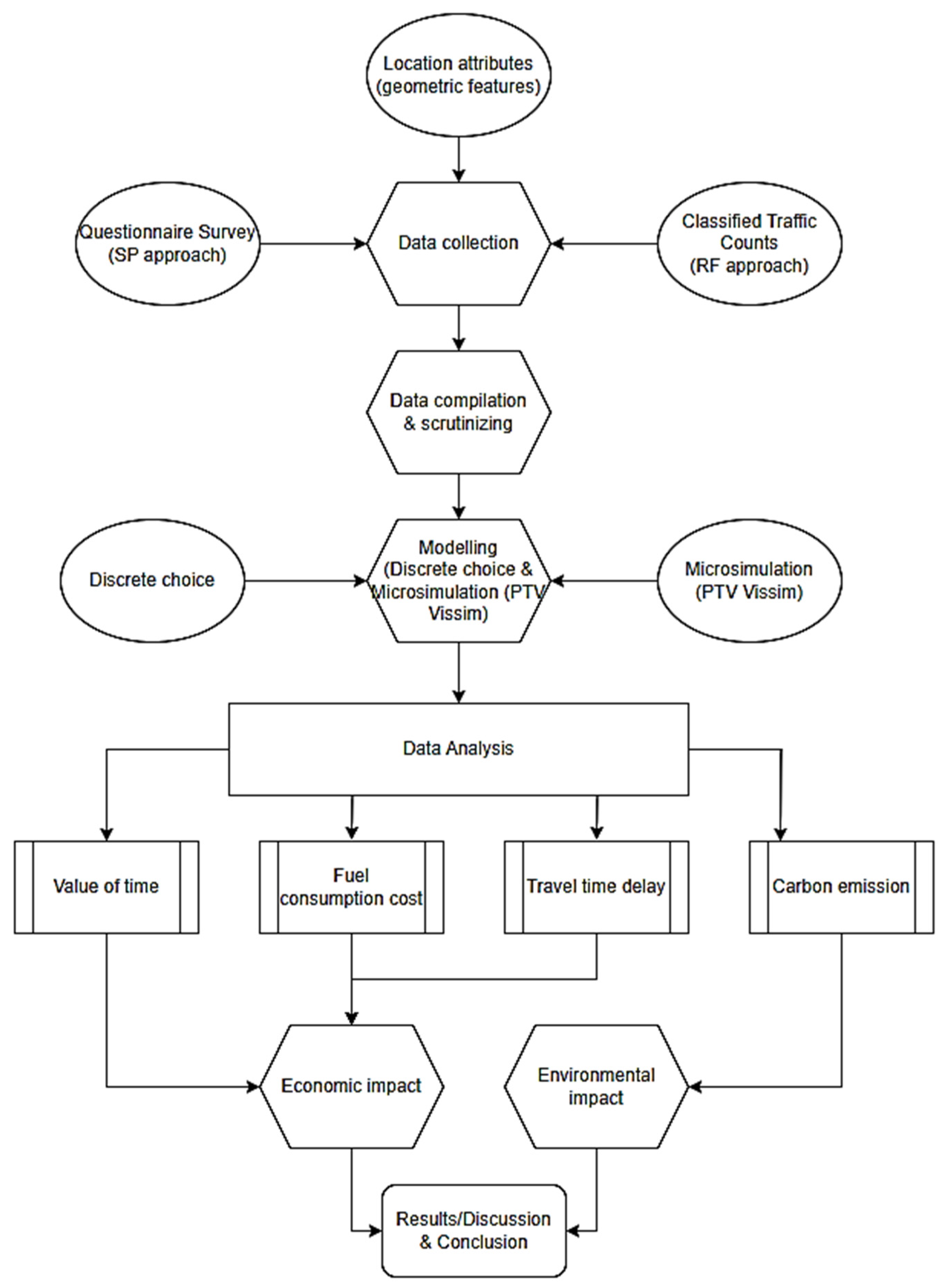
A stated preference (SP) approach was used to estimate VOTT, while travel delay and carbon emissions due to congestion caused by VIP movements were calculated using simulation in VISSIM. The detailed methodology adopted to complete the research objectives of this study is shown in Figure 2, and it includes an SP questionnaire structured to take advantage of its positive aspects, such as flexible experimental design and inclusion of nonexistent alternatives, as mentioned in the literature review. The guidelines provided by Wattam et al. to create such a survey were also utilized [55]. The questionnaire comprised four sections: demographic information, daily trip information, VIP movements, and preference questions.
Each respondent’s socioeconomic and demographic information was recorded in Section 1. Section 2 consisted of questions related to trips taken most frequently, including trip purpose, frequency per week, and average duration. Section 3 included queries about respondents’ experience with VIP movements. In Section 4, everyone was presented with four distinguishable routes and asked about the preferred mode of transportation. Each mode choice was equipped with various combinations of three parameters: travel cost, journey travel time, and waiting time in case of using public transport.

3.3. Data Collection

3.3.1. Stated Preference Survey

A questionnaire designed in the first step was used for the SP survey, which was conducted primarily based on convenience sampling and partially on snowball sampling techniques. Convenience sampling involves choosing easily accessible consumers to determine different socioeconomic factors affecting mode choice behavior and to collect choice data [56]. Snowball sampling is a non-probability technique in which sample subjects help the researcher recruit more sample subjects for the study [57], and it is beneficial for surveying hard-to-reach individuals [58]. Both traditional (pen and paper) and digital (Google Forms) platforms were utilized for this survey.

3.3.2. Traffic Counts Survey

The second data set included information about existing geometry (number of lanes, lane width, etc.), speed limits, signal timings, and traffic volumes for all five locations discussed in the study area. Data were collected through classified traffic counts conducted at each location during peak hours, from 7:00 a.m. to 10:00 a.m. and 4:00 p.m. to 8:00 p.m., and included different travel modes such as cars, motorcycles, and heavy vehicles (trucks).

3.4. Data Analysis

3.4.1. Discrete Choice Modeling

The selection of the unordered choice model, also known as the multinomial logit model, was based on the literature discussed in Section 2.1. This model is grounded in the theory of utility maximization, where each decision maker assigns a value to each option in the available choices and selects the one with the highest value. Since the exact value cannot be directly observed, a probabilistic approach is employed, giving rise to the random utility theory [59].
We adopt Equations (1)–(4) from K. E. Train to formulate and estimate a simple multinomial logit model. In this model, each decision maker (denoted as n) associates a utility U n , i   value with alternative i [59]. This utility value comprises two components: a deterministic or observable utility V n , i   , and a random or error component ε n , i . The deterministic utility is determined by the observed variables x n i   for alternative i. The probability of decision maker “n” choosing alternative i can be calculated using Equation (2):
U n , i = V n , i + ε n , i         w h e r e     V n , i = f β , x n i
P n i = P r o b   ( V n , i + ε n , i     V n , j + ε n , j     j )
The error terms associated with all the alternatives are assumed to be independently and identically distributed. In this case, a type 1 extreme value distribution, commonly known as a Gumbel distribution, is utilized [60]. This distribution allows for a mathematical expression that enables the modeling and analysis of the multinomial logit model. The model parameters, represented by β in f β , x n i , are estimated by maximizing the log-likelihood (LL) function (Equation (4)). Research conducted by D. McFadden and P. Zarembka has shown that the log-likelihood function exhibits global concavity, implying that a single and unique solution exists [61].
P n i = e V n i   j = 1 J e V n , j          
L L   β = n = 1 N i y n i l n ( P n i )  
where y n i is the observed choice
The general formulation of the utility function in the present study’s case is given by Equation (5):
U = β 0 + β t i m e . T T + β c o s t T C +            
where
  • β0: Intercept;
  • TC: Travel cost;
  • TT: Travel time;
  • βcost: Coefficient of travel cost (utility/Rs.);
  • βtime: Coefficient of travel time (utility/min);
  • “…”: Corresponds to other explanatory variables of the model.
Afterward, using the derived coefficient of travel cost and travel time, VOTT was estimated using Equation (6). The calculated value was in Pakistani rupees (PKR)/min, converted to USD/min:
V O T T = β t i m e β c o s t        

3.4.2. Microsimulation

The existing traffic conditions at all five locations were modeled in VISSIM using data from the traffic count survey. To accurately represent real-world scenarios, satellite images of the locations were integrated as background references and meticulously scaled to match on-site conditions. Subsequently, links and connectors were drawn based on geometric design data obtained from the field survey. Throughout the simulation, default settings for vehicle dimensions were applied, and traffic volume was allocated at the start of each road segment. Additionally, speed data collected during the survey were utilized to calibrate the model, ensuring that vehicle speeds within the simulation accurately reflected those observed on the field.
Furthermore, the traffic composition was determined based on the data gathered during the vehicle count survey, ensuring a realistic representation within the simulation environment. The Poisson distribution was used to load the assigned traffic volume randomly [62]. The results presented for each variant are based on an average of five simulation runs.
The first step in this study was to model and simulate existing conditions for each location in VISSIM v7. Signalized intersections were analyzed using existing signal timings, while free segments were simulated with all green signals. A psychophysical driver behavior model developed by Wiedemann (Mannheim, Germany) was used as the basis of car-following and lane-changing logic [63]. Node evaluation was employed to estimate carbon emissions and fuel consumption. Oak Ridge National Laboratory’s data on emissions [64], and the TRANSYT v7-F program’s formulas for fuel consumption, were utilized in node evaluations [65]. In the second step, a scenario of blockades due to VIP movement was created by introducing a red–green signal on all lanes of roads at all five locations in the VISSIM model. The red time was increased by two minutes in each simulation cycle to evaluate the impact of different stoppage time durations on various measures of effectiveness.

3.4.3. Economic Impact Analysis

Delay per vehicle, fuel consumption, and VOTT were used to estimate the economic impact of congestion caused by VIP movements. The travel time delay and fuel consumption costs were calculated for each scenario, and the total cost of road blockage was determined by adding these two costs (using discrete modeling) together:
T D C = T T D C + F C C            
Equation (8) was used to measure the delay cost of this study. The approach imposes VOTT on the calculated delay, and is a widely accepted method [50]:
T T D C = T T D × V O T T × N  
where
  • TTDC: Travel time delay cost;
  • TTD: Simulated travel time delay;
  • VOTT: Value of travel time;
  • N: Number of vehicles.
The vehicle operating cost or fuel loss cost is determined by multiplying the fuel cost with the additional fuel consumed by a vehicle while stuck in congestion. Fuel consumption analysis in VISSIM was used in this study to calculate the extra fuel consumed due to road blockages. The economic loss due to fuel was then calculated by multiplying fuel loss with the prevailing fuel cost:
F C C = ( F C × f c )  
where
  • FCC: Fuel consumption cost;
  • FC: Fuel consumption;
  • fc: Fuel cost.

3.4.4. Environmental Impact Analysis

The environmental impact of road blockages for VIP movements was assessed by comparing the amount (quantity) of pollutants emitted during different durations (time) of blockades. In this study area, all blockades were analyzed using VISSIM to estimate the emissions of pollutants (e.g., CO, NOx, and VOCs (volatile organic compounds)).

4. Results and Discussion

4.1. Sample Characteristics

A group of 445 individuals participated in the survey, but only 401 unique entities were selected for data analysis after scrutinizing responses for missing information and incomplete surveys. Of the selected respondents, 340 (85%) were male and 61 (15%) were female. Approximately 211 (53%) of respondents were between 20 and 30. Regarding income, most respondents (78%) reported monthly earnings below forty thousand Pakistani Rupee (PKR). Geographically, the majority (62%) of respondents were from Islamabad, Pakistan. Table 1 provides a detailed demographic breakdown of the respondents.

4.2. Traffic Volumes Used for Analysis

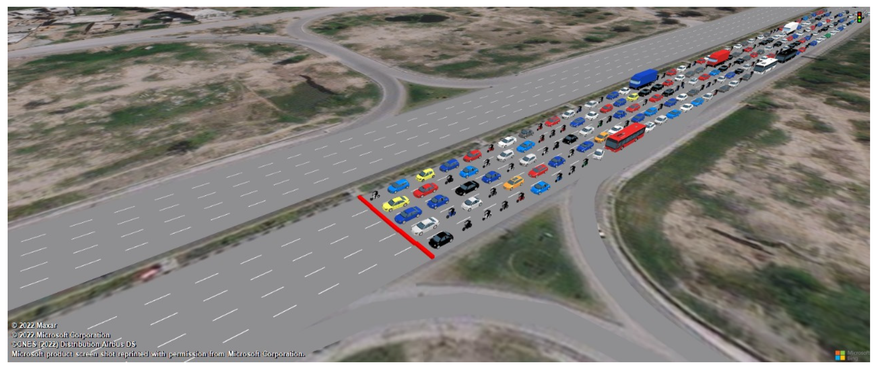
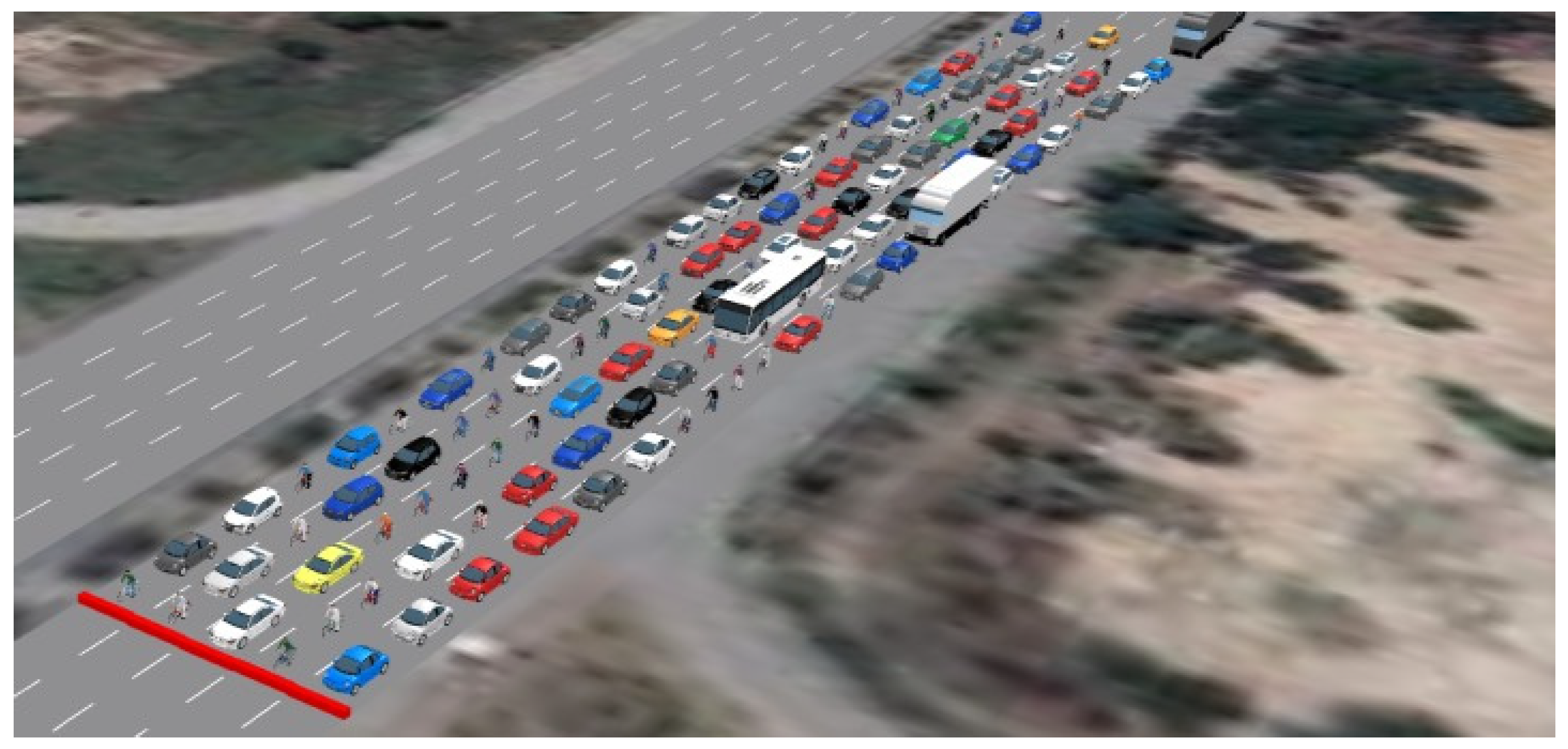
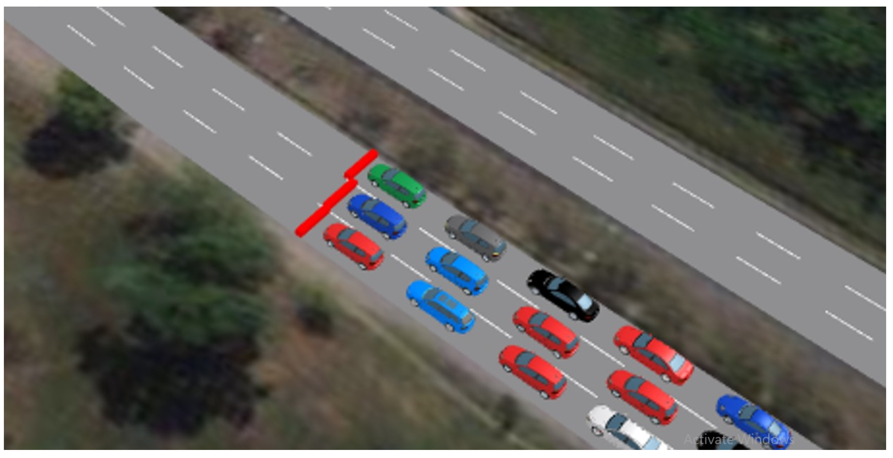
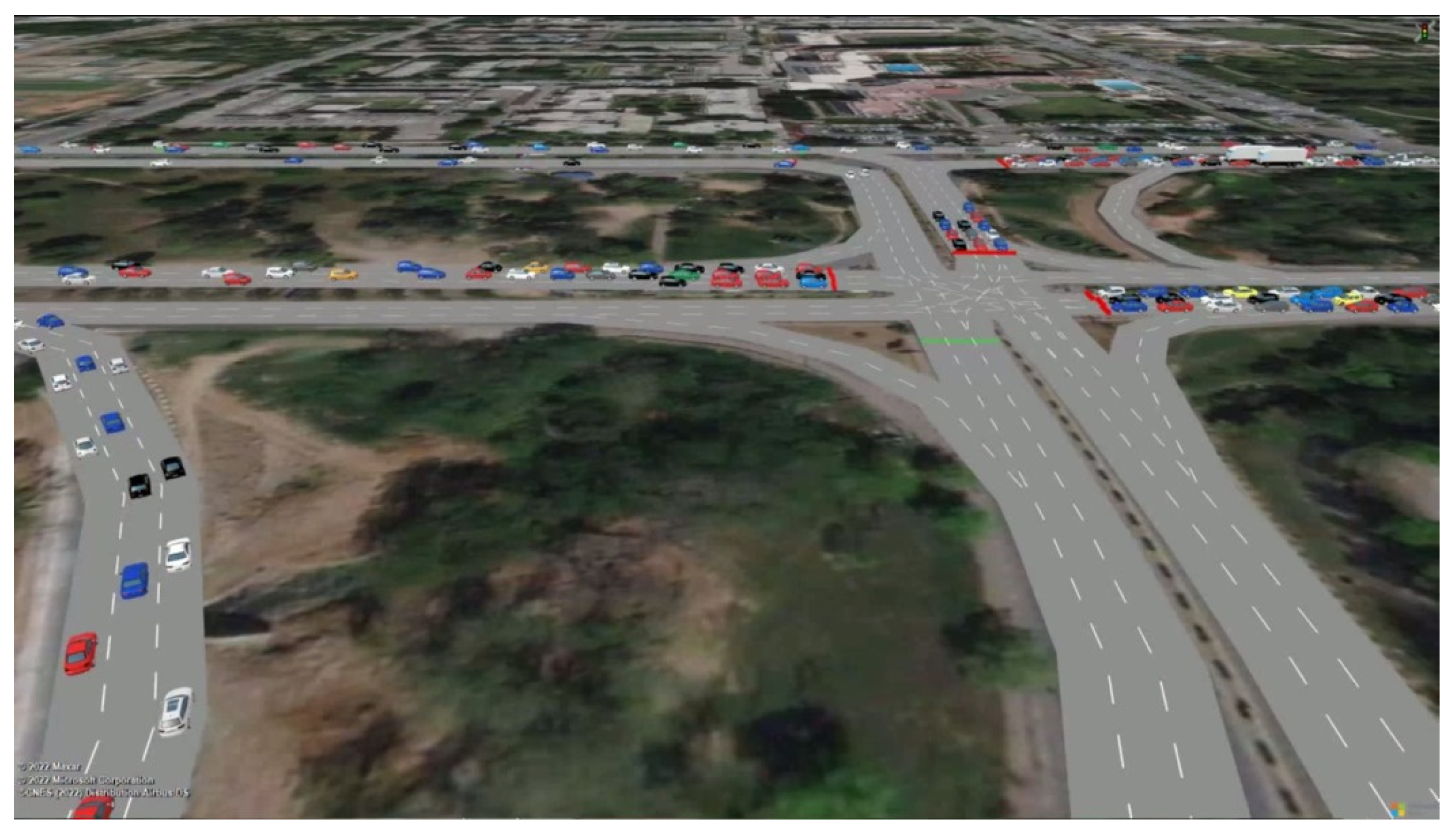
In the VISSIM v7 simulation, we relied on peak hour volumes on each intersections obtained from a comprehensive traffic count survey as crucial inputs as shown in Figure 3, Figure 4, Figure 5, Figure 6 and Figure 7 below. Additionally, the composition of vehicles in the simulation directly mirrored the data collected during the study.
These approaches ensured that our simulation accurately represented real-world traffic scenarios. We also incorporated speed limit data into the calibration process to further enhance the accuracy of our VISSIM simulation. Table 2 summarizes the survey’s traffic counts and the corresponding speed limits for calibrating the VISSIM model.
Furthermore, turning movements at signalized intersections were meticulously recorded, with detailed information shown in Table 3. By capturing turning movements, we gained insight into the directional flow of traffic within the intersection, allowing for a more comprehensive analysis of traffic patterns and signal operation. Additionally, we utilized the recorded existing signal timing to faithfully depict the current conditions within the simulation. By incorporating these timings, we ensured an accurate representation of real-world traffic operations, enhancing the reliability and effectiveness of our VISSIM simulation.

4.3. Choice Model Estimation

The model was implemented and estimated with the Apollo choice modeling library in the R language [66]. Initially, only the primary variables of travel cost and travel time were included in the model specification. Relevant explanatory variables were incrementally added to the model based on summary goodness of fit measures, such as log-likelihood and AIC, and the significance of the estimated parameter coefficients. The steps and probability values of corresponding likelihood ratio tests are listed in Table 4.
Initially, coefficients of travel cost and travel time were generic for all choices. Then, the beta (β) coefficients of travel time were varied for each mode, but the log-likelihood test was found to be statistically insignificant. Therefore, the first model was adopted over the second. Gender was included in the utility function, first generically and then separately for each mode, where the β coefficients were statistically significant in both cases. However, a better log-likelihood was achieved in the second case.
Age as a contributing variable was statistically insignificant in the utility function for all modes. Categorizing age into different groups did not result in significant β coefficients or log-likelihood improvement; therefore, age was not included in the final model. In contrast, a high-income category was introduced for individuals with an income of 60 thousand or more, and the maximum log-likelihood was achieved by introducing a high-income coefficient for cars.
The final model results, reported in Table 5, show that all coefficients are significant at the 99% confidence interval except for income, which is statistically significant at the 90% confidence interval, as shown in the t-value of income. The negative coefficients for travel time and cost and the meaningful VOTT indicate a good fit for the model.
Interestingly, the coefficient of gender (female) is negative for bikes, indicating that women have a strong preference for cars over bikes. In contrast, the coefficient of gender (female) is positive for vans, suggesting that women prefer vans over vehicles. The positive coefficient for the high-income category indicates that as income increases, the probability of choosing a car over other modes of transportation also increases.
Table 6 displays the calculated VOTT estimated using Equation (6). The VOTT was determined to be 396 PKR/h, equivalent to 1.77 USD/h. This value falls within the previous value of time studies [39,67] carried out in Pakistan, whose VOTT estimates were 0.41 USD/h and 3.67 USD/h, respectively. Since both previous studies were carried out in Karachi, the slight difference in the results of the current study may be due to demographic variation between the locations of the three studies.

4.4. Simulation Results

4.4.1. Freeway Segments

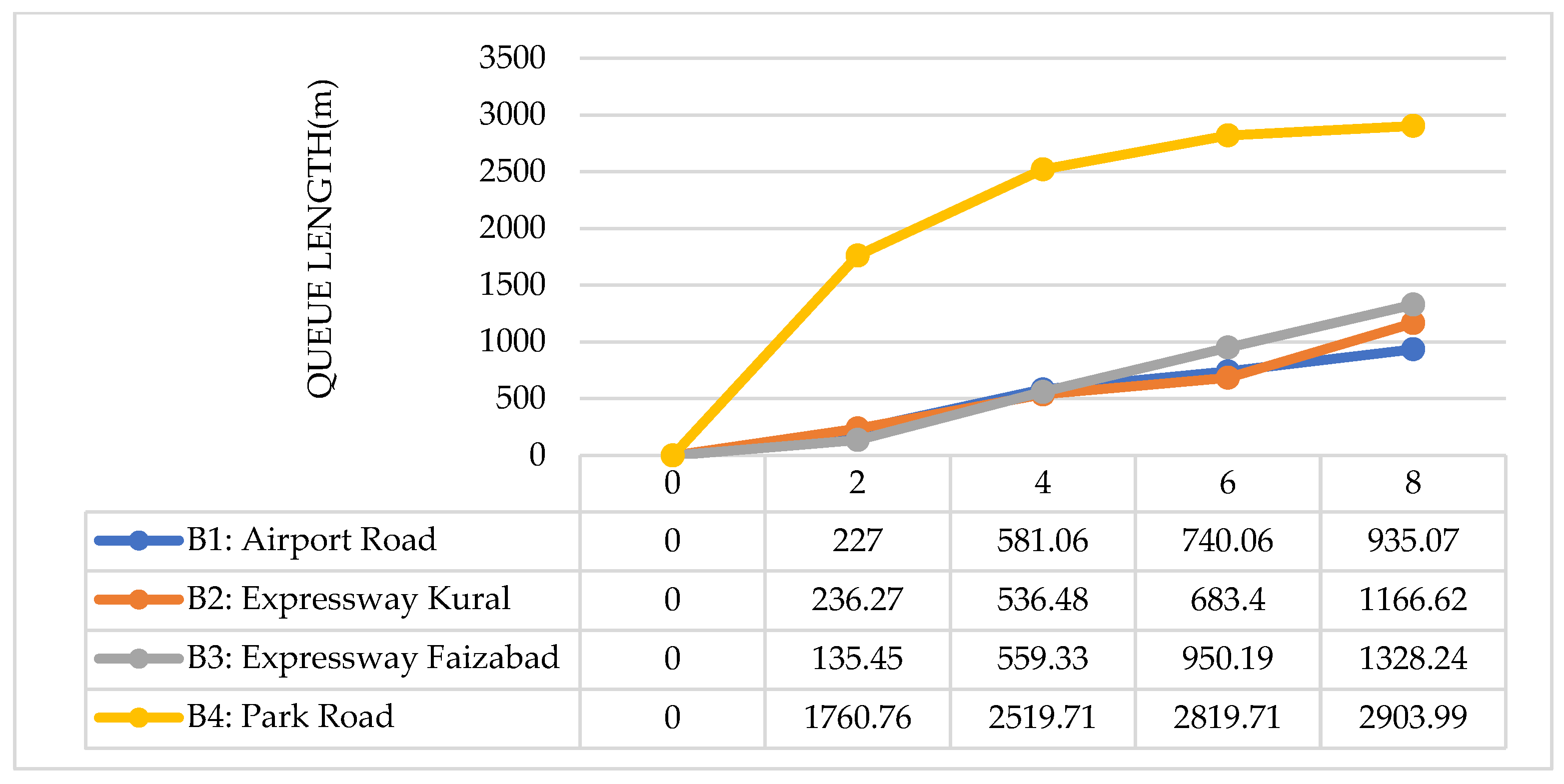
In Figure 8, the simulation portrays the progression of queue length at freeway sections corresponding to each blockade time. Initially, all freeway locations exhibited zero queue length, as simulated. Subsequently, the queue length increment was gradual for blockades 1 to 3, situated along multilane divided highways. However, at blockade 4, simulated on the two-lane divided urban arterial named Park Road, the queue experienced exponential growth.
Figure 9 depicts the simulation results of delay per vehicle for each blockade interval at freeway segments. Initially, delays were nonexistent at each simulated location. However, as the simulation’s blockade time exceeded two minutes, the delay per vehicle sharply increased.

4.4.2. Signalized Intersection

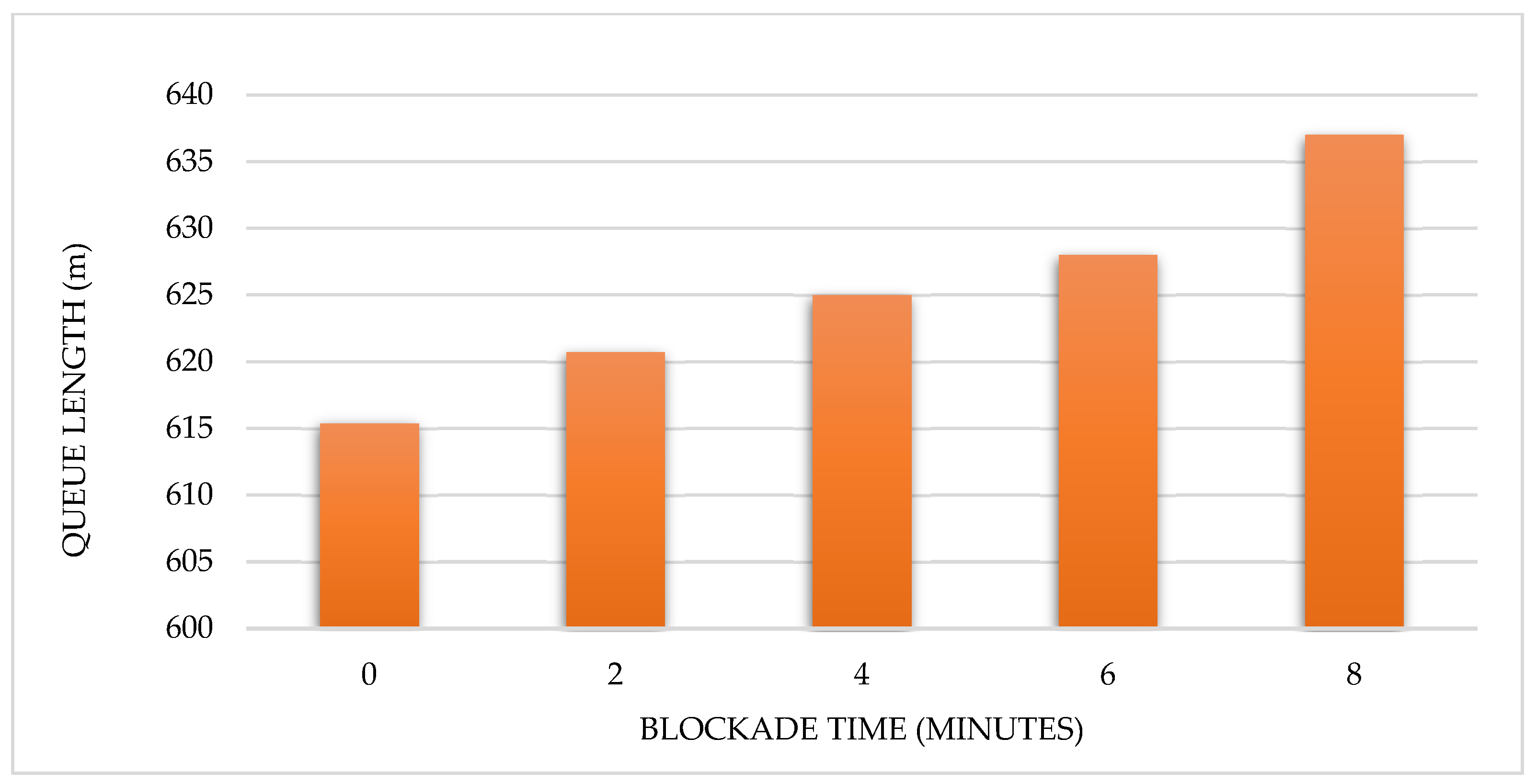
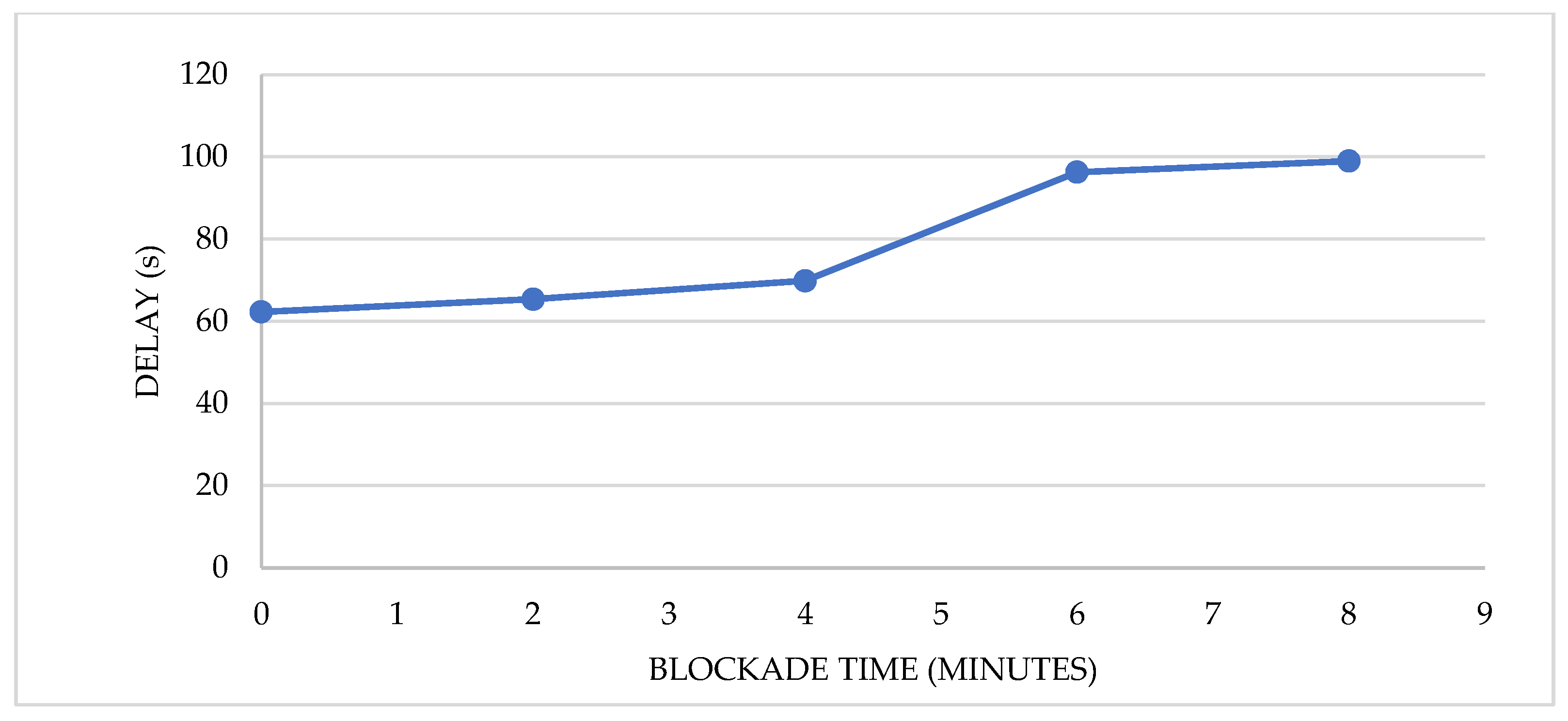
Figure 10 and Figure 11 present the simulation results from VISSIM, showcasing the influence of different blockade intervals on delay and maximum queue length at an existing signalized intersection.

4.4.3. Economic Impact Analysis

The economic impact of traffic congestion caused by VIP movements was calculated using VOTT, estimated in the previous section, along with the travel delay and additional fuel consumption estimated via microsimulation. The microsimulation analysis was divided into variant 0, where the current state was modeled, and variants 1–4, where 2 min of blockade time were added for each variation, and the blockade time was incremented gradually from 2 to 8 min. This was conducted to model the impact of blockade time on travel time delay and fuel consumption of vehicles stuck in congestion.

4.4.4. Existing Delay Cost (Variant 0)

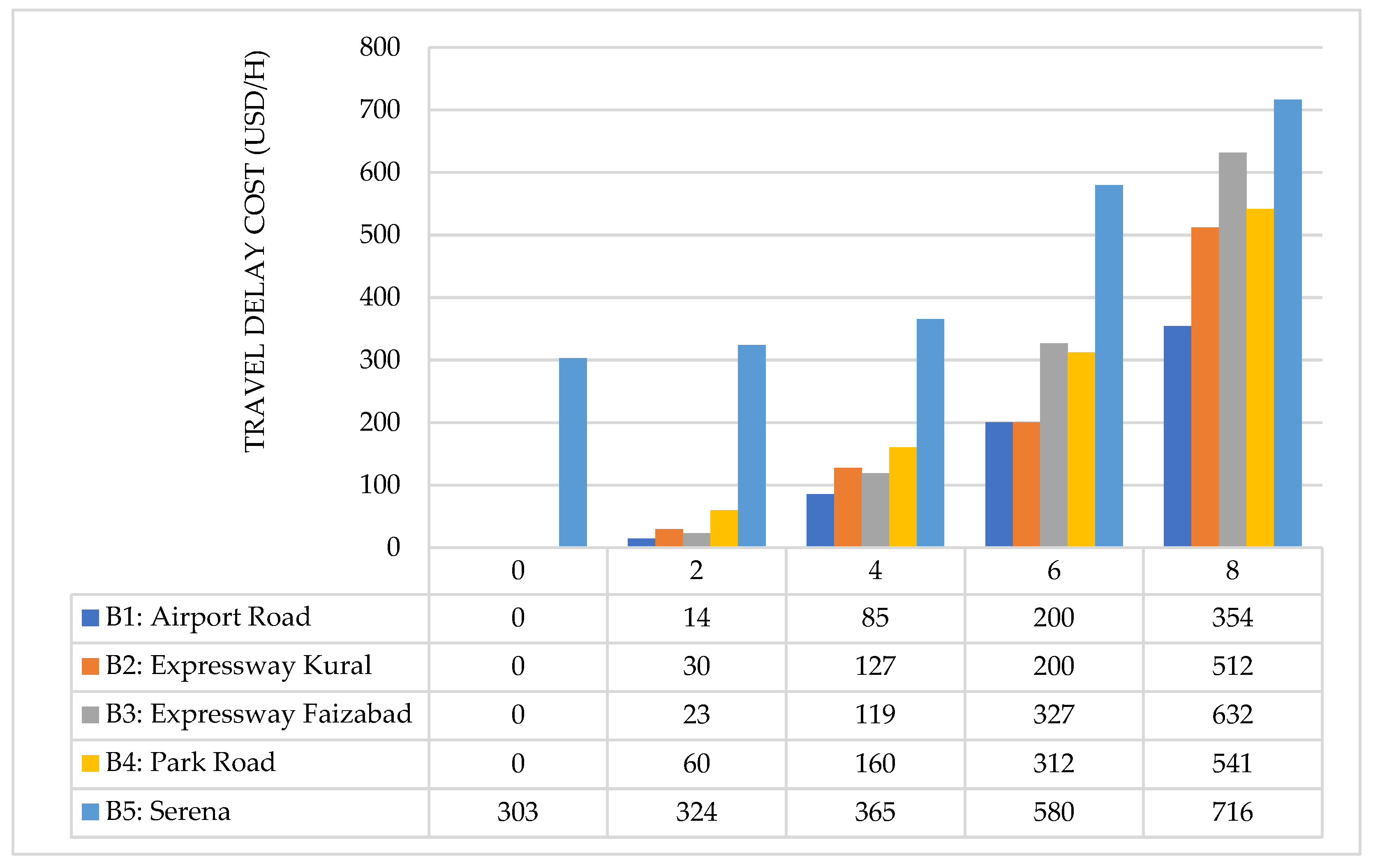
The travel time delay cost (TTDC) was estimated using Equation (8), and the results of each variation of a blockade at all locations are shown in Figure 12. The existing delay cost was estimated to be 303 USD/h (67,650 PKR/h) at B5-Serena, while the delay cost was zero at all other locations due to them being freeway segments.

4.4.5. Scenario Runs (Variants 0–4)

The blockade time is indicated for each variation along the x-axis of Figure 12. The results indicate a slight increase in travel delay cost as the stoppage time increases from zero to 2 min. However, the travel delay cost almost quadruples as the blockade time is increased from 2 min to 4 min. The only exception to this sudden increment is the B5 intersection, where the increase, though significant, is a little less drastic.

4.5. Fuel Consumption Cost

Fuel consumption analysis was conducted using VISSIM to estimate the impact of different blockade timings on fuel consumption. The fuel loss cost for different blockade intervals was calculated by multiplying fuel consumed by the average fuel cost for the last six months. Table 7 shows the variation in fuel consumption cost concerning different blockade times estimated using Equation (9). The table shows each variant’s total fuel utilized at all five locations.

4.6. Total Cost of Delay

Table 8 illustrates the variation in total delay cost for different blockade interval estimates using Equation (7). The total delay cost was calculated by adding the estimated travel delay and fuel loss costs from the previous two sections.
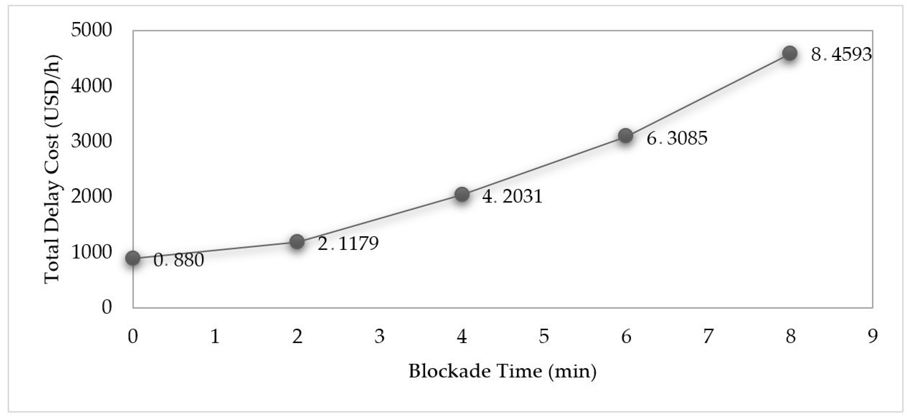
Figure 13 indicates that the total delay cost increases gradually with an increase in the blockage time from zero to two minutes. However, beyond two minutes, the increase in delay cost rate becomes steeper. During the initial two minutes, the rate of increase is 149.5 USD/h (33,338 PKR/h) for every minute of blockade time. This rate doubles to 425 USD/h (94,775 PKR/h) when the blockade time exceeds two minutes and approaches four minutes.

4.6.1. Environmental Impact Analysis

Like the travel delay and fuel consumption analysis, this analysis was also divided into variant 0 where the current state was modeled, and variants 1–4, where 2 min of blockade time was added for each variation to model the impact of different blockade times on exhaust emission of vehicles.

4.6.2. Existing State (Variant 0)

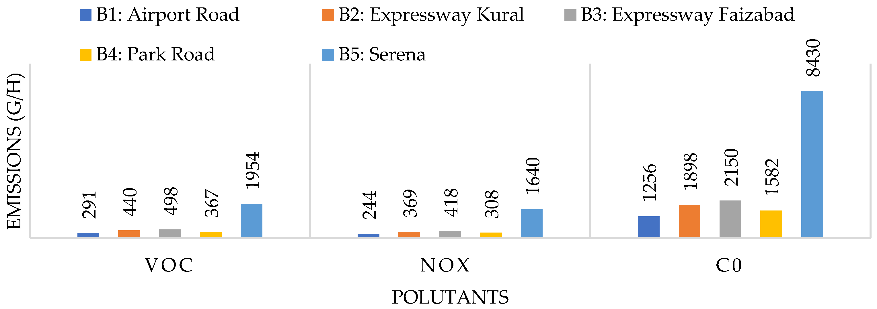
The microsimulation models of the existing state produce different results for each location due to variations in traffic volumes, vehicle composition, and road geometry at each location. Figure 14 shows the existing emission level of each pollutant at individual locations. The highest emission levels for CO pollutants were measured at B-5 near Serena, with a value of 8430 g/h, while for all other places, this value was around or below 200 g/h.
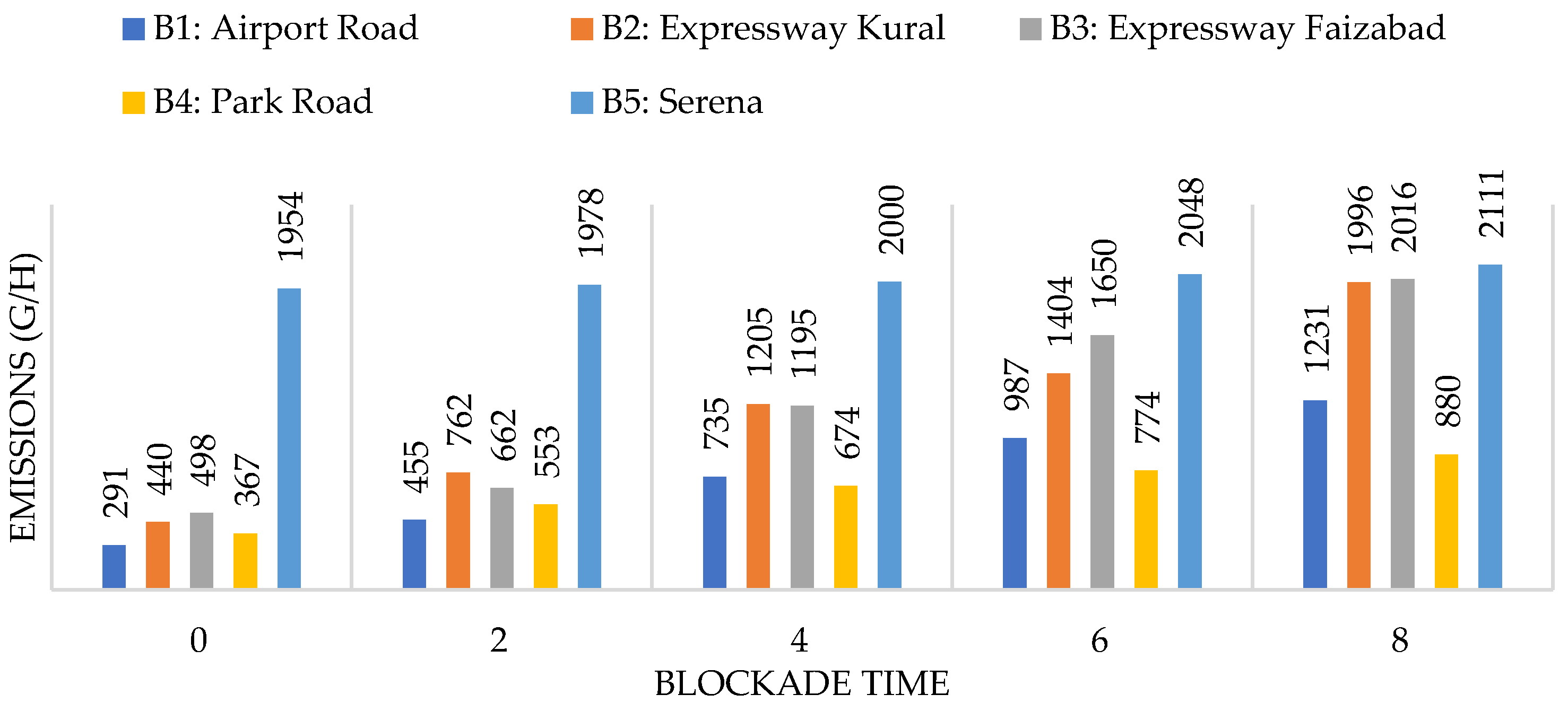
The existing NOx and VOC emission levels were also highest near Serena, similar to CO. At B-5, the quantity of NOx recorded was 1640 g/h and that of VOC was 1954 g/h, while at all other locations, these values were below 500 g/h. This variation in measurement is due to the presence of an existing traffic signal at B-5 near Serena.

4.6.3. Scenario Runs (Variants 0–4)

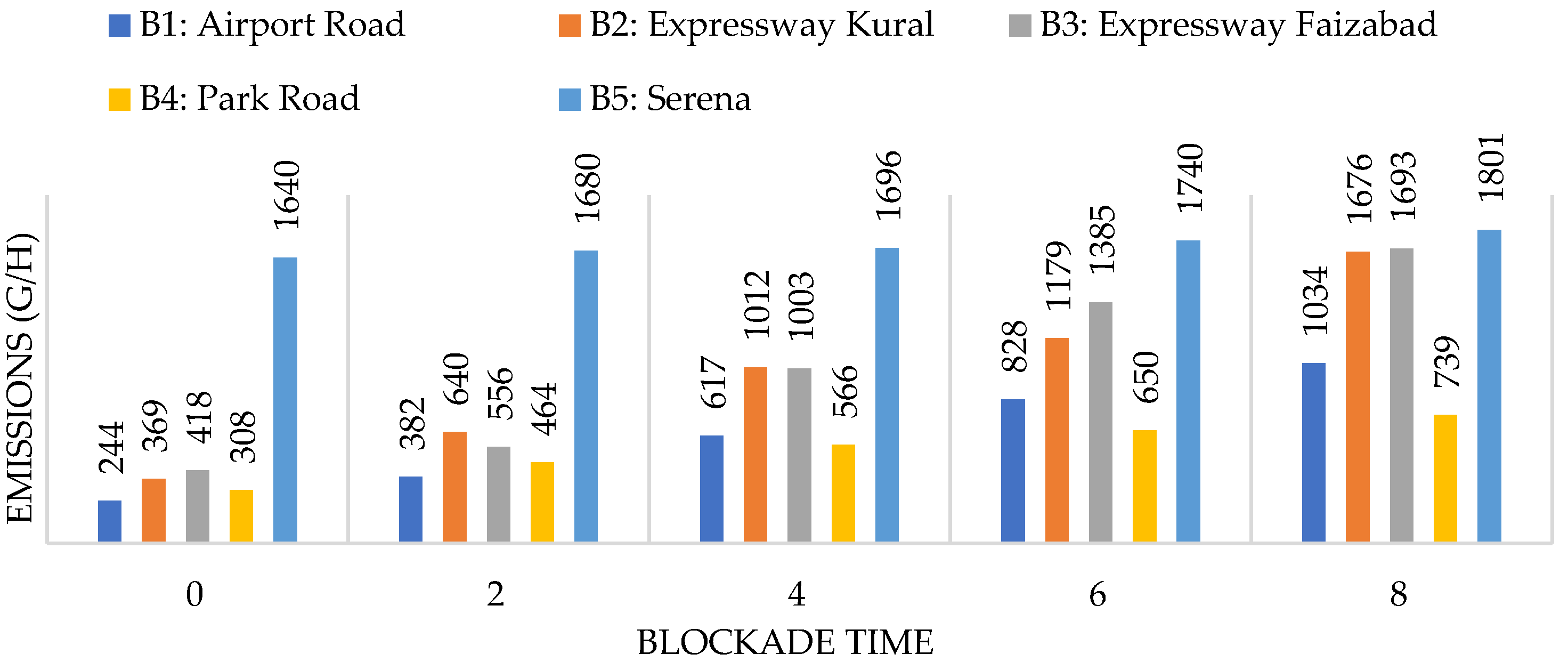
The simulation results indicate that emissions of all three pollutants increase with blockade time. Figure 15, Figure 16 and Figure 17 shows the variation in emissions of individual pollutants with different blockade time intervals at each location. The x-axis of each figure shows the blockade time, which ranges from zero minutes for variant 0 to 8 min for variant 4. The emission of pollutants increased linearly with stoppage time at blockades 1 to 5. Analysis of the individual sum of exhaust emissions indicates that as blockade time increases, blockade B1–B4 emissions rise more sharply than those of B5.

5. Discussion and Conclusions

This study explored the environmental and economic impacts of road blockages due to VIP movements in urban areas. Notably, travel time and cost emerged as crucial factors influencing mode choice, alongside gender and income. While women generally preferred cars over bikes, they tended to opt for public transport during VIP movements. Moreover, individuals with incomes exceeding 60 thousand rupees were more inclined towards car use. However, age did not affect mode choice significantly in this context. The value of travel time (VOTT) estimated at 397 PKR/h (1.77 USD/h) closely mirrored previous studies [39,67], suggesting that VIP-induced blockage incurs costs comparable to congestion in metropolitan cities.
Microsimulation results demonstrated the detrimental effect of VIP blockages on the environment and transportation system. Carbon emissions and fuel consumption increased substantially with prolonged blockage durations, which was particularly noticeable at freeway segments compared to signalized intersections. Moreover, the exponential growth in delay costs (from 34% in the first two minutes to 72% in the next two minutes) and exhaust emissions highlighted the negative impact of VIP movements on the economy and the well-being of road users, especially in developing countries.
A critical policy recommendation from this research is to restrict VIP blockages to a maximum of two minutes. Additionally, the study emphasizes the importance of implementing sustainable transportation policies to discourage private car usage. Despite the valuable insights provided, it is critical to acknowledge certain limitations. The contextual nature of the findings may not fully encompass the complexity of all urban settings, and the modeling approach’s reliance on assumptions could affect result accuracy. Nonetheless, the study emphasizes the urgent need for sustainable transportation policies and offers valuable recommendations for policymakers to enhance the well-being of road users in developing nations.

Author Contributions

Conceptualization, M.A.J. and S.U.-D.; methodology, M.A.J., S.U.-D., M.U.Z., M.S.M. and M.A.K.; software, M.A.J., S.U.-D. and M.A.K.; validation, S.U.-D., M.U.Z. and M.A.K.; formal analysis, M.A.J., M.S.M. and S.U.-D.; investigation, M.A.J.; resources, S.U.-D.; data curation, M.U.Z., M.A.K. and A.A.; writing—original draft preparation, M.A.J., S.U.-D. and A.A.; writing—review and editing, M.A.J., S.U.-D., M.U.Z., M.S.M. and A.A.; supervision, S.U.-D. and M.U.Z.; project administration, M.A.J. and S.U.-D. All authors have read and agreed to the published version of the manuscript.

Funding

This work was supported by the Deanship of Scientific Research, Vice Presidency for Graduate Studies and Scientific Research, King Faisal University, Saudi Arabia (GRANT No. KFU 241054). The APC was funded by the same “Grant No. KFU241054”.

Institutional Review Board Statement

The committee reviewed responses to the conditions placed upon the ethical approval. This study proposal is now deemed to meet the requirements of the Ethics in Engineering (1983), and full ethical approval has been granted. Approval No. ACAD/R/E/20210630 by Departmental Ethics Sub-Committee at School of Civil and Environmental Engineering, National University of Sciences and Technology, H-12 Campus, 44000, dated 9 July 2021.

Informed Consent Statement

Written informed consent was obtained from the participant(s) to conduct the survey for this study.

Data Availability Statement

All or some data, models, and code will be provided upon reasonable request to the corresponding author.

Acknowledgments

The authors acknowledge the Deanship of Scientific Research, Vice Presidency for Graduate Studies and Scientific Research, King Faisal University, Saudi Arabia (GRANT No. KFU241054). The authors extend their appreciation for the financial support that has made this study possible.

Conflicts of Interest

The authors declare that they have no known competing financial or non-financial interests or other interests that might be perceived to influence the results and/or Discussion reported in this paper.

References

  1. Malibari, A.; Higatani, A.; Saleh, W. Assessing the Impacts of Autonomous Vehicles on Road Congestion Using Microsimulation. Sensors 2022, 22, 4407. [Google Scholar] [CrossRef] [PubMed]
  2. Fernando, R. The impact of Planned Special Events (PSEs) on urban traffic congestion. ICST Trans. Scalable Inf. Syst. 2018, 6, 159624. [Google Scholar] [CrossRef]
  3. Kong, X.; Xu, Z.; Shen, G.; Wang, J.; Yang, Q.; Zhang, B. Urban traffic congestion estimation and prediction based on floating car trajectory data. Future Gener. Comput. Syst. 2016, 61, 97–107. [Google Scholar] [CrossRef]
  4. Yang, Q.; Gao, Z.; Kong, X.; Rahim, A.; Wang, J.; Xia, F. Taxi Operation Optimization Based on Big Traffic Data. In Proceedings of the 2015 IEEE 12th International Conference on Ubiquitous Intelligence and Computing and 2015 IEEE 12th International Conference on Autonomic and Trusted Computing and 2015 IEEE 15th International Conference on Scalable Computing and Communications and Its Associated Workshops (UIC-ATC-ScalCom), Beijing, China, 10–14 August 2015; pp. 127–134. [Google Scholar] [CrossRef]
  5. Zhao, J.; Li, R.; Liang, X.; Xu, K. Second ring is the most jammed road in Beijing: A view from taxis and Weibo. In Proceedings of the 2016 13th International Conference on Service Systems and Service Management (ICSSSM), Kunming, China, 24–26 June 2016; pp. 1–6. [Google Scholar] [CrossRef]
  6. Karuppanagounder, K. Economic Impact of Traffic Congestion-Estimation and Challenges. Eur. Transp./Trasp. Eur. 2018, 68, 1–19. [Google Scholar]
  7. Department of Transport and Regional Services. Estimating Urban Traffic and Congestion Cost Trends for Australian Cities; Bureau of Transport and Regional Economics: Canberra, Australia, 2007; No. 71.
  8. Weisbrod, G.; Vary, D.; Treyz, G.; Goodwin, P.; ESRC Transport Studies Unit University College London. The Economic Costs of Road Traffic Congestion; University College London: London, UK, 2003; pp. 98–106. [Google Scholar]
  9. Garrido, N. Computing the cost of traffic congestion: A microsimulation exercise of the City of Antofagasta, Chile. Transp. Plan. Technol. 2012, 35, 752–768. [Google Scholar] [CrossRef]
  10. Khan, T.; Islam, M.R. Estimating Costs of Traffic Congestion in Dhaka City. Int. J. Eng. Sci. Innov. Technol. 2013, 2, 281–289. [Google Scholar]
  11. Ali, M.S.; Adnan, M.; Noman, S.M.; Baqueri, S.F.A. Estimation of traffic congestion cost—A case study of a major arterial in Karachi. Procedia Eng. 2014, 77, 37–44. [Google Scholar] [CrossRef]
  12. Yugihartiman, M.; Budiono, B.; Setiawan, M.; Hidayat, A.K. Estimating Travel Choice Probability of Link-Based Congestion Charging Scheme for Car Commuter Trips in Jakarta. Sustainability 2023, 15, 8104. [Google Scholar] [CrossRef]
  13. Oszczypała, M.; Ziółkowski, J.; Małachowski, J.; Lęgas, A. Nash Equilibrium and Stackelberg Approach for Traffic Flow Optimization in Road Transportation Networks—A Case Study of Warsaw. Appl. Sci. 2023, 13, 3085. [Google Scholar] [CrossRef]
  14. Munir, T.; Dia, H.; Shafiei, S.; Ghaderi, H. Comparative Evaluation of Road Pricing Schemes: A Simulation Approach (Australian Perspective). Sustainability 2023, 15, 16366. [Google Scholar] [CrossRef]
  15. Andrei, L.; Luca, O.; Gaman, F. Insights from User Preferences on Automated Vehicles: Influence of Socio-Demographic Factors on Value of Time in Romania Case. Sustainability 2022, 14, 10828. [Google Scholar] [CrossRef]
  16. Bashingi, N.; Mostafa, M.; Kumar Das, D. The state of congestion in the developing world; The case of Gaborone, Botswana. Transp. Res. Procedia 2020, 45, 434–442. [Google Scholar] [CrossRef]
  17. Ali, A.; Ud-Din, S.; Saad, S.; Ammad, S.; Rasheed, K.; Ahmad, F. Artificial Neural Network Approach to Study the Effect of Driver Characteristics on Road Traffic Accidents. In Proceedings of the 2021 International Conference on Data Analytics for Business and Industry (ICDABI), Sakheer, Bahrain, 25–26 October 2021; pp. 277–280. [Google Scholar] [CrossRef]
  18. Pakistan Bureau of Statistics. Salient Features of Final Results Census-2017; Pakistan Bureau of Statistics: Islamabad, Pakistan, 2017.
  19. Independent Evaluation Office. Assessment of Development Results Evaluation of UNDP Contribution Pakistan; UNDP 2017; United Nations Development Programme: Islamabad, Pakistan, 2017. [Google Scholar]
  20. Ben-Akiva, M.E.; Lerman, S.R. Discrete Choice Analysis: Theory and Application to Travel Demand; MIT Press: Cambridge, MA, USA, 1985. [Google Scholar]
  21. Ramjerdi, F.; Rand, L.; Sætermo, I.A.F.; Sælensminde, K. The Norwegian Value of Time Study Part I; Institute of Transport Economics: Oslo, Norway, 1997. [Google Scholar]
  22. Corthout, J.; Pieters, L.; Claeys, M.; Geerts, S.; Berghe, D.V.; Vlietinck, A. Antibacterial and molluscicidal phenolic acids from Spondias mombin. Planta Medica 1994, 60, 460–463. [Google Scholar] [CrossRef] [PubMed]
  23. Gunn, H.; Bradley, M.; Rohr, C. The 1994 national value of time study of road traffic in England (draft paper). In Proceedings of the Value of Time Seminar, London, UK, 29–30 October 1996; Volume Session 2. [Google Scholar]
  24. Axhausen, K.W.; König, A.; Abay, G.; Bates, J.J.; Bierlaire, M. Swiss Value of Travel Time Savings. In Proceedings of the European Transport Conference, Strasbourg, France, 4–6 October 2004. [Google Scholar]
  25. Schmid, B.; Molloy, J.; Peer, S.; Jokubauskaite, S.; Aschauer, F.; Hössinger, R.; Gerike, R.; Jara-Diaz, S.R.; Axhausen, K.W. The value of travel time savings and the value of leisure in Zurich: Estimation, decomposition and policy implications. Transp. Res. Part A Policy Pract. 2021, 150, 186–215. [Google Scholar] [CrossRef]
  26. Wardman, M. The value of travel time: A review of British evidence. J. Transp. Econ. Policy 1998, 32, 285–316. [Google Scholar]
  27. Diamandis, P.F.; Kouretas, G.P.; Tzanetos, P. Modelling the choice of mode and estimation of the value of travel time savings for the case of the Rion-Antirion suspension bridge in Greece. Ann. Reg. Sci. 1997, 31, 473–489. [Google Scholar] [CrossRef]
  28. Polydoropoulou, A.; Kapros, S.; Pollatou, E. A national passenger mode choice model for the Greek observatory. In Proceedings of the 10th World Conference on Transport Research, Istanbul, Turkey, 4–8 July 2004. [Google Scholar]
  29. Bierlaire, M.; Thémans, M. Development of Swiss models for transportation demand prediction in response to real-time traffic information. In Proceedings of the 5th Swiss Transport Research Conference, Ascona, Switzerland, 9–11 March 2005; p. 17. [Google Scholar]
  30. Kawamura, K. Perceived Value of Time for Truck Operators. Transp. Res. Rec. J. Transp. Res. Board 2000, 1725, 31–36. [Google Scholar] [CrossRef]
  31. Kurri, J.; Sirkiä, A.; Mikola, J. Value of Time in Freight Transport in Finland. Transp. Res. Rec. J. Transp. Res. Board 2000, 1725, 26–30. [Google Scholar] [CrossRef]
  32. Tao, X.; Zhu, L. Meta-analysis of value of time in freight transportation: A comprehensive review based on discrete choice models. Transp. Res. Part A Policy Pract. 2020, 138, 213–233. [Google Scholar] [CrossRef]
  33. Kumar, C.V.; Basu, D.; Maitra, B. Modeling Generalized Cost of Travel for Rural Bus Users: A Case Study. J. Public Transp. 2004, 7, 59–72. [Google Scholar] [CrossRef]
  34. Rizzi, L.I.; de Dios Ortúzar, J. Stated preference in the valuation of interurban road safety. Accid. Anal. Prev. 2003, 35, 9–22. [Google Scholar] [CrossRef] [PubMed]
  35. Rizzi, L.I.; de Dios Ortúzar, J. Road safety valuation under a stated choice framework. J. Transp. Econ. Policy 2006, 40, 69–94. [Google Scholar]
  36. Hensher, D.A.; Rose, J.M.; de Dios Ortúzar, J.; Rizzi, L.I. Estimating the willingness to pay and value of risk reduction for car occupants in the road environment. Transp. Res. Part A Policy Pract. 2009, 43, 692–707. [Google Scholar] [CrossRef]
  37. Antoniou, C. A stated-preference study of the willingness-to-pay to reduce traffic risk in urban vs. rural roads. Eur. Transp. Res. Rev. 2014, 6, 31–42. [Google Scholar] [CrossRef]
  38. González, R.M.; Marrero, Á.S.; Navarro-Ibáñez, M. Tourists’ travel time values using discrete choice models: The recreational value of the Teide National Park. J. Sustain. Tour. 2018, 26, 2021–2042. [Google Scholar] [CrossRef]
  39. Baqueri, S.F.A.; Ectors, W.; Ali, M.S.; Knapen, L.; Janssens, D.; Yasar, A.-U.-H. Estimation of Value of Time for a Congested Network—A Case Study of the National Highway, Karachi. Procedia Comput. Sci. 2016, 83, 262–269. [Google Scholar] [CrossRef]
  40. Louviere, J.J.; Hensher, D.A.; Swait, J.D. Stated choice methods: Analysis and application. In Stated Choice Methods; Cambridge University Press: Cambridge, UK, 2000; pp. 227–251. [Google Scholar]
  41. Bertini, R.L.; Lindgren, R.; Tantiyanugulchai, S. Application of PARAMICS Simulation at a Diamond Interchange; Research Report PSU-CE-TRG-02-02; Portland State University Transportation Research Group: Portland, OR, USA, 2002; p. 35. [Google Scholar]
  42. Owais, M.; Abulwafa, O.; Abbas, Y.A. When to Decide to Convert a Roundabout to a Signalized Intersection: Simulation Approach for Case Studies in Jeddah and Al-Madinah. Arab. J. Sci. Eng. 2020, 45, 7897–7914. [Google Scholar] [CrossRef]
  43. Hashmi, H.T.; Ud-Din, S.; Khan, M.A.; Khan, J.A.; Arshad, M.; Hassan, M.U. Traffic Flow Optimization at Toll Plaza Using Proactive Deep Learning Strategies. Infrastructures 2024, 9, 87. [Google Scholar] [CrossRef]
  44. Mosseri, G.M.S.; Hall, M.A.; Meyers, J.J. Vissim micro-simulation modeling of complex geometry and traffic control: A case study of Ocean Parkway, NY. In Proceedings of the ITE 2004 Annual Meeting and Exhibit, Lake Buena Vista, FL, USA, 1–4 August 2004. [Google Scholar]
  45. Gomes, G.; May, A.; Horowitz, R. Congested Freeway Microsimulation Model Using VISSIM. Transp. Res. Rec. J. Transp. Res. Board 2004, 1876, 71–81. [Google Scholar] [CrossRef]
  46. Vélez, E.G.; Díaz, D.M.V.; Villafañe, F.L. Evaluation of VISSIM a Dynamic Simulation Model for an Arterial Network at Mayagüez, Puerto Rico. In Proceedings of the Fourth LACCEI International Latin American and Caribbean Conference for Engineering and Technology, Mayagüez, Puerto Rico, 21–23 June 2006; pp. 1–11. Available online: http://www.laccei.org/LACCEI2006-PuertoRico/Papers-pdf/INF174_ValdesDiaz.pdf (accessed on 29 November 2021).
  47. Fabianova, J.; Michalik, P.; Janekova, J.; Fabian, M. Design and evaluation of a new intersection model to minimize congestions using VISSIM software. Open Eng. 2020, 10, 48–56. [Google Scholar] [CrossRef]
  48. Chen, C.; Zhao, X.; Liu, H.; Ren, G.; Zhang, Y.; Liu, X. Assessing the Influence of Adverse Weather on Traffic Flow Characteristics Using a Driving Simulator and VISSIM. Sustainability 2019, 11, 830. [Google Scholar] [CrossRef]
  49. Shi, J.Q.; Cheng, L. Simulation and Analysis of Highway Traffic Accident Based on VISSIM. Appl. Mech. Mater. 2012, 253–255, 1682–1685. [Google Scholar] [CrossRef]
  50. Bivina, G.R.; Landge, V.; Kumar, V.S.S. Socio Economic Valuation of Traffic Delays. Transp. Res. Procedia 2016, 17, 513–520. [Google Scholar] [CrossRef]
  51. Khan, M.A.; Ahmed, A.; Kayani, W.I.U.H. Optimal Timing for Lane(s) Addition to an Existing Highway: A Benefit–Cost Approach. Arab. J. Sci. Eng. 2019, 44, 4169–4182. [Google Scholar] [CrossRef]
  52. Karthik, S.; Loui, T.R. Development of Traffic Congestion Model to Evaluate the Level of Congestion and its Associative Cost for an Urban Arterial Road: A Case Study. J. Inst. Eng. Ser. A 2021, 102, 623–632. [Google Scholar] [CrossRef]
  53. Jayasooriya, S.A.C.S.; Bandara, Y.M.M.S. Measuring the Economic costs of traffic congestion. In Proceedings of the 2017 Moratuwa Engineering Research Conference (MERCon), Moratuwa, Sri Lanka, 29–31 May 2017; pp. 141–146. [Google Scholar]
  54. Khattak, M.M.H.; Khan, M.A.; Din, S.U.; Khan, M.Z.; Habib, M.F. Examining equity of walking accessibility to green spaces: A case study of Islamabad. Ain Shams Eng. J. 2023, 14, 102556. [Google Scholar] [CrossRef]
  55. Wattam, M.; Flanary, R.; Ahmed, F.; Vaidya, K.; Wardman, M. How to Manual: The Valuation of Rural Travel Time Savings in Least Developed Countries (LDCs); I.T. Transport Ltd.: Ardington, UK, 2005. [Google Scholar]
  56. Sedgwick, P. Convenience sampling. BMJ 2013, 347, f6304. [Google Scholar] [CrossRef]
  57. Heckathorn, D.D. Comment: Snowball versus Respondent-Driven Sampling. Sociol. Methodol. 2011, 41, 355–366. [Google Scholar] [CrossRef] [PubMed]
  58. Biernacki, P.; Waldorf, D. Snowball Sampling: Problems and Techniques of Chain Referral Sampling. Sociol. Methods Res. 1981, 10, 141–163. [Google Scholar] [CrossRef]
  59. Train, K.E. Discrete Choice Methods with Simulation; Cambridge University Press: Cambridge, UK, 2003; Volume 9780521816, pp. 1–334. [Google Scholar] [CrossRef]
  60. Abdulali, B.A.A.; Abu Bakar, M.A.; Ibrahim, K.; Mohd Ariff, N. Extreme value distributions: An overview of estimation and simulation. J. Probab. Stat. 2022, 2022, 5449751. [Google Scholar] [CrossRef]
  61. McFadden, D.; Zarembka, P. Frontiers in Econometrics; Academic Press: New York, NY, USA, 1974. [Google Scholar]
  62. Fellendorf, M.; Vortisch, P. Microscopic Traffic Flow Simulator VISSIM. In Fundamentals of Traffic Simulation; Springer: New York, NY, USA, 2010; pp. 63–93. [Google Scholar]
  63. Wiedemann, R. Simulation des Straßenverkehrsflusses. Ph.D. Thesis, Inst. für Verkehrswesen, Karlsruhe, Germany, 1974. [Google Scholar]
  64. Elkafoury, A.; Negm, A.M.; Farghly, M. VISSIM Based Microscopic Traffic Emission Prediction Model 3 Analysis of Time Headway Data. In Advances in Environmental Science and Energy Planning; WSEAS Press: Athens, Greece, 2015; pp. 206–214. [Google Scholar]
  65. Farrag, S.; El-Hansali, M.Y.; Yasar, A.; Shakshuki, E.M. Simulation-based Evaluation of Using Variable Speed Limit in Traffic Incidents. Procedia Comput. Sci. 2020, 175, 340–348. [Google Scholar] [CrossRef]
  66. Hess, S.; Palma, D. Apollo: A flexible, powerful and customisable freeware package for choice model estimation and application. J. Choice Model. 2019, 32, 100170. [Google Scholar] [CrossRef]
  67. Japan International Cooperation Agency. Leading the World with Trust; JICA Annual Evaluation Report; Japan International Cooperation Agency: Tokyo, Japan, 2019.
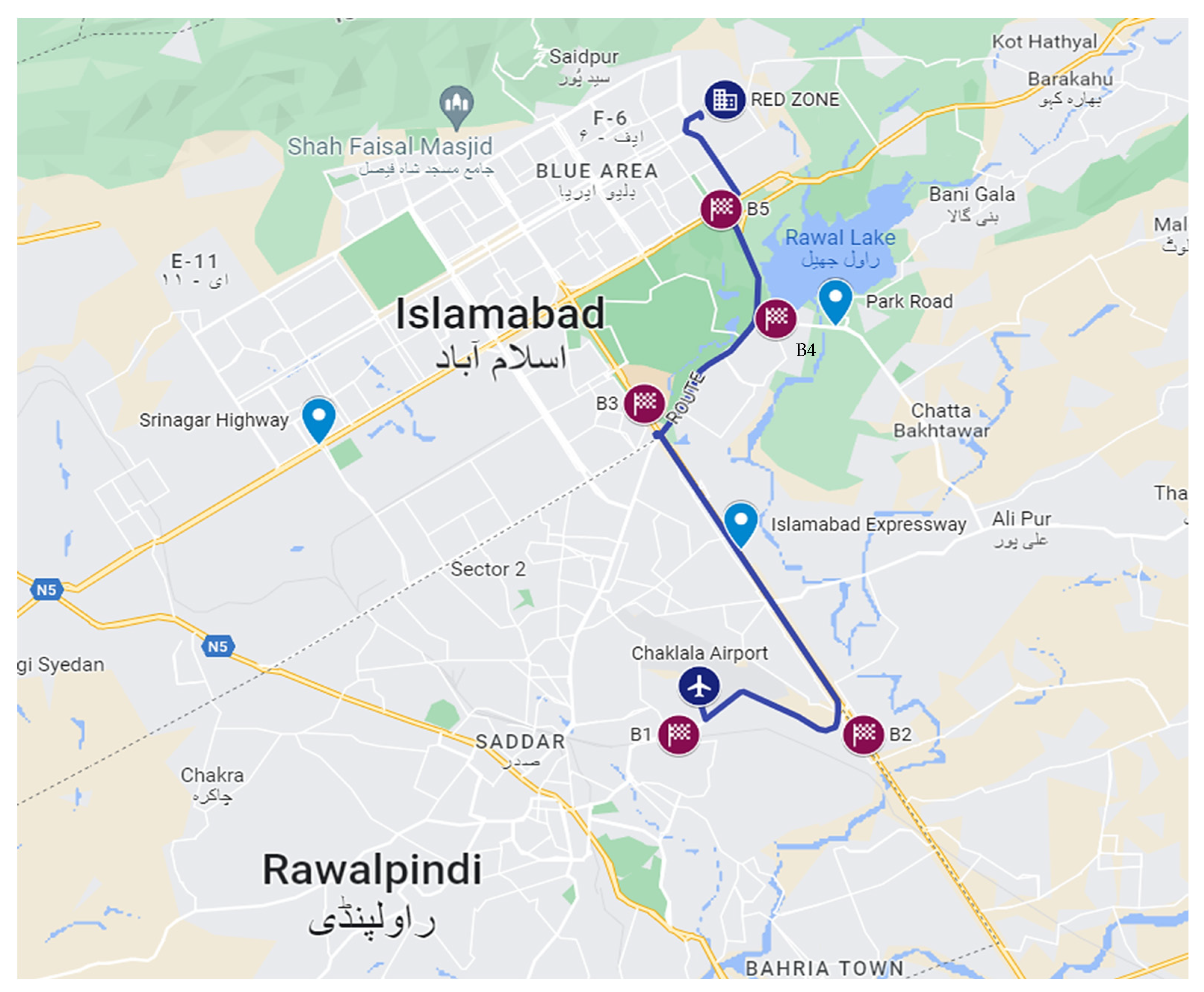
Figure 1. Route choice for VIP movements with major blockades (Source: Google Maps).
Sustainability 16 05278 g001
Figure 2. Methodology framework.
Sustainability 16 05278 g002
Figure 3. VISSIM v7 Model—Airport Rd.
Sustainability 16 05278 g003
Figure 4. VISSIM v7 Model—Kural Rd.
Sustainability 16 05278 g004
Figure 5. VISSIM v7 Model—Fizabad Rd.
Sustainability 16 05278 g005
Figure 6. VISSIM v7 Model—Park Rd.
Sustainability 16 05278 g006
Figure 7. VISSIM v7 Model—Serena Intersection.
Sustainability 16 05278 g007
Figure 8. Queue length (freeway segments).
Sustainability 16 05278 g008
Figure 9. Delay (freeway segments).
Sustainability 16 05278 g009
Figure 10. Queue length (signalized intersection).
Sustainability 16 05278 g010
Figure 11. Delay (signalized intersection).
Sustainability 16 05278 g011
Figure 12. Travel time delay costs all locations in USD/h.
Sustainability 16 05278 g012
Figure 13. Increment in total delay cost concerning blockade time.
Sustainability 16 05278 g013
Figure 14. Existing emission level at all locations (g/h).
Sustainability 16 05278 g014
Figure 15. CO emissions of all variants (g/h).
Sustainability 16 05278 g015
Figure 16. NOx emissions of all variants (g/h).
Sustainability 16 05278 g016
Figure 17. VOC emissions of all variants (g/h).
Sustainability 16 05278 g017
Table 1. Key demographics of survey participants.
VariableSample % AgeVariableSample % Age
Gender Cities
Male85%Islamabad62%
Female15%Rawalpindi38%
Age Vehicle Ownership
<2041%Bike31%
20–3053%Car27%
30–404%Both21%
40 above2%Donot own a vehicle21%
Income Daily mode of Travel
<20k PKR (below 90 USD)55%Car 42%
20k–40k PKR (90–179 USD)23%Bike36%
40k–60k PKR (179–269 USD)10%Public Transport22%
>60k PKR (above 269 USD)12%
Employment Trip Purpose
Govt./private Employee23%Business21%
Unemployed/Student56%Education59%
Self-employed/Business21%Work20%
Table 2. Traffic volume freeway segments.
LocationVolumeCompositionPeak HourSpeed Limit
(km/h)
MotorcyclesCars/JeepsH.V
Airport Road37010.400.590.018:00–9:0070
Kural45790.350.560.098:30–9:3080
Faizabad57250.420.540.045:15–6:1580
Park Road28210.390.580.038:00–9:0060
Table 3. Traffic volume, Serena Intersection.
MovementEBWBNBSB
Volume2935531965932418
Table 4. MNL model formulation with likelihood ratio tests.
S. No (i)ModelLog-LikelihoodLL Ratio Test ValueDegree of Freedom AddedLikelihood p Value
1Base model (general β for travel time and travel cost)−1554.12---
2β time distributed for each choice−1554.030.1820.91 **
3General β for gender introduced−1529.3949.4612.03 × 10−12 *
4β gender distributed for each choice−1456.5145.7811.45 × 10−33 *
5β for high income category introduced−1452.537.9410.004835 *
6β for young age category introduced−1452.53011 **
* Indicates the results that are statistically significant at a 99% confidence interval, leading to the rejection of the null hypothesis. Therefore, model i + 1 is preferred over model i. ** Indicates the test results that are not statistically significant at a 90% confidence interval.
Table 5. Model estimations.
EstimateStd. Err.t-Ratio (0)Rob. Std. Err.Rob. t-Ratio (0)
asc_car0NA ***NA ***NA ***NA ***
asc_bike−0.317970.2105398−1.5102763630.1593545−1.99 *
asc_van−1.879310.22901849−8.2059157170.2102371−8.93 *
b_tt−-0.01880.01105408−1.7009012580.0066334−2.83 *
b_cost−0.002850.00120364−2.3657874930.0007567−3.76 *
b_female_car0NA ***NA ***NA ***NA ***
b_female_bike−2.558270.2846348−8.9878962040.358116−7.14 *
b_female_van0.6309190.178412383.5362944590.30204742.08 *
b_high_income0.4593430.163840992.8035930860.26810921.71 **
LL(start):−1762.17
LL(final):−1452.53
Adj. Rho-squared:0.0628
AIC:2919.06
* Significant at 99% confidence interval. ** Significant at 95% confidence interval. *** NA stands for Not Applicable.
Table 6. Value of travel time (VOTT).
ExpressionValue (PKR)Value (USD)Robust s.e.Rob.t-Ratio (0)
VOTT (per min)6.60290.0292.17723.03
VOTT (per hour)396.1741.77130.63493.03
Note: PKR stands for Paksitani Rupee.
Table 7. Fuel consumption cost for different scenario runs.
Blockade Time (min)Total Fuel Consumed (L/h)Fuel CostFuel Consumption Cost
(PKR/L)(USD/L)(PKR/h)(USD/h)
04872641.184128,568577
26162641.184162,624729
49912641.184261,6241173
612382641.184326,8321466
815522641.184409,7281837
Table 8. Total delay cost for each scenario run.
Blockade TimeTotal TTDCFuel Consumption CostTotal Delay Cost
(PKR/h)(USD/h)(PKR/h)(USD/h)(PKR/h)(USD/h)
067,569303128,568577196,137880
2100,350450162,624729262,9741179
4191,334858261,6241173452,9582031
6361,0371619326,8321466687,8693085
8614,5882756409,72818371,024,3164593
Disclaimer/Publisher’s Note: The statements, opinions and data contained in all publications are solely those of the individual author(s) and contributor(s) and not of MDPI and/or the editor(s). MDPI and/or the editor(s) disclaim responsibility for any injury to people or property resulting from any ideas, methods, instructions or products referred to in the content.