Ultimate Pit Limit Optimization Method with Integrated Consideration of Ecological Cost, Slope Safety and Benefits: A Case Study of Heishan Open Pit Coal Mine

Abstract

The ecological impacts of mining and the instability of slopes are the key factors restricting the safe, efficient, and low-carbon production of open-pit mines. This study focused on the ultimate pit limit (UPL) optimization under the concept of sustainability by integrating consideration of the economic benefit, ecological impact, and slope geometry. The integrated UPL optimization model based on the floating cone method was proposed by establishing a quantitative model for ecological impacts arising from open-pit coal mining in arid or semi-arid weak ecological land and a cost calculation model of slope reinforcement based on the Monte Carlo method. The case study revealed that steepening the slope angle of given regions resulted in random variations in the quantity of ore rock and the limit morphology. There was an average economic profit rise of USD 9.54M with every 1° increase in slope angle, but the probability of slope instability and the reinforcement cost grows exponentially. In the arid or semi-arid weak ecological land, the ecological costs exceeded 20% of the mines’ average pure economic gains. The proposed optimization method contributes to obtaining an integrated optimal UPL, improving the benefits and the ore recovery rate.

1. Introduction

Sustainable development (SD) concepts have been integrated into mining design for more than 30 years. In the initial stage, strategic research integrated these concepts within the mining industry [1,2,3,4]. Subsequently, researchers devised framework systems of SD indicators to quantitatively guide the design and production in mining [5,6]. Adibi et al. proposed a quantitative method that integrated SD factors into the ultimate pit limit (UPL) design, transforming UPL optimization into a multiple-attribute decision-making problem and solving it using the similarity to the ideal solution method [7]. This seminal study facilitated a deeper integration of SD within the mining industry. However, this method predominantly focused on weight distribution, which somewhat constrained its ability to holistically and objectively account for economic, environmental, safety, and other considerations. While several subsequent quantitative studies have explored the impact of mining activities on SD [8,9,10,11,12], their practical application to mining design remains limited.

Previous research identified five dimensions of sustainable mining practices: economy, environment, community, safety, and efficiency [13,14]. However, integrating these factors as internal parameters within the mining industry proves challenging. These factors are not only difficult to quantify but also interact with each other, which can lead to potential conflicts during the optimization process, resulting in failures. The author has been committed to developing quantitative mining optimization models to integrate by considering these factors as cost parameters. In past studies, the author proposed several algorithms to integrate by considering both economic and environmental factors in mining design [15,16,17]. Building on this foundation, the present study further refines the ecological cost quantitative model based on the environmental conditions around a coal mine and introduces safety as an additional SD factor in the UPL optimization algorithm.

The ecological impact of mining activities is influenced by various factors. Numerous studies on the ecological issues of mining seek to develop a system for environmental evaluation indicators [18,19,20]. These evaluation models primarily aim to quantify the environmental harm caused by mining. To further determine the impact of mining on the ecological environment, the concept of ecological cost, which traces back to the Principles of Economics proposed by Marshall [21], was proposed to evaluate the environmental issues of open pit mines. This concept correlates the economic and ecological benefits by considering the external costs consumed in the production process as ecological costs. Ugochukwu et al. developed a health-risk-based pollution economic costing model that considered heavy metal pollution in surface and ground water, as well as soil, to evaluate the health and environmental costs caused by mining activities [22]. Meanwhile, Badakhshan et al. assessed the ecological cost of a mine using a framework-based approach, factoring in the human development index, mining scale, location of the mine, mining method, type of mineral, and environmental and ecosystem sensitivities [23]. However, the primary application of these models is for ecological reclamation rather than mining design. Badiozamani and Askari-Nasab proposed an integrated long-term mine planning model that considered the tailings model, the reclamation plan, and the waste management within a single framework [24]. Furthermore, the author has quantified the ecological harm in mining regions based on the ecological footprint theory and the energy consumption intensity. An ecological cost model was established that internalized environment factors as costs within the economic benefit of UPLs, and thereby effectively integrated the concept of SD into the mining design [16].

In terms of safety, the slope stability of open-pit mines is particularly important. As a primary parameter of UPL, the slope angle affects the geometry of the mine and the quantity of stripping, as well as the production safety and the area of land degradation [25]. Slackening the slope angle increases the stripping ratio, subsequently exacerbating environmental impacts. Conversely, steepening the slope angle reduces the mining cost but heightens the risk of landslides [26,27]. Numerous previous studies have aimed to establish calculation approaches for evaluating pit slope stability [28,29,30,31,32,33,34,35,36]. However, integrating these noteworthy achievements into UPL optimization design remains challenging due to the ambiguous relationship between landslide risk and mining benefits. Recent studies on UPL optimization [37,38,39,40] frequently underscore the characteristics of slope angle, which directly reflects land degradation, carbon emissions, and waste amount, with minimal focus on its environmental impacts.

The instability of high and steep slopes and the ecological impacts caused by mining are the key factors restricting the pursuit of safe, high-efficiency, and low-carbon mining production. Factors such as profitability, slope stability, and ecological impacts of open-pit mining intensify the intricacy of the UPL optimization process when synergistically considered. To assimilate the SD factors of environment and safety into UPL optimization, this study introduces a refined UPL optimization method tailored for open-pit coal mines. The study was delineated over three phases. The first stage involved developing an ecological cost model, specifically for arid or semi-arid mining of weak ecological lands, to precisely evaluate the environmental impacts caused by mining activities in the Heishan open-pit coal mine. The second phase was mainly focused on the formulation of a safety cost model to elucidate the correlation between the geometric parameters of slope and associated costs. The final step was to integrate the ecological and safety cost models into the UPL optimization model based on the floating cone method. The results from this study are pivotal in advancing sustainable, low-carbon, safe, and efficient mining in open-pit mines.

2. Methods

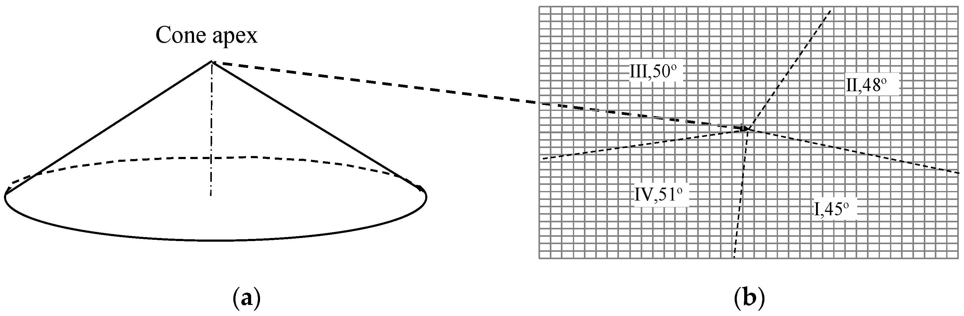
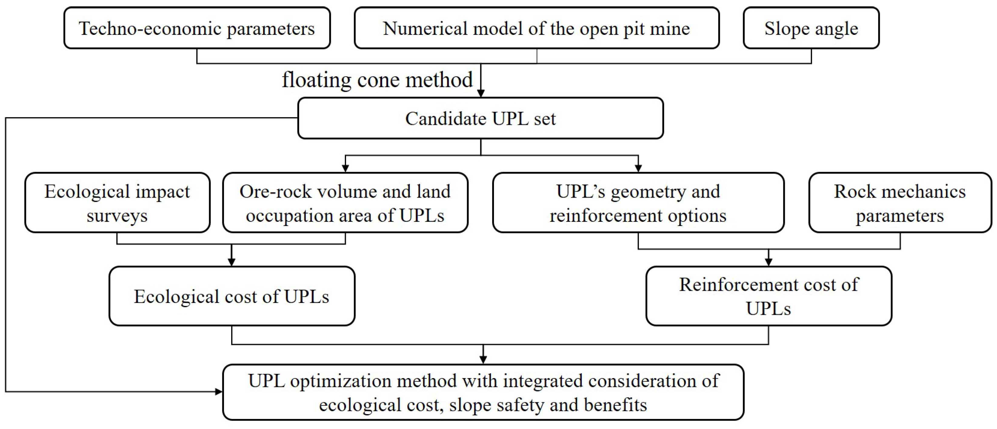
2.1. UPL Optimization Using Floating Cone Method

The UPL design can be formulated using several theoretical methods, such as the floating cone method [41,42], a type of quasi-optimization method, and other mathematical methods like the Lerchs–Grossmann graph theory method. Due to the anisotropic characteristics of open-pit slopes on lithologic joints and fissures, distinct slope angles are observed for different directions and depths. The inclination of the cone can be adjusted based on the parameters of direction and depth (see Figure 1). A more realistic solution within the accepting error will be obtained. Thus, the UPL optimization of the open-pit mine involved in this paper is carried out based on the floating cone method. The previous works by the author have delineated the theoretical and calculative methods for UPL optimization [16,17].

2.2. Ecological Cost Model of Open-Pit Coal Mine in Arid or Semi-Arid Weak Ecological Land

Open-pit coal mining results in expansive pits occupying vast land areas, with the stripped waste rocks further demanding substantial storage space. Such mining activity disables the biomass production capability of the land and removes the plants in diggings, thereby disrupting ecosystem functions. Drawing inspiration from previous studies, primarily focused on the thermo-ecological cost of hard coal [43], this study presents an ecological cost model encompassing the entire mining cycle of open-pit coal mines.

2.2.1. Evaluation Method of Occupied and Damaged Area Caused by Mining

The occupied and damaged area caused by mining can be divided into three categories, including the surface area of the open-pit mine ($A_m(\Phi )$, hm²), the area occupied by ancillary facilities ($A_o$, hm²), and the area taken up by waste stones and tailings ($A_w(\Phi )$, hm²). Here, $\Phi ({\phi }_1,{\phi }_2,{\phi }_3,\cdot \cdot \cdot ,{\phi }_n)$ represents a finite set of slope angles in various directions within the UPL. ${\phi }_n$ denotes the slope angle in the n-th direction. $A_m(\Phi )$ is determined by the UPL design. $A_o$ is regarded as a constant obtained from blueprints. $A_w(\Phi )$ can be calculated as follows:

$$A_w(\Phi )=Q_w(\Phi )\frac{{\gamma }_w}{10000H_w}{S}_w$$

(1)

where $Q_w(\Phi )$ is the volume of waste rocks in the optimized UPL based on the slope angle set (m³), ${\gamma }_w$ is the expansion coefficient of the stacked waste rock, $H_w$ is the height of the waste rock field (m), and $S_w$ is the morphology coefficient of the waste rock field.

2.2.2. Direct Economic Loss

Mining activities can result in land degradation, impeding the capacity of land for biomass production. Compensation for land expropriated for mining typically reflects the combined economic value. Thus, the direct economic loss ($C_z(\Phi )$, USD) can be calculated based on the land expropriated price and the total area of land occupation, expressed as:

$$C_z(\Phi )=c_z(A_m(\Phi )+A_w(\Phi )+A_o)$$

(2)

where $c_z$ is the land expropriation price (USD/hm²).

2.2.3. Exogenous Ecological Value Loss

The concept of exogenous ecological value loss serves to evaluate the damage to the ecosystem and the land degradation of ecological functions due to surface vegetation destruction during mining activities. This study proposes a new calculation model, which focuses on arid or semi-arid weak ecological land based on the previous study [17]. The service functions provided by grassland ecosystems mainly contain water conservation, soil conservation, carbon sequestration, biodiversity maintenance, grassland recreation, oxygen release, air purification, and nutrient cycling.

The value of water conservation ($V_{(g{H}_{2}O)}(\Phi )$, USD/a) can be calculated by Formula (3):

$$V_{(g{H}_{2}O)}(\Phi )={\displaystyle {\sum }_{i=1}^{F}10JKR}(C_{(H_{2}O)}+L)A_i(\Phi )$$

(3)

where $F$ is the number of grassland types occupied by the mining activities, $A_i(\Phi )$ is the area of grassland type i (hm²), $J$ is the average rainfall in mining area (mm/a), $K$ is the proportion of runoff rainfall to the total rainfall volume in the mining area, $R$ is the runoff reduction coefficient comparing grassland to bare land, $C_{(H_{2}O)}$ is the unit price of the water resource (USD/m³), and $L$ is the cost of water purification (USD/m³).

The value of soil conservation ($V_{gs}(\Phi )$, USD/a) can be calculated by Formula (4):

$$V_{gs}(\Phi )={\displaystyle {\sum }_{i=1}^F{\displaystyle {\sum }_{j=1}^4(\frac{A_i(\Phi )M_i{P}_1}{\rho }+\frac{A_i(\Phi )M_i{R}_l{P}_2}{\rho }+\frac{A_i(\Phi )M_i{E}_j{P}_{3j}}{r_j})}}$$

(4)

where $M_i$ is the soil conservation capacity of class n grassland (unit: hm²·a); $\rho$ is the soil bulk density (t/m³); $R_l$ is the proportion of sediment deposition in reservoirs, rivers and lakes due to soil erosion (commonly set to 0.24); $E_j$ is the content of specific elements in the soil, such as nitrogen (when j = 1), phosphorus (when j = 2), potassium (when j = 3), and organic matter(when j = 4) (%); $r_j$ is the content of nitrogen, phosphorus, potassium, and organic matter in the fertilizer and organic matter (%); $P_1$ is the cost incurred for the excavation of per unit volume of soil (USD/m³); $P_2$ is the cost of unit capacity (USD/m³), and $P_{3j}$ is the prevailing market price of fertilizer and organic matter (USD/t).

The value of carbon sequestration can be categorized into two main segments: plant-based and soil-based carbon sequestration. The values of plant-based ($V_{gC1}(\Phi )$, USD/a) and soil-based carbon sequestration ($V_{gC2}(\Phi )$, USD/a) can be calculated using Formulas (5) and (6), respectively.

$$V_{gC1}(\Phi )={\displaystyle {\sum }_{i=1}^F{\phi }_{C{O}_2}}{q}_i c_{C{O}_2}{A}_i(\Phi )$$

(5)

$$V_{gC2}(\Phi )={\displaystyle {\sum }_{i=1}^{F}10\rho h\left[D_{SOC}+D_{SIC}(1+{\epsilon }_{st})\right]{\tau }_C{c}_{C{O}_2}}{A}_i(\Phi )$$

(6)

where ${\phi }_{C{O}_2}$ is the coefficient of carbon sequestration (commonly set to 1.62), $q_i$ is the net primary productivity of grassland type i (t/hm²·a), $c_{C{O}_2}$ is the cost of carbon sequestration (USD/t), $h$ is the average soil depth of the grassland (m), $D_{SOC}$ is the organic carbon density in the soil (g/kg), $D_{SIC}$ is the inorganic carbon density in the soil (g/kg), ${\epsilon }_{st}$ is the migration rate of soil pollutants (%), and ${\tau }_C$ is the conversion coefficient transforming carbon to carbon dioxide (with a standard value of 3.6667).

The economic value of biodiversity maintenance ($V_{gb}(\Phi )$, USD/a) can be calculated by Formula (7):

$$V_{gb}(\Phi )={\displaystyle {\sum }_{i=1}^F{S}_{bi}}{A}_i(\Phi )$$

(7)

where $S_{bi}$ is the annual species loss opportunity cost per unit area of grassland type i (t/hm²·a), determined by the Shannon Wiener diversity index (see

Table 1. Shannon Wiener diversity index.

Shannon Wiener Index	(0, 1)	[1, 2)	[2, 3)	[3, 4)	[4, 5)	[5, 6)	[6, +)
Sb (USD·hm−2·a−1)	435	725	1450	2900	4350	5800	7250

).

The value of grassland recreation ($V_{gr}(\Phi )$, USD/a) is calculated from Formula (8):

$$V_{gr}(\Phi )={\displaystyle {\sum }_{i=1}^F{c}_{gi}}{A}_i(\Phi )$$

(8)

where $c_{gi}$ is the unit grassland recreation value (USD/(hm²·a)).

The value of oxygen release ($V_{g{O}_2}(\Phi )$, USD/a) can be calculated using Formula (9):

$$V_{g{O}_2}(\Phi )={\displaystyle {\sum }_{i=1}^F{\varphi }_{O_2}{q}_i{C}_{O_2}}{A}_i(\Phi )$$

(9)

where ${\varphi }_{O_2}$ is the coefficient for oxygen release (commonly set to 1.19 based on the photosynthesis reaction), $C_{O_2}$ is the cost of oxygen production (USD/t).

The value of air purification ($V_{ga}(\Phi )$, unit: USD/a) can be calculated using Formula (10):

$$V_{ga}(\Phi )={\displaystyle {\sum }_{i=1}^F(Y_{iS{O}_2}{C}_{S{O}_2}+Y_{iD}{C}_D)}{A}_i(\Phi )$$

(10)

where $Y_{iS{O}_2}$ is the sulfur dioxide absorption capacity for grassland type i (t/hm²·a), $Y_{iD}$ is the dust-retention capability for grassland type i (t/hm²·a), $C_{S{O}_2}$ is the treatment cost for sulfur dioxide (USD/t), and $C_D$ is the treatment cost for dustfall (USD/t).

The value of nutrient (nitrogen and phosphorus) accumulation ($V_{gNP}(\Phi )$, USD/a) can be calculated using Formula (11):

$$V_{gNP}(\Phi )={\displaystyle {\sum }_{i=1}^F(k_{Ni}{p}_N+k_{Pi}\beta p_P)q_i}{A}_i(\Phi )$$

(11)

where $k_{Ni}$ and $k_{Pi}$ are the proportions of nitrogen and phosphorus content in the net primary productivity of grassland type i (t/hm²·a), respectively, $\beta$ is the transfer coefficient from phosphorus to P₂O₅ (commonly set to 2.2903), $p_N$ and $p_P$ are the prices of nitrogen fertilizer and phosphorus fertilizer (P₂O₅), respectively (USD/t).

The exogenous ecological value loss ($V_{gall}(\Phi )$, USD/a) is the sum of these eight items:

$$\begin{array}{c}{V}_{gall}(\Phi )=V_{(g{H}_{2}O)}(\Phi )+V_{gs}(\Phi )+V_{gC1}(\Phi )+V_{gC2}(\Phi )+V_{gb}(\Phi )\\ +V_{gr}(\Phi )+V_{g{O}_2}(\Phi )+V_{ga}(\Phi )+V_{gNP}(\Phi )\end{array}$$

(12)

2.2.4. Treatment Cost of Environmental Pollution

The treatment cost of environmental pollution covers all costs relating to environmental conservation, excluding those related to ecological reclamation. These costs contain the treatment of water pollution, air pollution, solid waste, and soil pollution.

Focusing on water pollution, its treatment cost is divided into two categories, including the production and household sewage and the pollution of shallow groundwater caused by harmful elements from coal gangue yards or mining fields with rainfall into the soil. The treatment cost of production and household sewage ($V_{W1}(\Phi )$, USD/a) can be calculated using the following formula:

$$V_{W1}(\Phi )=c_{w1}\left[q_w(\Phi )+q_o(\Phi )\right]e_{wt}$$

(13)

where $c_{w1}$ is the treatment fee of per unit volume sewage (USD/m³), $q_w(\Phi )$ is the annual ore extraction quantity (t/a), $q_o(\Phi )$ is the annual rock extraction quantity (t/a), $e_{wt}$ is the sewage discharge stemming from both production processes and domestic water consumption of per unit extraction (m³/t).

The treatment cost of polluted shallow groundwater can be evaluated using Formula (14):

$$V_{W2}(\Phi )=10a\lambda J{c}_{w2}{A_t}^{″}(\Phi )$$

(14)

where $a$ is the adjustment coefficient (a constant coefficient influenced by polluted surface water environment, the multiples of supernational discharge standards for water pollutants, and the location of discharge, commonly set to 2.625), $\lambda$ is the infiltration coefficient of soil (commonly set to 0.12), $J$ is the annual mean rainfall in the mining vicinity (unit: mm/a), $c_{w2}$ is the unit treatment cost of leaching water (USD/m³), ${A_t}^{″}(\Phi )$ is the occupied area of the mining pit and waste in the year t (commonly equated to the area of UPL and waste dump site, hm²/a).

The treatment cost of soil pollution ($C_{ST}(\Phi )$, USD/a) can be calculated using Formula (15):

$$C_{ST}(\Phi )=c_{ST}\frac{\left[A_m(\Phi )+A_w+A_o\right](1+{\epsilon }_{st})}{T(\Phi )}$$

(15)

where $c_{ST}$ is the price of soil remediation per unit volume (USD/hm²), ${\epsilon }_{st}$ is the pollutant migration rate originating from mining (%), and $T(\Phi )$ is the duration of UPL operation with a slope angle of $\Phi$ (a).

The treatment cost of solid waste ($C_{SW}(\Phi )$, USD/a) can be evaluated using Formula (16):

$$C_{SW}(\Phi )={\displaystyle {\sum }_{i=1}^5\frac{1}{1000}{c}_{swi}\left[q_w(\Phi )+q_o(\Phi )\right]e_{swi}}$$

(16)

where $c_{swi}$ is the unit cost for treating the i-th type of solid waste (i = 1 for coal gangue, i = 2 for hazardous solid waste, i = 3 for fly ash, i = 4 for slags, i = 5 for other solid wastes) (USD/t), $e_{swi}$ is the emission quantities of the i-th solid waste type from per unit stripping (kg/t).

The air contaminants from open-pit coal mines predominantly contain coal-burning byproducts and dust. Coal-burning pollution is mainly caused by SO₂, NO_X, and fume dust, whereas dust pollution is related to the fee of watering volume. Thus, the treatment costs of air pollution ($C_a(\Phi )$, USD/a) can be calculated using Formula (17):

$$C_a(\Phi )={\displaystyle {\sum }_{i=1}^3{c}_{ai}\left[q_w(\Phi )+q_o(\Phi )\right]e_{ai}}+\frac{n_d{x}_w{A}_{nd}(\Phi )V_a{C}_{H_{2}O}}{1000}$$

(17)

where $c_{ai}$ is the treatment cost for specific pollutants (i = 1 for SO₂, i = 2 for NO_X, i = 3 for fume dust) (USD/t), $e_{ai}$ is the emission amount of SO₂, NO_X, and fume dust per unit stripping volume (kg/t), $n_d$ is the number of production days per year (d/a), $x_w$ is the daily watering frequency (n/d), $A_{nd}(\Phi )$ is the watering area during each instance per day (m²/n/d), $V_a$ is the watering volume used per unit area (m³/m²), and $C_{H_{2}O}$ is the prevailing water price in the mining community (USD/m³).

The comprehensive cost for environmental treatment is the cumulative sum of the aforementioned components, as represented by:

$$C_{wall}(\Phi )=V_{W1}(\Phi )+V_{W2}(\Phi )+C_{ST}(\Phi )+C_{SW}(\Phi )+C_a(\Phi )$$

(18)

2.2.5. Ecological Cost of Energy Consumption

The mining production process heavily relies on fossil fuels, such as diesel, petrol, and coal, leading to significant greenhouse gas emissions. An ecological cost model for energy consumption ($C_C(\Phi )$, USD/a) has been formulated considering emission characteristics of different energy consumption as well as the carbon trading market, carbon capture cost, and carbon tax as follows:

$$C_C(\Phi )=(q_o(\Phi )+q_w(\Phi ))(\frac{e_e{r}_e{e}_c{\eta }_c}{1000}+{\displaystyle {\sum }_{i=1}^o\frac{e_{hi}{\eta }_{hi}}{1000}}){\tau }_C{C}_{C{O}_2}$$

(19)

where $e_e$ is the electricity consumption per unit mining stripping (kWh/t), $r_e$ is the proportion of thermal power generation to total power generation, $e_c$ is the standard coal consumption per kilowatt hour (kg/kWh), ${\eta }_c$ is the carbon emission coefficient of standard coal, $o$ is the category of primary fossil energy consumed, $e_{hi}$ is the consumption of the i-th type of primary fossil energy per unit of mining stripping (kg/t), ${\eta }_{hi}$ is the carbon emission coefficient of the i-th type of primary fossil energy (i = 1 for diesel, i = 2 for petrol), ${\tau }_C$ is the conversion coefficient transforming carbon to carbon dioxide (commonly set to 3.6667), and $C_{C{O}_2}$ is the cost of carbon capture and sequestration (USD/t).

2.2.6. Reclamation Cost

The reconstructions of soil, water, and vegetation are the primary aims for the open-pit coal mine ecological reclamation in arid or semi-arid weak ecological land. Water scarcity and weak ecological systems are the main limiting factors in arid or semi-arid land, which increase the cost of mine ecological reclamation. The reclamation cost ($C_{rt}(\Phi )$, USD) for year t of mining can be calculated as follows:

$$C_{rt}(\Phi )=a_t(\Phi )c_r$$

(20)

where $a_t$ is the ecological reclamation area in year t (hm²), $c_r$ is the cost of reclaiming or conserving per unit area of land (USD/hm²).

2.3. Safety Cost Calculation Model of Open Pit Mine Slope

The slope angle is usually steepened to reduce the amount of rock stripping, which decreases the rock stripping cost, thereby improving the overall economic efficiency of mining. The general approach is to contract the pithead while fixing the pit bottom to achieve this goal [26]. However, these individual optimization methods have several limitations. First, the optimal slope angle, which balances between slope stability and benefits, remains unidentified. Second, the steepening of the slope angle is more associated with the benefits and resource utilization rate derived from the quantity of stripped ore or rock quantity rather than a designated change that locks the pit bottom [27]. Third, the adjustment of the slope angle should factor in ecological impacts. Such changes not only affect the quantity of stripped ore or rock and the mining range but also lead to variations in ecological impacts and carbon emissions [44,45].

2.3.1. Reliability Analysis of Open-Pit Coal Mine Slope

Reliability analysis, which employs parameters such as rock properties, geometrical characteristics, groundwater, and various impacts, is widely used to calculate the reliability index or failure probability. This method offers a quantitative description of slope stability [46,47,48]. In this study, the Geostudio software (Slope/W) was utilized to analyze the reliability of slopes with different UPL geometric parameters (slope angle and height) based on the Monte Carlo (MC) simulation method.

The limit state equation of slope is determined by the Bishop method:

$$G(W,c,u,\phi )={\displaystyle \sum _{i=1}^N[c_i\Delta x_i+\Delta W_i(1-r_u)\tan {\phi }_i]/[\cos {\alpha }_i(1+\tan {\alpha }_i\tan {\phi }_i)]-{\displaystyle \sum _{i=1}^N\Delta W\sin {\phi }_i}}$$

(21)

where $c$ is the effective cohesion (kPa), $\Delta W$ is the weight of soil stripe (kN), $u$ is the pore water pressure (kPa), $\phi$ is the effective internal friction angle (°), $r_u$ is the pore water pressure coefficient.

The instability probability of the slope is calculated by Formula (22):

$$P_f=P(G<0)={\displaystyle {\int }_{-\infty }^{0}f(G)}dz={\displaystyle {\int }_{-\infty }^{1}F(X_1,X_2,X_3,\dots ,X_n)}df$$

(22)

Table 2. Acceptable instability probability index of open-pit mine slopes.

Open Pit Mine Slope	Instability Probability	Reliability Index
Most geotechnical engineering	≤0.1%	3.1
Normal open-pit mine slope	≤0.01%	3.7
Rock open-pit mine slope	0.3%	2.86
An open-pit mine slope in Peru	≤0.3%	2.8
Dabaoshan open-pit iron mine slope	0.084%	3.14
Qianyanshan open-pit iron mine slope	0.004%~0.105%	3.08~4.45
Jianshan open-pit mine slope	0.3%~1%	2.8~2.3
Yima open-pit coal mine slope	≤0.05%	3.29
Yamansu open-pit iron mine slope	0.037%~0.292%	2.76~3.38

illustrates that the typically acceptable instability probability ranges between 0.01% and 0.3%. In contrast, based on current engineering expertise, the reliability index lies between 3.7 and 2.8 [49]. When designing large surface mines aimed at long-term operations, the paramount consideration is the overall slope stability. Thus, the slope safety level should be designated as grade I, suggesting that a relatively higher reliability index value should be adopted.

2.3.2. Reinforcement Cost of Open-Pit Coal Mine Slope

The reliability index serves as a criterion to determine the need for reinforcement measures, thereby enabling the calculation of reinforcement costs for open-pit coal mine slopes. Large-scale integral sliding of a rock mass along the structural plane is a catastrophic accident for a large open-pit mine. For large-scale slope deformation, light reinforcement techniques are often inadequate in enhancing the anti-slide capability of unstable rock masses. Conversely, heavy reinforcement approaches, such as retaining walls or anti-slide piles, are constrained by the limited construction space available on open-pit mine slopes. The reinforcement design of mine slopes often depends on the failure mode and scale. Additionally, the change of slope angle caused by the UPL optimization results also affects the selection of reinforcement techniques. The reinforcement cost ($C_f(\Phi )$, USD) associated with varying slope angles can be calculated using Formula (23):

$$C_f(\Phi )={\displaystyle {\sum }_i^m{B}_i\left[I(\Phi ),S(\Phi ),M(\Phi )\right]}{P}_i(\Phi )$$

(23)

where $m$ is the count of sub-project categories within the reinforced engineering, $B_i\left[I(\Phi ),S(\Phi ),M(\Phi )\right]$ is the engineering tasks of the i-th sub-project (m²), $I(\Phi )$ represents the reinforcement method adopted, $S(\Phi )$ is the reinforcement range of slope (m²), $M(\Phi )$ is the type of reinforcement material used, and $P_i(\Phi )$ is the comprehensive price per unit engineering task of the i-th sub-project contained labor costs, material costs, machinery costs, business management fees, regular fees, profits, and taxes (USD/m²).

2.4. UPL Optimization Model with Integrated Consideration of Ecological Cost, Slope Safety, and Benefits

The framework of the UPL optimization model with integrated consideration of ecological cost, slope safety, and benefits is shown in Figure 2.

The result of UPL optimization based on the floating cone method produces a sequence of limits with different slope angles. Excluding the impacts of slope stability and ecological environment, the economic benefits ($C_M(\Phi )$, USD) associated with different slope angles can be calculated using Formula (24):

$$C_M(\Phi )=V_c(\Phi )(P_c-C_c)-V_r(\Phi )C_r$$

(24)

where $V_c(\Phi )$ is the quantity of coal mined in the UPL with a slope angle of $\phi$(t), $V_r(\Phi )$ is the volume of rock stripped in the UPL with a slope angle of $\phi$ (m³), $P_c$ is the price of raw coal (USD/t), $C_c$ is the unit mining cost (USD/t), and $C_r$ is the unit rock stripping cost (USD/m³).

During the whole cycle of mining, the cumulative ecological cost ($C_S(\Phi )$, USD) can be calculated based on the proposed models in Section 2.2 as follows:

$$C_S(\Phi )=C_Z(\Phi )+V_{gall}(\Phi )[T(\Phi )+n_t]+C_{wall}(\Phi )T(\Phi )+C_c(\Phi )+C_{rt}(\Phi )$$

(25)

where $T(\Phi )$ is the production life in the UPL with a given slope angle of $\phi$(a), $n_t$ is the duration required for the ecological environment to be restored to the pre-mining state (a).

The reinforcement will only focus on the unstable slopes that exhibit instability probabilities surpassing the acceptable probability. The reinforcement cost can be calculated using Formula (26):

$$C_J(\Phi )=\{\begin{array}{ll}0& (P_f(\Phi )\le \overline{P})\\ {\displaystyle {\sum }_{i=1}^n{C}_f(\Phi )}& (P_f(\Phi )>\overline{P})\end{array}$$

(26)

where $n$ is the total number of slopes requiring reinforcement.

Therefore, the comprehensive economic benefit ($W(\Phi )$, USD) for the UPL, which integrated considerations of ecological environment, slope safety, and mining benefit, can be calculated as:

$$W(\Phi )=C_M(\Phi )-C_S(\Phi )-C_J(\Phi )$$

(27)

3. Case Study

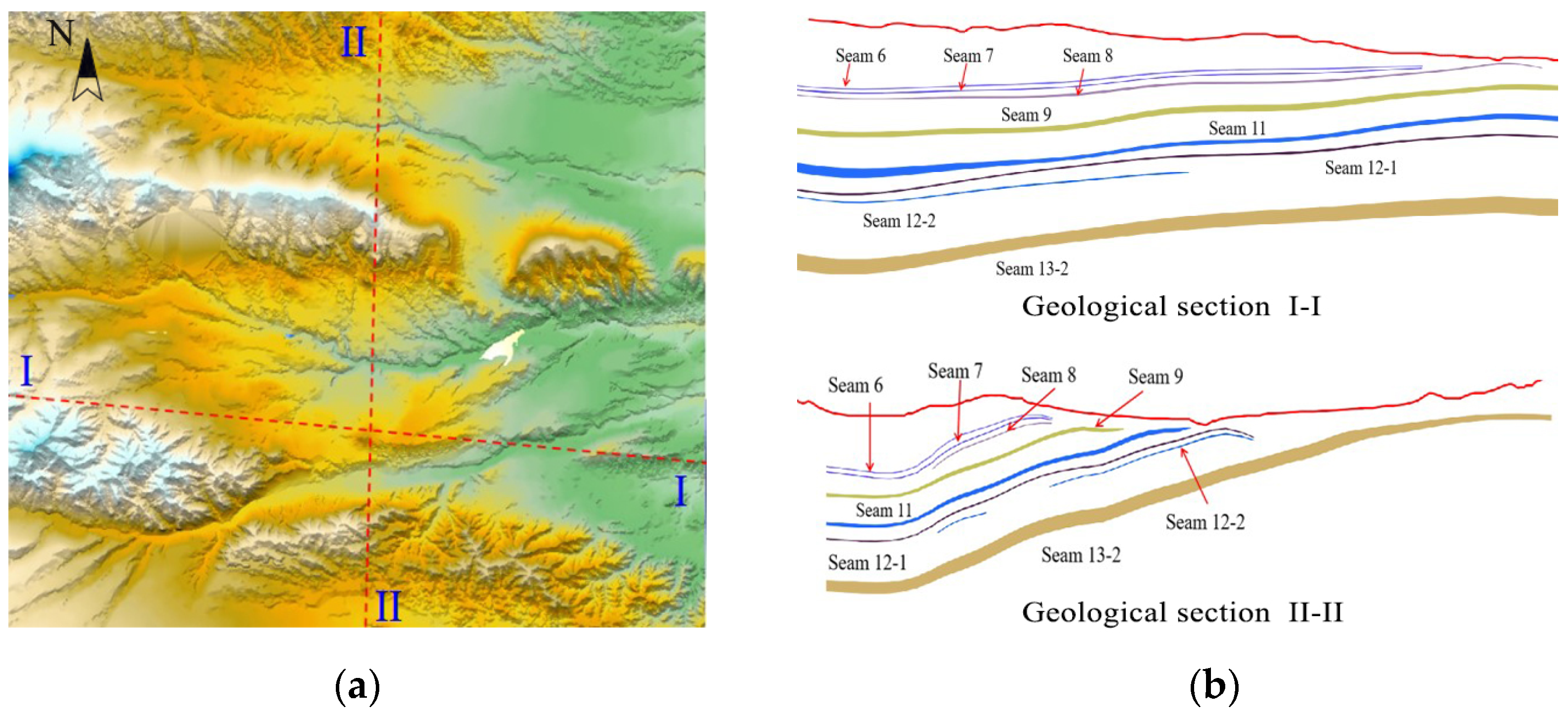
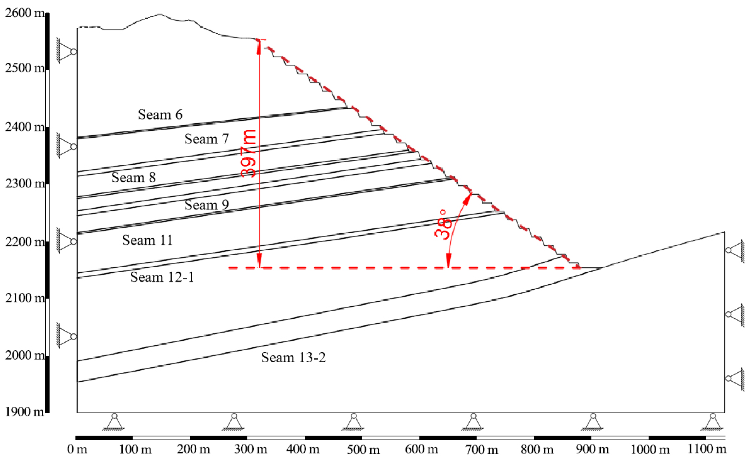
3.1. Engineering Situations

The proposed UPL optimization model was applied in a case study of a large open-pit coal mine in the semi-arid area of China. The surface topography of the mining area is shown in Figure 3a. Sections I–I and II–II, which represented the direction along the orebody trend and vertical to the orebody, respectively, are shown in Figure 3b. The mining region contains 10 coal seams, with seam 13-2 being the primary one. The coal reserves within this area amount to two billion tons. The dip angle of the orebody generally ranged from 13° to 25°, steeper angles of about 20° to 25° are observed deeper, while shallower sections range between 13° and 20°. The dip angle remains consistent in the strike direction, and the ore body tends to lean southward.

3.2. Natural Environmental Conditions

The Heishan open-pit coal mine is situated in the central region of Tianshan Mountain, characterized by a terrain that ascends in the north and west and descends in the south and east, ranging from an elevation of 2365 m to 3023 m. Vegetation transitions from grassland meadows to deserts from west to east, predominantly comprising grassland types. The floristic composition within the mine area is relatively simple, dominated by grasses such as sheep fescue, early harvest grassland, fine-leaved early harvest grass, needle fescue, and mixed grasslands, constituting excellent pastureland. In the eastern section of the mining area, the predominant vegetation is desert-type, characterized by sparse and homogenous distributions. The central area features a transitional vegetation type from grassland to desert, known as desert grassland. The predominant soil types in the mining area are chestnut calcium soil and brown calcium soil. Chestnut calcium soil, formed in semi-arid steppe regions under arid climatic conditions, exhibits weak leaching effects, significant calcification processes, and a pronounced carbonate precipitation layer. Vegetation on brown calcium soils, transitioning from steppe to desert, benefits from abundant light and heat resources, although water resources are limited.

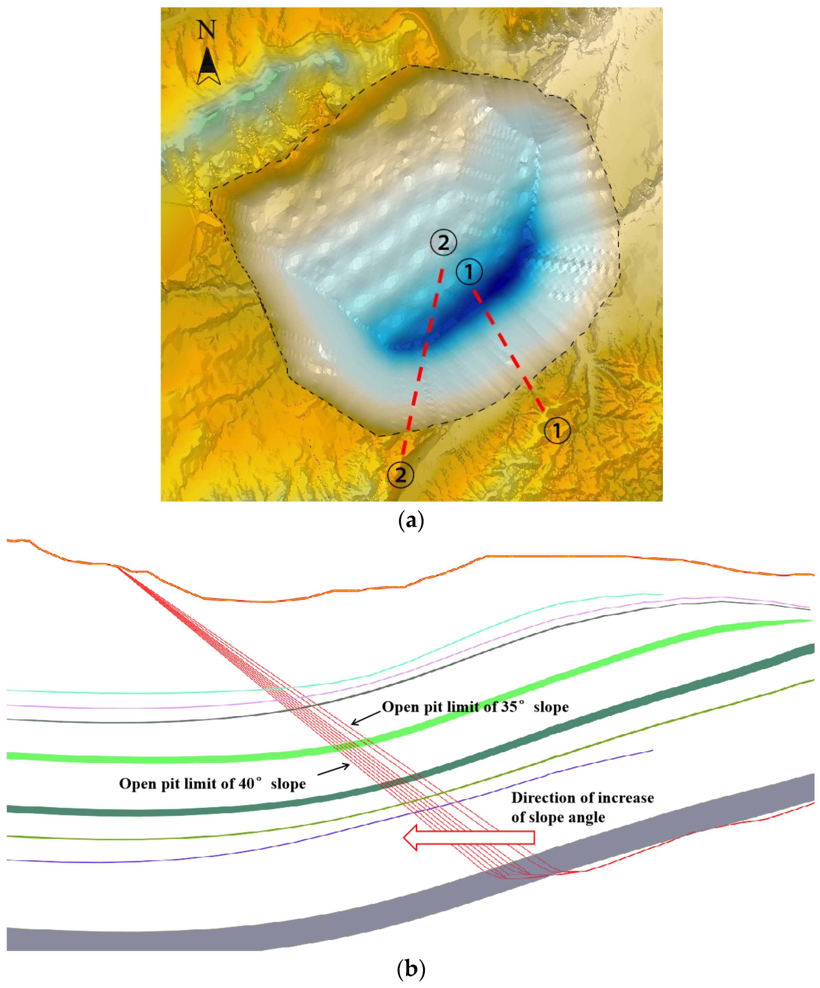
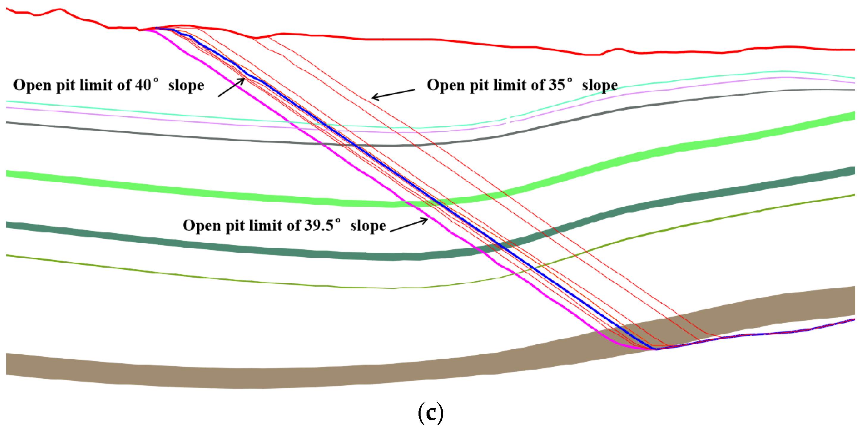
3.3. UPL Optimization Results for Heishan Open Pit Coal Mine

Coal preparation and washing costs were excluded from the UPL optimization due to the absence of beneficiation plants in the Heishan open-pit coal mine. The basic economic parameters used for UPL optimization are shown in

Table 3. Economic model parameters of Heishan open-pit coal mine.

Coal Price/(USD/t)	Coal Loss Thickness/m	Recovery Rate/%	Mining Cost of Rough Coal/(USD/t)	Cost of Rock Stripping/(USD/m3)	Stripping Cost of Quaternary Layer/(USD/m3)
26	0.2	96.5	1.62	2.18	1.16

. The slope angles of the Heishan open-pit coal mine in different azimuth ranges, as designed in the project drawings, are shown in

Table 4. Designed slope angles of UPL in different directions.

Azimuth Range of Slope	Slope Angle
0°~45°	17°
45°~135°	35°
135°~225°	35°
225°~315°	35°
315°~360°	17°

. These angles provided the foundational slope angles for UPL optimization. Based on the orebody occurrence condition, the mining of the northern wall was stripped along the orebody trend, thus primarily targeting the southern wall, with azimuth angles ranging from 225° to 315°.

Table 5. Designed slope angles and the UPL optimization results.

Scheme Number	Slope Angle /°	Quantity of Coal Mining /104 * t	Stripping Rock Volume /104 * t	Profit /MUSD	Stripping Ratio /(t·t−1)	Mining Depth /m
1	35.0	13,727.02	157,759.28	2001.66	10.11	397
2	36.0	13,889.91	160,852.05	2014.69	10.19	397
3	37.0	14,081.63	165,319.26	2022.76	10.33	402
4	37.5	14,148.18	166,592.23	2028.00	10.36	402
5	38.0	14,172.55	166,710.53	2032.97	10.35	402
6	38.5	14,163.53	165,977.78	2037.18	10.31	402
7	39.0	14,209.58	166,921.73	2040.26	10.34	407
8	39.5	14,302.44	169,232.73	2042.87	10.41	407
9	40.0	14,260.25	167,306.25	2049.38	10.32	407

shows the designed slope angles and the UPL optimization results based on the floating cone method under different slope angles.

As shown in Table 5, the quantities of coal mining and rock stripping generally increased with a steepening slope angle. However, there are exceptions, such as schemes, where coal mining volumes increase yet rock stripping decreases (slope angle = 39.5°), or both the quantities of coal mining and rock stripping decreased with steepening slope angle (slope angle = 38.5°, 40°). The total profit of UPLs consistently rose regardless of the variations in the quantities of ore and rock. This was because the profit from additional ore exceeded the cost of rock stripping when the quantities of coal mining and rock stripping increased with the steepening slope angle. Conversely, the profit loss from reduced ore mining was lesser than the savings from decreased rock stripping when both the quantities of coal mining and rock stripping decreased with the steepening slope angle. Therefore, steepening the slope angle would bring greater profit to mining. As a result, the steepening slope angle enhanced the total economic profit. For every 1° steepening of the slope angle of the open-pit coal mine, the total economic profit improved by an average of USD 9.54 M. The variations in slope angle significantly affected the total economic profit of the mine.

Figure 4a shows the 3D map of the UPL optimization results. Figure 4b,c show the sectional drawing of ①-① and ②-② in Figure 4a to compare the impact of slope angle modifications on UPL optimization results. As a result of the UPL optimization in Figure 4, the steepening strategy of the slope angle based on the float cone method could be summarized under the following conditions:

(1) The displacement outward from the pit bottom exceeded that from the pithead (e.g., transitions from 35° to 36° and from 36° to 37°);

(2) The outward displacement of the pit bottom was less than the inward contraction of the pithead (e.g., transitions from 38° to 38.5°);

(3) The pithead was fixed, and the pit bottom displaced outward (e.g., transitions from 37.5° to 38° and from 38.5° to 39°);

(4) The pit bottom stayed fixed, and the pithead contracted (e.g., transitions from 37° to 37.5° and transitions from 39° to 39.5°);

(5) The inward displacement of the pit bottom was less than the outward displacement of the pithead (e.g., transitions from 39.5° to 40°).

Different steepening schemes of the slope angle led to variations in the direction of slope expansion or contraction based on the floating cone optimization method. These findings suggested that even with a consistent steepening scheme of the slope angle, the result obtained from traditional designs might not always yield the highest economic value. Additionally, when adjusting the slope angle towards a specific direction, the primary alteration in the ultimate pit shape manifested in that direction and its adjacent areas, as illustrated by the end position. Intriguingly, changes could still occur in the mining location in other directions even if their slope angles remained consistent. This was because the floating cone method re-optimized the entire mining area, marking a significant departure from the conventional open-pit mine slope steepening approach.

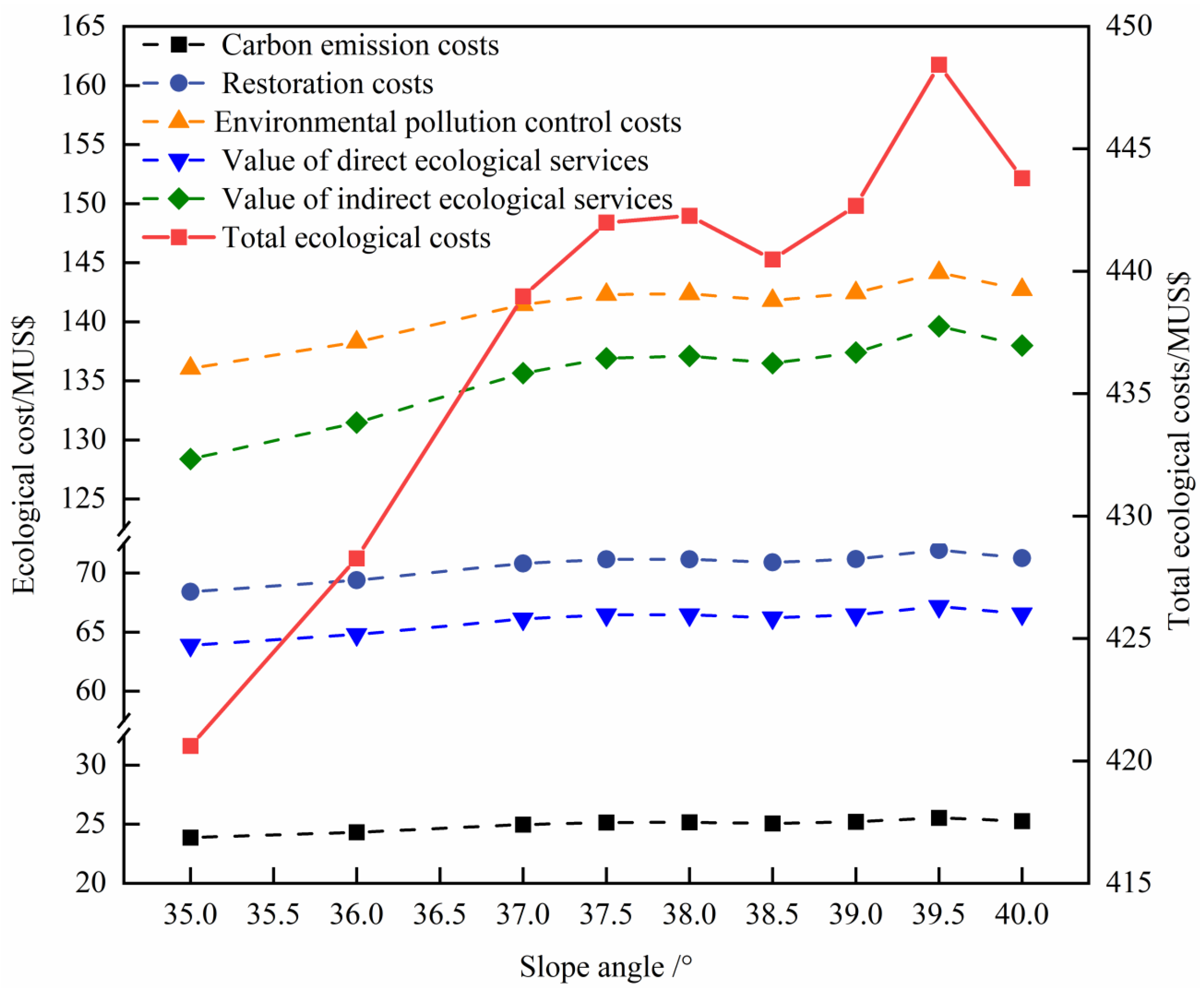
3.4. Ecological Cost of Heishan Open-Pit Coal Mine

The primary environmental consequences of mining activities in the Heishan open-pit coal mine contained the devastation of vegetation, air pollution, water contamination, and soil degradation. These impacts correlated predominantly with the land occupation of mining and the quantities and types of pollution emissions. The mine area with varying slope angles was determined by the UPL results. The area of the waste dump was calculated by Formula (1). Considering a similar production scale in different UPL schemes, the area allocated for handling official business, transportation, and the industrial site was taken as 20 hm². The area of land occupancy and damage in UPLs with different slope angles is shown in

Table 6. Designed slope angles and the UPL optimization results.

Scheme Number	Slope Angle/°	Mining Area/hm2	Dump Area/hm2	Other Area of Land Occupancy/hm2	Total Area of Land Destruction/hm2
1	35	510.75	615.26	20.00	1146.01
2	36	514.98	627.32	20.00	1162.30
3	37	521.10	644.75	20.00	1185.85
4	37.5	522.36	649.71	20.00	1192.07
5	38	521.91	650.17	20.00	1192.08
6	38.5	520.20	647.31	20.00	1187.51
7	39	521.10	650.99	20.00	1192.09
8	39.5	524.97	660.01	20.00	1204.98
9	40	521.19	652.49	20.00	1193.68

.

The ecological disruptions resulting from resource extraction share similarities across regions. However, regional variations existed in ecosystem functions and resilience to these disruptions. Additionally, the production scale and method of mining induced distinct ecological impacts. The calculation parameters of ecological cost are shown in

Table 7. Calculation parameters of ecological cost of Heishan open-pit coal mine.

Parameters	Quantitative Value	Parameters	Quantitative Value	Parameters	Quantitative Value	Parameters	Quantitative Value
cz/(USD/hm2)	55,752	ρ/(t/m3)	1.35	kNi/%	0.25	ca1/(USD/t)	188.6
K/%	35	r1/%	46	kPi/%	1.907	ca2/(USD/t)	2326.4
R/%	15	r2/%	15	cgi/(USD/hm2/a)	157	ca3/(USD/t)	80.88
J/(mm/a)	528.7	r3/%	50	Sbi/(USD/hm2/a)	735	qa1/(t/a)	49.5
$C_{H_{2}O}$/(USD/m3)	1	r4/%	50	$q_{ws}$/(m3/d)	4342	qa2/(t/a)	23.64
L/(USD/m3)	0.31	Qi/(t/hm2/a)	0.8277	cw1/(USD/m3)	0.8	qa3/(t/a)	6.88
Ρ1/(USD/m3)	1.4	$C_{O_2}$/(USD/t)	149.25	Cw2/(USD/m3)	0.83	V/(m3/m2)	0.002
Ρ2/(USD/m3)	0.85	h/m	0.5	α	2.625	T1/(USD/a)	19485
P31/(USD/t)	328.36	DSOC/(g/kg)	2.5	x	3	T2/(USD/a)	19485
P32/(USD/t)	119.4	DSIC/(g/kg)	7.5	ewt/(m3/t)	0.0008	ec/(kg/kWh)	0.404
P33/(USD/t)	405	$C_{{SO}_2}$/(USD/t)	188.06	λ	0.12	ηc/(t/t)	0.745
P34/(USD/t)	51	$C_{{CO}_2}$/(USD/t)	13.6	cst/USD/hm2	82610	vc/(kcal/kg)	7000
Mi/(t/hm2/a)	60.8	CD/(USD/t)	44.78	esw1/(kg/t)	4.676	ηh1/(t/t)	0.869
E1/%	0.0069	$Y_{{iSO}_2}$/(t/hm2/a)	0.0089	esw2/(kg/t)	0.00001	ηh2/(t/t)	0.854
E2/%	0.094	$Y_{iD}$/(t/hm2/a)	0.05	esw3/(kg/t)	0.0038	$e_e$/(kWh/t)	0.1
E3/%	2.28	pN/(USD/t)	328.36	esw4/(kg/t)	0.0009	$r_e$	0.8
E4/%	0.069	pP/(USD/t)	119.4	esw5/(kg/t)	0.0275	$e_{h2}$/(kg/t)	0.0031
qi/(t/hm2/a)	2.875	cr/(USD/hm2)	59701	$e_{h1}$/(kg/t)	0.29	$\mathrm{csw}4/(\mathrm{USD}/\mathrm{t})$	3.63
csw1/(USD/t)	0.73	csw2/(USD/t)	145	$\mathrm{csw}3/(\mathrm{USD}/\mathrm{t})$	3.63	$\mathrm{S}\mathrm{w}$	1.5
$e_{wt}$/(m3/d)	0.0008	HW/m	200	$\mathsf{\gamma }\mathrm{w}$	1.3	${\epsilon }_{st}$/%	10
$n_d$/d	330	$x_w$(n/d)	2	${\mathrm{V}}_{\mathrm{a}}$/(m3/m2)	0.002
ea1/(kg/t)	0.0003	ea2/(kg/t)	0.0001	ea3/(kg/t)	0.00004

Where E₁, E₂, E₃, and E₄ are the E_j in Formula (4); P₃₁, P₃₂, P₃₃, P₃₄ are the P_3j in Formula (4); e_sw1, e_sw2, e_sw3, e_sw4 are the e_swi in Formula (16); c_sw1, c_sw2, c_sw3, c_sw4 are the c_swi in Formula (16); c_a1, c_a2, c_a3 are the c_ai in Formula (17); η_h1, η_h2 are the η_hi in Formula (19); e_h1, e_h2 are the e_hi in Formula (19).

. These parameters were sourced from actual production data of the mine, market research, relevant national statistical yearbooks, and literature. The degradation value of grasslands from livestock manure was omitted since the mine site neither serves as a grazing area nor hosted a significant livestock population. Moreover, the amount of grassland (F) was taken as 1 because the mining site exclusively comprised one grassland type, the alpine desert grassland. The watering area of every time per day ($A_{nd}(\Phi )$) was calculated based on the annual average watering area for every time per day, 47 hm². According to the mine reclamation plan, the reclamation of damaged land will be completed in one year after the end of mining.

The mine is designed with an annual ore production capacity ($q_o(\Phi )$) of 10 million tons. The total ore quantity ($Q_o(\Phi )$) from the UPLs with different slope angles can be used to calculate the average annual stripping quantity, thereby obtaining the annual carbon emissions and other associated metrics of the open-pit mine. It is assumed that land acquisition and site preparation were finalized in the early phase of mining. Hence, the area of land occupancy and destruction after the first year of mining was calculated by $A_m(\Phi )+A_w(\Phi )+A_o$. Furthermore, it is presumed that the ecosystem of the mining area was recuperated three years post-mining ($n_t$). Based on these parameter configurations and the UPL optimization results under different slope angles, the ecological cost was calculated by Formula (23).

Figure 5 illustrates the ecological costs of the mine for each UPL scheme. In the traditional steepening approach of the open-pit mine slope, where the pit bottom was fixed and the pithead was contracted, the area of the mining field, the stripping volume of rock, and the occupied area of the mining decreased, thereby substantially diminishing the ecological impacts. However, the UPL scheme should be designed based on the ore body occurrence condition. With the steepening slope angle, the ecological cost and ore-rock volume increase, suggesting that the ecological cost is heavily influenced by the scale of mining. An anomaly occurs when the angle increases from 37.5° to 38°, and the ore rock volume surges by 1,426,700 tons. However, with the UPL slope steepened by fixing the pithead and the widening pit bottom, the UPL area decreased by 0.45 hm², leaving the ecological cost nearly the same. This disparity accentuates the primary distinction between the traditional steepening approach and the floating cone method. The former employs a steepening strategy in a set direction, while the latter evaluates the overarching impact of directional angle adjustments on the entire mining scope.

Figure 5 reveals the proportion of ecological costs to the cumulative ecological cost in arid or semi-arid lands. Specifically, the proportion of exogenous ecological value loss was 30.52%, the direct economic value loss was 15.19%, ecological costs from energy consumption were 5.67%, reclamation cost was 16.27%, and environmental pollution treatment costs were 32.35%. Within the UPL, considering the ratio of ecological costs to profits, the coal mining in semi-arid weak ecological land resulted in ecological costs that surpass 20% of the average pure economic gains from the mine. The combined contribution of energy consumption costs and exogenous ecological costs, which were not to be borne by enterprises, constituted over 35% of the total ecological cost. If these ecological value losses were integrated into the financial metrics of mining, the profit margins would face significant limitations.

3.5. Safety Cost of Heishan Open-Pit Coal Mine

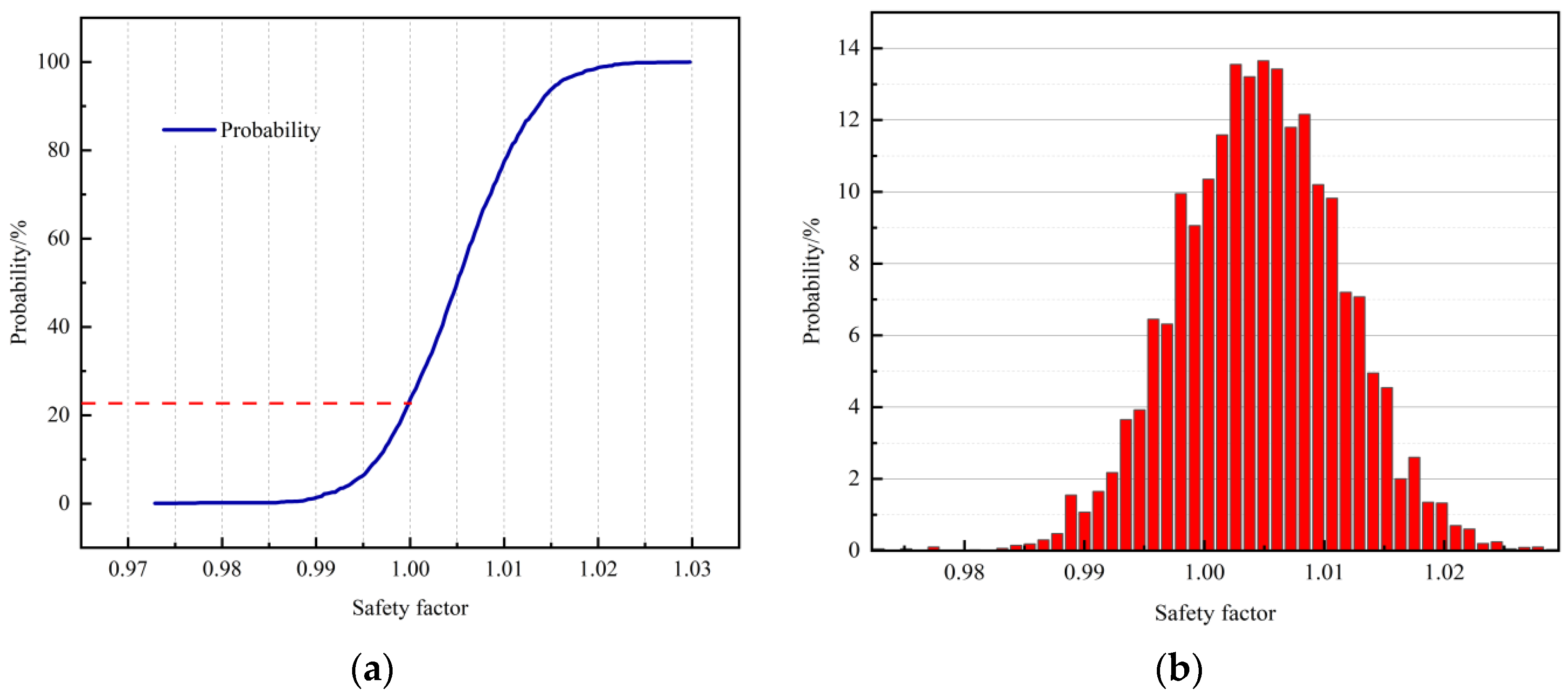
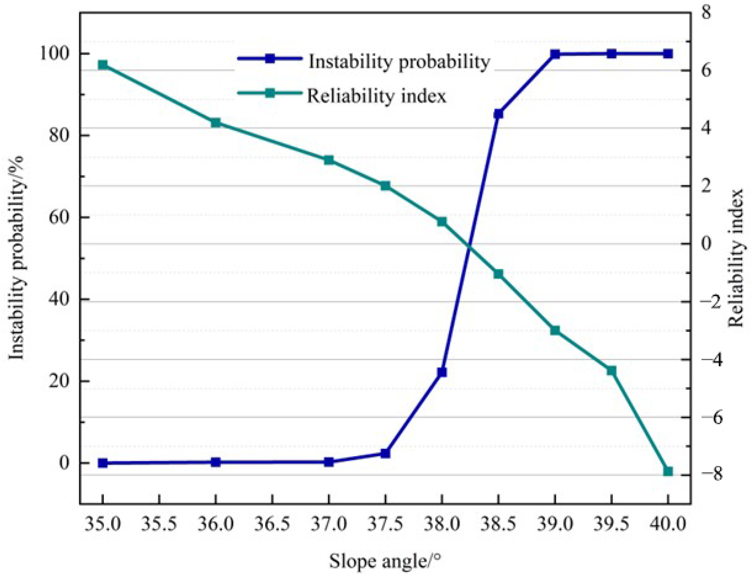
3.5.1. Stability Analysis of Open-Pit Coal Mine Slope

There was a contradiction in keeping the balance of slope stability and mining costs. While theoretically, slopes with a slope angle of 90° would be the most cost-effective for open pit mines, it was limited by the slope instability. To determine a reasonable slope geometry shape, the stability of slopes and the ecological impacts should be evaluated. The stability of slopes was influenced by various factors. In this study, only the main parameters, cohesion and the internal friction angle, were considered in the analysis of slope stability.

To analyze the instability probability of the south slope under various steepening schemes, we use the final realm derived from the 38° gang slope angle steepening scheme for the south gang as a reference. The profile is acquired at position ①-①, as depicted in Figure 3, and is further illustrated in Figure 6. The rock mass in the south area predominantly consists of mudstone and sandstone. To investigate the properties of these rocks, various samples were subjected to uniaxial compressive tests, Brazilian splitting tests, and triaxial tests to determine their strength parameters. It is hypothesized that the uniaxial compressive strength, tensile strength, cohesive force, angle of internal friction, and other mechanical parameters follow a normal distribution. Previous research has predominantly applied the geotechnical parameter random field to three-dimensional conditions [50,51], though some studies have also explored the random distribution characteristics under two-dimensional conditions [52,53]. Owing to the larger scale and more complex lithology of open-pit mine slopes, this study focuses solely on the random distribution of geotechnical parameters under two-dimensional conditions, aiming to simplify the calculation of slope reliability.

Table 8. Physical and mechanical properties of rock in typical layers.

		Density/g·cm−3	Uniaxial Compressive Strength/MPa	Tensile Strength/MPa	Cohesion/MPa	Internal Friction Angle/°
Mudstone	Statistical number	21	15	15	10	10
	Mean value	2.61	7.76	0.46	0.41	30.08
	Variance	0.1	6.54	0.33	0.34	1.60
	Coefficient of variation	0.04	0.84	0.71	0.81	0.05
Sandstone	Statistical number	84	26	27	80	80
	Mean value	2.4	25.95	1.49	3.35	38.61
	Variance	0.1	10.68	0.84	1.39	11.47
	Coefficient of variation	0.04	0.41	0.56	0.41	0.29

shows the cohesion and internal friction angle of typical layers in the Heishan open-pit coal mine. Due to the minimal variance mechanical properties of coal, the weight of coal was taken as 12.9 kN/m³, with a cohesion of 1.32 MPa and an internal friction angle of 34°.

The Monte Carlo method was used to compute the landslide risk probability. The analysis primarily focuses on randomly sampling factors that influence slope stability (i.e., internal friction angle and cohesion) with a sample size of 15,000 experiments. Subsequently, stability analyses were performed using the Geostudio (Slope/W) module in the Geostudio geotechnical software. The impact of pore water pressure on reliability was excluded from the analysis. The safety coefficient of the slope model for various slope angles was calculated by using the simplified Bishop’s method. The Mohr–Coulomb model was adopted for the geotechnical modeling. The risk assessment revealed the critical sliding surface of the UPL slope for a slope angle of 38°, as illustrated in Figure 7.

Figure 8a,b display the probability density function of the safety coefficient and the probability distribution function for a safety coefficient lower than 1.0, both derived from the Monte Carlo simulation (with a slope angle of 38°). The reliability index for the slope was determined to be 0.77, with an instability probability of 22.15%. Similarly, the instability probability and reliability index of the slope with different slope angles could be deduced. The results of these calculations are presented in Figure 9.

Figure 9 revealed that as the slope angle steepened, the slope reliability index diminished, leading to a concomitant rise in the instability probability. At a slope angle of 35°, the slope reliability index was 6.2, surpassing the target reliability index of 3.2. However, when the slope angle was steepened to 37°, the reliability index fell to 2.79, below the target reliability threshold, presenting a 0.2% probability of instability.

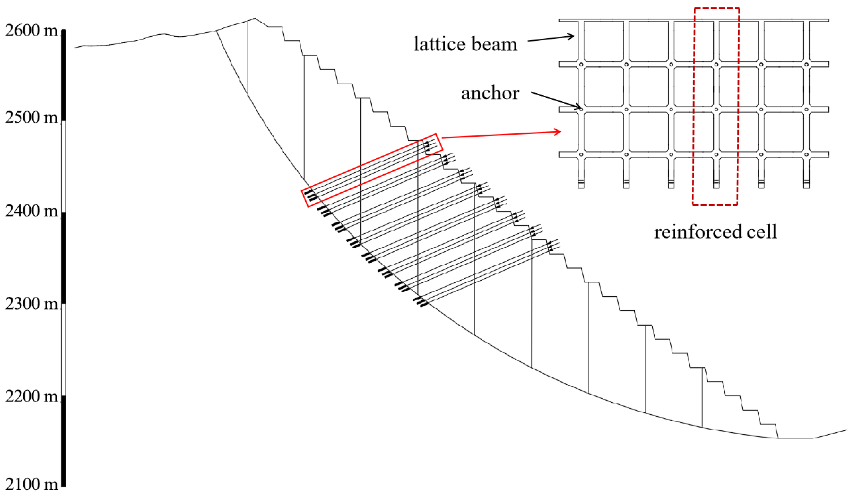
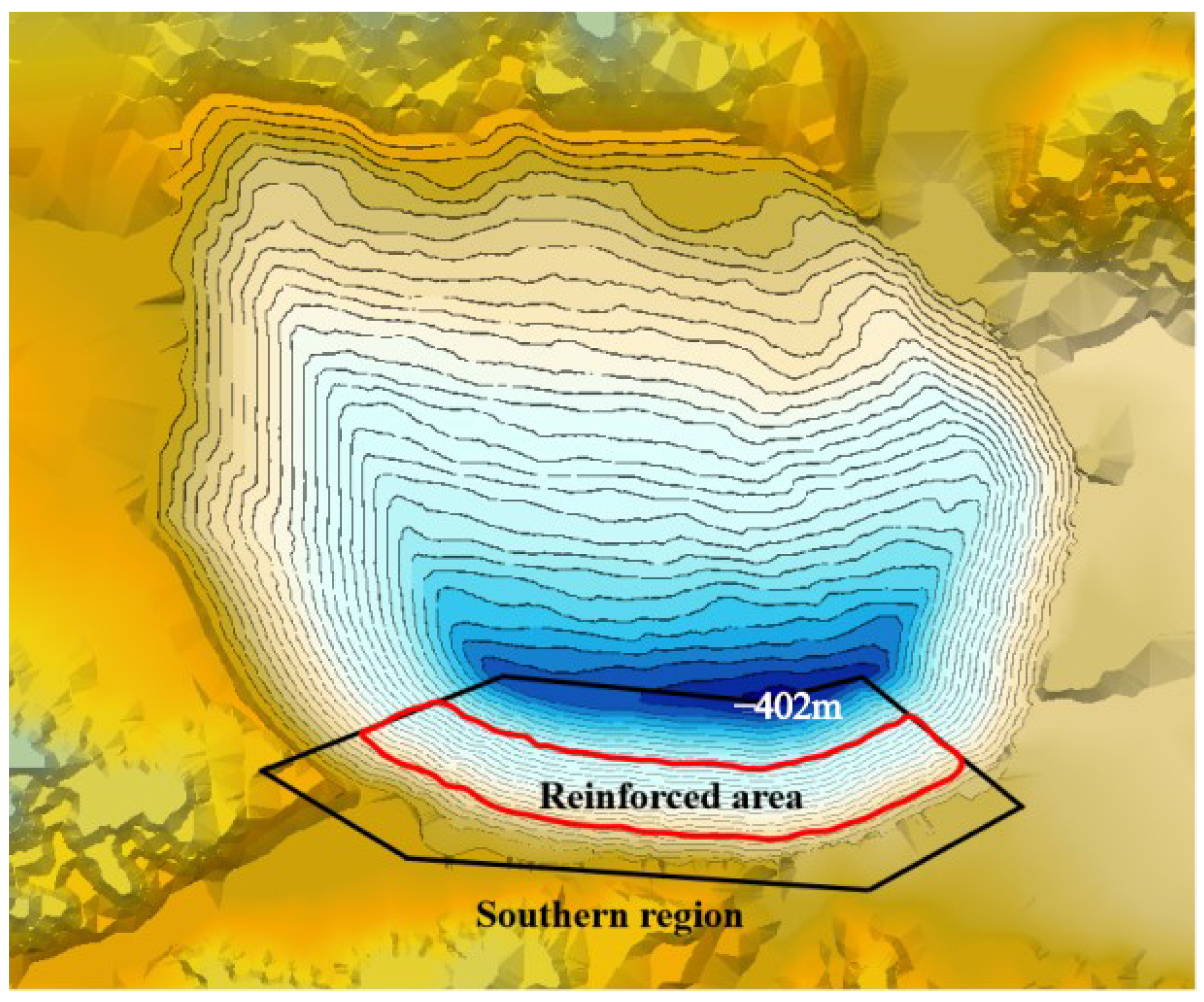
3.5.2. Reinforcement Plan Selection and Safety Cost Calculation of Heishan Open-Pit Coal Mine

Given that the anchor lattice beam structure was more apt for supporting rocky slopes in open-pit mines, this structure was employed to reinforce potential landslide regions within the Heishan open-pit coal mine. Figure 10 presents a schematic representation of the anchor lattice beam reinforcement design. The design process primarily contained two main aspects: the configuration of the anchors and the formulation of the lattice beam. The design parameters for the anchorage angle were set at 20° with a vertical spacing of 4 m. The orifice diameter was 150 mm. M30 cement mortar was used as the grouting material. The section dimensions of the lattice beam were 400 mm × 400 mm, with its primary reinforcement at the top and bottom being 2Φ22 and the hoop reinforcement being Φ8@150. The concrete used for pouring was selected as the C30 concrete. Additional specifications are detailed in

Table 9. Reinforcement parameters of anchor lattice beam in different UPL schemes.

Slope Angle/°	Dimensions of Steel Strands	Anchoring Length/m	Row Number of Anchor Cable
37	4 × 7Φ5	3	21
37.5	4 × 7Φ5	3	21
38	5 × 7Φ5	3	27
38.5	5 × 7Φ5	3	39
39	5 × 7Φ5	3	51
39.5	5 × 7Φ5	4	60
40	6 × 7Φ5	4	69
37	4 × 7Φ5	3	21

.

The reinforcement cost calculation model was introduced as an example for a slope angle of 38°. The initial step involved determining the reinforcement area and strategy based on slope stability analysis and the reinforcement design scheme. As shown in Figure 10, the black region represents the south-steepened slope, while the red shows the potential landslide reinforcement region. Subsequently, the reinforcement phases were segmented into multiple reinforcement units. For instance, the red zone in Figure 11 symbolizes a single reinforcement unit. The total number of such units for every reinforcement phase was dictated by the top and bottom lines of the steps within the reinforcement region. To further detail the method, one should measure the length of the free end across three rows of anchors for every reinforcement phase. The required strand length for each anchor hole was derived from the cumulative length of the tension section, free end, and anchorage section, multiplied by the strand count. The volume of the grouting material was determined by the length of the anchorage section being multiplied by the area of the anchor hole. The volume of the concrete used for pouring the lattice girder was deduced from the design schematic, with the respective volumes of the top girder, longitudinal girder, beams, and foundation being incorporated. The lengths of the reinforcement bars for the lattice girder, as well as the reinforcement length of the girder itself, were derived from the design scheme. Once the volume for each project segment has been evaluated, the cost of slope reinforcement for different slope angles can be calculated by using the bill of quantities. The i-th type of sub-projects (Pi) was determined based on the engineering quotas released by the local government. The reinforcement costs of the slope using the anchor lattice beam are detailed in

Table 10. Reinforcement cost of anchor lattice beam in different UPL schemes.

Slope angle/°	37	37.5	38	38.5	39	39.5	40
Reinforcement cost/MUSD	10.31	10.82	14.42	19.08	25.67	30.04	41.54
Instability probability/%	0.25	2.35	22.5	85.35	99.85	100	100
Potential reinforcement cost/MUSD	0	0.25	3.24	16.28	25.67	30.04	41.54

. It is observed that as the slope angle increased, the instability probability of the slope also increased, leading to a significant rise in the required support works and associated costs. The larger investments in support and higher maintenance costs were necessitated to ensure the stability of the slope. This presented a contradiction: while a steeper slope angle may yield better pure economic benefits, it simultaneously demands greater safety costs. Thus, a slope angle that can balance both economic and safety considerations for the mine must be determined.

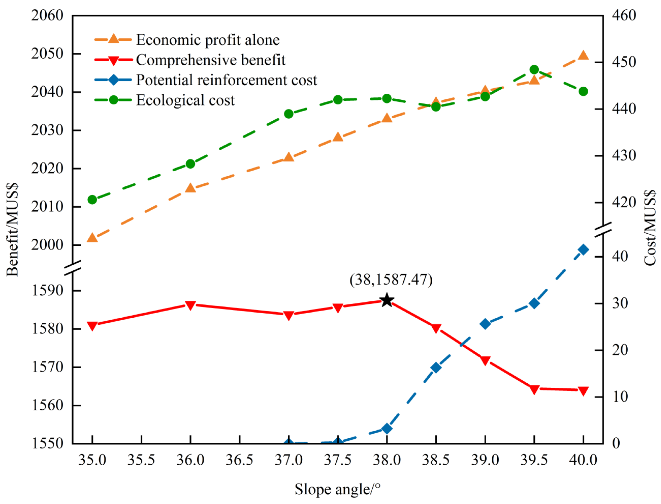
3.6. Comprehensive Benefit Analysis of Different UPLs

Figure 12 shows the pure economic profit, ecological cost, and safety cost (reinforcement cost) associated with each UPL under varying slope angle schemes. When solely considering the economic benefits of mining, a larger slope angle was preferred. However, from an ecological perspective, a smaller slope angle was generally more advantageous. The ecological cost was influenced by factors such as ore rock volume and area of land degradation, observations which contrasted with the traditional steepening method. From a safety standpoint, gentler slope angles were safer, necessitating lower costs for slope reinforcement. For slope angles ranging from 35° to 38°, the economic benefits derived from increasing the slope angle surpass the associated rise in ecological and reinforcement costs. On the other hand, for slope angles from 38° to 40°, augmented costs related to ecology and slope maintenance outweigh the economic advantages, with the reinforcement costs for the slope escalating notably as the angle steepens. The comprehensive economic benefits, which integrated consideration of ecological cost, slope reinforcement cost, and stripping benefits, peaked at USD 1587.47 M at a slope angle of 38°.

Figure 13 illustrates the UPL optimization results based on three considerations: solely for maximum economic benefits of mining (with a slope angle of 40°), accounting for ecological impact and slope stability (with a slope angle of 35°), and integrated consideration of economic, ecological environment, and safety factors (with a slope angle of 38°). Compared with the original design of UPL (with a slope angle of 35°), the comprehensive UPL optimization (with a slope angle of 38°) displayed the following variations:

(1) The rock stripping quantity increased by 3580.5 m³.

(2) The direct land degradation area expanded by 46.07 hm².

(3) The ecological cost has surged by USD 21.65 M.

(4) The instability probability of the slope has grown by 22.5%, leading to a potential consolidation cost increase of USD 3.24 M.

(5) The pure economic benefit has increased by USD 31.31 M.

(6) The combined profit integrated consideration of ecological environment, slope safety, and economic benefits increased by USD 6.42 M.

(7) The resource recovery of coal increased by 4,455,300 tons.

The estimation of slope instability probability can be enhanced by utilizing a three-dimensional model, thereby achieving higher precision. Nevertheless, given the vast scale and complex geological features of open-pit mines, constructing such a three-dimensional model presents significant challenges. Consequently, in this study, we use a widely adopted two-dimensional simplified model for open-pit slope analysis to estimate the likelihood of slope instability [52,53,54,55]. In future research, we aim to develop a precise three-dimensional geological model specifically tailored to assess the potential for slope failure.

Based on the results of this study, the concept of sustainable development in open pit mines can be expanded to encompass the entire mining cycle, addressing four key aspects: economy, efficiency, environment, and safety. This UPL optimization method offers a comprehensive interpretation of sustainability and integrates the principles of greenness, efficiency, and safety into mine design. Additionally, the quantitative evaluation of environmental impacts detailed in this study could be applied to the coal industry or related sectors, such as metallurgy [56].

4. Conclusions

This study focuses on the UPL, which profoundly impacts the economic benefit, ecological impact, and the geometric of mine slope optimization method by integrating considerations of ecological environment, slope safety, and economic benefit. The proposed UPL optimization method, which considers multiple sustainability factors, paves the way for environmentally friendly, low-carbon, safe, and efficient mining in open-pit coal mines. The primary findings include:

(1) Compared with the conventional design approach, the optimization based on the floating cone method prioritizes an integrative design encompassing the entire mining region, which reveals unpredictable variations in the extension direction of UPL slope and the ore volume of mining. In the case study of an open-pit coal mine, there was an average economic profit rise of 9.54M USD with every 1° increase in slope angle.

(2) As the slope angle steepened, the ecological cost fluctuation pattern aligns closely with the ore and rock quantities in UPLs. This indicates that the ecological cost is closely impacted on the mining scale.

(3) In arid or semi-arid weak ecological land, the environmental pollution control costs during mining and exogenous ecological value losses are paramount contributors to the overall ecological cost. In terms of the ratio between ecological costs and profits within the UPL, the coal mining in Xinjiang’s semi-arid weak ecological land imposes ecological costs exceeding 20% of the mines’ average pure economic gains. The proportion of energy consumption cost and exogenous ecological cost (which is not to be borne by enterprises) to the total ecological cost reaches more than 35%.

(4) For slacken slope angles, the increment of economic benefits caused by steepening the slope angle is higher than the increased ecological and reinforcement costs. Conversely, for steeper slope angles, the cost increments in ecology and slope maintenance surpass the economic gains, especially in the reinforcement costs of the slope, which soar dramatically with the slope angle. In the case study, the comprehensive benefits of mining peak at USD 1587.47 M at a slope angle of 38°. Meanwhile, the resource recovery rate increased by 3.25%.

References

1. Auty, R.; Warhurst, A. Sustainable development in mineral exporting economies. Resour. Policy 1993, 19, 14–29. [Google Scholar] [CrossRef]
2. Mikesell, R.F. Sustainable development and mineral resources. Resour. Policy 1994, 20, 83–86. [Google Scholar] [CrossRef]
3. Hilson, G.; Murck, B. Sustainable development in the mining industry: Clarifying the corporate perspective. Resour. Policy 2000, 26, 227–238. [Google Scholar] [CrossRef]
4. Horowitz, L. Section 2: Mining and sustainable development. J. Clean. Prod. 2006, 14, 307–308. [Google Scholar] [CrossRef]
5. Hilson, G.; Basu, A.J. Devising indicators of sustainable development for the mining and minerals industry: An analysis of critical background issues. Int. J. Sustain. Dev. World Ecol. 2003, 10, 319–331. [Google Scholar]
6. Azapagic, A. Developing a framework for sustainable development indicators for the mining and minerals industry. J. Clean. Prod. 2004, 12, 639–662. [Google Scholar] [CrossRef]
7. Adibi, N.; Ataee-pour, M.; Rahmanpour, M. Integration of sustainable development concepts in open pit mine design. J. Clean. Prod. 2015, 108, 1037–1049. [Google Scholar] [CrossRef]
8. Amirshenava, S.; Osanloo, M. A hybrid semi-quantitative approach for impact assessment of mining activities on sustainable development indexes. J. Clean. Prod. 2019, 218, 823–834. [Google Scholar] [CrossRef]
9. Ebrahimi, M.; Rahmani, D. A five-dimensional approach to sustainability for prioritizing energy production systems using a revised GRA method: A case study. Renew. Energy 2019, 135, 345–354. [Google Scholar] [CrossRef]
10. Que, S.; Awuah-Offei, K.; Demirel, A.; Wang, L.; Demirel, N.; Chen, Y. Comparative study of factors affecting public acceptance of mining projects: Evidence from USA, China and Turkey. J. Clean. Prod. 2019, 237, 117634. [Google Scholar] [CrossRef]
11. Hosseinpour, M.; Osanloo, M.; Azimi, Y. Evaluation of positive and negative impacts of mining on sustainable development by a semi-quantitative method. J. Clean. Prod. 2022, 366, 132955. [Google Scholar] [CrossRef]
12. Dehghani, H.; Bascompta, M.; Khajevandi, A.A.; Farnia, K.A. A Mimic Model Approach for Impact Assessment of Mining Activities on Sustainable Development Indicators. Sustainability 2023, 15, 2688. [Google Scholar] [CrossRef]
13. Laurence, D. Establishing a sustainable mining operation: An overview. J. Clean. Prod. 2011, 19, 278–284. [Google Scholar] [CrossRef]
14. Asr, E.T.; Kakaie, R.; Ataei, M.; Tavakoli Mohammadi, M.R. A review of studies on sustainable development in mining life cycle. J. Clean. Prod. 2019, 229, 213–231. [Google Scholar]
15. Xu, X.C.; Gu, X.W.; Wang, Q.; Gao, X.; Liu, J.P.; Wang, Z.K.; Wang, X.H. Production scheduling optimization considering ecological costs for open pit metal mines. J. Clean. Prod. 2018, 180, 210–221. [Google Scholar] [CrossRef]
16. Xu, X.C.; Gu, X.W.; Wang, Q.; Zhao, Y.Q.; Wang, Z.K. Open pit limit optimization considering economic profit, ecological costs and social benefits. Trans. Nonferrous Met. Soc. China 2021, 31, 3847–3861. [Google Scholar]
17. Xu, X.C.; Gu, X.W.; Wang, Q.; Zhao, Y.Q.; Zhu, Z.G.; Wang, F.D.; Zhang, Z.L. Ultimate pit optimization with environmental problem for open-pit coal mine. Process Saf. Environ. Prot. 2023, 173, 366–372. [Google Scholar]
18. Feng, H.; Zhou, J.; Chai, B.; Zhou, A.; Li, J.; Zhu, H.; Chen, H.; Su, D. Groundwater environmental risk assessment of abandoned coal mine in each phase of the mine life cycle: A case study of Hongshan coal mine, North China. Environ. Sci. Pollut. Res. 2020, 27, 42001–42021. [Google Scholar]
19. Qi, P.; Shang, Y. Evaluation of Environmental Quality for Abandoned Coal Mine Based on Environmental Vulnerability Index. Energy Eng. 2021, 118, 727–736. [Google Scholar]
20. Sun, Y.H.; Li, J.; Zhang, C.Y.; Li, F.Y.; Chen, W.; Ying, L. Environment monitoring of mining area with comprehensive mining ecological index (CMEI): A case study in Xilinhot of Inner Mongolia, China. Int. J. Sustain. Dev. World Ecol. 2023, 30, 814–825. [Google Scholar] [CrossRef]
21. Marshall, A. Principles of Economics; Macmillan & Co.: London, UK; New York, NY, USA, 1890. [Google Scholar]
22. Ugochukwu, U.C.; Chukwuone, N.; Jidere, C.; Ezeudu, B.; Ikpo, C.; Ozor, J. Heavy metal contamination of soil, sediment and water due to galena mining in Ebonyi State Nigeria: Economic costs of pollution based on exposure health risks. J. Environ. Manag. 2022, 321, 115864. [Google Scholar] [CrossRef]
23. Badakhshan, N.; Shahriar, K.; Afraei, S.; Bakhtavar, E. Determining the environmental costs of mining projects: A comprehensive quantitative assessment. Resour. Policy 2023, 82, 103561. [Google Scholar]
24. Badiozamani, M.M.; Askari-Nasab, H. Integration of reclamation and tailings management in oil sands surface mine planning. Environ. Model. Softw. 2014, 51, 45–58. [Google Scholar] [CrossRef]
25. Singh, V.K.; Singh, J.K.; Kumar, A. Geotechnical study for optimizing the slope design of a deep open-pit mine, India. Bull. Eng. Geol. Environ. 2005, 64, 301–306. [Google Scholar]
26. Islam, M.R.; Faruque, M.O. Optimization of slope angle and its seismic stability: A case study for the proposed open pit coalmine in Phulbari, NW Bangladesh. J. Mt. Sci. 2013, 10, 976–986. [Google Scholar]
27. Ren, S.L.; Tao, Z.G.; He, M.C.; Pang, S.H.; Li, M.N.; Xu, H.T. Stability analysis of open-pit gold mine slopes and optimization of mining scheme in Inner Mongolia, China. J. Mt. Sci. 2020, 17, 2997–3011. [Google Scholar]
28. Singh, V.K.; Singh, T.N. Geotechnical study of the optimum design of the Chandmari Coppermine, Rajasthan, India. Eng. Geol. 1999, 53, 47–55. [Google Scholar]
29. Cai, M.; Xie, M.; Li, C. GIS-based 3D limit equilibrium analysis for design optimization of a 600 m high slope in an open pit mine. J. Univ. Sci. Technol. Beijing 2007, 14, 1–5. [Google Scholar]
30. Shen, J.; Priest, S.D.; Karakus, M. Determination of Mohr–Coulomb Shear Strength Parameters from Generalized Hoek–Brown Criterion for Slope Stability Analysis. Rock Mech. Rock Eng. 2011, 45, 123–129. [Google Scholar]
31. Ozbay, A.; Cabalar, A.F. FEM and LEM stability analyses of the fatal landslides at Çöllolar open-cast lignite mine in Elbistan, Turkey. Landslides 2014, 12, 155–163. [Google Scholar] [CrossRef]
32. Dyson, A.P.; Tolooiyan, A. Prediction and classification for finite element slope stability analysis by random field comparison. Comput. Geotech. 2019, 109, 117–129. [Google Scholar] [CrossRef]
33. Ghadrdan, M.; Dyson, A.P.; Shaghaghi, T.; Tolooiyan, A. Slope stability analysis using deterministic and probabilistic approaches for poorly defined stratigraphies. Geomech. Geophys. Geo-Energy Geo-Resour. 2020, 7, 1–17. [Google Scholar] [CrossRef]
34. Kring, K.; Chatterjee, S. Uncertainty quantification of structural and geotechnical parameter by geostatistical simulations applied to a stability analysis case study with limited exploration data. Int. J. Rock Mech. Min. Sci. 2020, 125, 104157. [Google Scholar] [CrossRef]
35. Shang, L.; Nguyen, H.; Bui, X.N.; Vu, T.H.; Costache, R.; Hanh, L.T.M. Toward state-of-the-art techniques in predicting and controlling slope stability in open-pit mines based on limit equilibrium analysis, radial basis function neural network, and brainstorm optimization. Acta Geotech. 2021, 17, 1295–1314. [Google Scholar] [CrossRef]
36. Lu, Y.; Jin, C.; Wang, Q.; Han, T.; Li, G.; Zhong, X.; Chen, G. Combining InSAR and infrared thermography with numerical simulation to identify the unstable slope of open-pit: Qidashan case study, China. Landslides 2023, 20, 1961–1974. [Google Scholar]
37. Buelga Díaz, A.; Diego Álvarez, I.; Castañón Fernández, C.; Krzemień, A.; Iglesias Rodríguez, F.J. Calculating ultimate pit limits and determining pushbacks in open-pit mining projects. Resour. Policy 2021, 72, 102058. [Google Scholar] [CrossRef]
38. Jelvez, E.; Morales, N.; Ortiz, J.M. Stochastic Final Pit Limits: An Efficient Frontier Analysis under Geological Uncertainty in the Open-Pit Mining Industry. Mathematics 2021, 10, 100. [Google Scholar] [CrossRef]
39. Williams, J.; Singh, J.; Kumral, M.; Ramirez Ruiseco, J. Exploring Deep Learning for Dig-Limit Optimization in Open-Pit Mines. Nat. Resour. Res. 2021, 30, 2085–2101. [Google Scholar]
40. Deutsch, M.; Dağdelen, K.; Johnson, T. An Open-Source Program for Efficiently Computing Ultimate Pit Limits: MineFlow. Nat. Resour. Res. 2022, 31, 1175–1187. [Google Scholar]
41. Turan, G.; Onur, A.H. Optimization of open-pit mine design and production planning with an improved floating cone algorithm. Optim. Eng. 2022, 24, 1157–1181. [Google Scholar] [CrossRef]
42. Ares, G.; Castañón Fernández, C.; Álvarez, I.D. Ultimate Pit-Limit Optimization Algorithm Enhancement Using Structured Query Language. Minerals 2023, 13, 966. [Google Scholar] [CrossRef]
43. Stanek, W.; Czarnowska, L.; Pikoń, K.; Bogacka, M. Thermo-ecological cost of hard coal with inclusion of the whole life cycle chain. Energy 2015, 92, 341–348. [Google Scholar]
44. Fang, H.W.; Chen, Y.; Deng, X.W. A new slope optimization design based on limit curve method. J. Cent. South Univ. 2019, 26, 1856–1862. [Google Scholar]
45. Altuntov, F.K.; Erkayaoğlu, M. A New Approach to Optimize Ultimate Geometry of Open Pit Mines with Variable Overall Slope Angles. Nat. Resour. Res. 2021, 30, 4047–4062. [Google Scholar]
46. Wang, J.P.; Huang, D. RosenPoint: A Microsoft Excel-based program for the Rosenblueth point estimate method and an application in slope stability analysis. Comput. Geosci. 2012, 48, 239–243. [Google Scholar] [CrossRef]
47. Ahmadabadi, M.; Poisel, R. Assessment of the application of point estimate methods in the probabilistic stability analysis of slopes. Comput. Geotech. 2015, 69, 540–550. [Google Scholar]
48. Low, B.K. Context-Dependent Parameter Sensitivities in Rock Slope Stability. Rock Mech. Rock Eng. 2022, 55, 7445–7468. [Google Scholar] [CrossRef]
49. Wu, S.; Zhang, H.; Xiao, S.; Han, L. Study on time-varying target reliability of open-pit slope considering service life. J. Min. Saf. Eng. 2019, 36, 542–548. [Google Scholar]
50. Chen, X.J.; Fang, P.P.; Chen, Q.N.; Hu, J.; Yao, K.; Liu, Y. Influence of cutterhead opening ratio on soil arching effect and face stability during tunnelling through non-uniform soils. Undergr. Space 2024, 17, 45–59. [Google Scholar] [CrossRef]
51. Cheng, P.; Liu, Y.; Li, Y.P.; Yi, J.T. A large deformation finite element analysis of uplift behaviour for helical anchor in spatially variable clay. Comput. Geotech. 2023, 141, 104542. [Google Scholar] [CrossRef]
52. Zevgolis, I.E.; Deliveris, A.V.; Koukouzas, N.C. Probabilistic design optimization and simplified geotechnical risk analysis for large open pit excavations. Comput. Geotech. 2018, 103, 153–164. [Google Scholar] [CrossRef]
53. Peng, X.; Li, D.; Cao, Z.; Tang, X.; Zhou, C. Reliability-based design approach of rock slopes using Monte Carlo simulation. Chin. J. Rock Mech. Eng. 2016, 35, 3794–3804. [Google Scholar] [CrossRef]
54. Liu, F.Y.; Yang, T.H.; Zhou, J.R.; Deng, W.X.; Yu, Q.L.; Zhang, P.H.; Cheng, G.W. Spatial Variability and Time Decay of Rock Mass Mechanical Parameters: A Landslide Study in the Dagushan Open-Pit Mine. Rock Mech. Rock Eng. 2020, 53, 3031–3053. [Google Scholar] [CrossRef]
55. Zhang, H.J.; Wu, S.C.; Zhang, Z.X.; Huang, S.G. Reliability analysis of rock slopes considering the uncertainty of joint spatial distributions. Comput. Geotech. 2023, 161, 105566. [Google Scholar]
56. Yashalova, N.N.; Potravny, I.M. Possibilities of applying ESG-principles and methods of climate financing in the management practice of ferrous metallurgy enterprises. Chernye Met. 2023, 5, 76–81. [Google Scholar]
Figure 1. The 3D cone and conical shell template; (a) 3D cone; (b) cone shell template.
Sustainability 16 05393 g001
Figure 2. Framework of the UPL optimization model.
Sustainability 16 05393 g002
Figure 3. Geologic topographic map of Heishan open-pit coal mine. (a) Surface topographic map. (b) Geological section map.
Sustainability 16 05393 g003
Figure 4. Geologic-topographic map of Heishan open-pit coal mine: (a) 3D diagram of UPL scheme; (b) UPL schemes with different slope angles in section ①-①; (c) UPL schemes with different slope angles in section ②-②.
Sustainability 16 05393 g004aSustainability 16 05393 g004b
Figure 5. Ecological cost calculated from UPL schemes with different slope angles.
Sustainability 16 05393 g005
Figure 6. Slope reliability analysis model based on the Monte Carlo method (an example with slope angle of 38°).
Sustainability 16 05393 g006
Figure 7. The range of landslide mass (an example with a slope angle of 38°).
Sustainability 16 05393 g007
Figure 8. Probability density function of slope safety factor (an example with a slope angle of 38°). (a) Cumulative distribution curve of the probability density function. (b) Distribution histogram of probability density function.
Sustainability 16 05393 g008
Figure 9. Curves of slope reliability and instability probability in different slope angles.
Sustainability 16 05393 g009
Figure 10. Schematic diagram of anchor lattice beam reinforcement structure.
Sustainability 16 05393 g010
Figure 11. Schematic diagram of reinforcement area in South slope (an example with a slope angle of 38°).
Sustainability 16 05393 g011
Figure 12. Economic profit of UPL schemes with different slope angles.
Sustainability 16 05393 g012
Figure 13. Comparison of UPL schemes integrated considering single and multiple factors.
Sustainability 16 05393 g013