Abstract
The chain reaction of bridge abutment structure caused by frost heave of the embankment–bridge transition zone filler in cold regions has a great impact on the smoothness of railway lines, which will bring great challenges to the normal operation, safety, and maintenance of rail transit in cold regions under the action of long-term dynamic load. In this paper, the hydrothermal model and dynamic analysis model of the embankment–bridge transition zone are established, and the frost heave deformation rule and dynamic response characteristics of the embankment–bridge transition zone under frost heave conditions are studied. The results show that the effect of the bridge abutment structure on vertical frost heave is mainly concentrated in the range of the bridge abutment, and the vertical frost heave near the abutment is much smaller than other parts away from the abutment. The dynamic response and wheel–rail contact force of the embankment–bridge transition zone are significantly different under non-frost heave and frost heave conditions. Frost heave may cause a higher risk of derailment. This study provides a scientific reference for the design, construction, and safe operation and maintenance of embankment–bridge transition zones in cold regions, and has certain practical engineering significance.
1. Introduction
The embankment–bridge transition zone is an important part of railway lines. However, for the transition zone in cold regions, frost heave of filler will lead to a chain reaction of deformation and displacement of abutment structure, which has a great impact on the smoothness of railway lines and seriously affects the safety of railway operation under the joint action of a long-term dynamic load of trains. This brings great challenges to the maintenance of the embankment–bridge transition zone in cold regions. Therefore, it is of great significance to study the frost heave deformation and dynamic response characteristics of the embankment–bridge transition zone of railways under frost heave conditions in cold regions.
As for research on frost heave deformation of engineering in cold regions, Taber first carried out preliminary exploratory research on frost heave in 1929. From then until the end of the 20th century, Miller, Gilpin, and Sheng carried out further research on numerical simulation of frost heave. During this period, several main modeling methods for frost heave simulation were developed, including the hydrodynamic model, the rigid ice model, and the fractional condensation potential model [1,2,3,4,5,6]. In recent years, many relevant researchers have carried out numerical simulations of frost heave characteristics for highway embankments, railway embankments, and high-speed railway embankments in cold regions, and constantly improved the frost heave analysis model based on the water–thermal coupling model (such as the water–thermal coupling frost heave numerical model considering solar radiation), and analyzed the transverse and vertical frost heave distribution law of embankment surfaces [7,8,9,10]. It is found that extreme freeze–thaw conditions and soil moisture content in cold regions are the direct causes of embankment frost heave, and the stress redistribution caused by changes in water and heat conditions of embankments in cold regions is the main cause of road frost damage. For railway projects in cold regions, frost heave will significantly increase the dynamic response of trains and have a great impact on traffic safety [11,12,13,14]. In addition, in the field of vibration response analysis of embankment engineering in cold regions, the numerical simulation of train-track-undertrack structures has received much attention in the past decades [15,16,17,18,19]. By establishing numerical models of train, track, embankment, and site composition, the finite element analysis method is used to study the influence of train load and train speed on the dynamic response of permafrost embankment. A large number of researchers also realize the simulation of different train types based on self-programmed programs [20]. The results show that the dynamic response has a linear decaying trend in the non-freezing period and a nonlinear decaying trend in the freezing period, and the vertical acceleration amplitude is the main vibration component, which means that the vertical acceleration is the main factor causing the permafrost embankment failure. The wheel–rail dynamic response will increase significantly in the frost-heaving zone of the embankment, which will cause fatigue damage to the track structure, and then significantly affect the service performance of the track structure [21,22,23].
In general, although there have been many studies on frost heave and dynamic response of embankment engineering in cold regions in recent decades, dynamic response analysis considering frost heave conditions is rare. Most studies use a single-wave cosine curve to replace the uneven frost heave deformation of the embankment, without considering the actual frost heave deformation in dynamic response analysis. At the same time, there are few systematic studies on the interaction of embankments, bridge piers, and bridges under frost heave conditions, especially the dynamic analysis of the embankment–bridge transition zone under the coupling action of freeze–thaw cycles and reciprocating train loads.
In this study, the hydrothermal model and dynamic analysis model of the embankment–bridge transition zone of railways in cold regions are established, and the variation of hydrothermal and frost heave deformation characteristics of the transition zone are analyzed. At the same time, the dynamic responses and wheel–rail contact characteristics of the embankment–bridge transition zone under actual frost heaving conditions are studied. The research results provide a scientific reference for the design, construction, and safe operation and maintenance of the embankment–bridge transition zones of railways in cold regions, and the relevant conclusions are of great significance for the construction of the embankment–bridge transition zones of railways in cold regions.
2. Theory and Method
2.1. Hydrothermal Coupling Equation
The following assumptions are made for the hydrothermal model of the embankment–bridge transition zone:
- The soil is regarded as an isotropic continuous medium;
- The soil deformation is linearly elastic and the strain is small;
- Soil particles and ice cannot be compressed;
- The freezing process only considers the migration of liquid water, ignoring the phase transition caused by water evaporation.
2.1.1. Temperature Field
The following is a heat transfer equation considering the latent heat of the phase transition:
where is the soil density; is the heat capacity; is the temperature; is the time; is the thermal conductivity; is the latent heat of phase transformation; and is the ice density.
In the study of hydrothermal coupling, not only is pore water in the soil considered, but pore ice should also be added to the study of water in the soil. In order to calculate the thermal conductivity and specific heat capacity of soil, the volume of water content is set as , where is the volume of unfrozen water content, and is the water density.
2.1.2. Water Field
Assuming that the law of water migration in frozen soil is similar to that in thawed soil, based on the law of water movement in unsaturated thawed soil, the Richards equation of water migration in frozen soil is obtained by adding the phase transition term of water ice [24,25]:
where is the volume of unfrozen water content, and is the soil permeability coefficient.
The diffusivity of water in frozen soil is calculated as follows:
where is the specific water capacity, and is the impedance factor, which describes the obstruction of water migration by ice in soil, [24].
The is calculated by the following formula:
The is calculated by the following formula [26]:
where , , and are the constitutive parameters varying with soil type, and is the permeability parameter of saturated soil.
Between the heat transfer equation and the water transfer equation, a coupling term is needed to link the water heat equation. Therefore, the solid–liquid ratio is chosen as the coupling term [26], which is the ratio of the volume of ice and unfrozen water in the soil. The formula is as follows:
where is the soil freezing temperature, and is the constant of variation with soil type and salt content, selected according to references [27].
In this study, the Van Genuehten (VG) stagnant water model and the Gardner permeability coefficient model were selected [25]. Meanwhile, the relative saturation S of frozen soil is defined as:
where is the residual moisture content; is the saturated moisture content; and is chosen as the variable instead of for the hydrothermal coupling solution.
Formulas (1), (2), and (6) are equations for calculating frost heave and thaw settlement of soil mass. The equations, which include the terms temperature, moisture, and hydrothermal coupling, can accurately describe the relationship between temperature, unfrozen water content, and ice content.
2.1.3. Stress Field
Equilibrium equation:
Geometric equation:
Constitutive model:
In the calculation of frozen soil strain, it is necessary to consider the transient strain, which includes the soil strain caused by water transformation and migration.
Strain resulting from water phase transition and migration:
where is the gradient operator; is the stress; is the body force; is the strain; is the displacement; is the elastic matrix; is the initial strain; is the instantaneous strain; is the strain caused by water phase transition and migration; is the initial moisture content; is the migratory water content; and is the soil porosity.
2.2. Transient Dynamic Equation
In the current study, the numerical formulae of transient dynamic equations can be obtained by the Galerkin method, and the Newmark implicit method is adopted due to its unconditional stability. Generally, the equation of a dynamic system can be written as:
where is the mass of the system; is the damping coefficient; is stiffness of the system; is the acceleration; is the velocity; and is the displacement.
3. Hydrothermal and Frost Heave Characteristics of the Embankment–Bridge Transition Zone
3.1. Numerical Model
3.1.1. Design of the Transition Zone Model
Based on the practical engineering of the embankment–bridge transition zone in southwest China and combined with the stratigraphic information, the numerical model of the embankment–bridge transition zone as shown in Figure 1 is established. In order to minimize the influence of the boundary on the accuracy of the numerical simulation, the left side of the numerical model extends 40 m outward from the pier, and the right side extends 45 m outward from the back of the abutment. The ground temperature gradient of deep soil in the frozen soil field generally does not fluctuate much, so the given depth of the embankment should be 30 m downward from the natural surface.
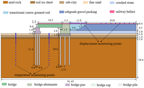
Figure 1.
Embankment–bridge transition zone model diagram (Unit: m).
3.1.2. Model Meshing of Transition Zone
The COMSOL Multiphysics software is a numerical simulation software based on finite elements, which has powerful abilities in multi-physics coupling and solving nonlinear differential equations. The hydrothermal and frost heave characteristics model of the embankment–bridge transition zone are simulated by the coefficient type partial differential equation PDE module of COMSOL Multiphysics. Considering that the numerical model of the embankment–bridge transition zone is relatively complex, the mesh in some regions that need to be analyzed is encrypted, and the mesh is set in the vertical and horizontal directions with a gradually sparse transition mode for distant areas. In addition, the mesh density should be adjusted according to the needs of calculation accuracy, cost, and convergence during the calculation process.
3.1.3. Calculation Parameter
- a.
- Hydrothermal parameters of soil layer
Hydrothermal parameters include thermal physical parameters and water field parameters. Thermal physical parameters of materials are important internal factors for solving the temperature field of frozen embankments in the embankment–bridge transition zone. Thermal conductivity, specific heat capacity, and latent heat of phase transition of various materials under different freeze–thaw conditions should be determined. The above parameters are affected by factors such as material characteristics, density, and water content, and should usually be measured. However, due to the spatial heterogeneity and time variability of soil property parameters in permafrost, the testing workload and difficulty are relatively large. Therefore, the thermal physical parameters and water field parameters of various materials in the numerical model of the embankment–bridge transition zone in this paper mainly refer to existing studies [27,28,29,30,31,32,33,34,35], and the specific values are summarized in Table 1, Table 2 and Table 3.

Table 1.
Hydrothermal parameters (, , , ) [28,29,32,33,35].
Table 2.
Hydrothermal parameters (, , , ) [28,29,32,33,35].
Table 3.
Hydrothermal parameters (, , , ) [28,29,32,33,35].
- b.
- Mechanical parameters of soil layer
Since the mechanical properties of frozen soil change with changes in temperature, the mechanical parameters of each medium in the calculation model will be different as the temperature changes. The relationship between the elastic modulus and Poisson’s ratio of frozen soil body and soil temperature can be expressed by the following formula [33], and the specific values are summarized in Table 4:
where E is the elastic modulus (MPa); ν is the Poisson’s ratio; ai and bi are the test coefficients, i = 1, 2 …; and m is the nonlinear index, usually with a value of 0.6.
Table 4.
Mechanical parameters [28,29,31,32].
- c.
- Bridge and pier system parameters
Considering that the bridge and abutment are both concrete structures, the specific heat and thermal conductivity of the bridge are the same. The pier has little influence on the result, so all parameters of the pier are consistent with those of the bridge. The physical mechanics and thermal parameters of the pile foundation system of bridge piers are summarized in Table 5.
Table 5.
Physical mechanics and thermal parameters of concrete construction [36,37].
3.1.4. Boundary Conditions
- a.
- Upper surface boundary
Based on the boundary layer principle and the long-term monitoring data in the Qinghai–Tibet region, it can be assumed that the upper boundary condition of the model is the temperature boundary condition [38]. In addition, the upper boundary condition of the calculation region can be simplified into a trigonometric function form, and the time when the temperature boundary temperature is the highest is taken as the starting calculation time (that is, the upper boundary temperature is assumed to be 15 July) [30]. The temperature variation of the upper boundary between the embankment surface and the natural surface is described by functions (16) and (17). It should be noted that the temperature boundary is an empirical expression based on long-term monitoring data.
The surface temperature boundary of the abutment structure is about 1.5 °C lower than that of the top surface of the embankment [28], so the surface temperature of the bridge-pier abutment can be as follows:
- b.
- Other boundary conditions
The bottom boundary of the model fixed horizontal and vertical displacement and angular freedom at the same time, and the left and right sides of the model only fixed horizontal freedom and allowed vertical free deformation. Tangential and normal contacts are considered between the abutment back and the filler. At the same time, the relative movement between abutment and cap, pier, and foundation soil is ignored.
3.2. Analysis of Temperature Field Calculation Results
Using the above analysis method, the theoretical formula is embedded into the model through the PDE module of the COMSOL software, and a freeze–thaw period is calculated with a starting date of 15 July 2023. This section will analyze the temperature field results of the embankment–bridge transition zone during the freeze–thaw period.
3.2.1. Analysis of Temperature Field Prediction Results
In this section, 15 July and 15 January are considered as the highest and lowest temperatures in a year, respectively, 15 July 2023 is regarded as the initial moment of the freeze–thaw cycle, and the temperature field distribution until 15 July of the following year is predicted. The calculation results of the temperature field are shown in Figure 2.
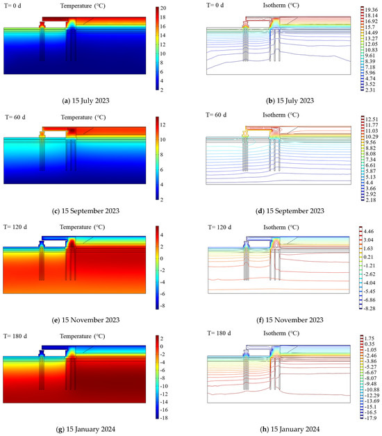
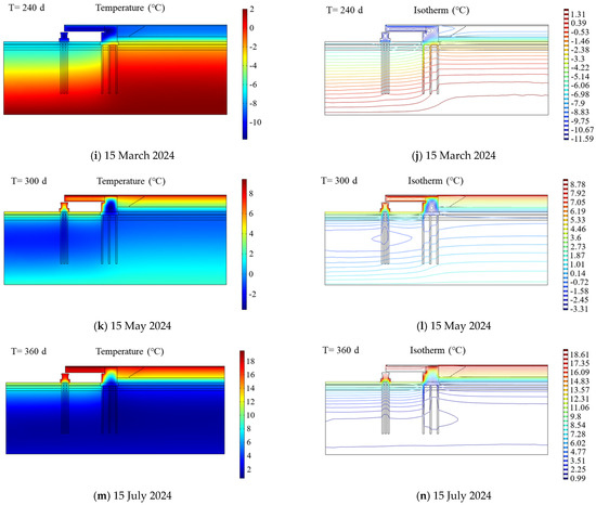
Figure 2.
Temperature of the embankment–bridge transition zone from mid–July 2023 to mid–July 2024.
As can be seen from the temperature cloud diagram and isotherm diagram for 15 July to 15 September, the highest temperature is mainly concentrated in the bridge-pier abutment structure, because the material of these structures is concrete, which has better thermal conductivity than the filler and natural soil behind the abutment, and can promote the heat exchange with the outside air temperature more quickly. In addition, it can be observed that the isotherm of soil filled behind the abutment near the abutment is more irregular and fluctuates more violently than the isotherm at positions farther away from the abutment, indicating that the abutment at the embankment–bridge transition zone in cold regions has a certain influence on the temperature field distribution.
The lowest temperatures during the period from November 2023 to March 2024 are located in bridge and pier structures, due to the lower atmospheric temperature compared to the bottom boundary during this period and the faster heat conduction of concrete structures. At this stage, a hot interlayer can be observed in the middle of the bridge. The existence of a hot interlayer indicates that there is a large area of the high-temperature area in the backfill of the bridge transition zone. Therefore, under the long-term load of freeze–thaw environments and train vibrations, the settlement of the backfill behind the bridge transition zone will be much larger than that of the abutment, thus producing differential settlement and adversely affecting the stability of the transition zone.
From the temperature cloud map and isotherm chart from March 2024 to July 2024, it can be seen that the highest temperature is mainly distributed in the upper part of the bridge structure, which is because the external temperature has gradually increased since April. Due to the heat exchange and the redistribution of the temperature field, it is also observed that the cold interlayer is gradually transferred from the inside of the abutment to the inside of the backfill of the abutment, and the lowest temperature is gradually transferred from the inside of the abutment to the deep soil.
3.2.2. Comparison of Ground Temperature at Typical Monitoring Sites
In order to analyze the change in ground temperature in the embankment–bridge transition zone during the freeze–thaw period, monitoring points were set at different buried depths of the natural foundation under the bridge midpoint and 30 m away from the abutment. Figure 3 represents the time-history curve of ground temperature at typical monitoring points in shallow natural foundations and the time-history curve of typical monitoring points in deep natural foundations. In this section, the buried depth within 4 m from the surface or embankment surface is defined as shallow soil and the buried depth below 4 m from the surface or embankment surface is defined as deep soil.
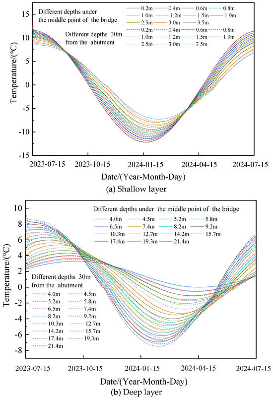
Figure 3.
Ground temperature time history of typical monitoring points of natural foundation.
It can be seen that the ground temperature at both shallow and deep monitoring points presents a sinusoidal distribution. That is, the ground temperature under the middle point of the bridge is slightly higher than the ground temperature 30 m away from the abutment, and the difference between the two will gradually increase with the increase in buried depth. The reason why the ground temperature under the bridge midpoint is slightly higher than the ground temperature 30 m away from the bridge abutment may be that the thermal conductivity of the concrete pile foundation under the bridge pier and bridge is better than that of the frozen soil, so it is more conducive to the heat exchange between the soil inside and the external environment.
It can be seen from the time-history curve of the ground temperature at typical monitoring points of natural foundation that the ground temperature at both shallow and deep monitoring points presents sinusoidal variation. In Figure 3, it can also be observed that there is a phase difference between the ground temperature time history curves of different buried depths in shallow and deep layers (phase hysteresis phenomenon). In addition, as the buried depth increases, the influence of the temperature boundary condition on the soil inside the numerical model gradually decreases, so the ground temperature amplitude gradually decreases.
3.3. Analysis of Water Field Calculation Results
The main purpose of water field simulation is to analyze the distribution of solid ice and the frost heave deformation of the embankment–bridge transition zone. From July 2023 to July of the following year, the water field and solid ice distribution in the transition zone are shown in Figure 4. The surface layer of ballast is filled with graded gravel, so the initial moisture content is set to 1.2%, the initial moisture content of coarse grain soil and embankment gravel filler is set to 5%, and the initial moisture content of natural formation is set to 10%. Concrete structures such as abutments do not participate in the calculation of the water field.
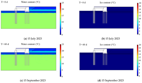
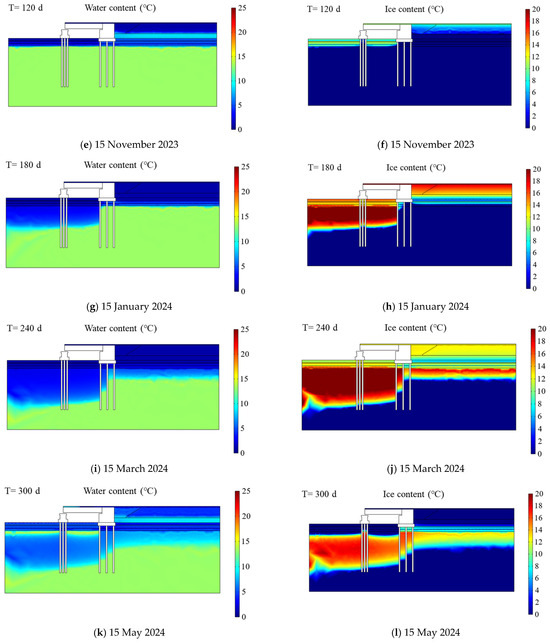
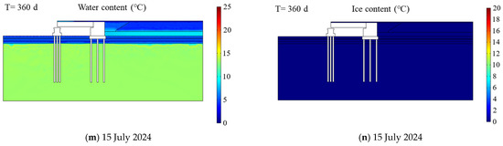
Figure 4.
Water in the embankment–bridge transition zone from mid-July 2023 to mid–July 2024.
When the embankment fill starts to freeze behind the abutment, under the action of the soil matrix potential gradient, the water in the unfrozen region migrates and freezes continuously to the freezing front, resulting in an increase and downward migration of water content at the freezing front and a drastic change of water content near the front. Water migrates to the road surface under the action of matrix suction, and with the increase in freezing depth, the surface of the embankment is frozen. In mid-December, the natural soil layer behind the abutment began to freeze, and there was a lag effect compared with the freezing time of the natural soil layer in front of the abutment.
From the middle of April of the next year, the surface soil began to melt. During the melting process, the water accumulated in the frozen soil layer melted and migrated downward under the action of gravity potential gradient, resulting in a peak water content area at the melting front. During the whole process, water content and ice content show the opposite trend, and due to the influence of the structure of the abutment, there are some differences in the freezing and melting characteristics of the natural soil layer before and after the abutment.
3.4. Analysis of Frost Heave Deformation Calculation Results
3.4.1. Vertical Frost Heave of Ballast Surface
In this section, only one frost heave condition is considered, where the initial moisture content of both the transition zone fill and embankment fill is 5%. Frost heave is assumed to start from 15 October, and the calculation results are shown in Figure 5.
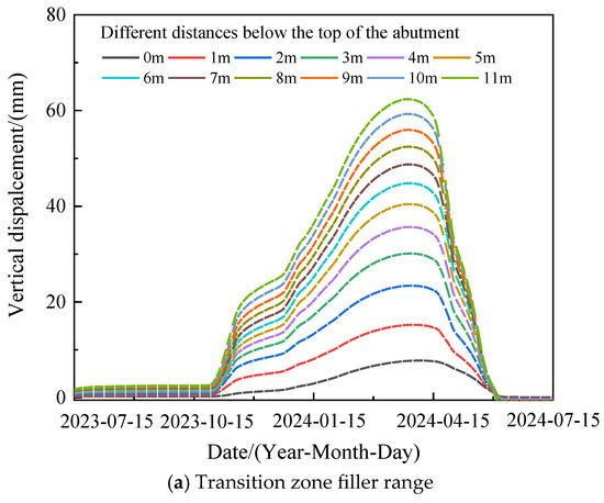

Figure 5.
Vertical frost heave time history of typical monitoring points behind the abutment.
Figure 5 shows the vertical frost heaving time history of the ballast surface in the packing range of the transition zone behind the abutment and in the packing range of the embankment, respectively. On the whole, with the decrease in temperature in the freezing period, the soil mass experiences frost heave due to the phase transition of ice water, and the frost heave value of the ballast surface reaches the peak in April of the following year. In the spring thaw period, the soil mass causes thaw subsidence due to the rise of temperature, and the displacement of the ballast surface gradually decreases. In the filler range of the transition zone behind the abutment, the vertical frost heave amplitude decreases as the distance from the abutment back increases, and the minimum is 8 mm. In the range of 0–5 m, the frost heave amplitude increases rapidly as the distance from the abutment back increases, while in the range of 5–11 m from the abutment back, the frost heave amplitude increases slightly slowly. However, in the embankment filler range, that is, 20–40 m behind the embankment abutment, the frost heave curve almost overlaps, and the difference in frost heave amplitude does not exceed 5 mm. It can be seen from the analysis that the influence of abutment structure on the vertical frost heave of the backfill is mainly concentrated in the range of the transition zone, and the vertical frost heave near the abutment is much smaller than the other parts far away from the abutment, indicating that the longitudinal binding force of the abutment on the backfill is much smaller than the horizontal frost heave force of the fill. Therefore, the total frost heave deformation of the filler is more in the form of horizontal frost heave, which limits the development of vertical frost heave.
3.4.2. Horizontal Frost Heave of the Backfill behind Abutment
In this model, it is assumed that the initial calculation state of the embankment–bridge transition zone is that the contact force and contact area between the backfill and the abutment are “0”, and the two will contact in the process of gradually being subjected to the horizontal frost heave force of the backfill behind the abutment. According to the analysis of Figure 6 and Figure 7, it can be seen that the freeze-heave of the backfill began to increase slowly in mid-to-late October, and the abutment gradually began to contact the backfill of the abutment under the horizontal freeze-heave of the backfill of the abutment. The contact force of the abutment and the backfill of the abutment rapidly reached the maximum and stabilized in early November, during which the backfill and the abutment were in a state of “complete contact”. The contact force between the backfill and the abutment also developed rapidly and reached its peak around the end of March. After the end of March, with the decrease in frost heave deformation, the contact force and contact area between the backfill and the abutment gradually decreased.

Figure 6.
Change trend of contact force between backfill and abutment.
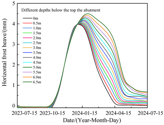
Figure 7.
Variation of horizontal frost heave deformation at different positions of abutment back.
3.4.3. Bridge–Abutment Interaction
In the calculation process of this model, the “extrusion” phenomenon of bridge–abutment encountered in actual engineering was observed, as shown in Figure 8. With the development of frost heave on the backside of the platform, the frost heave force on the abutment increases, and the abutment moves sideways and tilts toward the bridge. The contact force between the abutment and the abutment also increases with the development of frost heave until it reaches its peak value around mid-March. By comparing the peak value of the contact force between the backside of the abutment and the abutment, it can be found that the two are in the same order of magnitude and cannot be ignored. Therefore, the frost heaving of the backfill will not only cause abutment diseases but also lead to a series of additional bridge structural diseases. It is suggested that the moisture content of the backfill should be strictly controlled during the construction of the embankment–bridge transition zone in cold regions to limit the horizontal frost heaving deformation of the abutment.
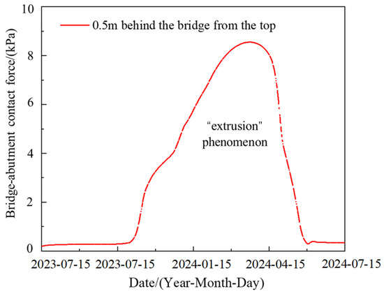
Figure 8.
Change of bridge–abutment contact force.
4. Dynamic Characteristics Analysis of Train-Track-Embankment–Bridge Transition Zone under Frost Heave Conditions
4.1. Numerical Model
The irregular vertical deformation of track structures occurs under the action of frost heave in the transition zone filler, and the dynamic response of these track irregularity areas will be significantly amplified under the action of train loads. In order to analyze the dynamic response of embankment–bridge transition zones under the condition of track deformation caused by the freeze-heave action of fillers behind abutments, a finite element dynamic model of the train-rail-embankment–bridge transition zone was established. This model considers the combined action of freeze-heave deformation and train vibration load by using ABAQUS software (Das-sault Systemes), as shown in Figure 9, based on the finite element method and the coupling dynamics theory of vehicle-track, and introduces wheel–rail interaction [36,39,40,41,42]. In addition to the train, rail, and sleeper, the under-rail structure of the dynamics model of the train-rail-bridge transition zone is consistent with the dimensions of the above hydrothermal model of the transition zone. The parameters of the train and track model are shown in Table 6. In addition, the elastic modulus, Poisson’s ratio, and density of the steel rail are 2.059 × 10⁵ MPa, 0.3, 7800 kg/m3, respectively. The elastic modulus, Poisson’s ratio, and density of the train sleeper are 3.75 × 10⁴ MPa, 0.3, and 2600 kg/m3, respectively [36,37,40,41,42,43,44,45]. The actual frost heave deformation of the upper surface of the ballast obtained by hydrothermal analysis is applied to the dynamic model as the initial condition, then the dynamic load of the train and track structure is applied, and the dynamic response of the transition zone structure under frost heave conditions is obtained.

Figure 9.
Finite element dynamic model of railway train-track-embankment–bridge transition zone considering frost heave deformation.
Table 6.
Train and rail parameters [36,37,40,41,42,43,44,45].
4.2. Comparison of Calculation Results under Frost Heave and Non-Frost Heave Conditions
As mentioned above, the frost heave deformation reaches its maximum value around mid-March. Therefore, the calculated frost heave deformation on 15 March of the following year is applied to the upper surface of the ballast in the dynamic model as the initial condition, the dynamic response under frost heave condition is analyzed, and the difference between the dynamic response of the transition zone under frost heave condition and non-frost heave condition is compared. The train speed is set at a moderate 120 km/h. The surface of the transition zone filler at 0 m/4 m/8 m behind the abutment and the surface of the embankment filler at 12 m/16 m behind the abutment were taken as monitoring points to analyze the vertical acceleration, vertical dynamic stress, and vertical dynamic deformation of transition zone filler and embankment filler surfaces at different distances from the back of the abutment under frost heave and non-frost heave conditions.
4.2.1. Acceleration
It can be observed from Figure 10 that the acceleration amplitude is located 0 m behind the abutment in the condition of non-frost heave and 8 m behind the abutment in the condition of frost heave, and the acceleration amplitude in the condition of frost heave (9.79 m/s2) is much higher than that in the condition of non-frost heave (3.50 m/s2). The acceleration response time history is fuller in the condition of non-frost heave, while the acceleration amplitude increases significantly in the condition of frost heave, which may be due to the increased wheel–rail interaction caused by irregular train bounce and wheel–rail impact. Under non-frost heave conditions, the acceleration amplitude decreases with the increase in the distance from the back of the abutment, and the change of acceleration amplitude under frost heave conditions has no close correlation with the distance from the back of the abutment, indicating that the acceleration response under non-frost heave conditions is mainly affected by the stiffness difference of the transition segment, while under frost heave conditions, it is mainly affected by frost heave deformation.
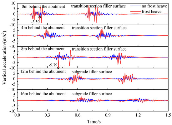
Figure 10.
The vertical acceleration time history of different monitoring points on the filler surface at different distances from the back of the abutment.
4.2.2. Dynamic Stress
It can be observed from Figure 11 that the maximum value under non-frost heave conditions is located at 4 m behind the abutment, and the dynamic stress amplitude within 4~16 m behind the abutment exceeds 80 kPa with little difference, which is much larger than the dynamic stress amplitude at 0 m behind the abutment. Under frost heave conditions, the maximum value is located at 0 m behind the abutment, and the dynamic amplitude of different distances behind the abutment is different and smaller than the dynamic stress amplitude at 0 m behind the abutment. The maximum dynamic stress amplitude under frost heave conditions (204.12 kPa) is about 2.4 times that under non-frost heave conditions (84.63 kPa). The irregular distribution of dynamic stress amplitude under different distances from the abutment is mainly affected by the random bouncing of trains and wheel–rail impact. The dynamic stress time history curve under the condition of non-frost heave presents a double “W” shape, with each wheelset corresponding to a peak value and little difference between each peak value. Meanwhile, the dynamic stress time history under the condition of frost heave presents a double “W” shape, a double “V” shape, or a mixed “W-V” shape, with certain differences between each peak value. As a whole, the peaks corresponding to the two wheelsets of the first bogie are larger than those of the second bogie. The “W” type indicates that the four wheelsets of the corresponding section are in contact with the track when the train runs, and the “V” type indicates that there may be wheel–rail separation during the train operation.
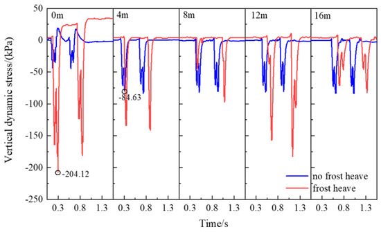
Figure 11.
The dynamic stress time history of different monitoring points on the filler surface at different distances from the back of the abutment.
4.2.3. Dynamic Deformation
It can be observed from Figure 12 that there are great differences in dynamic deformation rules between non-frost heave conditions and frost heave conditions. The dynamic deformation time history of non-frost heave conditions all present a “W” shape, while the dynamic deformation time history curves of transition zone/embankment filler surface at different distances from the back of the abutment under frost heave conditions are chaotic and irregular due to the influence of irregular train bounce and wheel–rail impact. Under non-frost heave conditions, the vertical dynamic deformation amplitude of different section surfaces behind the abutment has little difference, and the maximum value is located at 4 m behind the abutment. Under frost heave conditions, the vertical dynamic deformation amplitude at different distance sections behind the abutment is significantly different. The maximum value (4.79 mm) is about 2.8 times that of the minimum value (1.71 mm), and the maximum and minimum values are located at 12 m and 0 m behind the abutment, respectively. The maximum value of vertical dynamic deformation under frost heave conditions is significantly greater than that under non-frost heave conditions. The vertical dynamic stress and dynamic displacement of the train will “return to zero” (tend to the initial state) before and after the train passes through the non-frost heave condition, and the abnormal phenomenon of dynamic stress and dynamic displacement near 0 m behind the abutment under the frost heave condition may be caused by the redistribution of stress and strain field when the train impacts the frost heave soil. Therefore, the stress–strain distribution after the passage of the train is different from the initial stress field and strain field.
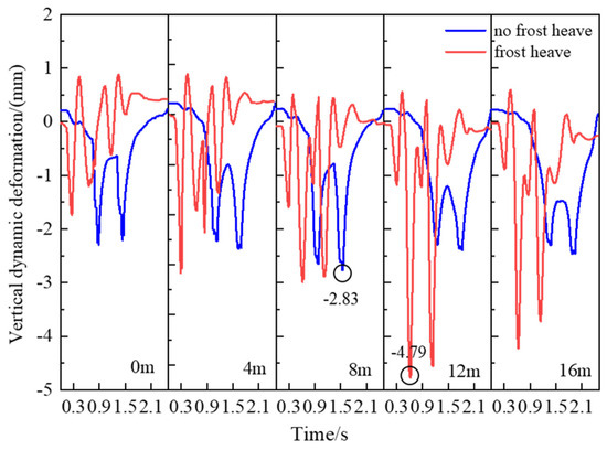
Figure 12.
The dynamic deformation time history of different monitoring points on the filler surface at different distances from the back of the abutment.
4.2.4. Wheel–Rail Contact Force
In the process of train operation, the vibrations caused by the interaction between the wheelset and the track are transmitted to the ballast and the soil below along the sleeper. The wheel–rail contact force plays an important role in the analysis of the dynamic response of the soil during the train operation, so the analysis of the wheel–rail contact force is very important.
It can be seen from Figure 13 that the time history of wheel–rail contact force between the first wheel and the last wheel of the train is very regular without considering frost heave. The wheel–rail contact force of the first wheel and the last wheel of the train both fluctuate relatively stably around 75 kN. The time history of the contact force between the first wheel and the last wheel of the train fluctuates greatly under frost heaving conditions. When the train runs within the abutment range, the wheel–rail contact force of the first wheel fluctuates slightly within the range of 75 kN. When the first round is near the filler of the transition zone, the wheel–rail contact force increases sharply and reaches the maximum wheel–rail contact force of 548.12 kN (the first peak value) near 0.175 s. Under the action of rail reaction in the first wheel, the wheel–rail contact force decreases sharply to close to 0 and then fluctuates, and a short wheel–rail detachment occurs (red in the figure represents the derailment risk area). After the first wheel falls back and continues to contact the rail, the contact force reaches the second wheel–rail contact force peak value of −385.03 kN in the fluctuating process. After the peak, the wheel–rail separation phenomenon was observed for a long time, the third wheel–rail contact force peak value of −334.56 kN was reached when the wheel–rail contact was made again within the embankment filler range of about 0.3 s after the holding time, and then the first wheel–rail contact force gradually stabilized after a short and violent fluctuation.
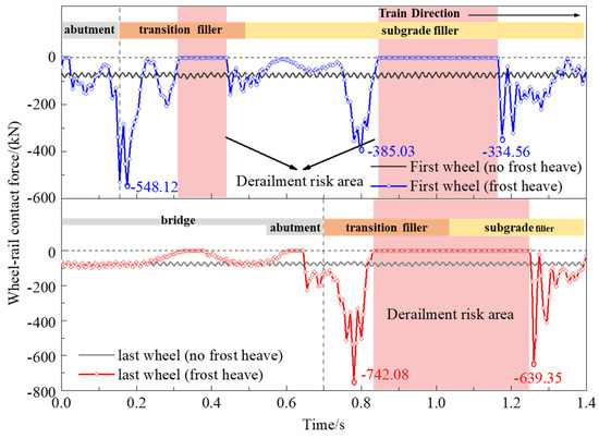
Figure 13.
Time history of wheel–rail contact force at embankment–bridge transition zone during train running under frost heave condition.
For the last wheel, when the train runs within the abutment range, the wheel–rail contact force of the last wheel fluctuates slightly within the range of 75 kN. It is worth noting that the wheel–rail contact force of the tail wheel decreases significantly when the train runs for 0.2~0.3 s, and this area corresponds exactly to the departure area of the first wheel of the wheel–rail. Therefore, this phenomenon may be caused by the impact of the first wheel in the range of the filler in the transition zone caused by the deformation of the rail caused by the frost heave of the filler. Similar to the first wheel, the wheel–rail contact force increases sharply when the tail wheel is near the filler of the transition zone, and reaches the maximum wheel–rail contact force of 742.08 kN (the first peak value) near 0.78 s. The last wheel bounces off the rail under the action of huge reverse force, and the derailments take up to 0.4 s. Then, it falls back and impacts the rail again within the range of the embankment filler to reach the second wheel–rail contact force peak of −639.35 kN.
The maximum peak value of the wheel–rail contact force of the first and last wheels under frost heaving conditions is much greater than that under non-frost-heaving conditions, indicating that the effect of frost heaving on wheel–rail contact force is great and cannot be ignored. In addition, it is also found that the maximum peak value of the wheel–rail contact force for the last wheel (−742.08 kN) is significantly greater than that of the first wheel rail contact force (−548.12 kN). This may be due to the fact that the wheel–rail contact force is not only affected by factors such as axle load, vertical deformation of the rail, and the form and stiffness of the structure under the rail, but also by the train’s running attitude. Although there is a large difference in the peak value of wheel–rail contact force between the first and last wheels, it can be found that the total derailment time of the first and last wheels is very small by comparing the red area in the figure. It can also be observed from the figure that the longer the derailment time, the greater the wheel–rail contact force when the wheel–rail contact again. Therefore, it is recommended to control the frost heave deformation of the filler and the train operating speed to reduce the derailment risk and minimize the wheel–rail contact force. It can also be found that the wheel–rail contact force is mainly affected by the stiffness difference of the transition zone under non-frost heave conditions, while there is no close correlation between the wheel–rail contact force change and the stiffness difference of the transition zone under frost heave conditions. The vertical geometric irregular deformation of the rail caused by vertical frost heave is the main factor that magnifies the dynamic response of the wheel–rail contact force.
5. Conclusions
In this study, the hydrothermal model and the dynamic analysis model of the embankment–bridge transition zone in cold regions were established, and the temperature field, water field, and frost heave deformation law of the transitional section were studied. The dynamic response and wheel–rail contact characteristics of the filler in the transition zone were compared and analyzed under the conditions of non-frost heave and frost heave. The following conclusions can be drawn from the results:
- (1)
- The isotherm of soil filled behind the abutment near the abutment is more irregular and fluctuates more violently than the isotherm at the position farther away from the abutment, indicating that the abutment at the embankment–bridge transition zone in cold regions has a certain influence on the temperature field distribution. The ground temperature of deep soil and shallow soil follows the laws of sinusoidal distribution, phase lag, and amplitude attenuation, and there are hot interlayers and cold interlayers. Due to the influence of the structure of the abutment, the freezing and melting characteristics of the natural soil layer before and after the abutment are different, and the freezing time of the natural soil layer behind the abutment has a lag effect.
- (2)
- The effect of the abutment structure on the vertical frost heave of filler is mainly concentrated in the range of the transition zone, and the vertical frost heave near the abutment is much smaller than other parts away from the abutment. The contact force between the backfill and the abutment developed rapidly from the end of October with the continuous development of the horizontal frost heave of the backfill and reached a peak value around the end of March of the next year. With the decrease in frost heave deformation, the contact force and contact area between the backfill and the abutment also gradually decreased. With the development of frost heave behind the abutment, the force of frost heave behind the abutment increases, and the phenomenon of “extrusion” of the abutment will occur in practical engineering.
- (3)
- There are obvious differences in the amplitude, distribution, and attenuation of dynamic response and wheel–rail contact force in the embankment–bridge transition zone under non-frost heave and frost heave conditions. Due to the increase in the wheel–rail interactions caused by irregular train bounce and wheel–rail collision, the acceleration response time under non-frost heave conditions is fuller, while the acceleration amplitude under frost heave conditions is significantly increased. Compared with the non-frost heave condition, there are significant differences between the peaks of the dynamic stress and the time history curve of the dynamic deformation under frost heave conditions.
- (4)
- Frost heave has a great influence on wheel–rail contact force. The larger the derailment risk area, the more significant the increase in wheel–rail contact force when the wheel–rail falls back to the track. Therefore, it is recommended to control the frost heave deformation of the filler and the train running speed to reduce the risk of derailment and minimize the wheel–rail contact force. The change in wheel–rail contact force under non-frost heave conditions is mainly affected by the stiffness difference in the transition zone, while the change in wheel–rail contact force under frost heave conditions is not closely related to the stiffness difference in the transition zone. The vertical geometric irregular deformation of rail caused by vertical frost heave is the main factor amplifying the dynamic response of wheel–rail contact force.
Author Contributions
Conceptualization, X.H.; Formal analysis, X.H.; Investigation, Y.W.; Methodology, X.H. and Y.W.; Project administration, L.D.; Software, X.H. and Y.W.; Supervision, S.T., L.D. and X.L.; Validation, X.H.; Writing—original draft, X.H.; Writing—review and editing, S.T. All authors have read and agreed to the published version of the manuscript.
Funding
This study was financially supported by the National Natural Science Foundation of China (Grant No. 42072316; Grant No. 42102311), Key Laboratory of Coal Gangue Resource Utilization and Energy-Saving Building Materials of Liaoning (Grant No. LNTUCEM-2304), and the Fellowship of China Postdoctoral Science Foundation (Grant No. 2021M701014).
Institutional Review Board Statement
Not applicable.
Informed Consent Statement
Not applicable.
Data Availability Statement
The data presented in this study are available from the corresponding author upon request.
Conflicts of Interest
Author Liang Dong was employed by the company Railway Engineering Research Institute, China Academy of Railway Sciences Corporation Limited, Beijing 100081, China. The remaining authors declare that the research was conducted in the absence of any commercial or financial relationships that could be construed as a potential conflict of interest.
References
- Harlan, R.L. Analysis of coupled heat-fluid transport in partially frozen soil. Water Resour. Res. 1973, 9, 1314–1323. [Google Scholar] [CrossRef]
- Taber, S. Frost heaving. J. Geol. 1929, 37, 428–461. [Google Scholar] [CrossRef]
- Miller, R.D. Frost heaving in non-colloidal soils. In Proceedings of the 3rd International Conference Permafrost, Edmonton, AB, Canada, 10–13 July 1978; National Research Council of Canada: Ottawa, ON, Canada, 1978. [Google Scholar]
- Gilpin, R.R. A model for the prediction of ice lensing and frost heave in soils. Water Resour. Res. 1980, 16, 918–930. [Google Scholar] [CrossRef]
- Sheng, D. Thermodynamics of Freezing Soils: Theory and Application. Ph.D. Thesis, Luleå Tekniska Universitet, Luleå, Sweden, 1994. [Google Scholar]
- Konrad, J.M.; Morgenstern, N.R. The segregation potential of a freezing soil. Can. Geotech. J. 1981, 18, 482–491. [Google Scholar] [CrossRef]
- Luo, X.; Ma, Q.; Niu, F.; Su, W.; Hu, H. Experimental and Numerical Analyses of Freezing Behavior of an Embankment in Cold Regions. Math. Probl. Eng. 2019, 2019, 1437904. [Google Scholar] [CrossRef]
- Yuan, C.; Niu, F.; Yu, Q.; Wang, X.; Guo, L.; You, Y. Numerical analysis of applying special pavements to solve the frost heave diseases of high-speed railway embankmentsin seasonally frozen ground regions. Sci. Cold Arid. Reg. 2018, 7, 340–347. [Google Scholar]
- Tai, B.; Liu, J.; Wang, T.; Shen, Y.; Li, X. Numerical modelling of anti-frost heave measures of high-speed railway embankment in cold regions. Cold Reg. Sci. Technol. 2017, 141, 28–35. [Google Scholar] [CrossRef]
- Zhang, Y.; Bei, J.; Li, P.; Liang, X. Numerical Simulation of the Thermal-Hydro-Mechanical Characteristics of High-Speed Railway Embankments in Seasonally Frozen Regions. Adv. Civ. Eng. 2020, 2020, 8849754. [Google Scholar]
- Ji, Y.; Zhou, G.; Vandeginste, V.; Zhou, Y. Thermal-hydraulic-mechanical coupling behavior and frost heave mitigation in freezing soil. Bull. Eng. Geol. Environ. 2021, 80, 2701–2713. [Google Scholar] [CrossRef]
- Lan, T.; Wang, J. Numerical Analysis of the Causes of Curved Soil Levee Breaches in Seasonal Freeze-Thaw Areas. KSCE J. Civ. Eng. 2020, 24, 2669–2681. [Google Scholar] [CrossRef]
- Xu, Q.; Peng, G.S.; Li, N.S.; Liu, Z. Numerical analysis of water-heat coupling in soil freezing process. J. Tongji Univ. (Nat. Sci. Ed.) 2005, 10, 5–9. (In Chinese) [Google Scholar]
- Shen, G.H. Influence of frost heave on the stress and deformation of ballastless track in transition zone. Chin. Railw. 2022, 3, 109–117. (In Chinese) [Google Scholar]
- Bian, X. Dynamic analyses of track and ground coupled system with high-speed train loads. Acta Mech. Sin. 2005, 37, 477–484. [Google Scholar]
- Hall, L. Simulations and analyses of train-induced ground vibrations in finite element models. Soil Dyn. Earthq. Eng. 2003, 23, 403–413. [Google Scholar] [CrossRef]
- O’brien, J.; Rizos, D.C. A 3D BEM-FEM methodology for simulation of high speed train induced vibrations. Soil Dyn. Earthq. Eng. 2005, 25, 289–301. [Google Scholar] [CrossRef]
- Zhai, W.M.; Song, E.X. 3D FEM in moving coordinate for transient response under moving loads. Rock Soil Mech. 2009, 30, 2830–2836. [Google Scholar]
- Ai, Z.Y.; Mu, J.J.; Ren, G.P. 3D dynamic response of a transversely isotropic multilayered medium subjected to a moving load. Int. J. Numer. Anal. Methods Géoméch. 2018, 42, 636–654. [Google Scholar] [CrossRef]
- Zhu, Z.-y.; Ling, X.-z.; Chen, S.-j.; Zhang, F.; Wang, Z.-y.; Wang, L.-n.; Zou, Z.-y. Analysis of dynamic compressive stress induced by passing trains in permafrost embankment along Qinghai–Tibet Railway. Cold Reg. Sci. Technol. 2011, 65, 465–473. [Google Scholar] [CrossRef]
- Chen, T.; Ma, W.; Wu, Z.-J.; Mu, Y.-h. Characteristics of dynamic response of the active layer beneath embankment in permafrost regions along the Qinghai-Tibet Railroad. Cold Reg. Sci. Technol. 2014, 98, 1–7. [Google Scholar] [CrossRef]
- Wang, Z.; Tian, L. Research on the Influence of Train Formation on the vibration Stress of Railway Embankment in Seasonally Frozen Region. IOP Conf. Ser. Earth Environ. Sci. 2019, 242, 032064. [Google Scholar]
- Wang, Z.; Ling, X.; Zhao, Y.; Zhang, F.; Tian, L. Numerical simulation of vibrational response characteristics of railway embankments with insulation boards. Sci. Cold Arid. Reg. 2022, 14, 23–31. [Google Scholar]
- Taylor, G.S.; Luthin, J.N. A model for coupled heat and moisture transfer during soil freezing. Can. Geotech. J. 1978, 15, 548–555. [Google Scholar] [CrossRef]
- Ning, L.; William, J.L. Unsaturated Soil Mechanics; Higher Education Press: Beijing, China, 2012. (In Chinese) [Google Scholar]
- Bai, Q.B. Boundary Layer Parameter Calibration and Numerical Simulation Method for Hydrothermal Stability of Frozen Embankment. Ph.D. Thesis, Beijing Jiaotong University, Beijing, China, 2018. (In Chinese). [Google Scholar]
- Xu, X.Z.; Deng, Y.S. Experimental Study on Water Migration in Frozen Soil; Science Press: Beijing, China, 1991. (In Chinese) [Google Scholar]
- Yin, Q.X. Study on the Spatial Temperature Field and Deformation Evolution Characteristics of Transition Zone of Road and Bridge in Permafrost Region. Ph.D. Thesis, China University of Mining and Technology, Xuzhou, China, 2015. (In Chinese). [Google Scholar]
- Tang, L.; Kong, X.; Li, S.; Ling, X.; Ye, Y.; Tian, S. A preliminary investigation of vibration mitigation technique for the high-speed railway in seasonally frozen regions. Soil Dyn. Earthq. Eng. 2019, 127, 105841. [Google Scholar] [CrossRef]
- Chen, S.J. Vibration Response of Trains Running on the Qingzang Line Embankment with Melted Interlayer and Underground Frozen Soil. Ph.D. Thesis, Harbin Institute of Technology, Harbin, China, 2013. (In Chinese). [Google Scholar]
- Ma, Z.T. Numerical Simulation of Thermal-Dynamic Response of Gravel Embankment in Permafrost Block. Ph.D. Thesis, Lanzhou University, Lanzhou, China, 2019. (In Chinese). [Google Scholar]
- Chen, X.J. Study on Differential Settlement and Treatment Measures of Transition Zone of Road and Bridge in Permafrost Area. Ph.D. Thesis, Xi’an University of Science and Technology, Xi’an, China, 2018. (In Chinese). [Google Scholar]
- Li, S.Y. Numerical Simulation of Thermal-Mechanical Stability of Railway Embankment in Permafrost Area; Cold and Arid Regions Environmental and Engineering Research Institute, Chinese Academy of Sciences: Beijing, China, 2008. [Google Scholar]
- Ma, W.; Wang, D.Y. Mechanics of Frozen Soil; Science Press: Beijing, China, 2014; pp. 273–276. [Google Scholar]
- Zhang, M.L.; Wen, Z.; Xue, K.; Chen, L.; Li, D.; Gao, Q. Analysis of temperature and deformation of slope embankment in wetted section of permafrost area of Qinghai-Tibet Railway. Chin. J. Rock Mech. Eng. 2016, 35, 1677–1687. (In Chinese) [Google Scholar]
- Dong, L.; Wu, Y.K.; Zou, J.A.; Han, X.; Su, Y.H. Numerical simulation of frost heave characteristics of railway bridge transition section in high-cold seasonal frozen soil region. Chin. J. Railw. Sci. 2024, 45, 68–78. (In Chinese) [Google Scholar]
- Wu, Z.L. Influence Analysis and Dynamic Response of Frost Heave on Track Irregularity of High-Speed Railway Embankment. Master’s Thesis, Beijing Jiaotong University, Beijing, China, 2015. (In Chinese). [Google Scholar]
- Wang, L.N. Embankment Vibration Response and Cumulative Permanent Deformation of Train Running in Permafrost Area of Qinghai-Tibet Railway. Ph.D. Thesis, Harbin Institute of Technology, Harbin, China, 2013. (In Chinese). [Google Scholar]
- Wu, Y.K. Dynamic Response Characteristic Analysis of Frost Heaved Bridge Transition Zone of Sichuan-Tibet Railway. Master’s Thesis, Harbin Institute of Technology, Harbin, China, 2022. (In Chinese). [Google Scholar]
- Tian, S. Analysis of Mechanical Properties and Embankment Vibration Response of Coarse-Grained Filler in High Railway Foundation in High Cold Freeze-Thaw Area. Ph.D. Thesis, Harbin Institute of Technology, Harbin, China, 2020. (In Chinese). [Google Scholar]
- Dong, L.; Zhao, C.G.; Cai, D.G.; Zhang, Q.L.; Ye, Y.S. Numerical simulation and experimental study on dynamic characteristics of ballastless track subgrade of high-speed railway. J. Civ. Eng. 2008, 10, 81–86. (In Chinese) [Google Scholar]
- Dong, L.; Cai, D.G.; Ye, Y.S.; Zhang, Q.L.; Zhao, C.G. Cumulative deformation prediction method of high-speed railway subgrade under cyclic train load. J. Civ. Eng. 2010, 43, 100–108. (In Chinese) [Google Scholar]
- Guo, J. Influence of Uneven Embankment Settlement on Train Operation Safety and Track Dynamic Performance. Ph.D. Thesis, Beijing Jiaotong University, Beijing, China, 2017. (In Chinese). [Google Scholar]
- Luo, T. Study on Structural Mechanical Characteristics of Transition Zone of Sheet Pile Road Bridge in Permafrost Area. Ph.D. Thesis, Lanzhou Jiaotong University, Lanzhou, China, 2020. (In Chinese). [Google Scholar]
- Hao, J.F. Research on Track Dynamic Characteristics Analysis and Optimization Design of Transition Zone of High-Speed Railway. Ph.D. Thesis, Beijing Jiaotong University, Beijing, China, 2015. (In Chinese). [Google Scholar]
Disclaimer/Publisher’s Note: The statements, opinions and data contained in all publications are solely those of the individual author(s) and contributor(s) and not of MDPI and/or the editor(s). MDPI and/or the editor(s) disclaim responsibility for any injury to people or property resulting from any ideas, methods, instructions or products referred to in the content. |
© 2024 by the authors. Licensee MDPI, Basel, Switzerland. This article is an open access article distributed under the terms and conditions of the Creative Commons Attribution (CC BY) license (https://creativecommons.org/licenses/by/4.0/).