A Short-Term Vessel Traffic Flow Prediction Based on a DBO-LSTM Model

Abstract

To facilitate the efficient prediction and intelligent analysis of ship traffic information, a short-term ship traffic flow prediction method based on the dung beetle optimizer (DBO)-optimized long short-term memory networks (LSTM) is proposed. Firstly, according to the characteristics of vessel traffic flow, speed, and density, the traffic flow parameters are extracted from the AIS data; secondly, the DBO-LSTM model is established, and the optimal hyperparameter combinations of the LSTM are found using the DBO algorithm to improve the model prediction accuracy; then, taking the AIS data of a part of the coastal port area in Xiangshan as an example, we compare and analyze the results of the recurrent neural network, temporal convolutional network, LSTM, and DBO-LSTM prediction models; finally, the results are displayed and analyzed by visualization. The experimental results show that each error is reduced in predicting the flow parameter, speed parameter, and density parameter, and the accuracy reaches 95%, 92%, and 95%, respectively. After predicting the three parameters in the next 24 h, the accuracy rate reaches 93%, 91%, and 94%, respectively, compared with the real data, which surpasses the comparison model and achieves better prediction accuracy, verifying the feasibility and reasonableness of the proposed prediction model.

1. Introduction

As ports expand and global trade intensifies, the density of vessel traffic flows in ports and waterways escalates, potentially leading to severe congestion. Ship traffic congestion undermines the efficiency of maritime transportation and poses significant risks to navigational safety. Therefore, ensuring accurate traffic flow prediction is crucial for formulating systematic vessel entry plans and achieving efficient vessel traffic organization. Numerous scholars at home and abroad have focused their research on vessel traffic flow prediction. Vessel traffic flow prediction methods can be divided into two main categories:

First, the traditional method of predicting vessel traffic flow based on statistical models involves the use of mathematical statistical methods and theories to analyze known data and predict future trends. Its main components include Kalman filtering, gray scale prediction, Markov chains, and so on. Cai et al. developed a noise-immune Kalman filter for short-term traffic flow prediction, and the method showed higher prediction accuracy and stability under noisy data [1]. He et al. proposed an improved Kalman model that combines a regression analysis method and Kalman filtering for the short-term prediction of vessel traffic flow, which performs efficiently in capturing data with highly stochastic and nonlinear features [2]. Xiao and Duan propose a new gray model for traffic mechanics that has high prediction accuracy for uncertain data, but its applicability under extreme traffic conditions needs to be further investigated [3]. Ahn et al. used support vector regression and Bayesian classifiers to predict highway traffic flow, and experiments showed that this mixed-model approach performs well in complex and variable traffic flow situations [4]. Williams and Hoel used a seasonal autoregressive integrated moving average (ARIMA) model to predict traffic flow, which can effectively capture the seasonality and stochasticity in traffic flow [5]. Yin et al. used a fuzzy neural approach to predict urban traffic flow. The fuzzy logic system deals with the uncertainty of the input data through fuzzy rules and fuzzy reasoning, while the neural network is used to capture the complex nonlinear relationships in the data, and the proposed fuzzy neural network model exhibits high accuracy and reliability in urban traffic flow prediction [6]. Tian et al. used a new weighted least squares method to construct a basic graphical model of vessel traffic flow to solve the outlier problem of the traditional least squares method when dealing with noisy data [7]. However, traditional prediction models suffer from low prediction accuracy and robustness due to the influence of multiple factors on the actual vessel traffic flow. Due to the complexity of the nonlinear relationships involved, traditional vessel traffic flow prediction methods struggle to meet today’s real-time traffic control requirements.

Second, the vessel traffic flow prediction method based on machine learning includes machine learning theory and traffic flow prediction. It mainly includes traditional machine learning prediction methods such as support vector machine (SVM), random forest, and hidden Markov model, as well as deep learning prediction methods such as convolutional neural network (CNN), recurrent neural network (RNN) and others. Zhao et al. optimized a hidden Markov model to better fit the traffic flow at urban road intersections, and the optimized Markov model was able to more accurately capture the changing patterns of traffic flow [8]. Zhang et al. proposed a seasonal SARIMA and SVM model for predicting short-term traffic flow on highways. The SARIMA model performs well in dealing with data with obvious seasonality and trend, and the SVM model has advantages in capturing complex nonlinear relationship data, which combines the strengths of the two models and further improves the accuracy of traffic flow prediction [9]. Liu and Wu use the random forest algorithm to construct a traffic congestion state prediction model, which can effectively capture the changing trend of traffic flow and has significant advantages in prediction accuracy and generalization ability [10]. Koochali et al. used generative adversarial networks (ForGAN) for the probabilistic prediction of perceptual data. The ForGAN network outperformed traditional methods on several real-world perceptual datasets, and especially excelled in capturing the uncertainty of the data, making ForGAN a promising application in tasks that need to handle complex and uncertain time series prediction tasks, which makes ForGAN have a high potential for application [11]. Cai et al. proposed a noise-resistant long short-term memory network (LSTM) to predict short-term traffic flow, and added a noise-filtering mechanism in the model training to improve the prediction accuracy and robustness. However, the generalization ability of the model in different traffic environments needs to be further verified, especially for urban traffic flow prediction with different traffic patterns and structures [12]. Zhao et al. proposed a traffic flow prediction model called CHS-LSTM, but traffic patterns may vary significantly in different regions, and more empirical studies are needed for the model’s adaptability and robustness in these scenarios [13]. Ma et al. proposed a contextual convolutional recurrent neural network model that effectively captures the spatiotemporal characteristics of traffic data and improves the prediction accuracy by learning the intra-day and inter-day patterns of traffic flow, taking into account the influence of daily historical data on each other [14]. Fang et al. developed an error-free distributed long- and short-term memory network for short-term traffic flow prediction by relaxing the prediction error distribution of each iteration to an arbitrary distribution of long- and short-term memories to address the dependence of traditional methods on the error distribution assumption [15]. Yu proposed a master–slave structured particle swarm optimization (PSO) algorithm to train fuzzy wavelet neural networks (FWNNs) for short-term traffic flow prediction using a master–slave PSO algorithm, where the master swarm is responsible for the global search while the slave swarms perform the local search to optimize the parameters of FWNNs, which improves the efficiency and accuracy of the optimization [16]. Luo et al. proposed a KNN-LSTM short-term traffic flow prediction model based on K-nearest neighbor (KNN) and LSTM, which can utilize the temporal and spatial correlation characteristics of traffic flow to achieve highly accurate prediction, and improve the prediction accuracy by combining the KNN and LSTM to capture long-term dependencies in the time series [17]. Liu et al. proposed a multi-grouping LS-SVM method for urban short-term traffic flow prediction, but the process of data grouping needs to consider a variety of features and factors, and the choice of grouping strategy has an important impact on the prediction results, and overly complex grouping strategy may increase the complexity of model construction and training [18]. Qiao et al. constructed a one-dimensional CNN-LSTM neural network model for short-term traffic flow prediction, and the experiments show that the one-dimensional CNN-LSTM model outperforms the traditional single LSTM model and some other common methods, such as ARIMA and SVR, in terms of traffic flow prediction accuracy and stability [19]. Zhou, Wang proposed a novel ARIMA-LSTM model for multi-stage short-term traffic flow prediction, which assumes that the ARIMA model can fully capture the linear part of the data, while the LSTM model handles the nonlinear residuals, but in practice, linear and nonlinear data features may be intertwined, and this separate processing may miss some important features, affecting the prediction effect [20].

However, although the prediction tasks of urban traffic flow and ship traffic flow are similar in nature, they involve different environments and traffic conditions. In terms of environment and dynamic characteristics, the urban traffic flow environment is relatively fixed, the road network structure in the city is fixed, and the traffic flow has a significant time pattern, such as weekends and weekdays, daily morning and evening peak periods, and so on. The traffic flow also has the characteristics of high traffic density, affected by traffic signals and intersections and other complex traffic management factors. For the vessel traffic flow, its environment is more variable, including tides, currents, and other natural factors, and compared with the urban traffic flow is more dynamic. The sailing times and routes of ships are more uncertain, and also are affected by port scheduling and other factors, so compared with urban traffic, the time pattern of traffic flow is not as significant as that of urban traffic, and the density of traffic flow is also relatively low due to the large size of ships and slow travel speed. In terms of data characteristics, the data sources of urban traffic are extensive, which can be obtained from traffic sensors, GPS, traffic management systems, etc. [21], and the data update frequency is high, which can generate a large amount of data in a short period of time, and the types of data are also diverse, including vehicle type, traveling speed, lane occupancy, etc. The data sources of vessel traffic flow are more complicated than those of urban traffic, so the time pattern of traffic flow is not as significant as that of urban traffic. In contrast, the data source of vessel traffic flow is more concentrated, mainly relying on AIS data, port scheduling information, etc., and the frequency of data updating is low; the AIS data is usually updated at certain time intervals, such as a few minutes to a few tens of minutes. The type of data is also relatively simple, mainly including ship position, course, speed, and other information [22]. In terms of application scenarios and objectives, the purpose of urban traffic prediction tasks is mainly to optimize traffic management, improve traffic efficiency, and improve the traffic environment, which is mainly applied in intelligent transportation systems, navigation applications, and traffic planning [23]. The purpose of vessel traffic flow prediction tasks is mainly to optimize shipping routes, improve port operation efficiency, ensure navigation safety, etc., which is mainly applied in shipping company operation planning, the supervision and management of maritime related departments, and shipping risk assessment, etc. [24]. As can be seen above, urban traffic flow prediction and vessel traffic flow prediction have significant differences in data characteristics and application scenarios; understanding the differences between the two can lead to the better design and application of prediction models, so as to achieve better prediction accuracy and practical application results.

El Mekkaoui et al. propose a real-time prediction model that can be adapted to different routes and vessel types, and that captures the temporal and spatial characteristics of vessel speeds, in order to solve the problem of predicting vessel speeds in the St. Lawrence Seaway region [25]. Su et al. proposed an improved fuzzy neural network model for ship traffic prediction, which can adaptively adjust the fuzzy rules and network parameters to improve the prediction accuracy [26]. Tian and Qing proposed a gated recurrent unit (GRU) model combined with RNN to analyze multiple traffic flow sections in complex waters, which can effectively handle the complex spatial and temporal dependencies [27]. Hu et al. proposed a multimodal learning method P&G (Prophet and GRU) that can simultaneously learn the long-term and interdependence of multiple inputs while taking into account weather conditions for predicting vessel traffic flow [28]. Li et al. fused an improved CNN with LSTM to propose a temporal and spatial vessel traffic flow prediction model, but the method relies heavily on high-quality historical traffic data, which may affect the accuracy of the prediction results if the data are incomplete or noisy [29]. In recent years, deep learning prediction methods have shown promising prospects for development and application in the field of vessel traffic flow prediction. This is due to their ability to select data features through training and learning processes without manual intervention, leading to advantages such as strong generalization and adaptability.

Given the limited prediction accuracy and robustness of traditional statistical models, such as Kalman filter, gray scale prediction, and Markov chain, which render them inadequate for real-time ship traffic control due to the inherent challenges in solving nonlinear relationships, this paper adopts the deep learning method within the domain of machine learning prediction. However, while deep learning algorithms primarily focus on data decomposition to improve accuracy, the combination of hyperparameters in deep learning networks significantly affects the prediction results. Given the challenge of determining appropriate parameter combinations for diverse research data, multiple iterations for debugging become imperative. Therefore, the use of intelligent optimization algorithms to iteratively explore optimal parameter combinations in deep learning networks is crucial for improving prediction accuracy. As a result, an intelligent optimization algorithm is essential to iteratively fine-tune parameter combinations within deep learning networks to improve prediction accuracy. Zhang et al. used the adaptive particle swarm optimization (SAPSO) algorithm to adjust the structural parameters of the back-propagation neural network (BP) and proposed an improved PSO-BP model, called SAPSO-BP model, for the analysis and prediction of vessel traffic flow. The BP model, called the SAPSO-BP model, is used for the analysis and prediction of vessel traffic flow, and the experimental results show that this model outperforms the traditional other commonly used prediction models in the prediction of vessel traffic flow [30]. Qing, through experiments comparing the Griewank test function solving, found that the Dung Beetle Optimizer (DBO) algorithm has significant advantages over the Genetic Algorithm (GA), PSO, and Sparrow Search Algorithm (SSA) in terms of convergence speed, global optimum search, and optimization stability [31]. In this paper, an LSTM model optimized on the basis of the DBO algorithm is proposed and elaborated specifically for short-term ship traffic flow prediction. This combination is not only a simple integration of existing prediction methods, but also accurately optimizes the hyperparameters of the LSTM model through the efficient search capability of the DBO algorithm, thus significantly improving the prediction performance of the model, which has not been widely applied or thoroughly investigated in previous studies. Compared with the existing prediction models, we not only introduce DBO-LSTM to the task of ship traffic flow prediction, but more importantly, we precisely optimize the hyperparameters of LSTM by the DBO algorithm, which significantly improves the prediction accuracy and practicality, and at the same time provides important theoretical support and application value for port management and related decision making. The paper is organized as follows: Section 2 presents the theoretical foundations of the DBO algorithm and the LSTM model, as well as the construction of the combined model. Section 3 discusses the experiments and analyses performed. Finally, Section 4 presents the conclusion of the paper.

2. Materials and Methods

2.1. DBO Algorithm

In this study, we propose a kind of combinatorial model based on the DBO algorithm to optimize the LSTM model for short-term ship traffic flow prediction, which effectively finds the optimal hyperparameter combination of the LSTM through the global and local search mechanism of the DBO to improve the prediction accuracy and generalization ability of the model. The DBO algorithm is a new swarm intelligence optimization algorithm proposed by Professor Bo Shen’s team at Donghua University on 27 November 2022 [32]. In this context, each dung beetle position represents a solution, and the dung beetle population is classified into four groups based on their behavior: ball-rolling dung beetles, brood balls, small dung beetles, and thieving dung beetles. Throughout the iteration process, the positions of these four dung beetles are continuously updated as the solution evolves, ultimately resulting in the output of the global optimal position Xb and its corresponding fitness value. The process of updating their positions is as follows:

• Dung beetle roller

The ball-rolling dung beetle utilizes the sun as a guide to ensure that the dung ball rolls along a straight path. Its position update is depicted in Equations (1) and (2). In the event that the ball-rolling dung beetle encounters an obstacle hindering forward movement, it employs dancing behavior to adjust its direction. By utilizing the tangent function, it simulates a new rolling direction, and its dancing update position is represented by Equation (3).

$$x_i\left(m+1\right)=x_i\left(m\right)+a\times \mathrm{k}\times x_i\left(m+1\right)+\mathrm{b}\times \Delta x$$

(1)

$$\mathsf{\Delta }x=\left|x_i\left(m\right)-x^c\right|$$

(2)

$$x_i\left(m+1\right)=x_i\left(m\right)+tan\left(\theta \right)\left|x_i\left(m\right)-x_i\left(m-1\right)\right|$$

(3)

In the above equation, m represents the current number of iterations; x_i (m) denotes the position information of the ith dung beetle at the mth iteration; $\alpha$ is a natural coefficient assigned as −1 or 1 according to the probabilistic method, which is used to indicate whether or not it deviates from its original direction; k denotes the coefficient of deflection, which ranges between 0 and 0.2; b denotes a constant, which ranges between 0 and 1; $x^c$ denotes the global worst position; $\mathsf{\Delta }x$ is used to model the light intensity changes; $\mathsf{\theta }$ indicates the deflection angle, between 0~$\mathsf{\pi }$, and when equal to 0, $\mathsf{\pi }/2$, or $\mathsf{\pi }$, the position of the dung beetle is not updated. The values k and b are set to 0.1 and 0.3, respectively.

• Brooder ball

The brood balls were utilized within a boundary selection strategy to emulate the spawning area of female dung beetles. The spawning area was defined by Equations (4) and (5), while the position of the brood balls was determined by Equation (6).

$$L_b^{*}=\max \left(x^{*}\times \left(1-R\right),L_b\right)$$

(4)

$$U_b^{*}=\min \left(x^{*}\times (1+R),U_b\right)$$

(5)

$$B_i\left(m+1\right)=x^{*}+p_1\times \left(B_i\left(m\right)-L_b^{*}\right)+p_2\times \left(B_i\left(m\right)-U_b^{*}\right)$$

(6)

In the above equation, L_b^* and U_b^* represent the lower and upper limits of the spawning area, respectively; L_b and U_b represent the lower and upper bounds of the optimization problem, respectively; x* indicates the current local optimal position; R = 1 − m/m_max, m_max denotes the maximum number of iterations; B_i (m + 1) is the position information of the ith brood ball at time m; p₁ and p₂ denote two independent random vectors of size 1 × D. D denotes the dimension of the optimization problem.

• Little dung beetle

An optimal foraging area needs to be established to guide the hatchling dung beetle to find food and simulate its foraging behavior, where the optimal foraging area is defined as shown in Equations (7) and (8), and the position of the young dung beetle is updated as shown in Equation (9).

$$L_b^j=\max \left(x^j\times \left(1-R\right),L_b\right)$$

(7)

$$U_b^j=\min \left(x^j\times \left(1+R\right),U_b\right)$$

(8)

$$x_i\left(m+1\right)=x_i\left(m\right)+C_1\times \left(x_i\left(m\right)-L_b^j\right)+C_2\times \left(x_i\left(m\right)-U_b^j\right)$$

(9)

In the above equation, x_j denotes the current local optimal position; L_b^j and U_b^j denote the lower and upper limits of the optimal foraging area, respectively; x_i (m) denotes the location information of the ith small dung beetle at the mth iteration; C₁ denotes a random number that follows a normal distribution; C₂ denotes a random vector, between 0 and 1.

• Thief dung beetle

The thief dung beetle position is updated as shown in Equation (10).

$$x_i\left(m+1\right)=x^j+\mathrm{Q}\times g\times \left(\left|x_i\left(m\right)-x^{*}\right|+\left|x_i\left(m\right)-x^j\right|\right)$$

(10)

where xj is the optimal position for food competition; x_i (m) denotes the location information of the ith thief dung beetle at the mth iteration; Q is a constant value; g denotes a random vector of size 1 × D that follows a normal distribution.

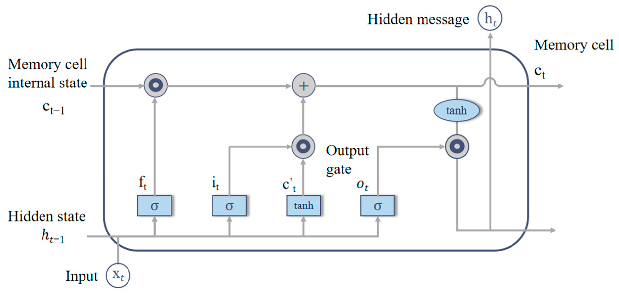
2.2. Long Short-Term Memory Networks

LSTM was proposed by Hochreiter and Schmidhuber in 1997, and it is a variant of RNN network [33]. RNN is widely employed in time series prediction due to its ability to capture time dependencies. Compared to RNN, LSTM mitigates the issue of “gradient vanishing” caused by backpropagation during model training and exhibits long-term dependency learning capabilities, making it more suitable for processing traffic flow data. The schematic diagram of an LSTM network is depicted in Figure 1.

The LSTM related mathematical model formulas are shown in Equations (11)–(16), where x_t denotes the input data at moment t of the layer; h_t denotes the hidden information entered by the layer at moment t; f_t is for forgetting the door; i_t denotes an input gate; o_t denotes an output gate; and c_t denotes a memory cell. W, U denote weights, b denotes offset, σ denotes Sigmoid activation function, and Tanh denotes Tanh activation function.

$$f_t=\sigma \left(W_f{x}_t+U_f{h}_{t-1}+b_f\right)$$

(11)

$$i_t=\sigma \left(W_i{x}_t+U_i{h}_{t-1}+b_i\right)$$

(12)

$$c_t^{\prime }=\mathit{Tanh}\left(W_c{x}_t+U_c{h}_{t-1}\right)$$

(13)

$$c_t=f_t{c}_{t-1}+i_t{c}_t^{\prime }$$

(14)

$$h_t=o_t\mathit{Tanh}\left(c_t\right)$$

(15)

$$o_t=\sigma \left(W_o{x}_t+U_o{h}_{t-1}+b_o\right)$$

(16)

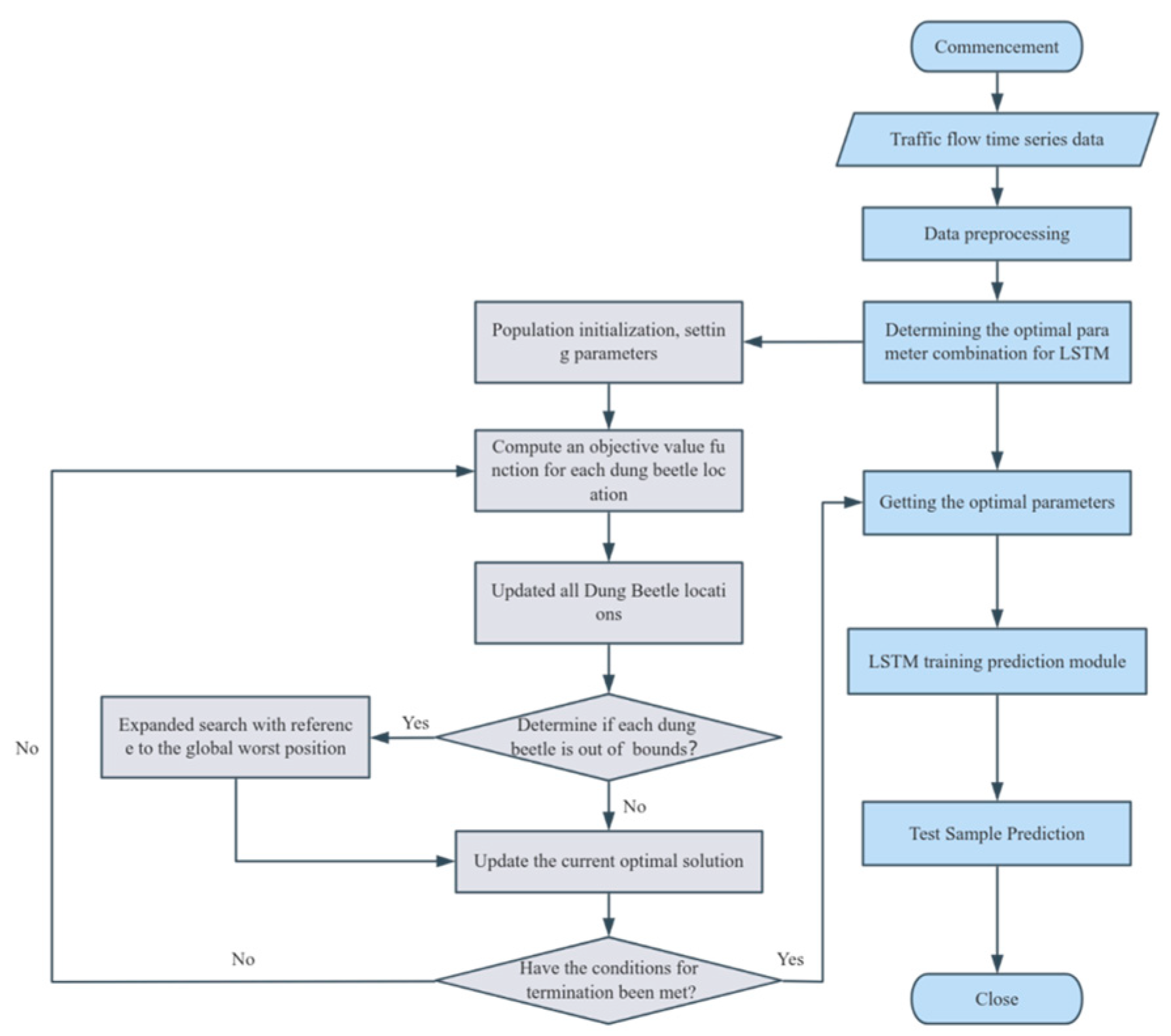
2.3. Combinatorial Predictive Modeling

In this paper, LSTM is used to feature-mine the historical data of traffic flow, and the parameters of vessel traffic flow, traffic flow speed, and traffic flow density are extracted from the AIS data as inputs to the LSTM model, which in turn predicts the future traffic flow data in the watershed. The performance of the LSTM model is highly dependent on the setting of several parameters, including the number of layers, the number of neurons per layer, the batch size, etc., and the selection of an appropriate combination of hyperparameters is crucial for the model. To address the model instability caused by hyperparameters in the LSTM network, this paper further introduces DBO to optimize and improve the look-back, the number of hidden units in the 1st layer network, the number of hidden units in the 2nd layer network, the number of hidden units in the 3rd layer network, the dropout, the batch size, and a total of 6 parameters of the LSTM network, and the DBO algorithm is finally found after many iterations. The combination of hyperparameters minimizes the prediction error of the LSTM model on the validation set, thus improving the prediction accuracy and generalization ability. The flow of the constructed DBO-LSTM ship traffic flow prediction model is shown in Figure 2.

The specific steps of the model are as follows:

• Data preprocessing. The historical traffic flow data are first divided into training set and test set, after which they are normalized separately.
• Initialize the population and parameters, and determine the number of nodes in each network layer.
• Model solving. Use the mean square error (MSE) of the LSTM prediction results as the fitness function to obtain the individual fitness of each dung beetle.
• Location update. Judge whether each dung beetle is within the boundary; if not, expand the search range with reference to the global worst position; if it is within the boundary, update the current optimal solution directly.
• Judge whether the termination condition is reached. If not, continue the iterative search for optimization, and if it is reached, terminate the algorithm and output the optimal parameter combination. LSTM is used for training and testing.

The following are the definitions of the relevant parameters in the DBO-LSTM model:

Look-back: it refers to the number of time steps to look forward at each time step while training the model. It defines the length of historical information of the model.

• Neurons1, Neurons2, Neurons3 (number of neurons): these parameters indicate the number of neurons in each hidden layer in the DBO-LSTM layer. Usually, the number of neurons in each hidden layer can be adjusted according to the complexity of the task.
• Dropout (dropout rate): dropout is a regularization technique used to reduce overfitting of the model. It specifies the percentage of neurons that are randomly discarded during training.
• Batch size: batch size indicates the number of samples used in each update of the model during training. Larger batch sizes may improve training speed, but may increase memory requirements.
• Epochs: epochs refer to the number of complete traversals of the training dataset. Each epoch contains a series of forward-propagation and back-propagation for updating the weights of the model.
• Optimizer: an optimizer is an algorithm used to update the model weights to reduce the loss function. Common optimizers include Stochastic Gradient Descent (SGD), Adam, RMSprop, and so on.

2.4. Definition of Vessel Traffic Flow Parameters

Vessel traffic flow parameters are divided into macro-parameters and micro-parameters. Macro-parameters are mainly used to describe the overall operation status of vessel traffic flow, which mainly includes the following: traffic flow, traffic flow speed, traffic flow density, traffic flow direction, etc. Micro-parameters are mainly used to describe the movement characteristics of vessels related to each other in the traffic flow. In this paper, according to the actual situation of the waters, we choose to predict the traffic flow, traffic density, and traffic speed.

Water traffic is different from the one-dimensional movement of vehicles in road traffic; the movement of ships is two-dimensional, so the relevant macroscopic parameters of vessel traffic flow are as follows: traffic flow, traffic flow density, traffic flow speed, traffic flow width, and traffic flow direction. Vessel traffic flow prediction is usually the prediction of the macro-parameters of traffic flow; this paper is based on the actual situation of the waters, the traffic flow, traffic flow density, and traffic flow speed prediction study.

• Vessel traffic flow

Vessel traffic flow size can reflect the scale of traffic in the waters and the degree of busy-ness, but also to a certain extent to reflect the degree of traffic congestion in the waters and the degree of danger. The formula is shown in Equation (17).

$$Q=\frac{N}{T}$$

(17)

In the above equation, Q denotes the average number of traffic flows through the waters in a unit of time; N denotes the number of all vessels in the waters in a given time period, in units of vessel trips; and T denotes the length of time of the observation.

• Vessel traffic speed

Vessel traffic flow speed refers to the distance passed by the vessel in unit time, which can be used to evaluate the degree of smoothness of the waters, due to the different references of the selected area and the different focus points of the study; the vessel speed is divided into the speed of the ground, the time-averaged speed, and the interval-averaged speed. In this paper, we mainly consider the time-averaged speed, which refers to the average value of the speed of all the ships passing through a certain cross-section of the water or a certain node, and its formula is shown in Equation (18).

$$V=\frac{{\displaystyle \sum _{i=1}^N}{v}_i}{N}$$

(18)

In the above equation, V denotes the time-averaged speed in knots; N denotes the number of all ships in the waters in a given time period in units of ships; and vi denotes the instantaneous speed in knots of the ith ship passing through a certain cross-section of water or a certain node in relation to the ground.

• Vessel traffic density

Vessel traffic flow density refers to the number of vessels in a unit area of water at a certain instant, the size of which on the one hand can reflect the dense degree of vessels in the waters, and on the other hand can reflect to a certain extent the degree of traffic congestion and the degree of danger in the waters. Its specific formula is shown in Equation (19).

$$\rho =\frac{N}{S}$$

(19)

In the above equation, ρ denotes the density of vessel traffic flow in vessels/square nautical miles; N denotes the number of all vessels in the waters at a given time period in vessels; and S denotes the area of the waters in square nautical miles.

3. Results

3.1. Data Sources and Data Processing

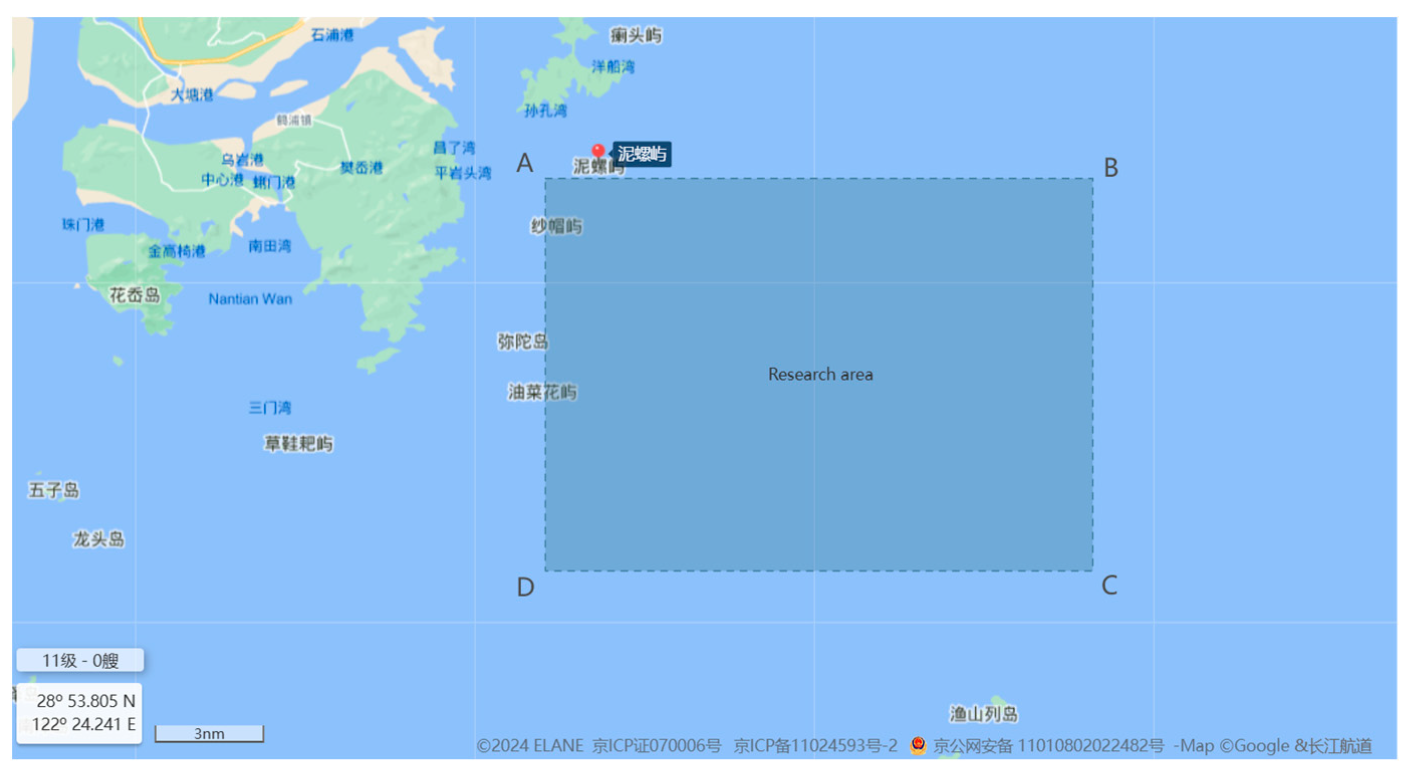
3.1.1. Data Sources

In this paper, the data are adopted from the AIS data of Xiangshan Port of Ningbo Maritime Bureau from 1 February 2023 to 29 April 2023, and the delineated study area is a rectangle with the latitude and longitude of its four vertices as A (122.0246° E, 29.1253° N), B (122.3079° E, 29.1253° N), C (122.3079° E. 28.9481° N), D (122.0246° E, 28.9481° N), and the region is shown in Figure 3.

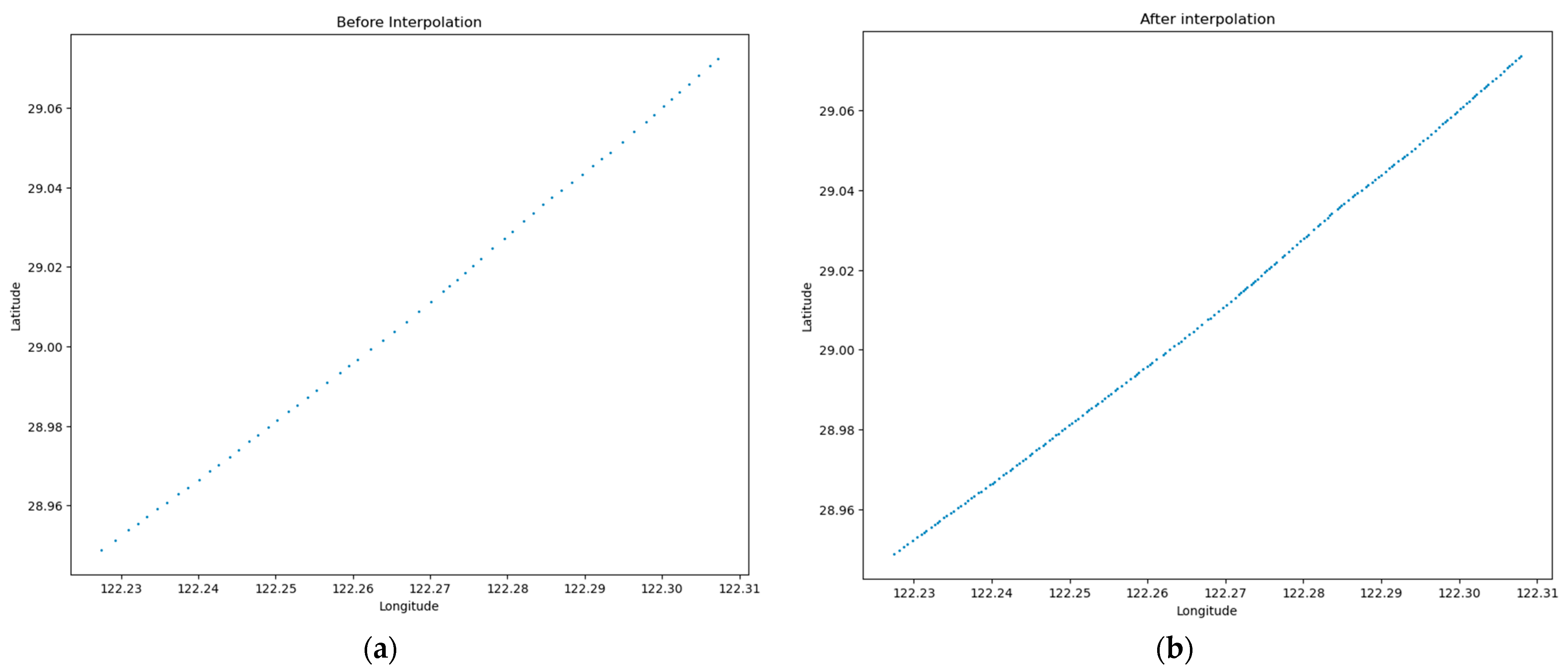
3.1.2. Data Processing

The original AIS data are subject to environmental disturbances and their own stability factors during the operation of the relevant equipment, which leads to the problem of duplicate, missing, or abnormal data, and the common abnormal data include abnormal position (e.g., crossing the land, etc.), mismatch of latitude, longitude, and speed (e.g., latitude and longitude change but speed is 0), unstable speed (e.g., sudden change in speed data and the time interval of the sudden change point is very short), and so on. These errors cannot reflect the real state of vessel traffic flow, which affects the calculation of relevant parameters of traffic flow. These erroneous AIS data cannot reflect the real state of vessel traffic flow, thus affecting the calculation of traffic-flow-related parameters, so it is necessary to process the original AIS data with appropriate methods.

In this paper, the duplicate and abnormal data are deleted from the operation and made up as missing values. In this paper, the Lagrange interpolation method is used for its complementary operation; the Lagrange interpolation method is applied in numerical analysis, and its basic principle is as follows: if the function value y₀, y₁, ..., y_n is known to be y = f(x) at mutually different n + 1 points x₀, x₁, ..., x_n, then a function p(x) can be constructed that passes through these n + 1 points no more than n times, as shown in Equation (20) below. More than n functions of p(x)) are shown in Equation (20) below.

$$p\left(x_k\right)=y_k,k=0,1,\mathrm{\dots },n$$

(20)

Then p(x) is said to be the interpolating function of f(x) at the point x_k. p(x) is a function close to the unknown original function f(x), so the value of the interpolating function p(x) can be taken as an approximation of the exact value f(x) at any point, and the expressions of the Lagrange interpolating polynomials are shown in the following Equations (21) and (22).

$$L_n\left(x\right)={\displaystyle \sum _{k=0}^{n-1}{y}_k{p}_k\left(x\right)}$$

(21)

$$p_k\left(x\right)={\displaystyle {\prod }_{j=0,j\ne k\frac{x-x_j}{x_k-x_j}}^n}$$

(22)

The changes before and after the abnormal interpolation operation of ship data are as follows, as shown in Figure 4. From the figure, it can be seen that the trajectory curve after processing is smoother and conforms to the motion curve of the ship under normal sailing condition.

3.2. Extraction of Vessel Traffic Flow Parameters

3.2.1. Vessel Traffic Flow Extraction Method

Firstly, the intercepted AIS data in the water area are statistically grouped according to 1 h, and then according to the MMSI number of each vessel, the vessels in a single time interval are de-weighted, i.e., each vessel is only counted once in this time interval, and then the total number of data samples in each time interval can be calculated to obtain the corresponding time period of the vessel traffic flow.

3.2.2. Vessel Traffic Speed Extraction Method

With waterborne traffic, compared with road traffic, it is difficult to effectively calculate the interval average speed within a segment or within a water area. For a specific ship in the study waters, to find its sampling time interval, the speed of all trajectory points for the arithmetic average must be found; and then the study of all the average speeds of the ship in the waters of the average value of the speed of the ship is sought to perform another arithmetic average, after which you can obtain the waters of a specific time interval of the speed of the traffic flow.

3.2.3. Vessel Traffic Density Extraction Method

According to the definition of vessel traffic flow density, it can be seen that it is an instantaneous value for a certain water area interval, which changes with time and space. The vessel traffic flow parameters studied in this paper are for a certain time interval, and the frequency of AIS data transmission of each vessel is not the same, so it is difficult to measure the vessel traffic flow density in the actual situation, taking into account that there is a great correlation between the vessel traffic flow and the vessel traffic flow density; therefore, in this section, the vessel traffic flow and the area of the research waters are used to carry out a certain amount of calculations to obtain the alternative value of the vessel traffic flow density. In this section, the traffic flow and the area of the research waters are calculated to obtain the alternative value of the vessel traffic flow density. The calculation method is as follows: first, all the data are statistically grouped according to 1 h time intervals, then the data are statistically grouped according to 0.5 h for each 1 h time interval, and then the ratio of vessel traffic flow to the area of the study waters is calculated for each 0.5 h time interval, and finally the arithmetic mean is taken as the density of vessel traffic flow within the study waters for each 1 h time interval in the statistical sense.

3.3. Dataset

The short-term prediction of vessel traffic flow for the time interval is not clearly divided into standards, compared with road transport, because the change frequency of water transport is not as high as that of road transport, and, at the same time, reference to the short-term prediction of road transport intervals is not more than 15 min. This paper selects the time interval of 1 h to build the vessel traffic flow dataset, with the density of traffic flow and the traffic flow speed dataset formed to remain the same with the experimental setup of the training set and test set data for 9:1. The experimental setup of the training set and test set data is 9:1. The parameter data are experimental, and some of the vessel traffic flow datasets are shown in

Table 1. Partial vessel traffic flow dataset.

Data Sequence Number	Time Period (Hour)	Vessel Traffic Flow (Vessels)	Vessel Traffic Flow Speed (kn)	Vessel Traffic Flow Density (Vessels/Square Nautical Mile)
1	2023/2/1 0:00	88	3.63	27.56
2	2023/2/1 1:00	70	2.37	22.47
…	…	…	…	…
2110	2023/4/29 21:00	95	7.20	25.98
2111	2023/4/29 22:00	148	7.71	38.10
2112	2023/4/29 23:00	143	8.22	39.15

.

Different evaluation indicators have different magnitudes when assessing the prediction effect, but they will affect the results of the data analysis; in order to eliminate the effect of the magnitude between the indicators, before conducting the prediction experiment, the historical data will be normalized by 0–1, and then the data will be inverse normalized after obtaining the prediction results, and the corresponding error will be calculated. In this paper, Min–Max normalization is selected, as shown in Equation (23).

$$W_i^{\prime }=\frac{W_i-\min \left(W_i\right)}{\max \left(W_i\right)-\min \left(W_i\right)}$$

(23)

In the above equation, w_i^’ denotes the normalized traffic flow data; w_i denotes the ith traffic flow data; max (w_i) and min (w_i) denote the maximum and minimum values, respectively.

3.4. Experimental Results

3.4.1. Analysis of the Superiority of the DBO Algorithm

In order to verify the superiority of DBO, this paper selects 12 test functions in CEC2017 [34] to compare and analyze PSO, grey wolf optimizer (GWO), SSA, whale optimization algorithm (WOA), and DBO. Among them, F1 and F3 are selected for single peak function; F4, F7, and F8 are selected for simple multi-peak function; F13, F15, and F19 are selected for hybrid function; and F22, F23, F26, and F28 are selected for combinatorial function. The formulas of the above 12 benchmark test functions are shown in

Table 2. Test function formulas.

Function Categories	Test Functions	Dimension	Range of Independent Variables	Theoretical Value
Unimodal functions	CEC1	30	[−100, 100] D *	100
	CEC3	30	[−100, 100] D	300
Simple multimodal functions	CEC4	30	[−100, 100] D	400
	CEC7	30	[−100, 100] D	700
	CEC8	30	[−100, 100] D	800
Hybrid functions	CEC13	30	[−100, 100] D	1300
	CEC15	30	[−100, 100] D	1500
	CEC19	30	[−100, 100] D	1900
Composition functions	CEC22	30	[−100, 100] D	2200
	CEC23	30	[−100, 100] D	2300
	CEC26	30	[−100, 100] D	2600
	CEC28	30	[−100, 100] D	2800

* D: dimensions.

.

The number of PSO, GWO, SSA, WOA, and DBO iterations selected for the algorithm comparison experiments is 500, and the experimental tool is MATLAB R2022a, some of whose parameters are shown in

Table 3. Some parameters of the algorithm.

Algorithm	Parameter	Value
DBO	k	0.1
	b	0.3
	s	0.5
PSO	Topology	Fully connected
	C1	2
	C2	2
GWO	amin	0
	amax	2
SSA	Leader position update	0.5
	probability
	V0	0
WOA	ɑ	Decreased from 2 to 0

.

The superiority comparison experiments conducted by the above five algorithms to solve each test function are shown in Figure 5, and the results of the experiments are shown in

Table 4. Algorithm comparison experiment results.

		DBO	PSO	GWO	SSA	WOA
F1	BEST	290.54	3,043,455.62	996,495,230.04	66,043.62	2,536,752,041.83
	STD	5787.82	176,277,337.26	2,017,790,760.95	1,560,777,518.97	1,231,407,961.33
	AVG	5456.92	248,649,968.86	3,313,768,370.92	964,564,053.40	4,756,114,730.11
F3	BEST	27,086.66	64,647.93	33,642.33	65,366.26	149,361.16
	STD	10,275.73	34,239.17	21,283.26	36,665.42	60,711.10
	AVG	46,632.03	95,141.18	63,377.32	97,545.74	259,184.93
F4	BEST	404.17	516.14	523.10	468.21	747.69
	STD	28.06	204.55	58.99	228.63	403.88
	AVG	500.26	693.62	609.15	658.88	1472.44
F7	BEST	830.34	921.94	836.11	1144.54	862.84
	STD	35.60	89.06	53.35	70.30	115.69
	AVG	882.03	1116.49	917.14	1313.88	1015.86
F8	BEST	861.57	980.18	865.19	905.52	928.82
	STD	29.31	54.19	23.82	58.78	26.04
	AVG	905.53	1069.17	905.88	1019.02	980.14
F13	BEST	2033.01	5897.09	31,976.54	81,077.38	878,582.42
	STD	1,349,367.13	23,844.93	20,342,174.55	56,807,033.72	50,058,920.84
	AVG	477,203.45	31,761.84	12,491,682.16	17,643,672.55	19,316,335.79
F15	BEST	1752.17	1840.76	5603.07	1876.29	201,676.74
	STD	11,235.37	8581.38	1,323,884.66	8576.14	8,061,592.55
	AVG	12,031.02	8119.29	321,947.60	8177.42	7,399,521.03
F19	BEST	1972.78	2097.15	14,414.23	8948.28	92,326.72
	STD	381,128.99	9127.73	7,704,779.30	7,479,505.78	911,157.77
	AVG	88,850.83	9019.18	3,464,630.50	2,961,040.96	2,633,039.41
F22	BEST	2300.02	2370.01	2311.10	2471.88	2950.73
	STD	2129.34	2576.807	2061.98	2110.97	1914.14
	AVG	5678.16	4902.998	4330.72	5425.15	8033.52
F23	BEST	2716.51	2755.37	2867.65	2745.08	2944.67
	STD	64.50	90.95	103.40	79.42	101.98
	AVG	2807.46	2904.32	3023.63	2919.58	3146.57
F26	BEST	2800.15	4341.23	2817.11	4024.52	4949.68
	STD	1132.02	421.55	1120.76	995.52	1226.52
	AVG	6428.55	5081.44	5052.05	6996.78	8314.16
F28	BEST	3193.02	3218.89	3306.92	3279.85	3506.11
	STD	18.17	115.43	104.87	774.83	273.09
	AVG	3221.97	3323.06	3479.73	3694.62	3820.83

below, where the bold numbers are the best results. Compared with other algorithms, DBO has a significantly superior convergence speed in solving the single peak function F1, and its convergence speed is also better than PSO, GWO, SSA, and WOA in the late stage of solving F3, although it is not so significant in the early stage of solving F1. Combined with Table 4, the optimal value, standard deviation, and average value of DBO in solving the single-peak function are all optimal; in solving the simple multi-peak functions F4, F7, and F8, the convergence speed of DBO is faster, and the best results are shown in bold numbers. When solving the simple multi-peak functions F4, F7, and F8, DBO converges faster, although it is not significantly superior in solving the late stage of F4. Combined with the analysis in Table 4, it can be seen that DBO achieves the best in terms of optimal value, standard deviation, and mean, and there is not much difference with the optimal GWO in terms of standard deviation when solving F8; when solving the mixed functions F13, F15, and F19, DBO is able to effectively avoid the local optimum and eventually converges to the optimal position in the search space, as seen in Table 4. From Table 4, DBO achieves the best in terms of optimal values, and is only second to PSO in terms of standard deviation and mean value; when solving the combined functions F22, F23, F26, and F28, DBO also converges quickly in the early iteration period, and the analysis of Table 4 shows that DBO achieves the best in terms of optimal values. Comparative experimental results show that the proposed use of DBO has a higher success rate than the current state-of-the-art optimization algorithms, with better applicability and effectiveness.

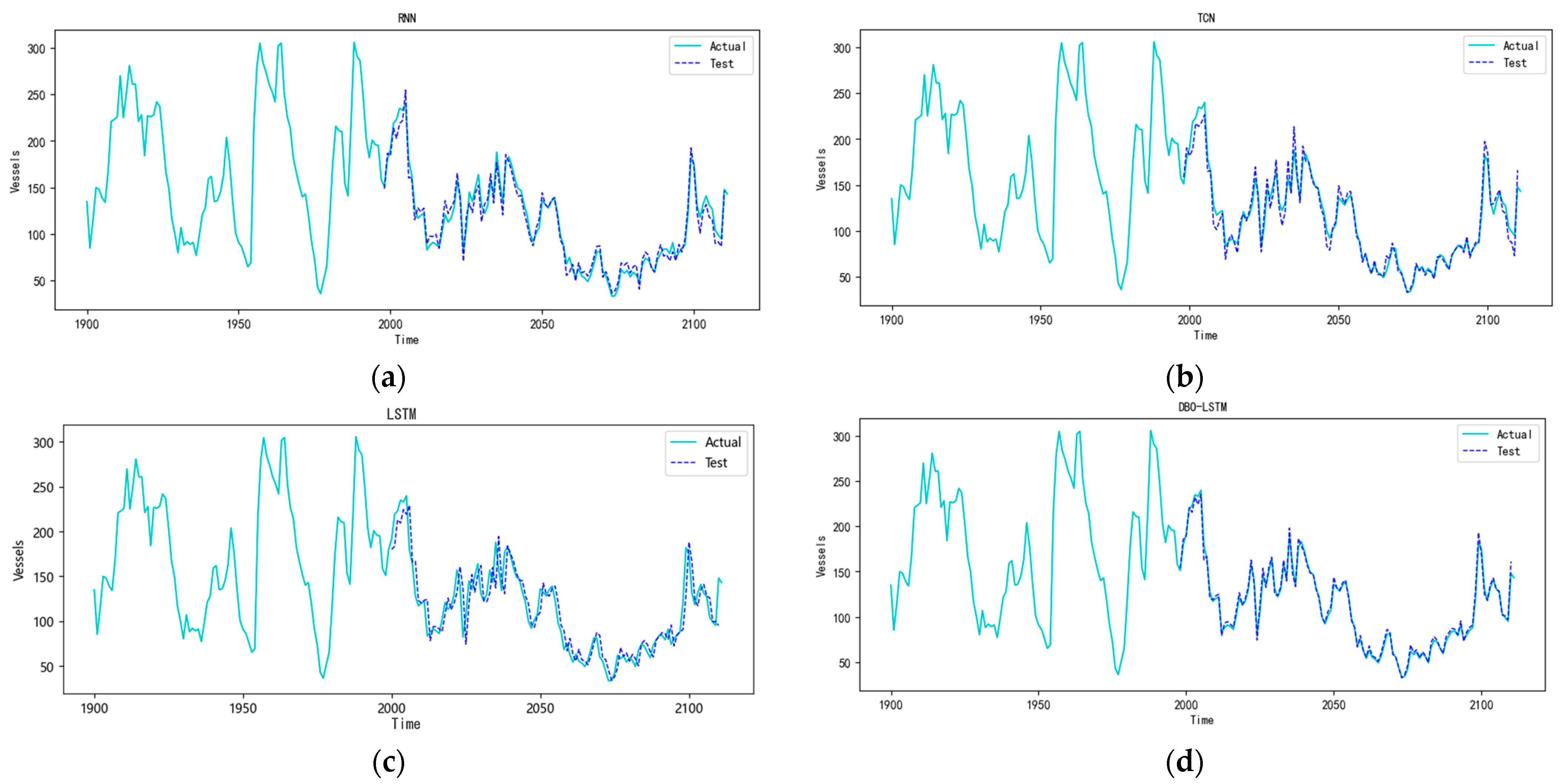
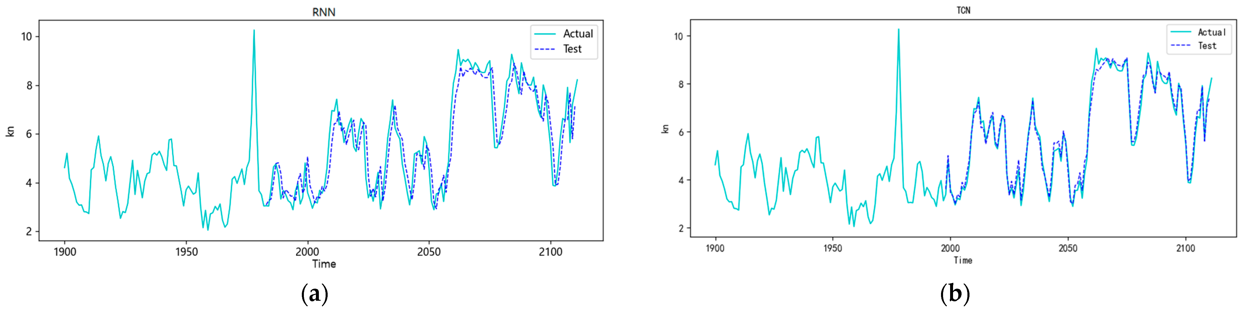
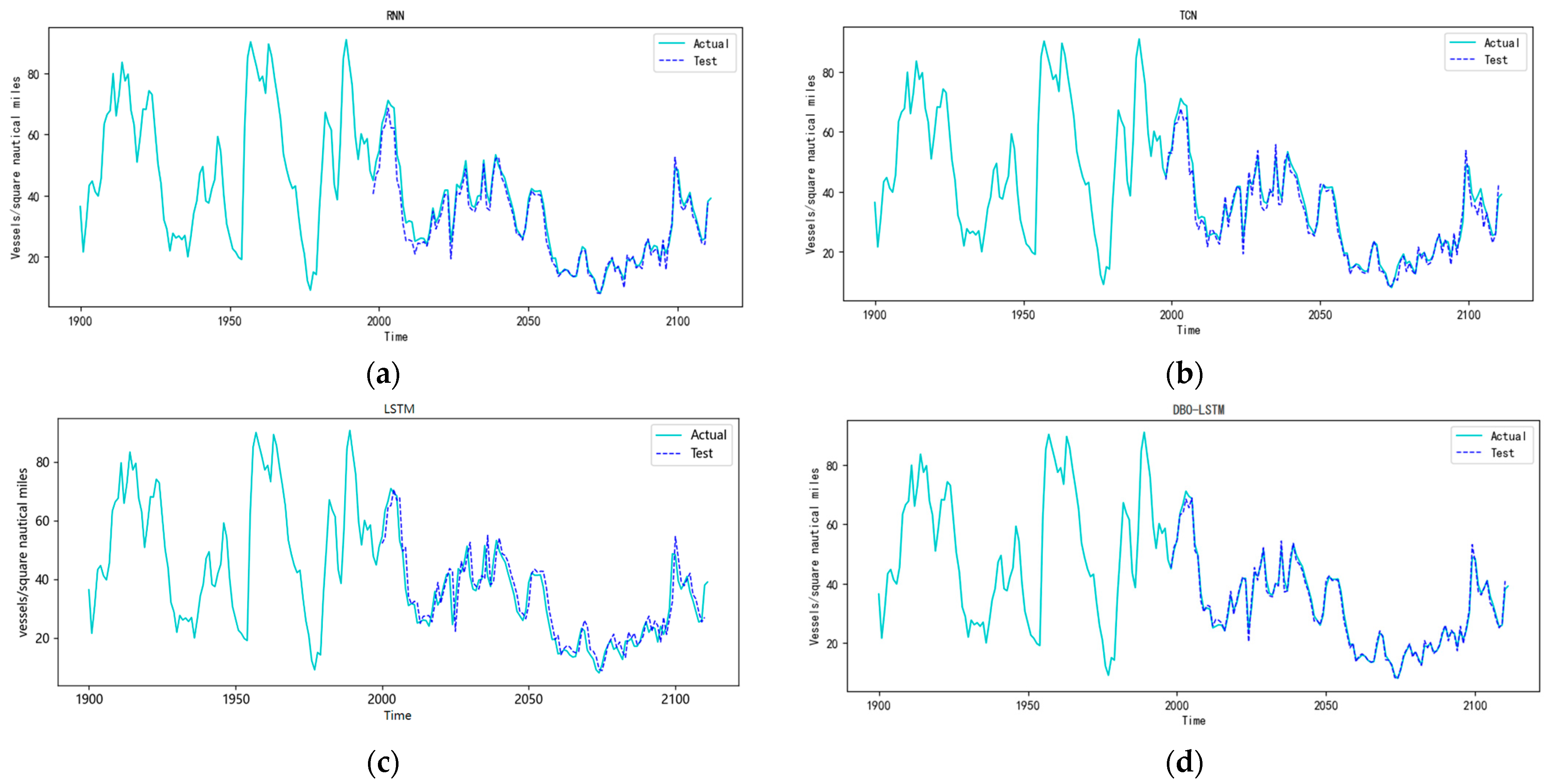
3.4.2. Analysis of DBO-LSTM Model Prediction Effect

In order to illustrate the prediction accuracy of the DBO-LSTM model more clearly, this paper introduces three error evaluation indexes, namely, mean absolute error (MAE), root mean square error (RMSE), and mean relative error (MRE), which are convenient for objectively evaluating the prediction effect of the prediction model. Their calculation formulas are shown in Equations (24)–(26), respectively.

$$MAE=\frac{1}{N}{\displaystyle \sum _{k=1}^N\left|x_k-x_k^{\prime }\right|}$$

(24)

$$RMSE=\frac{1}{N}\sqrt{{{\displaystyle \sum _{k=1}^N\left(x_k-x_k^{\prime }\right)}}^2}$$

(25)

$$MRE=\frac{1}{N}{\displaystyle \sum _{k=1}^N\left|\frac{x_k-x_k^{\prime }}{x_k}\right|}$$

(26)

In the above equation, x_k is the true value, x_k’ is the predicted value, and N is the number of traffic flow data. The lower the evaluation index, the lower the proof of error, i.e., the model prediction accuracy is higher and the prediction ability is stronger.

In order to compare the prediction performance of the proposed DBO-LSTM model, a total of four models, including RNN, temporal convolutional network (TCN), LSTM base model, and DBO-LSTM, are used for comparison, and the number of the DBO population is set to be 30, and the number of iterations is set to be 10, and the DBO-LSTM model has the best parameter combinations, as shown in

Table 5. Optimal parameter combinations for the DBO-LSTM model.

DBO-LSTM Model Parameter Values	Prediction Model for Each Traffic Flow Parameter
	Vessel Traffic Flow	Vessel Traffic Flow Speed	Vessel Traffic Flow Density
look-back	100	81.7142	100
nenurous1	128	42.1858	64.3353
nenurous2	125.8540	74.6762	128
nenurous3	84.7515	17.0829	111.6725
dropout	0.4155	0.0846	0.5
batch size	40.0226	19.7517	62.6214
epochs	100	100	100
optimizer	Adam	Adam	Adam

. The MAE, RMSE, and MRE error metrics of each model for predicting the three traffic flow parameters are shown in

Table 6. Comparison of prediction error metrics.

Model	Vessel Traffic Flow			Vessel Traffic Flow Speed			Vessel Traffic Flow Density
	MAE	RMSE	MRE	MAE	RMSE	MRE	MAE	RMSE	MRE
RNN	17.14	1.78	0.13	0.61	0.06	0.14	5.29	0.52	0.15
TCN	18.89	1.77	0.68	0.60	0.06	0.45	5.69	0.53	0.83
LSTM	12.99	1.70	0.13	0.60	0.05	0.13	5.12	0.51	0.14
DBO—LSTM	8.70	1.09	0.05	0.32	0.02	0.08	1.43	0.37	0.05

.

From Table 6, it can be seen that the MAE, RMSE, and MRE error values of DBO-LSTM are the smallest in predicting the three traffic flow parameters, and the accuracy of predicting each traffic flow parameter is the highest, which is 95%, 92%, and 95%, respectively. Compared with the RNN model, the DBO-LSTM model reduces the three errors of MAE, RMSE, and MRE by 49.2%, 38.8%, and 61.5%, respectively, when predicting traffic flow; it reduces the three errors of MAE, RMSE, and MRE by 47.5%, 66.7%, and 42.9%, respectively, when predicting traffic speed; and the three errors of MAE, RMSE, and MRE when predicting traffic density were reduced by 73.0%, 28.8%, and 66.7%, respectively. Compared with the TCN model, the DBO-LSTM model reduces the MAE, RMSE, and MRE3 errors by 53.9%, 38.4%, and 92.6% when predicting the traffic flow; by 46.7%, 66.7%, and 82.2% when predicting the traffic flow speed; and the MAE, RMSE, and MRE3 errors when predicting the traffic flow density were reduced by 74.9%, 30.2%, and 94.0%, respectively. Compared with the LSTM model, the DBO-LSTM model reduces the MAE, RMSE and MRE3 errors by 33.0%, 35.9%, and 61.5%, respectively, when predicting traffic flow; it reduces the MAE, RMSE, and MRE3 errors by 46.7%, 60.0%, and 38.5%, respectively, when predicting traffic flow speed; and it reduces the MAE, RMSE, and MRE3 errors when predicting traffic flow density by 72.1%, 27.5%, and 64.3%, respectively. This shows that the DBO-LSTM model can realize more accurate traffic flow prediction than the basic model, and has better generalization.

The results of the proposed DBO-LSTM model for predicting each traffic flow parameter are visualized as shown in Figure 6, Figure 7 and Figure 8. From the figure, it can be seen that the DBO-LSTM model can reflect the volatility of the data well, and its prediction fits the real value to a high degree, which can reflect the change in vessel traffic flow more realistically.

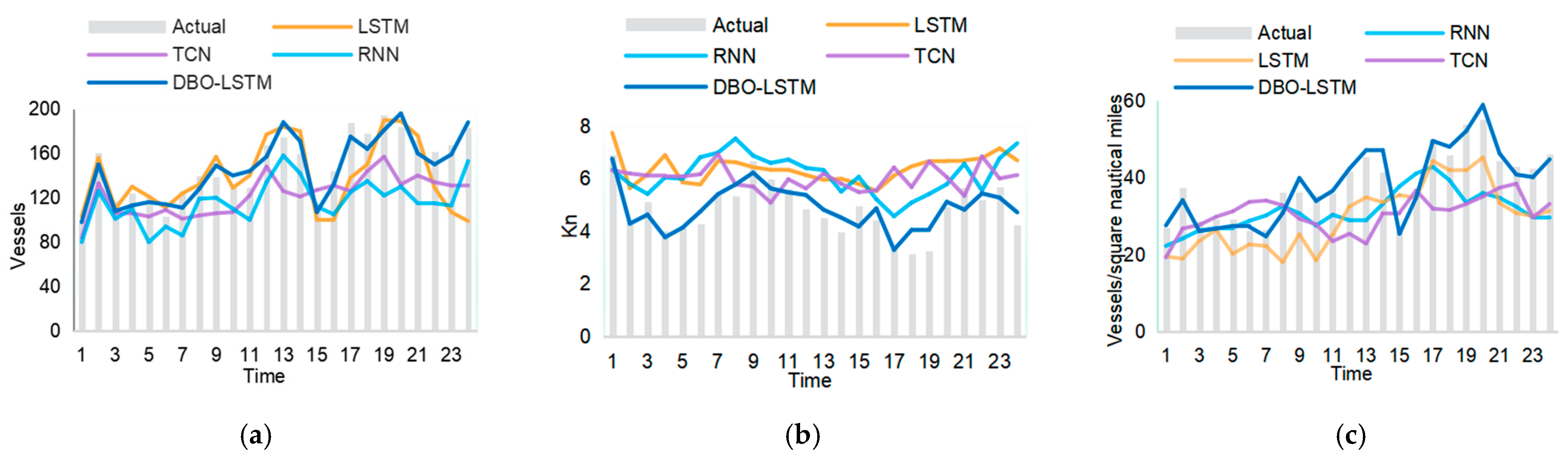
3.4.3. Future Vessel Traffic Flow Prediction Based on DBO-LSTM

Using RNN, TCN, LSTM, and DBO-LSTM to predict the traffic flow within the next 24 h (i.e., from 00:00 30 April 2023 to 23:00 30 April 2023) in some of the waters of the coastal port area of Monsanto, respectively, and then calculating the error with the real data on 30 April 2023, the error indexes of the prediction of each model for the three types of traffic flow parameters in the next 24 h in the study waters are shown in

Table 7. Comparison of the error indexes of traffic flow parameters predicted by each model in the next 24 h.

Model	Vessel Traffic Flow			Vessel Traffic Flow Speed			Vessel Traffic Flow Density
	MAE	RMSE	MRE	MAE	RMSE	MRE	MAE	RMSE	MRE
RNN	49.38	11.18	0.33	2.10	0.49	0.48	10.72	2.55	0.27
TCN	22.88	5.47	0.15	1.24	0.30	0.29	8.73	2.23	0.21
LSTM	18.17	5.68	0.12	1.78	0.41	0.42	17.18	3.88	0.42
DBO-LSTM	10.75	2.26	0.07	0.40	0.10	0.09	2.16	0.52	0.06

.

As can be seen from Table 7, DBO-LSTM also achieves better results in predicting future traffic flow experiments, with minimum values of MAE, RMSE, and MRE compared to the three base models. It can be concluded that the DBO-LSTM model has some generalization ability. The values of each traffic flow parameter predicted by the three base models and the DBO-LSTM model for the next 24 h are visualized in comparison with the real data, and the results are shown in Figure 9.

In the above figure, the dark blue folded line represents the traffic flow prediction result of the DBO-LSTM model for the next 24 h, and the light blue bar graph represents the real value of the dataset, and this figure visualizes the comparison between the predicted value and the real value of each model, which shows that the DBO-LSTM model has a good performance in capturing the trend. In addition, through Table 6 above, it is found that under the prediction of different traffic flow parameters, the error is maintained within a reasonable range, and the accuracy of predicting the three parameters reaches 93%, 91%, and 94%, respectively, with better stability compared to the comparison model, which indicates that the model performs well in dealing with uncertainty, and it is shown through Table 6 and Figure 8 that the DBO-LSTM model performs well in trend prediction and can provide reliable prediction results.

4. Conclusions

Vessel traffic flow has strong nonlinear and complexity characteristics; in order to improve the accuracy of vessel traffic flow prediction, this paper proposes a DBO-LSTM vessel traffic flow prediction model. The DBO algorithm is used to iteratively optimize the hyperparameter combinations of LSTM, and experiments are conducted through the constructed prediction models of vessel traffic flow, vessel traffic flow speed, and vessel traffic flow density, respectively. Combined with the actual situation of the waters and the practical significance of traffic flow prediction, the scope of traffic flow prediction is determined to be the prediction of short-term vessel traffic flow within 24 h, and the dataset is divided into groups of every 1 h, and the prediction is carried out by the traffic flow data of a part of the waters in the coastal port area of Xiangshan, which is compared with the prediction models of RNN, TCN and LSTM. The results show that the proposed DBO-LSTM vessel traffic flow prediction model has a prediction accuracy of 95%, 93%, and 95% for the three parameters, respectively, and then predicts the three parameters in the next 24 h in this water area with an accuracy of 93%, 91%, and 94%, respectively, which indicates that it has a better prediction accuracy compared with the RNN, TCN, and LSTM prediction models, and can accurately predict the future traffic flow, which has certain effectiveness and feasibility. The ship traffic flow prediction method studied in this paper achieves ideal and accurate results, provides a certain theoretical basis for the research of risk assessment and navigation safety management of port waterways, assists the relevant maritime management departments to make reasonable decisions, reduces the pressure of navigation in the waters, and improves the efficiency of ship passage to a certain extent.

References

1. Cai, L.; Zhang, Z.; Yang, J.; Yu, Y.; Zhou, T.; Qin, J. A noise-immune Kalman filter for short-term traffic flow forecasting. Phys. A Stat. Mech. Its Appl. 2019, 536, 122601. [Google Scholar] [CrossRef]
2. He, W.; Zhong, C.; Sotelo, M.A.; Chu, X.; Liu, X.; Li, Z. Short-term vessel traffic flow forecasting by using an improved Kalman model. Clust. Comput. 2019, 22, 7907–7916. [Google Scholar] [CrossRef]
3. Xiao, X.; Duan, H. A new grey model for traffic flow mechanics. Eng. Appl. Artif. Intell. 2020, 88, 103350. [Google Scholar] [CrossRef]
4. Ahn, J.; Ko, E.; Kim, E.Y. Highway traffic flow prediction using support vector regression and Bayesian classifier. In Proceedings of the 2016 International Conference on Big Data and Smart Computing (BigComp), Hong Kong, China, 18–20 January 2016; pp. 239–244. [Google Scholar]
5. Williams, B.M. Modeling and Forecasting Vehicular Traffic Flow as a Seasonal Stochastic Time Series Process. Doctoral Dissertation, University of Virginia, Charlottesville, VA, USA, 1999. 9916358. [Google Scholar] [CrossRef]
6. Yin, H.; Wong, S.C.; Xu, J.; Wong, C. Urban traffic flow prediction using a fuzzy-neural approach. Transp. Res. Part C Emerg. Technol. 2002, 10, 85–98. [Google Scholar] [CrossRef]
7. Tian, X.; Zheng, Z.; Zeng, S. Research on the application of WLSM in Ship Traffic Fundamental Diagram Model. In Proceedings of the 2020 2nd International Conference on Robotics Systems and Vehicle Technology, Xiamen, China, 3–5 December 2020; pp. 39–44. [Google Scholar]
8. Zhao, S.; Wu, H.; Liu, C. Traffic flow prediction based on optimized hidden Markov model. J. Phys. Conf. Ser. 2019, 1168, 052001. [Google Scholar] [CrossRef]
9. Zhang, N.; Zhang, Y.; Lu, H. Seasonal autoregressive integrated moving average and support vector machine models: Prediction of short-term traffic flow on freeways. Transp. Res. Rec. 2011, 2215, 85–92. [Google Scholar] [CrossRef]
10. Liu, Y.; Wu, H. Prediction of road traffic congestion based on random forest. In Proceedings of the 2017 10th International Symposium on Computational Intelligence and Design (ISCID), Hangzhou, China, 9–10 December 2017; Volume 2, pp. 361–364. [Google Scholar]
11. Koochali, A.; Schichtel, P.; Ahmed, S.; Dengel, A. Probabilistic Forecasting of Sensory Data with Generative Adversarial Networks—ForGAN. IEEE Access 2019, 7, 63868–63880. [Google Scholar] [CrossRef]
12. Cai, L.; Lei, M.; Zhang, S.; Yu, Y.; Zhou, T.; Qin, J. A noise-immune LSTM network for short-term traffic flow forecasting. Chaos Interdiscip. J. Nonlinear Sci. 2020, 30, 023135. [Google Scholar] [CrossRef] [PubMed]
13. Zhao, L.; Wang, Q.; Jin, B.; Ye, C. Short-term traffic flow intensity prediction based on CHS-LSTM. Arab. J. Sci. Eng. 2020, 45, 10845–10857. [Google Scholar] [CrossRef]
14. Ma, D.; Song, X.; Li, P. Daily Traffic Flow Forecasting Through a Contextual Convolutional Recurrent Neural Network Modeling Inter-and Intra-Day Traffic Patterns. IEEE Trans. Intell. Transp. Syst. 2021, 11, 2627–2636. [Google Scholar] [CrossRef]
15. Fang, W.; Zhuo, W.; Song, Y.; Yan, J.; Zhou, T.; Qin, J. Δfree-LSTM: An error distribution free deep learning for short-term traffic flow forecasting. Neurocomputing 2023, 526, 180–190. [Google Scholar] [CrossRef]
16. Yu, W.; Du, T.; Zhang, W. Short-time traffic flow prediction using fuzzy wavelet neural network based on master-slave PSO. In Proceedings of the 2008 Fourth International Conference on Natural Computation, Jinan, China, 18–20 October 2008; Volume 3, pp. 321–325. [Google Scholar]
17. Luo, X.; Li, D.; Yang, Y.; Zhang, S. Short-term Traffic Flow Prediction Based on KNN-LSTM. J. Beijing Univ. Technol. 2018, 44, 1521–1527. [Google Scholar] [CrossRef]
18. Liu, F.; Wei, Z.; Huang, Z.; Lu, Y.; Hu, X.; Shi, L. A multi-grouped ls-svm method for short-term urban traffic flow prediction. In Proceedings of the 2019 IEEE Global Communications Conference (GLOBECOM), Waikoloa, HI, USA, 9–13 December 2019; pp. 1–6. [Google Scholar]
19. Qiao, Y.; Wang, Y.; Ma, C.; Yang, J. Short-term traffic flow prediction based on 1DCNN-LSTM neural network structure. Mod. Phys. Lett. B 2021, 35, 2150042. [Google Scholar] [CrossRef]
20. Zhou, W.; Wang, W. Multi-Step Short-Term Traffic Flow Prediction Based on a Novel Hybrid ARIMA-LSTM Neural Network. In Proceedings of the 20th COTA International Conference of Transportation Professionals, Xi’an, China, 14–16 August 2020. [Google Scholar] [CrossRef]
21. Zhang, K.; Chu, Z.; Xing, J.; Zhang, H.; Cheng, Q. Urban Traffic Flow Congestion Prediction Based on a Data-Driven Model. Mathematics 2023, 11, 4075. [Google Scholar] [CrossRef]
22. Zhang, Y.; Li, W. Dynamic maritime traffic pattern recognition with online cleaning, compression, partition, and clustering of AIS data. Sensors 2022, 22, 6307. [Google Scholar] [CrossRef] [PubMed]
23. Ismaeel, A.G.; Mary, J.; Chelliah, A.; Logeshwaran, J.; Mahmood, S.N.; Alani, S.; Shather, A.H. Enhancing Traffic Intelligence in Smart Cities Using Sustainable Deep Radial Function. Sustainability 2023, 15, 14441. [Google Scholar] [CrossRef]
24. Zhou, X.; Liu, Z.; Wang, F.; Xie, Y.; Zhang, X. Using deep learning to forecast maritime vessel flows. Sensors 2020, 20, 1761. [Google Scholar] [CrossRef] [PubMed]
25. El Mekkaoui, S.; Benabbou, L.; Caron, S.; Berrado, A. Deep Learning-Based Ship Speed Prediction for Intelligent Maritime Traffic Management. J. Mar. Sci. Eng. 2023, 11, 191. [Google Scholar] [CrossRef]
26. Su, G.; Liang, T.; Wang, M. Prediction of vessel traffic volume in ports based on improved fuzzy neural network. IEEE Access 2020, 8, 71199–71205. [Google Scholar] [CrossRef]
27. Xu, T.; Zhang, Q. Ship Traffic Flow Prediction in Wind Farms Water Area Based on Spatiotemporal Dependence. J. Mar. Sci. Eng. 2022, 10, 295. [Google Scholar] [CrossRef]
28. Hu, X.; Yan, Z.; Hao, Z. Predict Vessel Traffic with Weather Conditions Based on Multimodal Deep Learning. J. Mar. Sci. Eng. 2022, 11, 39. [Google Scholar] [CrossRef]
29. Li, Y.; Liang, M.; Li, H.; Yang, Z.; Du, L.; Chen, Z. Deep learning-powered vessel traffic flow prediction with spatial-temporal attributes and similarity grouping. Eng. Appl. Artif. Intell. 2023, 126, 107012. [Google Scholar] [CrossRef]
30. Zhang, Z.; Yin, J.; Wang, N.; Hui, Z. Vessel traffic flow analysis and prediction by an improved PSO-BP mechanism based on AIS data. Evol. Syst. 2019, 10, 397–407. [Google Scholar] [CrossRef]
31. Qing, L. Design of Online Monitoring System for Water Quality COD Based on Ultraviolet-Visible Spectroscopy. Master’s Thesis, Southwest University of Science and Technology, Mianyang, China, 2023. [Google Scholar]
32. Xue, J.; Shen, B. Dung beetle optimizer: A new meta-heuristic algorithm for global optimization. J. Supercomput. 2022, 79, 7305–7336. [Google Scholar] [CrossRef]
33. Hochreiter, S.; Schmidhuber, J. Long Short-Term Memory. Neural Comput. 1997, 9, 1735–1780. [Google Scholar] [CrossRef] [PubMed]
34. Awad, N.H.; Ali, M.Z.; Liang, J.J.; Qu, B.Y.; Suganthan, P.N. Problem Definitions and Evaluation Criteria for the CEC 2017 Special Session and Competition on Single Objective Bound Constrained Real-Parameter Numerical Optimization; Technical Report; Nanyang Technological University: Singapore, 2016; pp. 1–34. [Google Scholar]
Figure 1. LSTM network diagram.
Sustainability 16 05499 g001
Figure 2. DBO-LSTM predictive model flowchart.
Sustainability 16 05499 g002
Figure 3. Xiangshan coastal port research area: A–D are the four endpoints of the study area with latitude and longitude coordinates A (122.0246° E, 29.1253° N), B (122.3079° E, 29.1253° N), C (122.3079° E. 28.9481° N), and D (122.0246° E, 28.9481° N), respectively.
Sustainability 16 05499 g003
Figure 4. Lagrangian interpolation before and after treatment: (a) Lagrange interpolation before use; (b) Lagrange interpolation after use.
Sustainability 16 05499 g004
Figure 5. Comparison of convergence of various algorithms: (a) solve for the convergence of the F1 function; (b) solve for the convergence of the F3 function; (c) solve for the convergence of the F4 function; (d) solve for the convergence of the F7 function; (e) solve for the convergence of the F8 function; (f) solve for the convergence of the F13 function; (g) solve for the convergence of the F15 function; (h) solve for the convergence of the F19 function; (i) solve for the convergence of the F22 function; (j) solve for the convergence of the F23 function; (k) solve for the convergence of the F26 function; (l) solve for the convergence of the F28 function.
Sustainability 16 05499 g005
Figure 6. Prediction results of traffic flow: (a) demonstrating the RNN model to predict traffic flow; (b) demonstrating the TCN model to predict traffic flow; (c) demonstrating the LSTM model to predict traffic flow; (d) demonstrating the DBO-LSTM model to predict traffic flow.
Sustainability 16 05499 g006
Figure 7. Prediction results of traffic flow speed: (a) demonstrating the RNN model to predict traffic flow speed; (b) demonstrating the TCN model to predict traffic flow speed; (c) demonstrating the LSTM model to predict traffic flow speed; (d) demonstrating the DBO-LSTM model to predict traffic flow speed.
Sustainability 16 05499 g007aSustainability 16 05499 g007b
Figure 8. Prediction results of traffic flow density: (a) demonstrating the RNN model to predict traffic flow density; (b) demonstrating the TCN model to predict traffic flow density; (c) demonstrating the LSTM model to predict traffic flow density; (d) demonstrating the DBO-LSTM model to predict traffic flow density.
Sustainability 16 05499 g008
Figure 9. Prediction results of traffic flow parameters in the next 24 h: (a) comparison of flow parameter predictions; (b) comparison of speed parameter predictions; (c) comparison of density parameter predictions.
Sustainability 16 05499 g009