
Spatiotemporal Evolution of Green Finance and High-Quality Economic Development: Evidence from China


Abstract
:1. Introduction
2. Literature Review
2.1. Green Finance
2.2. High-Quality Economic Development
3. Research Methodology and Indicator Construction
3.1. Research Methodology
3.1.1. Entropy Weight Model
- Step 1. Normalization matrix:
- Step 2. The entropy value of the evaluation index is calculated to control the entropy value range to within (0,1). The formula for calculating the entropy value uses the natural logarithm and introduces a constant term. The formula is as follows:
- Step 3. The calculation of weights of evaluation indicators is as follows:
3.1.2. Coupling Coordination Model
3.1.3. Markov Chain
3.1.4. Mann-Kendall
3.2. Indicator Construction
3.2.1. Data Source and Preprocessing
3.2.2. Measurement of Green Finance Development
3.2.3. Measurement of High-Quality Economic Development
4. Results and Discussion
4.1. Green Finance Development Trend Analysis in China
4.1.1. Calculation of Green Finance Development Level
4.1.2. Analysis of the Changing Trend of Green Finance Development Level
- Regions with Significant Increasing Trends: Beijing, Tianjin, Shanghai, Zhejiang, Anhui, Jilin, Shandong, Hubei, Guangdong, Sichuan, and Shaanxi, among others, showed positive and significant MK test results, indicating a significant upward trend in green finance development during the study period. These regions likely benefited from strong policy support, financial product innovation, and increased investments in green initiatives, facilitating the growth of green finance.
- Regions with Significant Decreasing Trends: Inner Mongolia, Chongqing, Guizhou, Gansu, Qinghai, Ningxia, Xinjiang, and others exhibited negative and significant MK test results, suggesting a notable decline in green finance development over the study period. This trend could be attributed to insufficient investment in green finance, inadequate policy implementation, and weaker environmental protection awareness in these areas.
- Regions with No Significant Trends: Regions such as Hebei, Shanxi, Jiangsu, Hunan, Jiangxi, Guangxi, Yunnan showed no discernible upward or downward trends in green finance development based on the MK test results. This may indicate a stable development in green finance within these regions or insufficient influence from policies and market dynamics.
- Localized Variations: In certain areas like Fujian and Hainan, although overall trends were not significant, brief periods of both upward and downward trends were observed in specific years. These fluctuations could be linked to local policies, economic conditions, and environmental events, necessitating a further detailed analysis.
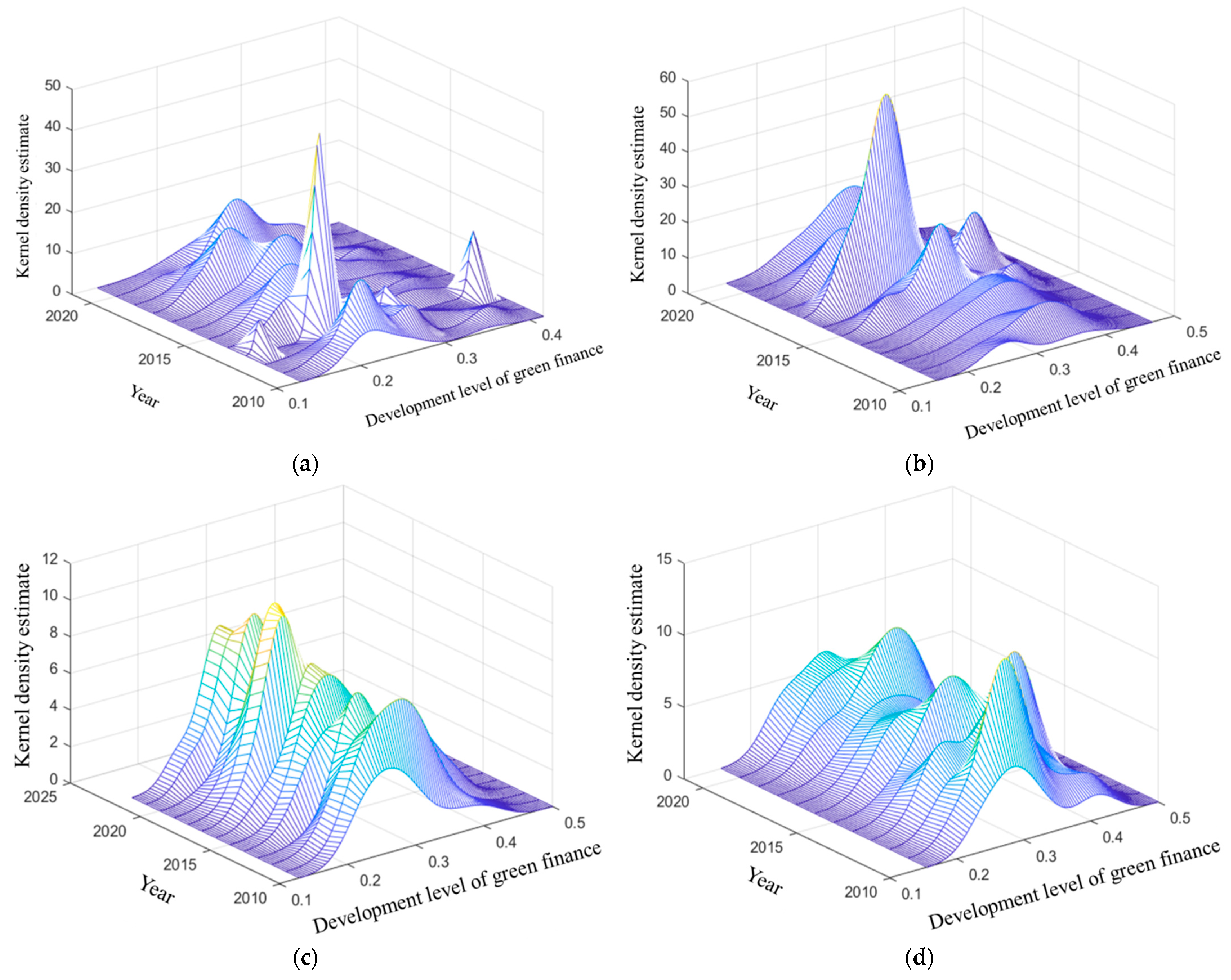
4.2. Spatial Evolution Analysis of Green Finance Development in China
4.3. Analysis of the Spatiotemporal Evolution Patterns of the Coupling Coordination between Green Finance and High-Quality Economic Development
4.3.1. Temporal Evolution Analysis of Coupling Coordination between Green Finance and High-Quality Economic Development
4.3.2. Spatial and Temporal Evolution Characteristics Analysis Based on Static (Spatial) Markov Model
- (1)
- All diagonal elements have values greater than those off the diagonal, with the maximum being 0.656 and the minimum being 0.409. This suggests that the probability of coupling coordination remaining unchanged is at least 40%, which is greater than the probability of a type transition. This indicates a constrained growth of coupling coordination between green finance and high-quality economic development, exhibiting “path dependence”.
- (2)
- Off-diagonal elements are situated on either side of the diagonal, indicating the potential for coupling coordination levels to transition to higher levels over consecutive years. However, such transitions are challenging, as most cities shift up or down by only one level. This is primarily due to the long-term and sustained nature of green finance and high-quality economic development. The advancement of green finance requires substantial time investment, coupled with factors such as geographical location and economic foundation, making significant type transitions unlikely over short periods.
- (3)
- The current stage of development is a transitional period between the level of green finance development and high-quality economic development. Regions are inclined to maintain their own type probabilities. In regions with high coupling coordination, there is a 24% probability of transitioning to a lower type, while regions with lower coupling coordination have around a 29% probability of transitioning to a higher type. This observation indicates a propensity for regression in regions exhibiting higher levels of coordination, underscoring the necessity of these regions to devise tailored development policies that address constraints on coordination development. It is crucial to promote comprehensive coordination between green finance and high-quality economic initiatives in local contexts.
5. Conclusions and Prospect
Author Contributions
Funding
Institutional Review Board Statement
Informed Consent Statement
Data Availability Statement
Conflicts of Interest
Appendix A. Calculation Results of Green Finance Maturity in All Provinces
| 2010 | 2011 | 2012 | 2013 | 2014 | 2015 | 2016 | 2017 | 2018 | 2019 | 2020 | 2021 | |
| Beijing | 0.0025 | 0.0021 | 0.0026 | 0.0028 | 0.0024 | 0.0029 | 0.003 | 0.0026 | 0.0026 | 0.0026 | 0.0026 | 0.0029 |
| Tianjin | 0.0028 | 0.0022 | 0.0023 | 0.002 | 0.002 | 0.0019 | 0.0013 | 0.0016 | 0.0021 | 0.0029 | 0.0019 | 0.002 |
| Hebei | 0.0029 | 0.0025 | 0.0025 | 0.0026 | 0.0025 | 0.0029 | 0.0025 | 0.0027 | 0.0027 | 0.0027 | 0.0028 | 0.0026 |
| Shanxi | 0.0043 | 0.0029 | 0.0029 | 0.0039 | 0.0037 | 0.004 | 0.0041 | 0.0036 | 0.0036 | 0.0041 | 0.0039 | 0.0032 |
| the Nei Monggol Autonomous Region | 0.0045 | 0.0044 | 0.0043 | 0.004 | 0.0042 | 0.0042 | 0.004 | 0.0045 | 0.0037 | 0.0035 | 0.0033 | 0.0038 |
| Liaoning | 0.0037 | 0.0026 | 0.0028 | 0.0023 | 0.0034 | 0.003 | 0.0024 | 0.0026 | 0.0026 | 0.0027 | 0.0026 | 0.0028 |
| Jilin | 0.0021 | 0.0022 | 0.0022 | 0.0022 | 0.0024 | 0.0022 | 0.0022 | 0.0022 | 0.0023 | 0.002 | 0.0019 | 0.0015 |
| Heilongjiang | 0.003 | 0.0024 | 0.0025 | 0.0032 | 0.0025 | 0.0024 | 0.0026 | 0.0028 | 0.0026 | 0.0034 | 0.0026 | 0.0022 |
| Shanghai | 0.0019 | 0.0014 | 0.0019 | 0.0014 | 0.0013 | 0.0012 | 0.0012 | 0.0013 | 0.0014 | 0.0018 | 0.0017 | 0.0019 |
| Jiangsu | 0.0024 | 0.0022 | 0.0023 | 0.0024 | 0.0021 | 0.0021 | 0.0021 | 0.002 | 0.0022 | 0.0019 | 0.0019 | 0.002 |
| Zhejiang | 0.0018 | 0.0017 | 0.0015 | 0.0017 | 0.0015 | 0.0017 | 0.0019 | 0.0018 | 0.0018 | 0.0022 | 0.0018 | 0.0023 |
| Anhui | 0.0025 | 0.0022 | 0.0022 | 0.0024 | 0.002 | 0.0018 | 0.0026 | 0.0021 | 0.0023 | 0.0024 | 0.0026 | 0.002 |
| Fujian | 0.0021 | 0.0014 | 0.0014 | 0.0017 | 0.0015 | 0.0018 | 0.003 | 0.0019 | 0.002 | 0.0034 | 0.0019 | 0.0017 |
| Jiangxi | 0.0031 | 0.0029 | 0.0031 | 0.0029 | 0.0028 | 0.0024 | 0.0026 | 0.0028 | 0.0026 | 0.0025 | 0.0028 | 0.0031 |
| shandong | 0.003 | 0.0024 | 0.003 | 0.0032 | 0.0024 | 0.0022 | 0.0021 | 0.003 | 0.0035 | 0.0034 | 0.0034 | 0.0035 |
| Henan | 0.004 | 0.0021 | 0.002 | 0.0021 | 0.0023 | 0.0024 | 0.0023 | 0.0023 | 0.0023 | 0.0022 | 0.002 | 0.0024 |
| Hubei | 0.0031 | 0.0029 | 0.0028 | 0.0028 | 0.0026 | 0.0023 | 0.0027 | 0.0023 | 0.0025 | 0.0029 | 0.0021 | 0.0019 |
| Hunan | 0.0044 | 0.0039 | 0.0041 | 0.0034 | 0.0029 | 0.0027 | 0.0026 | 0.0024 | 0.0021 | 0.0022 | 0.0022 | 0.0024 |
| Guangdong | 0.0029 | 0.0017 | 0.0018 | 0.0019 | 0.0017 | 0.0017 | 0.0014 | 0.0018 | 0.0019 | 0.0024 | 0.0017 | 0.0017 |
| Guangxi Zhuang Autonomous Region (GZAR) | 0.0031 | 0.0025 | 0.0025 | 0.0021 | 0.0024 | 0.0026 | 0.0022 | 0.0022 | 0.0022 | 0.0027 | 0.0024 | 0.0024 |
| Hainan | 0.0022 | 0.0026 | 0.0019 | 0.0016 | 0.003 | 0.002 | 0.0029 | 0.0024 | 0.0025 | 0.0033 | 0.0024 | 0.003 |
| Chongqing | 0.0038 | 0.0037 | 0.0034 | 0.0033 | 0.003 | 0.003 | 0.0026 | 0.0025 | 0.0024 | 0.0027 | 0.0023 | 0.0035 |
| Sichuan | 0.0024 | 0.002 | 0.002 | 0.0022 | 0.0025 | 0.0025 | 0.0024 | 0.0024 | 0.0024 | 0.0029 | 0.0023 | 0.0022 |
| Guizhou | 0.0046 | 0.0032 | 0.0029 | 0.0029 | 0.0028 | 0.0028 | 0.0027 | 0.0026 | 0.0027 | 0.0027 | 0.0027 | 0.0033 |
| Yunnan | 0.004 | 0.0035 | 0.0034 | 0.0033 | 0.0034 | 0.0033 | 0.0034 | 0.0044 | 0.0043 | 0.0037 | 0.0038 | 0.004 |
| Shaanxi | 0.0046 | 0.0028 | 0.0026 | 0.0025 | 0.0023 | 0.0025 | 0.0025 | 0.0025 | 0.0025 | 0.0028 | 0.003 | 0.0029 |
| Gansu | 0.0039 | 0.0036 | 0.0038 | 0.0037 | 0.0037 | 0.0037 | 0.0037 | 0.0037 | 0.0037 | 0.0036 | 0.0035 | 0.0037 |
| Qinghai | 0.0045 | 0.004 | 0.0042 | 0.0043 | 0.004 | 0.0044 | 0.0046 | 0.0043 | 0.0041 | 0.004 | 0.0038 | 0.0041 |
| the Ningxia Hui Autonomous Region | 0.0044 | 0.0045 | 0.0042 | 0.004 | 0.0041 | 0.0045 | 0.0042 | 0.0046 | 0.0045 | 0.0046 | 0.0047 | 0.0051 |
| the Xinjiang Uygur Autonomous Region | 0.0029 | 0.0029 | 0.0033 | 0.0033 | 0.0035 | 0.0032 | 0.0032 | 0.0033 | 0.0032 | 0.0036 | 0.0035 | 0.0034 |
Appendix B. High-Quality Economic Development
| Year | Shanghai | Yunnan | Inner Mongolia | Beijing | Jilin | Sichuan | Tianjin |
| 2010 | 0.579768 | 0.444726 | 0.302753 | 0.495556 | 0.366782 | 0.356657 | 0.419508 |
| 2011 | 0.521114 | 0.491849 | 0.335024 | 0.464147 | 0.339824 | 0.264251 | 0.373355 |
| 2012 | 0.462025 | 0.46674 | 0.434556 | 0.501603 | 0.34834 | 0.261845 | 0.365587 |
| 2013 | 0.409375 | 0.42038 | 0.320633 | 0.490148 | 0.352084 | 0.288018 | 0.372395 |
| 2014 | 0.36568 | 0.450606 | 0.307529 | 0.461744 | 0.31012 | 0.326867 | 0.380984 |
| 2015 | 0.357436 | 0.432189 | 0.313275 | 0.549009 | 0.385096 | 0.368535 | 0.389461 |
| 2016 | 0.313488 | 0.450559 | 0.276797 | 0.503294 | 0.380796 | 0.391834 | 0.397353 |
| 2017 | 0.296246 | 0.466519 | 0.292796 | 0.474769 | 0.425932 | 0.407351 | 0.431049 |
| 2018 | 0.31507 | 0.496574 | 0.305347 | 0.436624 | 0.523948 | 0.461976 | 0.551518 |
| 2019 | 0.33553 | 0.509638 | 0.251018 | 0.454737 | 0.585619 | 0.558573 | 0.525868 |
| 2020 | 0.365933 | 0.522222 | 0.396482 | 0.48112 | 0.626176 | 0.621131 | 0.543385 |
| 2021 | 0.396579 | 0.534805 | 0.541947 | 0.507751 | 0.666734 | 0.683688 | 0.560903 |
Appendix C. Nuclear Density Distribution of Provincial Green Finance Development Level in China from 2010 to 2021-Results of National Regions
| 2010 | 2011 | 2012 | 2013 | 2014 | 2015 | 2016 | 2017 | 2018 | 2019 | 2020 | 2021 | |
| Anhui | 0.189470834 | 0.186259697 | 0.19142117 | 0.211421706 | 0.182276064 | 0.165641638 | 0.193837805 | 0.184634796 | 0.179447367 | 0.188376553 | 0.173390921 | 0.157948372 |
| Beijing | 0.20261188 | 0.187630916 | 0.225625688 | 0.242744491 | 0.275230262 | 0.26158109 | 0.312416679 | 0.348941617 | 0.363229215 | 0.396913288 | 0.42519703 | 0.465538205 |
| Fujian | 0.125205279 | 0.101324612 | 0.101760606 | 0.116491144 | 0.096372324 | 0.113106077 | 0.165524543 | 0.117659709 | 0.120296915 | 0.20225802 | 0.123907759 | 0.118842646 |
| Gansu | 0.266762798 | 0.253995452 | 0.282879917 | 0.285945701 | 0.268672273 | 0.259555062 | 0.253016263 | 0.256217259 | 0.254869242 | 0.249576581 | 0.237921206 | 0.251264604 |
| Guangdong | 0.236289874 | 0.131622332 | 0.126237073 | 0.144152712 | 0.155127679 | 0.137569378 | 0.121083109 | 0.158171185 | 0.196603595 | 0.243825835 | 0.218261566 | 0.219964028 |
| Guangxi Zhuang Autonomous Region (GZAR) | 0.204463274 | 0.165095816 | 0.16308623 | 0.148998445 | 0.151915364 | 0.173087556 | 0.147864001 | 0.147273166 | 0.14612058 | 0.161383446 | 0.173889647 | 0.204605135 |
| Guizhou | 0.327992319 | 0.247410125 | 0.226809196 | 0.222908852 | 0.224337082 | 0.204719293 | 0.191569101 | 0.191370475 | 0.170978056 | 0.173873274 | 0.165428662 | 0.205449797 |
| Hainan | 0.144308196 | 0.158432203 | 0.141342762 | 0.113273383 | 0.161930357 | 0.128123618 | 0.166846923 | 0.156336425 | 0.163708237 | 0.200503435 | 0.149910064 | 0.177341301 |
| Hebei | 0.226187012 | 0.213890724 | 0.192234021 | 0.193473297 | 0.191558597 | 0.208622618 | 0.185733139 | 0.213379682 | 0.200395395 | 0.210835394 | 0.210899355 | 0.185239502 |
| Henan | 0.226129241 | 0.143533214 | 0.136314115 | 0.135958292 | 0.146181213 | 0.164316662 | 0.158230931 | 0.165042031 | 0.160530123 | 0.152047496 | 0.141420434 | 0.159901458 |
| Heilongjiang | 0.213606382 | 0.18816414 | 0.190996374 | 0.223797788 | 0.176263476 | 0.17282408 | 0.182733288 | 0.194405017 | 0.171422245 | 0.215175037 | 0.181617473 | 0.152323135 |
| Hubei | 0.210056216 | 0.201889183 | 0.190505614 | 0.185168611 | 0.169785421 | 0.150364007 | 0.17688796 | 0.161963862 | 0.16910931 | 0.230864703 | 0.201307989 | 0.197716544 |
| Hunan | 0.298471137 | 0.266110681 | 0.281616269 | 0.225144732 | 0.191248617 | 0.196603635 | 0.172367166 | 0.160676164 | 0.145938236 | 0.15230147 | 0.147407322 | 0.156306212 |
| Jilin | 0.175245647 | 0.176422608 | 0.170612757 | 0.165951735 | 0.179176481 | 0.154555278 | 0.149505976 | 0.161838152 | 0.163865631 | 0.161590771 | 0.149542621 | 0.150900265 |
| Jiangsu | 0.172967349 | 0.165999335 | 0.167747972 | 0.182921983 | 0.159846815 | 0.158986908 | 0.145405928 | 0.139901683 | 0.141414654 | 0.133112757 | 0.131886671 | 0.13774321 |
| Jiangxi | 0.228732564 | 0.22547823 | 0.244347053 | 0.209302516 | 0.200822382 | 0.168507143 | 0.191094262 | 0.209602489 | 0.196262432 | 0.190902545 | 0.215856474 | 0.238980741 |
| Liaoning | 0.233304942 | 0.197024218 | 0.22814068 | 0.176279323 | 0.21177166 | 0.185320291 | 0.161548656 | 0.1814493 | 0.173272896 | 0.180358708 | 0.17520149 | 0.187127167 |
| the Nei Monggol Autonomous Region | 0.341438061 | 0.344410413 | 0.343054721 | 0.324699122 | 0.338539972 | 0.332816999 | 0.311993052 | 0.324307075 | 0.27301572 | 0.260762095 | 0.251046695 | 0.287351157 |
| the Ningxia Hui Autonomous Region | 0.353708569 | 0.361016065 | 0.335505642 | 0.32601842 | 0.336954847 | 0.353687855 | 0.322953464 | 0.352929668 | 0.342369132 | 0.362457193 | 0.374487333 | 0.395097989 |
| Qinghai | 0.304606099 | 0.299248897 | 0.286344885 | 0.310309521 | 0.28302496 | 0.310540414 | 0.319468875 | 0.304358536 | 0.293751027 | 0.308952036 | 0.304865859 | 0.320909018 |
| Shandong | 0.197254283 | 0.176019296 | 0.202272697 | 0.215426287 | 0.18174279 | 0.160636683 | 0.160311567 | 0.203588458 | 0.216485079 | 0.227991274 | 0.231115584 | 0.232180279 |
| Shanxi | 0.294780424 | 0.248097655 | 0.264619682 | 0.350036433 | 0.347309345 | 0.352913691 | 0.385267655 | 0.325408932 | 0.314187428 | 0.344286341 | 0.330573123 | 0.282928106 |
| Shanxi | 0.279479906 | 0.202054615 | 0.184929926 | 0.185734771 | 0.17620498 | 0.184598028 | 0.183853451 | 0.184416023 | 0.167797572 | 0.195712758 | 0.199155481 | 0.190800857 |
| Shanghai | 0.130053291 | 0.153571483 | 0.143118329 | 0.141391806 | 0.162506584 | 0.192664326 | 0.172757247 | 0.189674258 | 0.198111116 | 0.224077761 | 0.226614877 | 0.266722802 |
| Sichuan | 0.152432783 | 0.140005939 | 0.142722986 | 0.157473877 | 0.173322051 | 0.16257735 | 0.157535503 | 0.15357117 | 0.152115537 | 0.165314534 | 0.136239545 | 0.135565264 |
| Tianjin | 0.172165403 | 0.152395287 | 0.145343346 | 0.138562236 | 0.155682024 | 0.126227686 | 0.088030846 | 0.131380369 | 0.150617653 | 0.233196791 | 0.145857121 | 0.143091362 |
| the Xinjiang Uygur Autonomous Region | 0.224718346 | 0.234553367 | 0.288130448 | 0.287517521 | 0.302253106 | 0.261736329 | 0.265660094 | 0.274183717 | 0.221834579 | 0.25972043 | 0.258323239 | 0.245369341 |
| Yunnan | 0.263302793 | 0.238424632 | 0.227319229 | 0.221445015 | 0.215632705 | 0.21424171 | 0.215828752 | 0.471045057 | 0.445664459 | 0.39753073 | 0.365253792 | 0.352513666 |
| Shejiang | 0.131839884 | 0.132745693 | 0.121831313 | 0.127588157 | 0.128687799 | 0.129922531 | 0.142046302 | 0.131328125 | 0.128680005 | 0.145475917 | 0.142335395 | 0.180948436 |
| Chongqing | 0.274243303 | 0.28654865 | 0.243383016 | 0.232514655 | 0.2062491 | 0.208157535 | 0.177559275 | 0.178309033 | 0.164349473 | 0.167085837 | 0.158893381 | 0.252482809 |
Appendix D. Nuclear Density Distribution of Provincial Green Finance Development Level in China from 2010 to 2021-Results in the Eastern Region
| 2010 | 2011 | 2012 | 2013 | 2014 | 2015 | 2016 | 2017 | 2018 | 2019 | 2020 | 2021 | |
| Beijing | 0.202612 | 0.187631 | 0.225626 | 0.242744 | 0.27523 | 0.261581 | 0.312417 | 0.348942 | 0.363229 | 0.396913 | 0.425197 | 0.465538 |
| Fujian | 0.125205 | 0.101325 | 0.101761 | 0.116491 | 0.096372 | 0.113106 | 0.165525 | 0.11766 | 0.120297 | 0.202258 | 0.123908 | 0.118843 |
| Guangdong | 0.23629 | 0.131622 | 0.126237 | 0.144153 | 0.155128 | 0.137569 | 0.121083 | 0.158171 | 0.196604 | 0.243826 | 0.218262 | 0.219964 |
| Hebei | 0.144308 | 0.158432 | 0.141343 | 0.113273 | 0.16193 | 0.128124 | 0.166847 | 0.156336 | 0.163708 | 0.200503 | 0.14991 | 0.177341 |
| Jiangsu | 0.226187 | 0.213891 | 0.192234 | 0.193473 | 0.191559 | 0.208623 | 0.185733 | 0.21338 | 0.200395 | 0.210835 | 0.210899 | 0.18524 |
| Shandong | 0.213606 | 0.188164 | 0.190996 | 0.223798 | 0.176263 | 0.172824 | 0.182733 | 0.194405 | 0.171422 | 0.215175 | 0.181617 | 0.152323 |
| Shangdong | 0.175246 | 0.176423 | 0.170613 | 0.165952 | 0.179176 | 0.154555 | 0.149506 | 0.161838 | 0.163866 | 0.161591 | 0.149543 | 0.1509 |
| Tianjin | 0.172967 | 0.165999 | 0.167748 | 0.182922 | 0.159847 | 0.158987 | 0.145406 | 0.139902 | 0.141415 | 0.133113 | 0.131887 | 0.137743 |
| Zhejiang | 0.233305 | 0.197024 | 0.228141 | 0.176279 | 0.211772 | 0.18532 | 0.161549 | 0.181449 | 0.173273 | 0.180359 | 0.175201 | 0.187127 |
| Heilongjiang | 0.197254 | 0.176019 | 0.202273 | 0.215426 | 0.181743 | 0.160637 | 0.160312 | 0.203588 | 0.216485 | 0.227991 | 0.231116 | 0.23218 |
| Jilin | 0.130053 | 0.153571 | 0.143118 | 0.141392 | 0.162507 | 0.192664 | 0.172757 | 0.189674 | 0.198111 | 0.224078 | 0.226615 | 0.266723 |
| Liaoning | 0.172165 | 0.152395 | 0.145343 | 0.138562 | 0.155682 | 0.126228 | 0.088031 | 0.13138 | 0.150618 | 0.233197 | 0.145857 | 0.143091 |
| Hainan | 0.13184 | 0.132746 | 0.121831 | 0.127588 | 0.128688 | 0.129923 | 0.142046 | 0.131328 | 0.12868 | 0.145476 | 0.142335 | 0.180948 |
Appendix E. Nuclear Density Distribution of Provincial Green Finance Development Level in China from 2010 to 2021-Results in Central China
| 2010 | 2011 | 2012 | 2013 | 2014 | 2015 | 2016 | 2017 | 2018 | 2019 | 2020 | 2021 | |
| Anhui | 0.189471 | 0.18626 | 0.191421 | 0.211422 | 0.182276 | 0.165642 | 0.193838 | 0.184635 | 0.179447 | 0.188377 | 0.173391 | 0.157948 |
| Henan | 0.226129 | 0.143533 | 0.136314 | 0.135958 | 0.146181 | 0.164317 | 0.158231 | 0.165042 | 0.16053 | 0.152047 | 0.14142 | 0.159901 |
| Hubei | 0.210056 | 0.201889 | 0.190506 | 0.185169 | 0.169785 | 0.150364 | 0.176888 | 0.161964 | 0.169109 | 0.230865 | 0.201308 | 0.197717 |
| Hunan | 0.298471 | 0.266111 | 0.281616 | 0.225145 | 0.191249 | 0.196604 | 0.172367 | 0.160676 | 0.145938 | 0.152301 | 0.147407 | 0.156306 |
| Jiangxi | 0.228733 | 0.225478 | 0.244347 | 0.209303 | 0.200822 | 0.168507 | 0.191094 | 0.209602 | 0.196262 | 0.190903 | 0.215856 | 0.238981 |
| Shanxi | 0.29478 | 0.248098 | 0.26462 | 0.350036 | 0.347309 | 0.352914 | 0.385268 | 0.325409 | 0.314187 | 0.344286 | 0.330573 | 0.282928 |
Appendix F. Nuclear Density Distribution of Provincial Green Finance Development Level in China from 2010 to 2021-Results in the Western Region
| 2010 | 2011 | 2012 | 2013 | 2014 | 2015 | 2016 | 2017 | 2018 | 2019 | 2020 | 2021 | |
| Gansu | 0.266763 | 0.253995 | 0.28288 | 0.285946 | 0.268672 | 0.259555 | 0.253016 | 0.256217 | 0.254869 | 0.249577 | 0.237921 | 0.251265 |
| Guangxi Zhuang Autonomous Region (GZAR) | 0.204463 | 0.165096 | 0.163086 | 0.148998 | 0.151915 | 0.173088 | 0.147864 | 0.147273 | 0.146121 | 0.161383 | 0.17389 | 0.204605 |
| Guizhou | 0.327992 | 0.24741 | 0.226809 | 0.222909 | 0.224337 | 0.204719 | 0.191569 | 0.19137 | 0.170978 | 0.173873 | 0.165429 | 0.20545 |
| the Nei Monggol Autonomous Region | 0.341438 | 0.34441 | 0.343055 | 0.324699 | 0.33854 | 0.332817 | 0.311993 | 0.324307 | 0.273016 | 0.260762 | 0.251047 | 0.287351 |
| the Ningxia Hui Autonomous Region | 0.353709 | 0.361016 | 0.335506 | 0.326018 | 0.336955 | 0.353688 | 0.322953 | 0.35293 | 0.342369 | 0.362457 | 0.374487 | 0.395098 |
| Qinghai | 0.304606 | 0.299249 | 0.286345 | 0.31031 | 0.283025 | 0.31054 | 0.319469 | 0.304359 | 0.293751 | 0.308952 | 0.304866 | 0.320909 |
| Shanxi | 0.27948 | 0.202055 | 0.18493 | 0.185735 | 0.176205 | 0.184598 | 0.183853 | 0.184416 | 0.167798 | 0.195713 | 0.199155 | 0.190801 |
| Sichuan | 0.152433 | 0.140006 | 0.142723 | 0.157474 | 0.173322 | 0.162577 | 0.157536 | 0.153571 | 0.152116 | 0.165315 | 0.13624 | 0.135565 |
| the Xinjiang Uygur Autonomous Region | 0.224718 | 0.234553 | 0.28813 | 0.287518 | 0.302253 | 0.261736 | 0.26566 | 0.274184 | 0.221835 | 0.25972 | 0.258323 | 0.245369 |
| Yunnan | 0.263303 | 0.238425 | 0.227319 | 0.221445 | 0.215633 | 0.214242 | 0.215829 | 0.471045 | 0.445664 | 0.397531 | 0.365254 | 0.352514 |
| Chongqing | 0.274243 | 0.286549 | 0.243383 | 0.232515 | 0.206249 | 0.208158 | 0.177559 | 0.178309 | 0.164349 | 0.167086 | 0.158893 | 0.252483 |
Appendix G. Degree of Coupling and Coordination between Green Finance and High-Quality Economic Development
| Region/Year | 2010 | 2011 | 2012 | 2013 | 2014 | 2015 | 2016 | 2017 | 2018 | 2019 | 2020 | 2021 |
| Shanghai | 0.708682227 | 0.651626658 | 0.668940692 | 0.609495296 | 0.580882165 | 0.564030415 | 0.536988118 | 0.585407815 | 0.618437438 | 0.627552276 | 0.650267422 | 0.686650373 |
| Yunnan | 0.713332795 | 0.67762474 | 0.64621964 | 0.617167849 | 0.610359998 | 0.597593219 | 0.609678791 | 0.745433787 | 0.724297466 | 0.668658888 | 0.662826852 | 0.692699845 |
| Inner Mongolia | 0.589817421 | 0.606995056 | 0.640807793 | 0.590534504 | 0.609047438 | 0.615876183 | 0.593206098 | 0.659158603 | 0.601195067 | 0.558329709 | 0.623782015 | 0.685822772 |
| Beijing | 0.593864971 | 0.56340782 | 0.602488006 | 0.618239356 | 0.637704423 | 0.670118116 | 0.696901465 | 0.690314031 | 0.632015624 | 0.627864099 | 0.648338025 | 0.754839033 |
| Jilin | 0.649321289 | 0.621535839 | 0.608024493 | 0.571912946 | 0.621348051 | 0.626557787 | 0.621143142 | 0.663745091 | 0.666925641 | 0.714549814 | 0.702385348 | 0.695983951 |
| Szechwan | 0.600665803 | 0.553815406 | 0.577633704 | 0.608237772 | 0.652950947 | 0.64691955 | 0.647367631 | 0.665905327 | 0.676239319 | 0.713408721 | 0.698257236 | 0.733290284 |
| Tianjin | 0.681937121 | 0.629342082 | 0.596394297 | 0.592717847 | 0.619249962 | 0.563764163 | 0.541891567 | 0.634834927 | 0.645377912 | 0.772734749 | 0.678470893 | 0.693851957 |
| Ningxia | 0.543523674 | 0.603140668 | 0.585727809 | 0.541766432 | 0.633815889 | 0.690399372 | 0.651007403 | 0.749561966 | 0.71563729 | 0.69751825 | 0.702419148 | 0.738452001 |
| Anhui | 0.588409656 | 0.540118976 | 0.558002668 | 0.587996931 | 0.550956369 | 0.569404027 | 0.644429894 | 0.651024592 | 0.654216767 | 0.716200308 | 0.759710709 | 0.774792708 |
| Shandong | 0.58715581 | 0.532838309 | 0.590996896 | 0.622731283 | 0.539482695 | 0.55398473 | 0.565206688 | 0.638985192 | 0.680647517 | 0.720355183 | 0.764329017 | 0.794842122 |
| Shanxi | 0.603594624 | 0.527278336 | 0.544672159 | 0.655445092 | 0.649661374 | 0.734682775 | 0.772116676 | 0.695313508 | 0.69433897 | 0.745523509 | 0.693448953 | 0.632580546 |
| Guangdong | 0.728716262 | 0.590956486 | 0.592827702 | 0.595286432 | 0.574082558 | 0.584205891 | 0.548285273 | 0.600624537 | 0.607625492 | 0.669812265 | 0.639949958 | 0.688574302 |
| Guangxi | 0.639911838 | 0.539712113 | 0.555844453 | 0.493893256 | 0.516342251 | 0.587799617 | 0.544923321 | 0.567550793 | 0.562459401 | 0.616763606 | 0.704842005 | 0.805260007 |
| Xinjiang | 0.670833704 | 0.668660967 | 0.723163501 | 0.665975488 | 0.679581678 | 0.665970266 | 0.673697947 | 0.656811238 | 0.633401958 | 0.692397245 | 0.72888777 | 0.719448125 |
| Jiangsu | 0.658001817 | 0.648392496 | 0.67274715 | 0.70372082 | 0.658203228 | 0.637710486 | 0.621167742 | 0.645893577 | 0.655106766 | 0.676047841 | 0.701406685 | 0.742576681 |
| Jiangxi | 0.64262803 | 0.607103824 | 0.633032892 | 0.626951544 | 0.627604799 | 0.593913552 | 0.657752412 | 0.665652014 | 0.650977713 | 0.68247662 | 0.763479595 | 0.816754729 |
| Hebei | 0.644328415 | 0.561474708 | 0.615500036 | 0.626762542 | 0.614444748 | 0.654029676 | 0.589640937 | 0.618762929 | 0.61533712 | 0.64411966 | 0.715983025 | 0.734474733 |
| Henan | 0.599136713 | 0.548126429 | 0.522741241 | 0.533751017 | 0.556976477 | 0.603435532 | 0.589096435 | 0.615061336 | 0.6257469 | 0.615530463 | 0.662796806 | 0.773474319 |
| Zhejiang | 0.59319778 | 0.571449237 | 0.545982509 | 0.610928169 | 0.62233834 | 0.621661537 | 0.603977788 | 0.629867323 | 0.656539889 | 0.68026 | 0.682464441 | 0.768050378 |
| Hainan | 0.588798627 | 0.649388786 | 0.640685535 | 0.615984545 | 0.644119017 | 0.688345644 | 0.700981906 | 0.692814473 | 0.747226161 | 0.748978744 | 0.724659264 | 0.73423767 |
| Hubei | 0.67066052 | 0.634949016 | 0.613674998 | 0.561691813 | 0.569616308 | 0.544917109 | 0.571147496 | 0.552211892 | 0.601053389 | 0.712065703 | 0.706807106 | 0.724379981 |
| Hunan | 0.648450397 | 0.563181162 | 0.578616828 | 0.598091473 | 0.572900659 | 0.595807895 | 0.564798616 | 0.633242111 | 0.624414783 | 0.645467118 | 0.690316255 | 0.751011746 |
| Gansu | 0.665819421 | 0.640552343 | 0.71632309 | 0.719741037 | 0.696437939 | 0.739677205 | 0.704746114 | 0.708276279 | 0.687053383 | 0.662127016 | 0.643974393 | 0.654554378 |
| Fujian | 0.635236003 | 0.581220643 | 0.563785119 | 0.565337177 | 0.538620125 | 0.59661067 | 0.647405096 | 0.611055352 | 0.587103792 | 0.712424747 | 0.628950233 | 0.647229478 |
| Guizhou | 0.714987275 | 0.640116104 | 0.612576835 | 0.613200945 | 0.64882784 | 0.651647423 | 0.581327602 | 0.600603194 | 0.591684677 | 0.594575069 | 0.599872052 | 0.71157238 |
| Liaoning | 0.718569159 | 0.645355749 | 0.691461865 | 0.636126479 | 0.703419172 | 0.640983033 | 0.623623403 | 0.646837773 | 0.640771301 | 0.679075403 | 0.655541395 | 0.688240549 |
| Chongqing | 0.705862969 | 0.686063525 | 0.657614126 | 0.619199197 | 0.599029912 | 0.600752994 | 0.564517561 | 0.58325033 | 0.581263015 | 0.569522378 | 0.569710357 | 0.719350156 |
| Shaanxi | 0.713549215 | 0.569266609 | 0.541530339 | 0.596788799 | 0.556101156 | 0.642187931 | 0.613357157 | 0.626201776 | 0.58829728 | 0.701193887 | 0.75328475 | 0.695650369 |
| Qinghai | 0.744085921 | 0.722824603 | 0.654409662 | 0.715374176 | 0.653742446 | 0.747965666 | 0.713950565 | 0.660907796 | 0.622840473 | 0.598345796 | 0.590317456 | 0.632356903 |
| Amur River | 0.680442615 | 0.664307951 | 0.664773058 | 0.680061134 | 0.608768699 | 0.598183258 | 0.627275985 | 0.689228871 | 0.66367759 | 0.708977363 | 0.693477354 | 0.647656713 |
References
- Chen, L.; Huo, C. The measurement and influencing factors of high-quality economic development in China. Sustainability 2022, 14, 9293. [Google Scholar] [CrossRef]
- Liu, N.; Liu, C.; Xia, Y.; Ren, Y.; Liang, J. Examining the Coordination Between Green Finance and Green Economy Aiming for Sustainable Development: A Case Study of China. Sustainability 2020, 12, 3717. [Google Scholar] [CrossRef]
- The People’s Bank of China. Guidelines for Establishing the Green Financial System [EB/OL]. Available online: http://www.pbc.gov.cn/goutongjiaoliu/113456/113469/3131687/index.html (accessed on 25 January 2022).
- Meng, X.; Yan, Q. Green finance and the optimization of the investment structure of enterprise ecological innovation. Sci. Res. 2017, 35, 1886–1895. [Google Scholar]
- Wang, Y. Give play to the important role of green finance in promoting economic green recovery. Financ. Horiz. 2020, 10, 15–19. [Google Scholar]
- Wang, K.; Sun, X.; Wang, F. Green financial development, debt maturity structure and green enterprise investment. Financ. Forum 2019, 24, 9–19. [Google Scholar]
- Development Research Institute of Southwestern University of Finance and Economics; Research Group of Environment and Economic Policy Research Center of Ministry of Environmental Protection; Li, X.; Xia, G.; Hou, W.; Li, D.; Lin, Y.; Liu, J.; Yao, B.; Cai, N.; et al. Green Finance and Sustainable Development. Financ. Forum 2015, 20, 30–40. [Google Scholar]
- Yang, Y.; Su, X.; Yao, S. Nexus between green finance, fintech, and high-quality economic development: Empirical evidence from China. Resour. Policy 2021, 74, 102445. [Google Scholar] [CrossRef]
- Gao, J.; Wu, D.; Xiao, Q.; Randhawa, A.; Liu, Q.; Zhang, T. Green finance, environmental pollution and high-quality economic development—A study based on China’s provincial panel data. Environ. Sci. Pollut. Res. 2023, 30, 31954–31976. [Google Scholar] [CrossRef]
- Wang, R.; Wang, F. Exploring the role of green finance and energy development towards high-quality economic development: Application of spatial Durbin model and intermediary effect model. Int. J. Environ. Res. Public Health 2022, 19, 8875. [Google Scholar] [CrossRef]
- Zeng, S.; Fu, Q.; Haleem, F.; Shen, Y.; Zhang, J. Carbon-Reduction, Green Finance, and High-Quality Economic Development: A Case of China. Sustainability 2023, 15, 13999. [Google Scholar] [CrossRef]
- Li, C.; Chen, Z.; Wu, Y.; Zuo, X. Impact of green finance on China’s high-quality economic development, environmental pollution, and energy consumption. Front. Environ. Sci. 2022, 10, 1032586. [Google Scholar] [CrossRef]
- Zhou, T.; Ding, R.; Du, Y.; Zhang, Y.; Cheng, S.; Zhang, T. Study on the coupling coordination and spatial correlation effect of green finance and high-quality economic development—Evidence from China. Sustainability 2022, 14, 3137. [Google Scholar] [CrossRef]
- Lazaro, L.L.B.; Grangeia, C.; Santos, L.; Giatti, L.L. What is green finance, after all?–Exploring definitions and their implications under the Brazilian biofuel policy (RenovaBio). J. Clim. Financ. 2023, 2, 100009. [Google Scholar] [CrossRef]
- Li, C.; Umair, M. Does green finance development goals affects renewable energy in China. Energy Econ. 2023, 203, 898–905. [Google Scholar] [CrossRef]
- Qin, M.; Zhang, X.; Li, Y.; Badarcea, R.M. Blockchain market and green finance: The enablers of carbon neutrality in China. Energy Econ. 2023, 118, 106501. [Google Scholar] [CrossRef]
- Lan, J.; Wei, Y.; Guo, J.; Li, Q.; Liu, Z. The effect of green finance on industrial pollution emissions: Evidence from China. Resour. Policy 2023, 80, 103156. [Google Scholar] [CrossRef]
- Zhang, S.; Wu, Z.; Wang, Y.; Hao, Y. Fostering green development with green finance: An empirical study on the environmental effect of green credit policy in China. J. Environ. Manag. 2021, 296, 113159. [Google Scholar] [CrossRef] [PubMed]
- Shang, Y.; Zhu, L.; Qian, F.; Xie, Y. Role of green finance in renewable energy development in the tourism sector. Renew. Energy 2023, 206, 890–896. [Google Scholar] [CrossRef]
- Xu, S.; Dong, H. Green finance, industrial structure upgrading, and high-quality economic development–intermediation model based on the regulatory role of environmental regulation. Int. J. Environ. Res. Public Health 2023, 20, 1420. [Google Scholar] [CrossRef]
- Han, J.; Zheng, Q.; Xie, D.; Muhammad, A.; Isik, C. The construction of green finance and high-quality economic development under China’s SDGs target. Environ. Sci. Pollut. Res. 2023, 30, 111891–111902. [Google Scholar] [CrossRef]
- Yin, K.; Han, R.; Huang, C. Effect on high-quality economic development of foreign direct investment in China from the triple perspectives of financial development. J. Clean. Prod. 2023, 427, 139251. [Google Scholar] [CrossRef]
- Zhang, J.; Hou, Y.Z.; Liu, P.; He, J.; Zhuo, X. The goals and strategy path of high-quality development. Manag. World 2019, 35, 1–7. [Google Scholar]
- Zhang, Q.; Li, J.; Li, Y.; Huang, H. Coupling analysis and driving factors between carbon emission intensity and high-quality economic development: Evidence from the Yellow River Basin, China. J. Clean. Prod. 2023, 423, 138831. [Google Scholar] [CrossRef]
- Wang, R.; Wang, F.; Bie, F. Does Green Finance and Water Resource Utilization Efficiency Drive High-Quality Economic Development? Sustainability 2022, 14, 15733. [Google Scholar] [CrossRef]
- Shan, Y.; Ren, Z. Does tourism development and renewable energy consumption drive high quality economic development? Resour. Policy 2023, 80, 103270. [Google Scholar] [CrossRef]
- Wang, X.; Zhao, H.; Bi, K. The measurement of green finance index and the development forecast of green finance in China. Environ. Ecol. Stat. 2021, 28, 263–285. [Google Scholar] [CrossRef]
- Wang, S.; Kong, W.; Ren, L.; Zhi, D.-D.; Dai, B.-T. Research on misuses and modification of coupling coordination degree model in China. J. Nat. Resour. 2021, 36, 793–810. [Google Scholar] [CrossRef]
- Sun, Y.; Cui, Y. Analyzing urban infrastructure economic benefit using an integrated approach. Cities 2018, 79, 124–133. [Google Scholar] [CrossRef]
- Zhang, Y.; Zhu, T.; Guo, H.; Yang, X. Analysis of the coupling coordination degree of the Society-Economy-Resource-Environment system in urban areas: Case study of the Jingjinji urban agglomeration, China. Ecol. Indic. 2023, 146, 109851. [Google Scholar] [CrossRef]
- Xu, L.; Chen, S.S. Coupling coordination degree between social-economic development and water environment: A case study of Taihu lake basin, China. Ecol. Indic. 2023, 148, 110118. [Google Scholar] [CrossRef]
- Hu, S.; Jiao, S.; Zhang, X. Spatio-temporal evolution and influencing factors of China’s tourism development: Based on the non-static spatial Markov Chain model. J. Nat. Resour. 2021, 36, 854–865. [Google Scholar] [CrossRef]
- Liu, R.; Men, C.; Wang, X.; Xu, F.; Yu, W. Application of spatial Markov chains to the analysis of the temporal–spatial evolution of soil erosion. Water Sci. Technol. 2016, 74, 1051–1059. [Google Scholar] [CrossRef] [PubMed]
- Wang, Y.; Chen, F.; Wei, F.; Yang, M.; Gu, X.; Sun, Q.; Wang, X. Spatial and temporal characteristics and evolutionary prediction of urban health development efficiency in China: Based on super-efficiency SBM model and spatial Markov chain model. Ecol. Indic. 2023, 147, 109985. [Google Scholar] [CrossRef]
- Liao, Z.; Liang, S.; Wang, X. Spatio-temporal evolution and driving factors of green innovation efficiency in the Chinese urban tourism industry based on spatial Markov chain. Sci. Rep. 2024, 14, 10671. [Google Scholar] [CrossRef] [PubMed]
- Alyousifi, Y.; Ibrahim, K.; Kang, W.; Zin, W. Modeling the spatio-temporal dynamics of air pollution index based on spatial Markov chain model. Environ. Monit. Assess. 2020, 192, 1–24. [Google Scholar]
- Chen, X.; Chen, Z. Can green finance development reduce carbon emissions? Empirical evidence from 30 Chinese provinces. Sustainability 2021, 13, 12137. [Google Scholar] [CrossRef]
- Wang, Z.; Teng, Y.P.; Wu, S.; Chen, H. Does green finance expand China’s green development space? Evidence from the ecological environment improvement perspective. Systems 2023, 11, 369. [Google Scholar] [CrossRef]
- Gao, J.J.; Zhang, W.W. Research on the Impact of Green Finance on the Ecologicalization of China’s Industrial Structure—Empirical Test Based on System GMM Model. Econ. Rev. J. 2021, 2, 105–115. [Google Scholar]
- Zhou, C.Y.; Tian, F.; Zhou, T. Green finance and high-quality development: Mechanism and effects. J. Chongqing Univ. (Soc. Sci. Ed.) 2021, 5, 1. [Google Scholar]
- Wei, M.; Li, S.H. Study on the measurement of economic high-quality development level in China in the new era. J. Quant. Tech. Econ. 2018, 35, 3–20. [Google Scholar]
- Zeng, Y.; Han, F.; Liu, J.F. Does the agglomeration of producer services promote the quality of urban economic growth? J. Quant. Tech. Econ. 2019, 36, 83–100. [Google Scholar]
- Zhao, T.; Zhang, Z.; Liang, S.H. Digital economy, entrepreneurship, and high-quality economic development: Empirical evidence from urban China. J. Manag. World 2020, 36, 65–76. [Google Scholar]
- Ray, M.A.; Kang, J.; Zhang, H. Detecting spatial clusters via a mixture of dirichlet processes. J. Probab. Stat. 2018, 2018, 3506794. [Google Scholar] [CrossRef]


| D-Value Interval of Coupling Coordination Degree | Coordination Grade | Coupling Coordination Range | D-Value | Coordination Grade | Coupling Coordination Range |
|---|---|---|---|---|---|
| [0,0.1) | 1 | Extreme disorder | [0.5,0.6) | 6 | Reluctantly coordinate |
| [0.1,0.2) | 2 | Serious maladjustment | [0.6,0.7) | 7 | Primary coordination |
| [0.2,0.3) | 3 | Moderate disorder | [0.7,0.8) | 8 | Intermediate coordination |
| [0.3,0.4) | 4 | Mild disorder | [0.8,0.9) | 9 | Good coordination |
| [0.4,0.5) | 5 | On the verge of disorder | [0.9,1) | 10 | Quality coordination |
| Variable Name | Sample Size | Average Value | Standard Deviation | Minimum Value | Maximum Value |
|---|---|---|---|---|---|
| Total Loans of Listed Environmental Companies in Provinces | 360 | 7,132,839,124.8134 | 14,970,039,045.7010 | 1,029,148.1714 | 106,201,520,423.8300 |
| Total Loans of Listed Companies | 360 | 9,879,550,748,193.8600 | 3,912,153,623,064.2400 | 3,664,801,873,101.2200 | 15,752,890,686,336.6000 |
| Interest Expenditure of Highly Polluting Industries (billion) | 360 | 186.4285 | 120.7301 | 8.3300 | 616.8400 |
| Total Interest Expenditure of Industrial Enterprises above Designated Size | 360 | 382.6589 | 302.9966 | 17.3000 | 1482.7100 |
| Total Market Value of A Shares (billion) | 360 | 17,075.3297 | 32,357.6108 | 338.0909 | 199,775.7700 |
| Total Output Value of Environmental Protection Enterprises (billion) | 360 | 925.0729 | 1486.5926 | 3.0000 | 10,749.2600 |
| Total Market Value of High Energy Consumption Industries (yuan) | 360 | 212,280,002,189.3830 | 302,810,636,758.3880 | 2,203,488,738.0000 | 2,432,215,696,795.1000 |
| Total Market Value of High Energy Consumption Industries (billion) | 360 | 2122.8000 | 3028.1064 | 22.0349 | 24,322.1570 |
| Total Investment in Environmental Pollution Control (billion) | 360 | 257.0568 | 197.4296 | 5.3237 | 1416.2000 |
| GDP (billion) | 360 | 25,665.8567 | 21,319.0860 | 1350.4300 | 124,369.6716 |
| Agricultural Insurance Income (million) | 360 | 1499.1824 | 1413.9448 | 9.2000 | 7869.5700 |
| Agricultural Output Value (billion) | 360 | 1899.6050 | 1336.3367 | 92.0725 | 6564.8311 |
| Agricultural Insurance Expenditure Compensation (million) | 360 | 1020.7336 | 1099.9707 | 12.3700 | 6842.0000 |
| Local Fiscal Energy Conservation and Environmental Protection Expenditure (billion) | 360 | 145.6566 | 98.1552 | 14.8874 | 747.4388 |
| Local Fiscal General Budget Expenditure (billion) | 360 | 5006.5602 | 2948.5499 | 557.5285 | 18,247.0084 |
| Carbon Dioxide Emissions (million tons) | 360 | 377.6300 | 307.6709 | 30.7936 | 1874.6100 |
| Secondary Index | Three-Level Index | Calculation Method | Indicator Attribute | |
|---|---|---|---|---|
| DGF | Green credit | Proportion of interest expenditure in high energy-consuming industries | Interest Expenditure of Six High Energy Consumption Industries/Industrial Interest Expenditure | − |
| Borrowing scale of environmental protection listed companies | A-share environmental protection listed company loans/A-share listed company loans | + | ||
| Green bond | Market value ratio of environmental protection enterprises | Total output value of environmental protection enterprises/total market value of A shares | + | |
| Market value ratio of energy-intensive industries | Total market value of six high energy-consuming industries/total market value of A shares | − | ||
| Green insurance | Agricultural insurance depth | Agricultural insurance income/total agricultural output value | + | |
| Agricultural insurance payout ratio | Agricultural insurance expenditure/agricultural insurance income | + | ||
| Green investment | Proportion of investment in environmental pollution control | Environmental pollution control investment/total investment | + | |
| Local financial and environmental protection | Local fiscal and environmental expenditure/GDP | + | ||
| Carbon finance | Financial carbon intensity | Carbon emissions/GDP | − |
| Primary Index | Secondary Index | Three-Level Index | Calculation Method | Indicator Attribute |
|---|---|---|---|---|
| HQED | Innovative development | GDP growth rate | Regional GDP growth rate | + |
| R&D investment intensity | R&D expenditure/GDP of industrial enterprises above the designated size | + | ||
| Efficiency of investment | Investment rate/regional GDP growth rate | − | ||
| Technology trading activity | Technology transaction turnover/GDP | + | ||
| Coordinated development | Demand structure | Total retail sales of social consumer goods/GDP | + | |
| Urban-rural structure | Urbanization rate | + | ||
| Government debt burden | Government debt balance/GDP | − | ||
| Industrial structure | The increase in the ratio of tertiary industry output value to regional GDP | + | ||
| Green development | Elastic coefficient of energy consumption | Energy consumption growth rate/GDP growth rate | − | |
| Wastewater per unit output | Sulfur dioxide emissions/GDP | − | ||
| Exhaust gas produced by unit | Sulfur dioxide emissions/GDP | − | ||
| Open development | Degree of dependence on foreign trade | Total import and export/GDP | + | |
| Proportion of foreign investment | Total foreign investment/GDP | + | ||
| Degree of marketization | Regional marketization index | + | ||
| Shared development | Resilience of residents’ income growth | Labor compensation/regional GDP | + | |
| Resilience of residents’ income growth | Labor remuneration/regional GDP | + | ||
| Urban-rural consumption gap | Per capita consumption expenditure of urban residents/rural residents | − | ||
| Proportion of people’s livelihood financial expenditure | The proportion of housing security expenditure, medical and health expenditure, local financial education expenditure, social security and employment expenditure in local financial budget expenditure | + |
| Name of Index | Weight |
|---|---|
| Loan scale of environmental protection listed companies | 0.128832189 |
| High energy consumption industry interest ratio | 0.01859477 |
| Proportion of market value of environmental protection enterprises | 0.045771758 |
| Proportion of market value of high energy-consuming listed companies | 0.042207575 |
| Agricultural insurance payout ratio | 0.019301144 |
| Agricultural insurance depth | 0.072396371 |
| Proportion of investment in environmental pollution control | 0.030980883 |
| Proportion of public expenditure on energy conservation and environmental protection | 0.020736253 |
| carbon finance | 0.059909386 |
| increasing rate of GDP | 0.002390718 |
| R&d investment intensity | 0.022433119 |
| efficiency of investment | 0.001554517 |
| Technology trading activity | 0.127977376 |
| pattern of demand | 0.006146925 |
| urban and rural structure | 0.019717388 |
| Government debt burden | 0.047359268 |
| industrial structure | 0.023338433 |
| Energy consumption elasticity coefficient | 0.007435737 |
| Wastewater per unit of output | 0.009189148 |
| Unit of exhaust gas produced | 0.092084944 |
| ratio of dependence on foreign trade | 0.068515851 |
| Proportion of foreign investment | 0.067901841 |
| marketization degree | 0.017682412 |
| Proportion of workers’ compensation | 0.01356555 |
| Resident income elasticity | 0.00688337 |
| Urban-rural consumption gap | 0.017956841 |
| The proportion of public fiscal expenditure | 0.009136231 |
| Region | 2010 | 2011 | 2012 | 2013 | 2014 | 2015 | 2016 | 2017 | 2018 | 2019 | 2020 | 2021 |
|---|---|---|---|---|---|---|---|---|---|---|---|---|
| Shanghai | 0.257 | 0.266 | 0.26 | 0.258 | 0.265 | 0.278 | 0.268 | 0.273 | 0.283 | 0.289 | 0.299 | 0.319 |
| Yunnan | 0.187 | 0.18 | 0.176 | 0.169 | 0.163 | 0.161 | 0.161 | 0.289 | 0.273 | 0.247 | 0.233 | 0.23 |
| Inner Mongolia | 0.264 | 0.263 | 0.261 | 0.241 | 0.243 | 0.238 | 0.212 | 0.214 | 0.192 | 0.184 | 0.182 | 0.194 |
| Beijing | 0.318 | 0.323 | 0.349 | 0.358 | 0.364 | 0.367 | 0.386 | 0.406 | 0.417 | 0.44 | 0.455 | 0.48 |
| Jilin | 0.158 | 0.151 | 0.145 | 0.143 | 0.148 | 0.147 | 0.147 | 0.162 | 0.172 | 0.185 | 0.181 | 0.183 |
| Sichuan | 0.148 | 0.137 | 0.139 | 0.141 | 0.148 | 0.146 | 0.141 | 0.143 | 0.15 | 0.161 | 0.164 | 0.175 |
| Tianjin | 0.229 | 0.219 | 0.22 | 0.221 | 0.234 | 0.233 | 0.226 | 0.236 | 0.253 | 0.281 | 0.272 | 0.278 |
| Ningxia | 0.284 | 0.295 | 0.278 | 0.264 | 0.275 | 0.285 | 0.244 | 0.273 | 0.247 | 0.253 | 0.261 | 0.275 |
| Anhui | 0.154 | 0.149 | 0.152 | 0.155 | 0.151 | 0.157 | 0.158 | 0.161 | 0.158 | 0.167 | 0.173 | 0.179 |
| Shandong | 0.168 | 0.164 | 0.173 | 0.178 | 0.168 | 0.163 | 0.161 | 0.179 | 0.185 | 0.197 | 0.208 | 0.219 |
| Shanxi | 0.212 | 0.19 | 0.194 | 0.237 | 0.235 | 0.253 | 0.253 | 0.221 | 0.214 | 0.225 | 0.209 | 0.186 |
| Guangdong | 0.231 | 0.201 | 0.203 | 0.209 | 0.21 | 0.202 | 0.193 | 0.231 | 0.243 | 0.26 | 0.256 | 0.264 |
| Guangxi | 0.189 | 0.152 | 0.153 | 0.138 | 0.144 | 0.155 | 0.141 | 0.143 | 0.141 | 0.149 | 0.176 | 0.208 |
| Xinjiang | 0.195 | 0.2 | 0.217 | 0.209 | 0.212 | 0.203 | 0.191 | 0.186 | 0.167 | 0.182 | 0.18 | 0.172 |
| Jiangsu | 0.19 | 0.189 | 0.191 | 0.194 | 0.185 | 0.181 | 0.175 | 0.175 | 0.177 | 0.18 | 0.189 | 0.199 |
| Jiangxi | 0.167 | 0.166 | 0.171 | 0.158 | 0.155 | 0.149 | 0.157 | 0.162 | 0.157 | 0.158 | 0.173 | 0.185 |
| Hebei | 0.166 | 0.158 | 0.153 | 0.151 | 0.151 | 0.159 | 0.143 | 0.151 | 0.148 | 0.155 | 0.163 | 0.164 |
| Henan | 0.151 | 0.135 | 0.133 | 0.133 | 0.136 | 0.143 | 0.136 | 0.138 | 0.137 | 0.135 | 0.14 | 0.154 |
| Zhejiang | 0.157 | 0.163 | 0.162 | 0.167 | 0.168 | 0.168 | 0.167 | 0.17 | 0.176 | 0.184 | 0.196 | 0.218 |
| Hainan | 0.16 | 0.159 | 0.158 | 0.144 | 0.148 | 0.146 | 0.175 | 0.168 | 0.179 | 0.186 | 0.176 | 0.179 |
| Hubei | 0.17 | 0.163 | 0.16 | 0.158 | 0.158 | 0.158 | 0.166 | 0.165 | 0.169 | 0.198 | 0.199 | 0.206 |
| Hunan | 0.178 | 0.158 | 0.164 | 0.151 | 0.143 | 0.148 | 0.137 | 0.148 | 0.148 | 0.152 | 0.155 | 0.161 |
| Gansu | 0.219 | 0.205 | 0.231 | 0.229 | 0.224 | 0.229 | 0.208 | 0.211 | 0.208 | 0.204 | 0.202 | 0.205 |
| Fujian | 0.153 | 0.146 | 0.144 | 0.144 | 0.139 | 0.146 | 0.154 | 0.145 | 0.145 | 0.159 | 0.151 | 0.154 |
| Guizhou | 0.291 | 0.239 | 0.215 | 0.201 | 0.195 | 0.183 | 0.157 | 0.157 | 0.149 | 0.147 | 0.141 | 0.144 |
| Liaoning | 0.219 | 0.206 | 0.218 | 0.2 | 0.213 | 0.207 | 0.198 | 0.217 | 0.215 | 0.218 | 0.218 | 0.221 |
| Chongqing | 0.218 | 0.218 | 0.204 | 0.193 | 0.191 | 0.181 | 0.164 | 0.163 | 0.165 | 0.159 | 0.164 | 0.204 |
| Shaanxi | 0.192 | 0.17 | 0.167 | 0.174 | 0.173 | 0.183 | 0.174 | 0.175 | 0.177 | 0.194 | 0.201 | 0.201 |
| Qinghai | 0.269 | 0.265 | 0.254 | 0.256 | 0.242 | 0.261 | 0.245 | 0.236 | 0.228 | 0.218 | 0.215 | 0.218 |
| Heilongjiang | 0.175 | 0.167 | 0.173 | 0.181 | 0.17 | 0.17 | 0.17 | 0.178 | 0.172 | 0.187 | 0.183 | 0.181 |
| Region | S Statistic | Var(S) | Z Statistic | p-Value | Sen’s Slope | Significance Level | MK Test Result | Evaluation Conclusion |
|---|---|---|---|---|---|---|---|---|
| Beijing | 66 | 212.67 | 4.46 | 0.00 | 0.01 | 100.00% | 4.46 | increase significantly |
| Tianjin | 48 | 212.67 | 3.22 | 0.00 | 0.01 | 99.87% | 3.22 | increase significantly |
| Hebei | −4 | 212.67 | −0.21 | 0.84 | 0.00 | 16.30% | −0.21 | There was no significant upward or downward trend |
| Shanxi | −4 | 212.67 | −0.21 | 0.84 | 0.00 | 16.30% | −0.21 | There was no significant upward or downward trend |
| Inner Mongolia | −56 | 212.67 | −3.77 | 0.00 | −0.01 | 99.98% | −3.77 | significant reduction |
| Liaoning | 16 | 212.67 | 1.03 | 0.30 | 0.00 | 69.63% | 1.03 | There was no significant upward or downward trend |
| Jilin | 34 | 212.67 | 2.26 | 0.02 | 0.00 | 97.64% | 2.26 | increase significantly |
| Heilongjiang | 26 | 212.67 | 1.71 | 0.09 | 0.00 | 91.35% | 1.71 | There was no significant upward or downward trend |
| Shanghai | 54 | 212.67 | 3.63 | 0.00 | 0.00 | 99.97% | 3.63 | increase significantly |
| Jiangsu | −8 | 212.67 | −0.48 | 0.63 | 0.00 | 36.88% | −0.48 | There was no significant upward or downward trend |
| Zhejiang | 58 | 212.67 | 3.91 | 0.00 | 0.00 | 99.99% | 3.91 | increase significantly |
| Anhui | 54 | 212.67 | 3.63 | 0.00 | 0.00 | 99.97% | 3.63 | increase significantly |
| Fujian | 20 | 212.67 | 1.30 | 0.19 | 0.00 | 80.74% | 1.30 | There was no significant upward or downward trend |
| Jiangxi | 6 | 212.67 | 0.34 | 0.73 | 0.00 | 26.83% | 0.34 | There was no significant upward or downward trend |
| Shandong | 36 | 212.67 | 2.40 | 0.02 | 0.00 | 98.36% | 2.40 | increase significantly |
| Henan | 18 | 212.67 | 1.17 | 0.24 | 0.00 | 75.63% | 1.17 | There was no significant upward or downward trend |
| Hubei | 34 | 212.67 | 2.26 | 0.02 | 0.00 | 97.64% | 2.26 | increase significantly |
| Hunan | −8 | 212.67 | −0.48 | 0.63 | 0.00 | 36.88% | −0.48 | There was no significant upward or downward trend |
| Guangdong | 34 | 212.67 | 2.26 | 0.02 | 0.01 | 97.64% | 2.26 | increase significantly |
| Guangxi | 6 | 212.67 | 0.34 | 0.73 | 0.00 | 26.83% | 0.34 | There was no significant upward or downward trend |
| Hainan | 30 | 212.67 | 1.99 | 0.05 | 0.00 | 95.33% | 1.99 | increase significantly |
| Chongqing | −40 | 212.67 | −2.67 | 0.01 | −0.01 | 99.25% | −2.67 | significant reduction |
| Sichuan | 42 | 212.67 | 2.81 | 0.00 | 0.00 | 99.51% | 2.81 | increase significantly |
| Guizhou | −62 | 212.67 | −4.18 | 0.00 | −0.01 | 100.00% | −4.18 | significant reduction |
| Yunnan | 4 | 212.67 | 0.21 | 0.84 | 0.00 | 16.30% | 0.21 | There was no significant upward or downward trend |
| Shaanxi | 36 | 212.67 | 2.40 | 0.02 | 0.00 | 98.36% | 2.40 | increase significantly |
| Gansu | −32 | 212.67 | −2.13 | 0.03 | 0.00 | 96.65% | −2.13 | significant reduction |
| Qinghai | −54 | 212.67 | −3.63 | 0.00 | 0.00 | 99.97% | −3.63 | significant reduction |
| Ningxia | −24 | 212.67 | −1.58 | 0.11 | 0.00 | 88.52% | −1.58 | There was no significant upward or downward trend |
| Xinjiang | −40 | 212.67 | −2.67 | 0.01 | 0.00 | 99.25% | −2.67 | significant reduction |
| t/(t + 1) | Type I | Type II | Type III | Type IV | Frequency |
|---|---|---|---|---|---|
| Type I | 0.6000 | 0.2889 | 0.0778 | 0.0333 | 90 |
| Type II | 0.2500 | 0.4091 | 0.2273 | 0.1136 | 88 |
| Type III | 0.0589 | 0.2118 | 0.4353 | 0.2941 | 85 |
| Type IV | 0.0299 | 0.0746 | 0.2388 | 0.6567 | 67 |
| Type | t/(t + 1) | Type I | Type II | Type III | Type IV | Frequency |
|---|---|---|---|---|---|---|
| Type I | Type I | 0.6897 | 0.2069 | 0.1034 | 0 | 29 |
| Type II | 0.2105 | 0.5263 | 0.1579 | 0.1053 | 19 | |
| Type III | 0 | 0.3125 | 0.4375 | 0.2500 | 16 | |
| Type IV | 0 | 0 | 0 | 1 | 4 | |
| Type II | Type I | 0.6222 | 0.3111 | 0.0444 | 0.0222 | 45 |
| Type II | 0.2000 | 0.5111 | 0.2000 | 0.0889 | 45 | |
| Type III | 0.1333 | 0.1333 | 0.5000 | 0.2333 | 30 | |
| Type IV | 0.0690 | 0.0690 | 0.2414 | 0.6207 | 29 | |
| Type III | Type I | 0.5000 | 0.3333 | 0.0833 | 0.0833 | 12 |
| Type II | 0.3750 | 0.1875 | 0.2500 | 0.1875 | 16 | |
| Type III | 0.0333 | 0.3000 | 0.3333 | 0.3333 | 30 | |
| Type IV | 0 | 0.0690 | 0.3103 | 0.6207 | 29 | |
| Type IV | Type I | 0 | 0.5000 | 0.2500 | 0.2500 | 4 |
| Type II | 0.3750 | 0 | 0.5000 | 0.1250 | 8 | |
| Type III | 0 | 0 | 0.5556 | 0.4444 | 9 | |
| Type IV | 0 | 0.2000 | 0 | 0.8000 | 5 |
| Model Category | Chi-Square Statistic | p-Value |
|---|---|---|
| Static Markov Models | 2.2235 | 0.9874 |
| Type I—Spatial Markov Model | 4.3754 | 0.9803 |
| Type II—Spatial Markov Model | 4.3754 | 0.9804 |
| Type III—Spatial Markov Model | 1.7006 | 0.9954 |
| Type IV—Spatial Markov Model | 3.3219 | 0.9502 |
Disclaimer/Publisher’s Note: The statements, opinions and data contained in all publications are solely those of the individual author(s) and contributor(s) and not of MDPI and/or the editor(s). MDPI and/or the editor(s) disclaim responsibility for any injury to people or property resulting from any ideas, methods, instructions or products referred to in the content. |
© 2024 by the authors. Licensee MDPI, Basel, Switzerland. This article is an open access article distributed under the terms and conditions of the Creative Commons Attribution (CC BY) license (https://creativecommons.org/licenses/by/4.0/).
Share and Cite
Liu, Z.; Shen, Z.; Chang, W.; Zhao, Y. Spatiotemporal Evolution of Green Finance and High-Quality Economic Development: Evidence from China. Sustainability 2024, 16, 5526. https://doi.org/10.3390/su16135526
Liu Z, Shen Z, Chang W, Zhao Y. Spatiotemporal Evolution of Green Finance and High-Quality Economic Development: Evidence from China. Sustainability. 2024; 16(13):5526. https://doi.org/10.3390/su16135526
Chicago/Turabian StyleLiu, Ziying, Zhenzhong Shen, Wenqian Chang, and Yingxiu Zhao. 2024. "Spatiotemporal Evolution of Green Finance and High-Quality Economic Development: Evidence from China" Sustainability 16, no. 13: 5526. https://doi.org/10.3390/su16135526