Application of Robust Super Twisting to Load Frequency Control of a Two-Area System Comprising Renewable Energy Resources

Abstract

The main concern of the present article is to design a robust load frequency control for a two-area power system (TAPS) comprising renewable energy resources. Three different controllers are suggested. The first is based on a robust super twisting (ST) technique, which is an enhanced approach of the sliding mode control and is considered to be one of the most excellent control techniques. The second and the third are based on two recent metaheuristic techniques, namely the one-to-one based optimizer (OOBO) and hippopotamus optimizer (HO). The studied TAPS contains different energy resources, such as solar thermal, photovoltaic, wind energy, hydropower and energy storage in addition to other conventional sources. The OOBO and HO are used to determine the parameters of PI controllers, and the objective function is to minimize the integral square error of frequency and tie line power. The obtained results verify the high performance of the suggested three controllers with superiority to ST because of its intrinsic capability to cope with parameter changes.

1. Introduction

Power systems (PS) are very complex networks that transfer huge amounts of power and comprise numerous generators of diverse kinds, transformers, transmission and distribution lines, and other electrical devices. In any electrical grid, generators are placed at specific locations to supply different loads that must work at a specified frequency and voltage. However, continuous load variations occur that result in deviations in voltage and frequency. Voltage and frequency deviations disturb the operation and efficiency of loads. Hence, it is vital to keep frequency and voltage constant at their nominal values. Control of voltage is the rule of the automatic voltage regulator and reactive power compensators, while control of frequency is the rule of speed governors and load frequency control (LFC) [1].

PS have a growing varying structure with high dimension, increasing use of renewable energy sources (RES) with different natures, and increasing need for storage schemes. A robust LFC is needed to accommodate the fluctuations in RES output power and load disturbances; therefore, the design of LFC becomes a challenge mission [2]. There are two main regulating loops to control frequency in power grids. The first is a local control loop called the primary frequency control, and the other is called the secondary control loop or the LFC [3]. During earlier days, LFC was implanted using traditional PID regulators, but recent control techniques include metaheuristic schemes, fuzzy regulators, sliding mode control (SMC), fractional order PID regulators, tilt integral derivative regulators, and artificial intelligence-based regulators. A comprehensive review regarding LFC types can be found in [4,5,6].

From the point of view of PS plant type, the LFC of a single-area PS (SAPS) comprising a thermal power plant is investigated in [7]; the same scheme but with a time delay has been considered in [8]. The LFC of SAPS with a hydraulic power (HP) plant is analyzed in [9]. The LFC of an isolated micro grid is studied in [10]. RES, such as photovoltaic (PV) and wind energy (WE), are modeled and analyzed in [11,12]. The LFC of systems that have storage devices is analyzed in [13].

From the solution techniques point of view, there are many techniques to perform LFC, starting from the traditional PID controller to the application of artificial intelligence techniques. In [14], Fosha presented a scheme based on state variables to achieve optimum control. The optimal regulator approach was implemented in [15,16] for LFC to tune the PID regulator gains. Another approach was suggested by Sophia in [17], who designed LFC based on fuzzy logic (FL) to tune PI regulator gains. Another FL regulator is presented in [18] to adjust the PID parameters. Al-Majidi in [19] utilized an artificial neural network (ANN) to implement an optimal regulator. A more sophisticated approach is introduced by Mohseni in [20], which is based on an H2-H∞ regulator for LFC. Sondhi in [21] applied a fraction-order PID regulator for LFC, while Ahmed in [22] introduced an improved version of a tilted-integral-derivative regulator aimed at LFC.

Metaheuristic techniques are recent tools for optimization and are used by many researchers to tune the optimal gain constants of the regulator. Ogar in [23] used a particle swarm optimizer (PSO) to compute the optimum values of PID regulators of LFC, while a genetic algorithm (GA) is utilized by Daneshfar in [24] to tune a PID controller. Ballgobin in [25] merged a shuffled frog leaping and teaching learning optimizer to form a hybrid technique. Another hybrid optimization technique consists of PSO, and a grey wolf optimizer was used by Alahakoon in [26]. Najeeb in [27] used harmony search for the optimum design of the PID regulator. A mixed scheme consisting of GA and ANN is used by Dashtdar in [28]. El-Bahay in [29] used a coot optimizer to regulate the LFC regulator. A bacteria forage optimizer is used by Sarath in [30], while an ant lion optimizer is used by Satheeshkumar in [31]. Recently, SMC is used to design LFC by Mahmoud in [32], Kumar in [33], and Tran in [34].

In this article, super twisting (ST), which is a high-order technique of the SMC with supreme performance [35], is applied to design LFC of a two-area PS with a high contribution of RES. To verify the high performance of the proposed controller, its results are compared with those of two recent metaheuristic techniques utilized to compute the gains of the PI controllers. The two techniques are the hippopotamus optimizer (HO) and the one-to-one based optimizer (OOBO). The outcomes prove that the settling time and overshoot act better with an ST-based controller than heuristic-based controllers.

In view of the previous mentioned literature, the following are the main contributions of this work:

• The use of two new metaheuristic techniques, namely HO and OOBO, to specify the optimal parameters of the sliding surface used in ST.
• The application of the ST technique of the SMC to LFC, which is better suited for use in the case of nonlinear control and parameter change.
• The results are verified by comparing the ST performance with two recent metaheuristic methods, i.e., HO and OOBO, which are used to obtain the optimal PI controller gains.

The present work is ordered in the following form. The first section shows a literature survey for LFC. Section 2 introduces the details of the suggested system with a brief mathematical description of each source. The third section illustrates short notes about HO and OOBO optimizers. The fourth section briefly discusses the application of ST on LFC. The fifth part informs about the simulation of the proposed controllers. At the end, there is a short conclusion about the principal outcomes of the work.

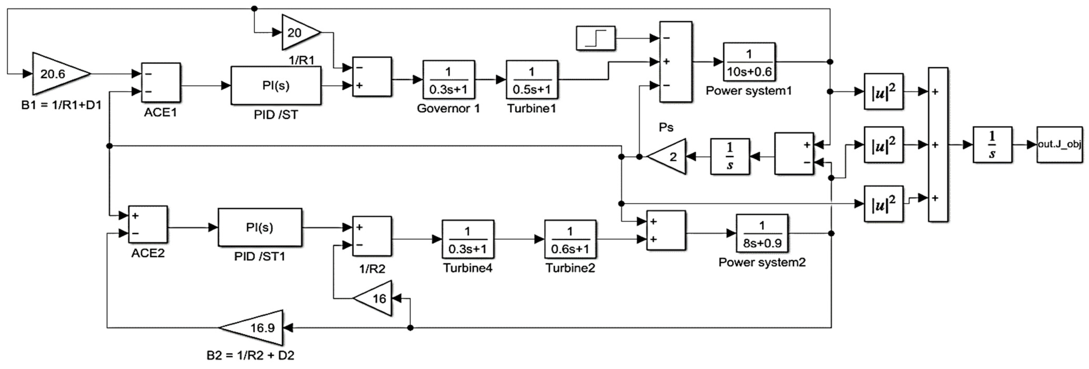
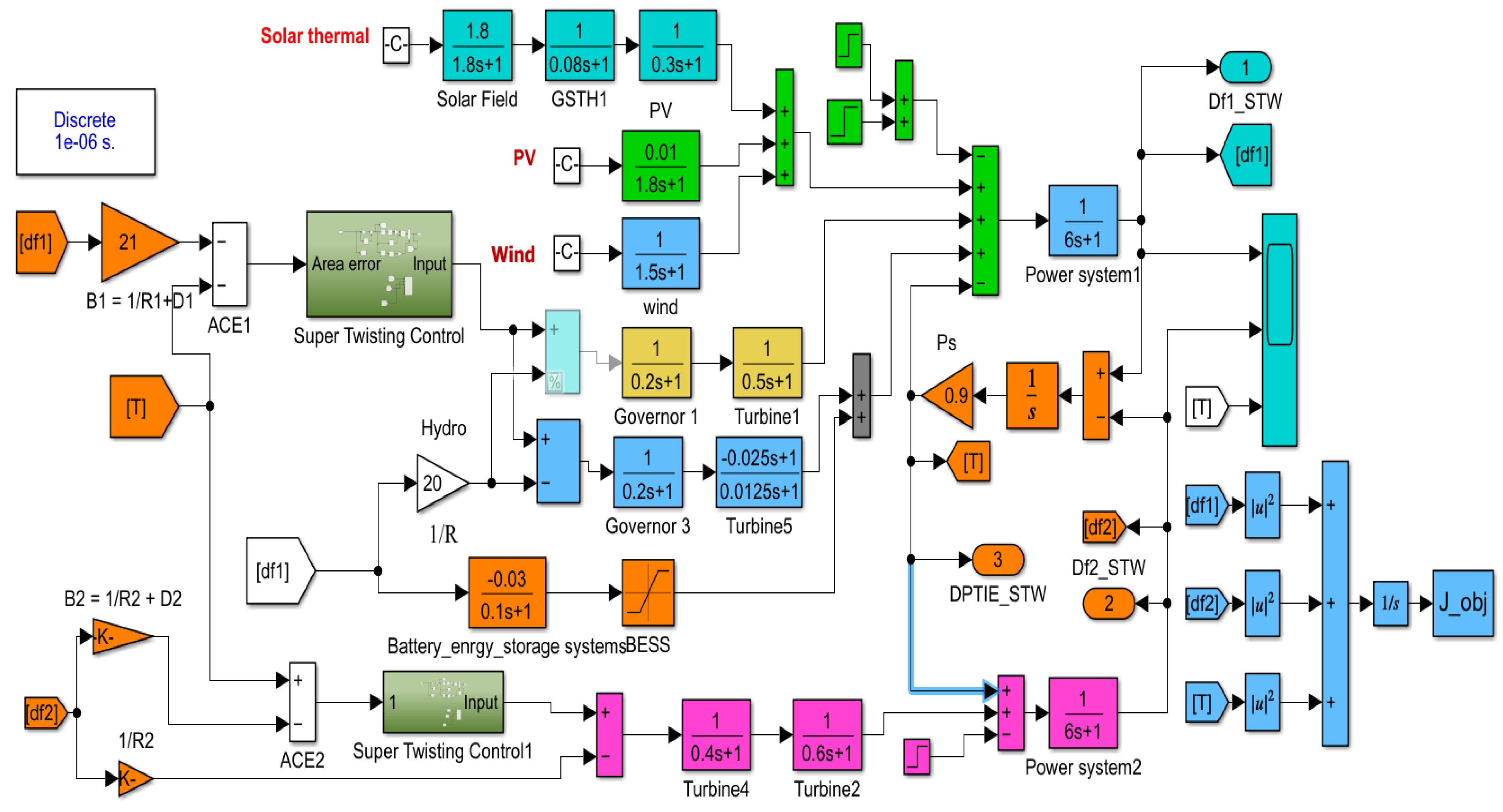
2. System Modelling

In this paper, a hybrid TAPS that contains different energy resources is studied; these energy resources are explained as follows.

2.1. Solar Thermal Power Plant

The cost of electrical energy generated from the sun is decreasing [36]. Currently, solar thermal (STH) power plants are broadly used to provide either heat energy or electrical energy. The commonly used devices in STH system can be classified into two types: The first is a linear collector, like a parabolic trough and Fresnel’s lenses, and the second is point-focused, like a parabolic dish and central tower. Solar radiation calculation is investigated by Abdelaal in [37,38]. The principle of operation of an STH plant depends on collecting the sun rays by the collectors and then reflecting the sun rays to the receiver, which contains a liquid (oil or molten salt). Therefore, the liquid temperature rises to an excessive value. The excessive temperature liquid interchanges the heat energy with water to provide super-heated steam that drives a turbine and then generates electrical power. The first stage of collecting sun rays, reflecting them, heating the liquid, and exchanging energy with water of the STH plant can be modelled by the following equation [39]:

$$G_s\left(s\right)=\frac{K_{STH}}{{\tau }_{STH}S+1}$$

(1)

where K_STH is the gain and ${\tau }_{STH}$ is the delay time of the first stage. The model of the speed governor (SG) and turbine is given by the following:

$$G_{GPT}\left(s\right)=\frac{K_{G\_STH}}{T_{G\_STH}S+1}$$

(2)

$$G_{TPT}\left(s\right)=\frac{K_{T\_STH}}{T_{T\_STH}S+1}$$

(3)

where T_{G_STH} and T_{T_STH} are the SG and turbine time delay, and K_{G_STH} and K_{T_STH} are the gain of the SG and turbine, respectively.

2.2. Photovoltaic Power Plant

When solar rays hit the solar cell (CS), photons hit electrons; as a result, electrons are freed, and electric current flows. The current is captured and transferred to wires; as a result, electrical energy is obtained. Electrical energy is supplied, provided that the light is incident on the CS. To work at the peak power of the CS, a maximum power point tracker should be used. Inverters are used to convert the energy to AC. The mathematical representation of the PV power plant is given by following equation [40]:

$$G_{PV}=\frac{K_{PV}}{{\tau }_{PV}s+1}$$

(4)

where τ_PV and $K_{PV}$ are the time delay and gain of the PV unit.

2.3. Wind Turbine Power Plant

The WT transforms energy contained in the wind to mechanical power, which is converted to electrical power. The output power is strongly affected by the wind speed. The WT can be modelled as follows [41]:

$$G_{WT}=\frac{\mathsf{\Delta }{P}_{WT}}{\mathsf{\Delta }{P}_{WT\_inp}}=\frac{K_{WT}}{1+{\tau }_{WT}s}$$

(5)

where ΔP_WT represents the change in the WT output power, $\mathsf{\Delta }{P}_{WT\_inp}$ represents the WT input power, and τ_WT and $K_{WT}$ are the time delay and gain of the WT power plant.

2.4. Hydro-Power Plant

The mathematical representation of the hydro-turbine and penstock could be represented by the following [42]:

$$G_{H\_T}=\frac{-T_{HT}s+1}{0.5T_{HT}s+1}$$

(6)

where $T_{H_T}$ represents the water delay time. The hydro-turbine SG is given by the following:

$$G_{H\_T\_G}=\frac{T_{R}s+1}{\left(T_{GHY}s+1\right)(T_{R}s+1)}$$

(7)

where T_R is the reset in time and T_GHY represents the governor delay time.

2.5. Battery Energy Storage System

The battery energy storage system (BESS) has an important impact in the case of high contribution of renewable energies, owing to weather variations. When there is a surplus in the generated power, the BESS absorbs energy and then releases it during a power decrease. The mathematical representation of the BESS is given by the following [43]:

$$G_B=\frac{K_B}{{\tau }_{B}s+1}$$

(8)

where K_B and τ_B are the BESS gain and time constants, respectively.

2.6. The Power System

The rotor dynamics of power system synchronous generators in both areas is represented by the following:

$$G_{PS}=\frac{1}{{\tau }_{PS}s+D}$$

(9)

where τ_PS is given by 2H, H represents the inertia of the machine, and D represents the coefficient of damping.

The governing equation of the speed governor and turbine are given as follows:

$$\frac{∆Y}{{\mathsf{\Delta }P}_{ref}-\frac{1}{R}\mathsf{\Delta }f}=\frac{1}{{\tau }_{SG}s+1}$$

(10)

$$G_{T\_DG}=\frac{1}{{\tau }_{T}s+1}$$

(11)

where ${\mathsf{\Delta }P}_{ref}$ is the reference input power, $\mathsf{\Delta }Y$ is the change in the governor controlling valve position, R is the speed regulation coefficient, Δf is the change in frequency, ${\tau }_{SG}$ is the SG delay time, and ${\tau }_T$ is the turbine delay time.

The constants of the suggested system are given in

Table 1. System parameters.

Plant Type	Parameters	Plant Type	Parameters
Solar Thermal	τS-TH = 1.8 s	Power system	H1 = H2 = 3 s
	KS-TH = 1.8		D1 = D2 = 1
	KG-STH = KT-STH = 1		R1 = R2 = 0.05 pu
	τT-STH = 0.3 s	BESS	KB = −0.003
PV	KPV = 1		TB = 0.1 s
	TPV = 1.8 s	Wind Turbine	KWT = 1
			TWT = 1.5 s

, where all data are found in [1,2,3].

3. Hippopotamus and One-to-One Based Optimizers

As mentioned in the introduction of this paper, metaheuristic techniques are used to LFC. For example, GA is used to tune fractional order PID controller in [44], while it is used to tune the gains of PID in [45]. HO and OOBO techniques have been realized for optimal estimation of the PI regulator for LFC of the TAPS. According to Amiri [46], HO has superior performance compared with other challenging heuristic optimizers, whereas, as stated by Dehghani [47], OOBO has an excellent convergence rate. Both techniques have been tested on numerous systems, and they have accurate results. More information about both optimizers can be found in [46,47].

Four performance indices can be utilized to measure the frequency error in PS. The first is the integral time weighted squared error (ITSE), the second is the integral time weighted absolute error (ITAE), the third is named the integral of square error (ISE), and the last one is the integral of absolute error (IAE). These four indices can be utilized as objective function (OF) for the heuristic optimizers; the most popular and commonly used is the ISE because of its high performance [48]. In the TAPS, this index is defined by the following:

$$OF={\int }_0^{t_f}\left[\mathsf{\Delta }{f}_1^2+\mathsf{\Delta }{f}_2^2+\mathsf{\Delta }{P}_{tie}^2\right]dt$$

(12)

where ∆f₁ and ∆f₂ are the frequency deviations in areas 1 and 2, respectively. ∆P_tie is the tie line deviation.

4. Sliding Mode Control and Super Twisting

SMC was suggested and implemented in 1950 in the Soviet Union by Utkins and Itkis [49]. During the last years, there is a noteworthy attention on SMC. SMC is a robust procedure since it is not sensitive to system parameter variation [50]. Due to its implementation simplicity, it has gained widespread use in many applications [51]. SMC can benefit to achieve specific favorite control performance [52]. There are two phases for implementing SMC, the reaching phase, in which the trajectory moves in the direction of the switching surface and arrives there in a finite amount of time, and the sliding phase, in which the state trajectories slide and stay on this surface, which is referred to as the sliding surface [34].

There are many versions of SMC. ST has a high-performance control and is easy to implement. There is a common problem that exists in all versions of SMC, which is the chattering problem due to the high switching speed of SMC [53]. All SMC techniques intend to direct the controlled system to a specified surface called the sliding surface. An important requirement for the sliding surface is that it must be constructed to achieve the desired control objectives [51].

4.1. Super Twisting Control Law

The control input could be written as follows:

$$u=c|S{|}^{\frac{1}{2}}sgn\left(S\right)+b\int sgn\left(S\right)dt$$

(13)

If the area control error for area 1 is e₁, then the sliding surface S is given as follows:

$$S={\dot{e}}_1+c{e}_1$$

(14)

The proper values of c₁ and b₁ are vital for the selection of the sliding surface. In this paper, the values of c₁ and b₁ are obtained by using the HO. The HO will tune the sliding surface to obtain the optimal values of c₁ and b₁.

4.2. Validation of the Proposed Scheme

In order to prove the high performance of the suggested technique, a simple TAPS model will be used. The block diagram of this system is shown in Figure 1, and the data are found in [54]. The three techniques (ST, HO, and OOBO) are tested using the test system, and the values of the ST, OBOO PI controller, and HO controller are given in

Table 2. Controller parameters.

Controller	Area 1		Area 2
	KP1 (or c1)	KI1 (or b1)	KP2 (or c2)	KI2 (or b2)
OBOO	0.4658	0.6468	1.2780	0
HO	0.4365	0.6465	1.0949	0.0820
ST	3.8341	31.1777	1.8890	0.3802

. The search space of the parameters of the PI controller ranges from 0 to 100; this range is decided after many trials to determine the stable region of the system. As noticed in Table 2, both OBOO and HO controller parameters have close values, which prove the accuracy of both methods. The frequency deviation in area 1 is shown in Figure 2, due to a step load change of 0.2 pu. As shown in Figure 2, the maximum overshoot (OS) in the case of ST is 1.4 × 10⁻³ pu, which is less than that obtained with the other methods, i.e., HO and OBOO controllers result in equal OS, which is 0.009 pu. The settling time is 7 s with ST, while it is 60 s with both HO and OBOO controllers. The drawback of the ST controller is the known chattering problem of the SMC.

Figure 3 shows the frequency deviation in area 2, which has similar explanations as in the case of area 1, to confirm that the ST has the lowest OS and the least settling time as compared to the other controllers. The tie line power in pu is shown in Figure 4. All the previous figures prove the high performance of the ST controller.

5. Simulation Results

The suggested system is simulated employing SIMULINK, and it is shown in Figure 5, where all parameters are given in the figure. The analysis is performed by applying a sudden change in the load of 0.20 pu in the first area at time t = 5 s, followed by another load change at t = 20 s.

To implement both the HO and OOBO, the number of iterations for both optimizers is taken as 25, whereas the population size is 50.

Table 3. Gains of the PI regulator.

Optimizer	Area One	Area Two	OF Value
HO	KP = 3.2998 KI = 6.2767	KP = 0.2770 KI = 0	3.8260 × 10−5
OOBO	KP = 3.6424 KI = 5.7919	KP = 0.0240 KI = 3.467 × 10−4	1.05 × 10−5

shows the PI controllers’ gains of both optimizers.

In the next section, different cases will be implemented to test the performance of ST, HO, and OOBO.

5.1. Case 1

In this event, the load in area 1 is suddenly raised by 0.2 pu at t = 5 s, and another load increase of 0.2 pu is applied at t = 20 s for a total 0.4 pu change in load power. As illustrated in Figure 6, the ST controller is capable of decaying any variation in frequency with almost zero state error. The maximum overshoot in frequency deviation in area 1 is less than 2 × 10⁻³ pu. Figure 7 demonstrates the deviation in frequency in area 2, which is very small and is less than 3 × 10⁻⁵ pu. Figure 8 shows the power variation in the tie line, which is also very small and is less than 6 × 10⁻⁴ pu. The previous figures verify the good performance of the ST regulator and its powerfulness for frequency and tie line power tunning.

For the sake of comparison with the ST controller, both OOBO and HO algorithms are used. The performance characteristics of the three controllers are given in Figure 9, Figure 10 and Figure 11. Figure 9 displays the frequency variations in area 1; the advantage of the ST regulator over both the HO and OOBO regulators is obvious in terms of overshoot, settling time, and steady-state error. Moreover, HO and OOBO have close response characteristics.

Figure 10 shows the frequency fluctuations in area 2 for the three regulators. The frequency deviation is almost zero in the case of ST, whereas there are some oscillations in the case of the OOBO and HO regulators. Figure 11 shows the deviation in tie line power in pu, which is very small.

Table 4. Case 1 system dynamic performance.

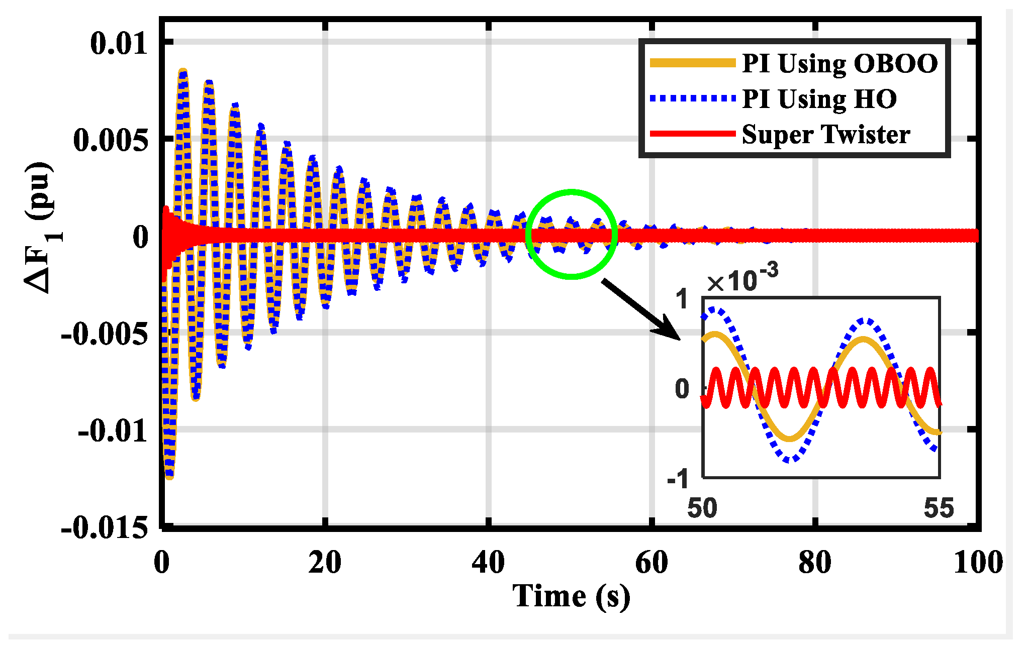
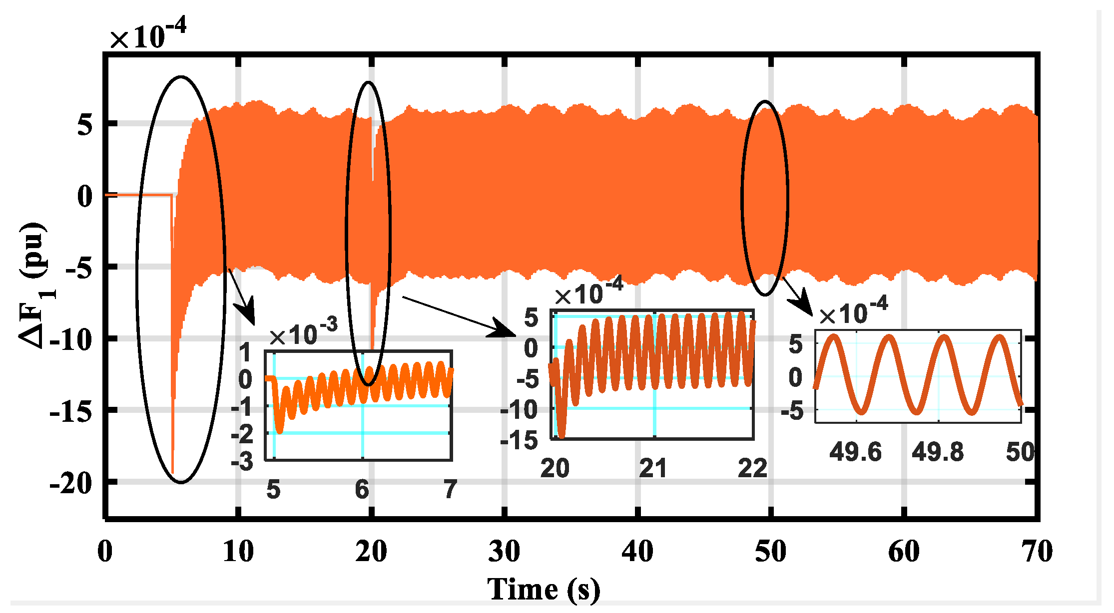
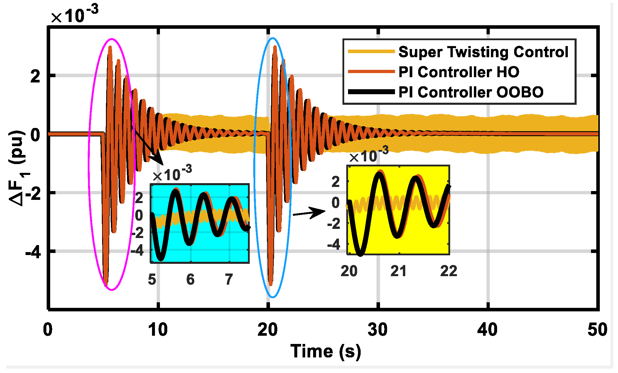
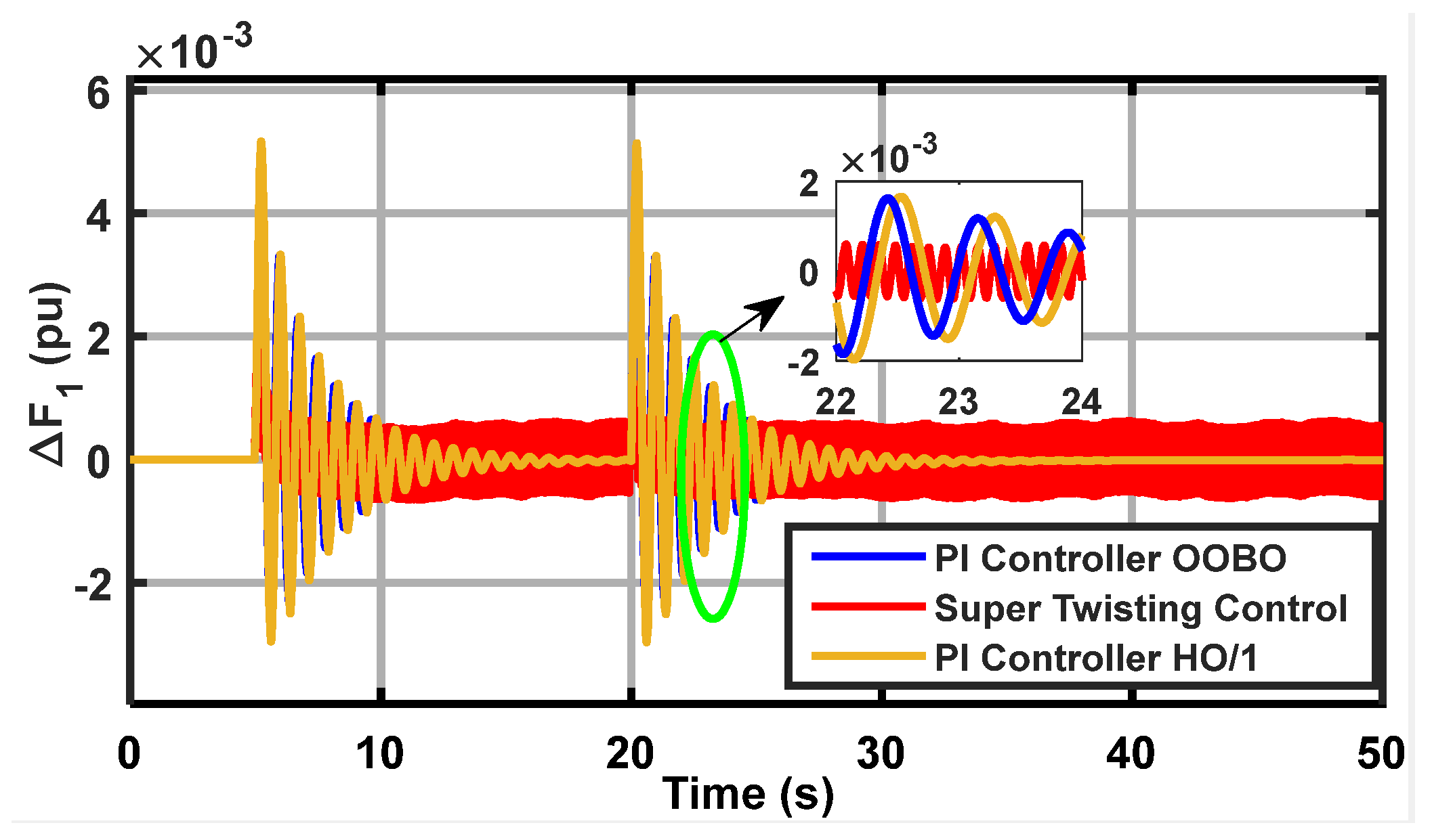
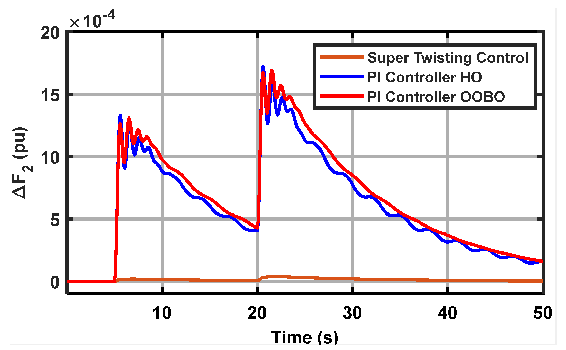
Optimizer	Area One (∆F1 pu)	Area Two (∆F2 pu)
HO	OS = −2.96 × 10−3 Ts = 19.5 s	OS = −1.422 × 10−3 Ts = 19.5 s
OOBO	OS = −2.6 × 10−3 Ts = 19.95 s	OS = −1.425 × 10−3 Ts = 19.95 s
ST	OS = −1.88 × 10−3 Ts = 6.6 s	OS = −2.48 × 10−5 Ts = 6.6 s

summarizes the dynamic performance in case 1 for a load disturbance of 0.2. The maximum overshoot (OS) in frequency deviation in area 1 is less than 3 × 10⁻⁵ pu. The 2% settling time (Ts) with the ST proposed method is 6.6 s, while it is 19.5 s with Ho and OOBO.

5.2. Case 2

In this case, the load in area 1 is abruptly decreased by 0.2 pu at t = 5 s, and another load decrease of 0.2 pu occurs at t = 20 s for a total 0.4 pu change in load power. The response is nearly comparable to the preceding case, and the responses of frequencies and tie line power with the TA are demonstrated in Figure 12, Figure 13 and Figure 14.

As illustrated by the previous figures, all the controllers can diminish any oscillations in frequency with almost zero state error. The OS in frequency deviation in area 1 is less than 3 × 10⁻⁵ pu. The Ts with the ST proposed method is 6.6 s in area 1 and 5.1 s in area 2, which is lower than that with HO and OOBO.

Table 5. Case 2 system dynamic performance.

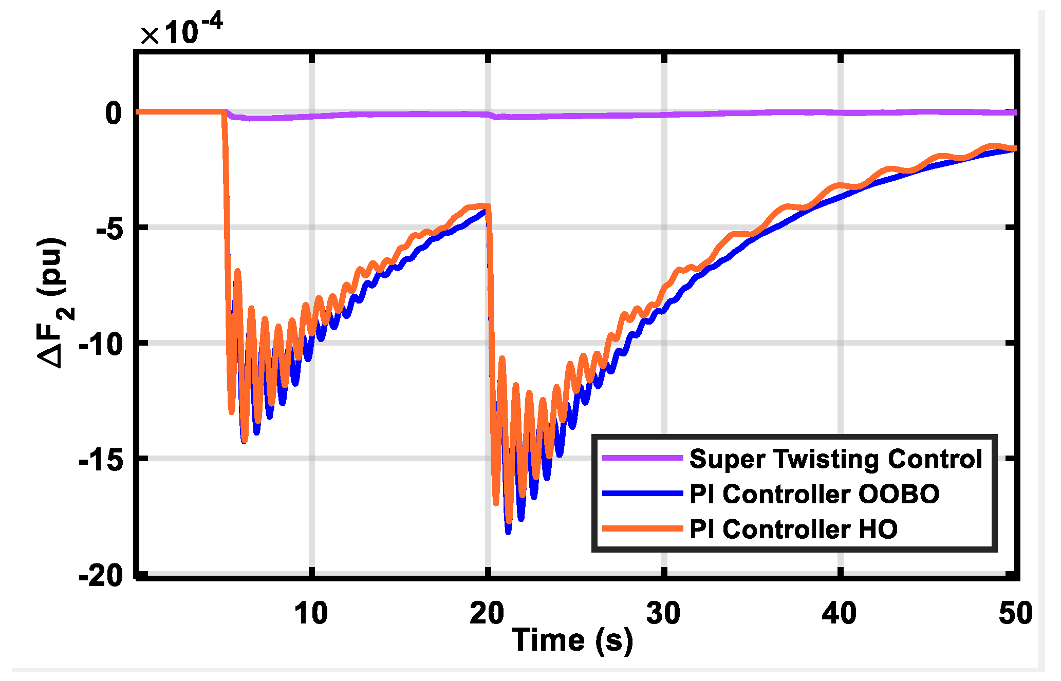
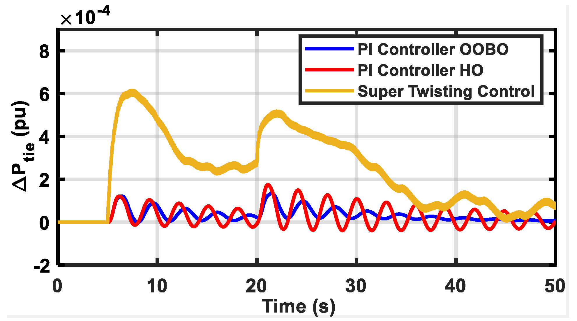
Optimizer	Area One (∆F1 pu)	Area Two (∆F2 pu)
HO	OS = −2.96 × 10−3 Ts = 19.5 s	OS = 1.33 × 10−3 Ts = 19.2 s
OOBO	OS = −2.6 × 10−3 Ts = 19.95 s	OS = 1.2635 × 10−3 Ts = 20 s
ST	OS = −1.88 × 10−3 Ts = 6.6 s	OS = 1.8 × 10−5 Ts = 5.1 s

summarizes the dynamic performance in case 2 regarding the OS and TS.

5.3. Case 3

The ST controller is robust for any change in parameters; therefore, in this case, the power system time constant will be changed from 3 to 5 s for an approximately 67% change in the time constant in the presence of the disturbance as in case 2. The responses are exhibited in Figure 15 and Figure 16. Figure 15 demonstrates the frequency response in area 1, and Figure 16 displays the frequency response in area 2. As observed in Figure 15 and Figure 16, the ST has a very small effect by the parameter variation, which is the main feature of SMC, where other controllers are strongly affected by the parameter change, especially during transient. The maximum overshoot is 0.9 × 10⁻³ in the case of ST, while it is approximately 4 × 10⁻³ in the case of the other controllers, which prove the fact that ST is not affected to any parameter change.

The proposed ST controller has a better performance regarding both OS and Ts as reported in

Table 6. Case 3 system dynamic performance.

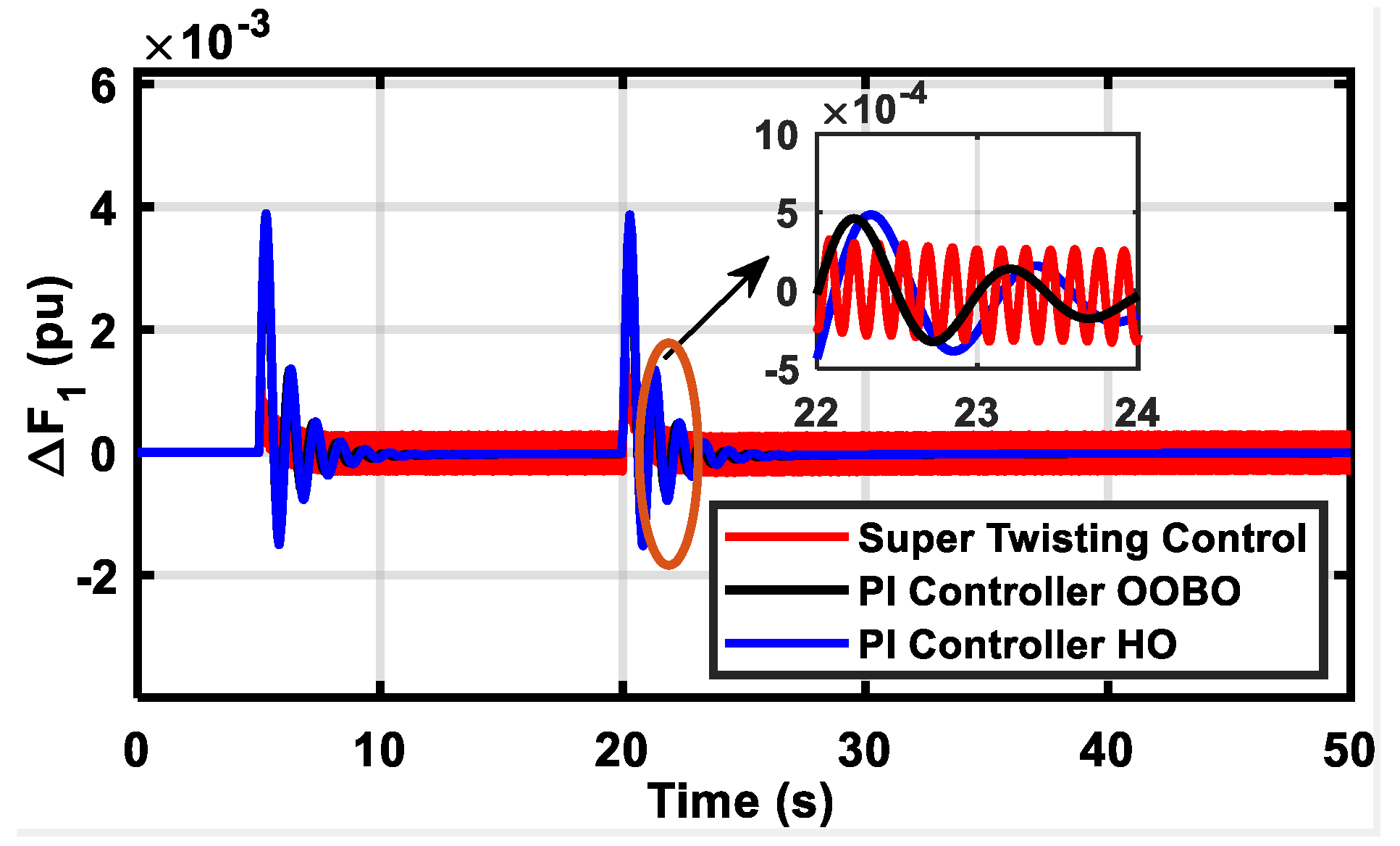
Optimizer	Area One (∆F1 pu)	Area Two (∆F2 pu)
HO	OS = 3.9 × 10−3 Ts = 11.4 s	OS = 1.332 × 10−3 Ts = 19.2 s
OOBO	OS = 3.77 × 10−3 Ts = 11.8 s	OS = 1.31 × 10−3 Ts = 20 s
ST	OS = 1.23 × 10−3 Ts = 6.2 s	OS = 5.5 × 10−5 Ts = 5.5 s

.

6. Conclusions

The goal of the present work is to use ST to control frequency in a TAPS with different energy sources with different dynamic characteristics. For the sake of comparison with the ST controller, two different controllers are used, OOBO and HO, to compute the optimal gains of the PI regulators. The optimal sliding surface for ST is obtained by both OOBO and HO, and the control law for ST is specified. The integral of square errors has been utilized as the OF to obtain the gains for both area controllers. Three cases are considered to test the performance of the three controllers. The first case is by increasing the demand in area 1 by 0.2 pu and another 0.2 pu at different times. The simulation results for this particular case show that the ST has a superior performance over the other controllers. Case 2 is by decreasing the load in area 1 by the same manner as in case 1, which has the same conclusion as the first case. Case 3 is by changing the time constant of the network. Case 3 proves that ST is not affected by parameter change, whereas other techniques are strongly affected by parameter change. Since only simple energy sources are considered in this paper, it is recommended that, for any future study, the exact models for each energy source should be considered.

References

- Ali, T.; Malik, S.A.; Daraz, A.; Adeel, M.; Aslam, S.; Herodotou, H. Load Frequency Control and Automatic Voltage Regulation in Four-Area Interconnected Power Systems Using a Gradient-Based Optimizer. Energies 2023, 16, 2086. [Google Scholar] [CrossRef]
- Grover, H.; Verma, A.; Bhatti, T.S. Load Frequency Control & Automatic Voltage Regulation for a Single Area Power System. In Proceedings of the 2020 IEEE 9th Power India International Conference (PIICON), Sonepat, India, 28 February–1 March 2020. [Google Scholar]
- Babu, N.R.; Bhagat, S.K.; Saikia, L.C.; Chiranjeevi, T.; Devarapalli, R.; Márquez, F.P.G. A Comprehensive Review of Recent Strategies on Automatic Generation Control/Load Frequency Control in Power Systems. Arch. Comput. Methods Eng. 2022, 30, 543–572. [Google Scholar] [CrossRef]
- Ranjan, M.; Shankar, R. A literature survey on load frequency control considering renewable energy integration in power system: Recent trends and future prospects. J. Energy Storage 2022, 45, 103717. [Google Scholar] [CrossRef]
- Sharma, D. Load Frequency Control: A Literature Review. Int. J. Sci. Technol. Res. 2020, 9, 6421–6437. [Google Scholar]
- Liu, X.; Qiao, S.; Liu, Z. A Survey on Load Frequency Control of Multi-Area Power Systems: Recent Challenges and Strategies. Energies 2023, 16, 2323. [Google Scholar] [CrossRef]
- Kumari, S.; Pathak, P.K. State-of-the-Art Review on Recent Load Frequency Control Architectures of Various Power System Configurations. Electr. Power Compon. Syst. 2024, 52, 722–765. [Google Scholar] [CrossRef]
- Sönmez, Ş.; Ayasun, S. Gain and phase margins based delay-dependent stability analysis of single-area load frequency control system with constant communication time delay. Trans. Inst. Meas. Control 2017, 40, 014233121769022. [Google Scholar] [CrossRef]
- Weldcherkos, T.; Salau, A.O.; Ashagrie, A. Modeling and design of an automatic generation control for hydropower plants using Neuro-Fuzzy controller. Energy Rep. 2021, 7, 6626–6637. [Google Scholar] [CrossRef]
- Sagar, P.S.V.; Swarup, K.S. Load frequency control in isolated micro-grids using centralized model predictive control. In Proceedings of the 2016 IEEE International Conference on Power Electronics, Drives and Energy Systems (PEDES), Trivandrum, India, 14–17 December 2016. [Google Scholar]
- Pathak, P.K.; Yadav, A.K.; Padmanaban, S.; Kamwa, I. Fractional Cascade LFC for Distributed Energy Sources via Advanced Optimization Technique under High Renewable Shares. IEEE Access 2022, 10, 92828–92842. [Google Scholar] [CrossRef]
- Elkasem, A.H.A.; Kamel, S.; Khamies, M.; Nasrat, L. Frequency regulation in a hybrid renewable power grid: An effective strategy utilizing load frequency control and redox flow batteries. Sci. Rep. 2024, 14, 9576. [Google Scholar] [CrossRef]
- Huang, C.; Yang, M.; Ge, H.; Deng, S.; Chen, C. DMPC-based load frequency control of multi-area power systems with heterogeneous energy storage system considering SoC consensus. Electr. Power Syst. Res. 2024, 228, 110064. [Google Scholar] [CrossRef]
- Fosha, C.E.; Elgerd, O.I. The Megawatt-Frequency Control Problem: A New Approach Via Optimal Control Theory. IEEE Trans. Power Appar. Syst. 1970, 89, 563–577. [Google Scholar] [CrossRef]
- Jagessar, D.R.; Dorile, P.O.; McCann, R.A. Design of a Linear Optimal Quadratic Regulator for Frequency Control in a Two-Area Deregulated Power Market. In Proceedings of the 2021 International Conference on Technology and Policy in Energy and Electric Power (ICT-PEP), Jakarta, Indonesia, 29–30 September 2021. [Google Scholar]
- Muthukumari, S.; Kanagalakshmi, S.; Kumar, T.K.S. Optimal Tuning of LQR for Load Frequency Control in Deregulated Power System for Given Time Domain Specifications. In Proceedings of the 2019 29th Australasian Universities Power Engineering Conference (AUPEC), Nadi, Fiji, 26–29 November 2019. [Google Scholar]
- Thenmalar, K. Fuzzy logic based load frequency control of power system. Mater. Today Proc. 2021, 45, 8170–8175. [Google Scholar]
- Kumar, N.K.; Gopi, R.S.; Kuppusamy, R.; Nikolovski, S.; Teekaraman, Y.; Vairavasundaram, I.; Venkateswarulu, S. Fuzzy Logic-Based Load Frequency Control in an Island Hybrid Power System Model Using Artificial Bee Colony Optimization. Energies 2022, 15, 2199. [Google Scholar] [CrossRef]
- Al-Majidi, S.D.; Al-Nussairi, M.K.; Mohammed, A.J.; Dakhil, A.M.; Abbod, M.F.; Al-Raweshidy, H.S. Design of a Load Frequency Controller Based on an Optimal Neural Network. Energies 2022, 15, 6223. [Google Scholar] [CrossRef]
- Mohseni, N.A.; Bayati, N. Robust Multi-Objective H2/H∞ Load Frequency Control of Multi-Area Interconnected Power Systems Using TS Fuzzy Modeling by Considering Delay and Uncertainty. Energies 2022, 15, 5525. [Google Scholar] [CrossRef]
- Sondhi, S.; Hote, Y.V. Fractional order PID controller for load frequency control. Energy Convers. Manag. 2014, 85, 343–353. [Google Scholar] [CrossRef]
- Ahmed, M.; Magdy, G.; Khamies, M.; Kamel, S. Modified TID controller for load frequency control of a two-area interconnected diverse-unit power system. Int. J. Electr. Power Energy Syst. 2022, 135, 107528. [Google Scholar] [CrossRef]
- Ogar, V.N.; Hussain, S.; Gamage, K.A.A. Load Frequency Control Using the Particle Swarm Optimisation Algorithm and PID Controller for Effective Monitoring of Transmission Line. Energies 2023, 16, 5748. [Google Scholar] [CrossRef]
- Daneshfar, F.; Bevrani, H. Load–Frequency Control: A GA-Based Multi-Agent Reinforcement Learning. IET Gener. Transm. Dis. 2010, 4, 13–26. [Google Scholar] [CrossRef]
- Ramjug-Ballgobin, R.; Ramlukon, C. A hybrid metaheuristic optimisation technique for load frequency control. SN Appl. Sci. 2021, 3, 547. [Google Scholar] [CrossRef]
- Alahakoon, S.; Roy, R.B.; Arachchillage, S.J. Optimizing Load Frequency Control in Standalone Marine Microgrids Using Meta-Heuristic Techniques. Energies 2023, 16, 4846. [Google Scholar] [CrossRef]
- Ahmed, M.; Mansor, M.; Feyad, H.; Taha, E.; Abdullah, G. An Optimal LFC in Two-Area Power Systems Using a Meta-heuristic Optimization Algorithm. Int. J. Electr. Comput. Eng. 2017, 7, 3217–3225. [Google Scholar]
- Dashtdar, M.; Flah, A.; Hosseinimoghadam, S.M.S.; El-Fergany, A. Frequency control of the islanded microgrid including energy storage using soft computing. Sci. Rep. 2022, 12, 20409. [Google Scholar] [CrossRef]
- El-Bahay, M.H.; Lotfy, M.E.; El-Hameed, M.A. Effective participation of wind turbines in frequency control of a two-area power system using coot optimization. Prot. Control Mod. Power Syst. 2023, 8, 14. [Google Scholar] [CrossRef]
- Sarath, P.S.K.; Monica, I.S. Application of BFOA in Two Area Load Frequency Control. Int. J. Eng. Technol. (UAE) 2018, 7, 50–54. [Google Scholar]
- Satheeshkumar, R.; Phd, S. Ant Lion Optimization Approach for Load Frequency Control of Multi-Area Interconnected Power Systems. Circuits Syst. 2016, 7, 2357–2383. [Google Scholar] [CrossRef]
- Mahmoud, G.; Chen, Y.; Zhang, L.; Li, M. Sliding Mode Based Nonlinear Load Frequency Control for Interconnected Coupling Power Network. Int. J. Control. Autom. Syst. 2022, 20, 3731–3739. [Google Scholar] [CrossRef]
- Kumar, A.; Anwar, N.; Kumar, S. Sliding mode controller design for frequency regulation in an interconnected power system. Prot. Control Mod. Power Syst. 2021, 6, 6. [Google Scholar] [CrossRef]
- Tran, A.-T.; Duong, M.P.; Pham, N.T.; Shim, J.W. Enhanced sliding mode controller design via meta-heuristic algorithm for robust and stable load frequency control in multi-area power systems. IET Gener. Transm. Distrib. 2024, 18, 460–478. [Google Scholar] [CrossRef]
- Nair, A.S.; Ezhilarasi, D. Performance Analysis of Super Twisting Sliding Mode Controller by ADAMS–MATLAB Co-simulation in Lower Extremity Exoskeleton. Int. J. Precis. Eng. Manuf.-Green Technol. 2020, 7, 743–754. [Google Scholar] [CrossRef]
- Abdelaal, A.K.; Mohamed, E.F.; El-Fergany, A.A. Optimal Scheduling of Hybrid Sustainable Energy Microgrid: A Case Study for a Resort in Sokhna, Egypt. Sustainability 2022, 14, 12948. [Google Scholar] [CrossRef]
- Abdelaal, A.K.; El-Fergany, A. Estimation of optimal tilt angles for photovoltaic panels in Egypt with experimental verifications. Sci. Rep. 2023, 13, 3268. [Google Scholar] [CrossRef]
- Abdelaal, A.K.; Alhamahmy, A.I.; Attia HE, D.; El-Fergany, A.A. Maximizing solar radiations of PV panels using artificial gorilla troops reinforced by experimental investigations. Sci. Rep. 2024, 14, 3562. [Google Scholar] [CrossRef]
- Fayek, H.H. Load Frequency Control of a Power System with 100% Renewables. In Proceedings of the 2019 54th International Universities Power Engineering Conference (UPEC), Bucharest, Romania, 3–6 September 2019. [Google Scholar]
- Lee, D.-J.; Wang, L. Small-Signal Stability Analysis of an Autonomous Hybrid Renewable Energy Power Generation/Energy Storage System Part I: Time-Domain Simulations. IEEE Trans. Energy Convers. 2008, 23, 311–320. [Google Scholar] [CrossRef]
- Ray, P.K.; Mohanty, S.R.; Kishor, N. Proportional–integral controller based small-signal analysis of hybrid distributed generation systems. Energy Convers. Manag. 2011, 52, 1943–1954. [Google Scholar] [CrossRef]
- Nanda, J.; Sharma, D.; Mishra, S. Performance analysis of automatic generation control of interconnected power systems with delayed mode operation of area control error. J. Eng. 2015, 2015, 164–173. [Google Scholar] [CrossRef]
- Kalyani, S.; Nagalakshmi, S.; Marisha, R. Load frequency control using battery energy storage system in interconnected power system. In Proceedings of the 2012 Third International Conference on Computing, Communication and Networking Technologies (ICCCNT’12), Coimbatore, India, 26–28 July 2012. [Google Scholar]
- Regad, M.; Helaimi, M.; Taleb, R.; Gabbar, H.A.; Othman, A.M. Fractional Order PID Control of Hybrid Power System with Renewable Generation Using Genetic Algorithm. In Proceedings of the 2019 IEEE 7th International Conference on Smart Energy Grid Engineering (SEGE), Oshawa, ON, Canada, 12–14 August 2019. [Google Scholar]
- Das, D.; Roy, A.K.; Sinha, N. Genetic Algorithm Based PI Controller for Frequency Control of an Autonomous Hybrid Generation System. In Proceedings of the international Multi Conference of Engineers and Computer Scientists IMECS 2011, Hong Kong, China, 16–18 March 2011; Volume 2. [Google Scholar]
- Amiri, M.H.; Hashjin, N.M.; Montazeri, M.; Mirjalili, S.; Khodadadi, N. Hippopotamus Optimization Algorithm: A Novel Nature-Inspired Optimization Algorithm. Sci. Rep. 2023, 14, 5032. [Google Scholar] [CrossRef]
- Dehghani, M.; Trojovská, E.; Trojovský, P.; Malik, O.P. OOBO: A New Metaheuristic Algorithm for Solving Optimization Problems. Biomimetics 2023, 8, 468. [Google Scholar] [CrossRef] [PubMed]
- Sahu, R.K.; Gorripotu, T.S.; Panda, S. Automatic generation control of multi-area power systems with diverse energy sources using Teaching Learning Based Optimization algorithm. Eng. Sci. Technol. Int. J. 2016, 19, 113–134. [Google Scholar] [CrossRef]
- Poznyak, A.S.; Orlov, Y.V.; Vadim, I. Utkin and sliding mode control. J. Frankl. Inst. 2023, 360, 12892–12921. [Google Scholar] [CrossRef]
- Gambhire, S.J.; Kishore, D.R.; Londhe, P.S.; Pawar, S.N. Review of sliding mode based control techniques for control system applications. Int. J. Dyn. Control 2021, 9, 363–378. [Google Scholar] [CrossRef]
- Komurcugil, H.; Biricik, S.; Bayhan, S.; Zhang, Z. Sliding Mode Control: Overview of Its Applications in Power Converters. IEEE Ind. Electron. Mag. 2021, 15, 40–49. [Google Scholar] [CrossRef]
- Dong, C.S.T.; Nguyen, Q.T.; Nguyen, D.Q.; Vo, H.H.; Tran, T.C.; Brandstetter, P. PMSM Drive with Sliding Mode Direct Torque Control. In AETA 2022—Recent Advances in Electrical Engineering and Related Sciences: Theory and Application; Springer Nature: Singapore, 2024. [Google Scholar]
- Utkin, V.; Lee, H. Chattering Problem in Sliding Mode Control Systems. In Proceedings of the International Workshop on Variable Structure Systems, 2006, VSS’06, Alghero, Italy, 5–7 June 2006. [Google Scholar]
- Saadat, H. Power System Analysis, 3rd ed.; PSA Publishing LLC: Williamsport, PA, USA, 2011. [Google Scholar]