
Order or Collaborate? Manufacturers Utilize 3D-Printed Parts to Sustainably Facilitate Increased Product Variety


Abstract
:1. Introduction
- (1)
- What conditions prompt the Manufacturer to adopt the Supplier’s 3DP technology to increase product variety?
- (2)
- If it is adopted, what is the better contract for the Manufacturer?
- (3)
- How does the cost savings from 3DP’s improved resource efficiency affect the equilibrium outcomes, and what management insights will it bring for sustainable production?
2. Literature Review
3. Model
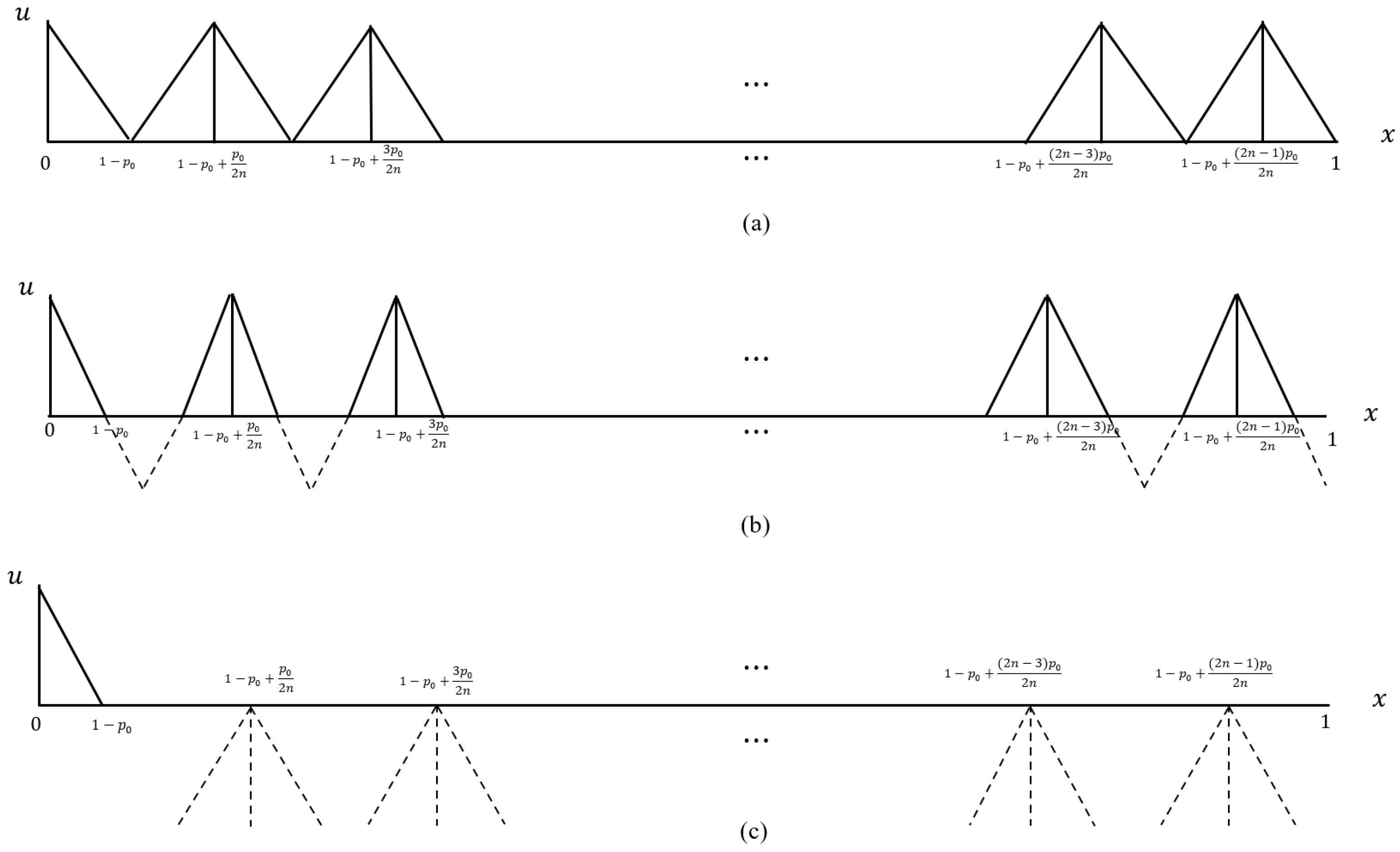
3.1. Consumer Utility and Product Variety
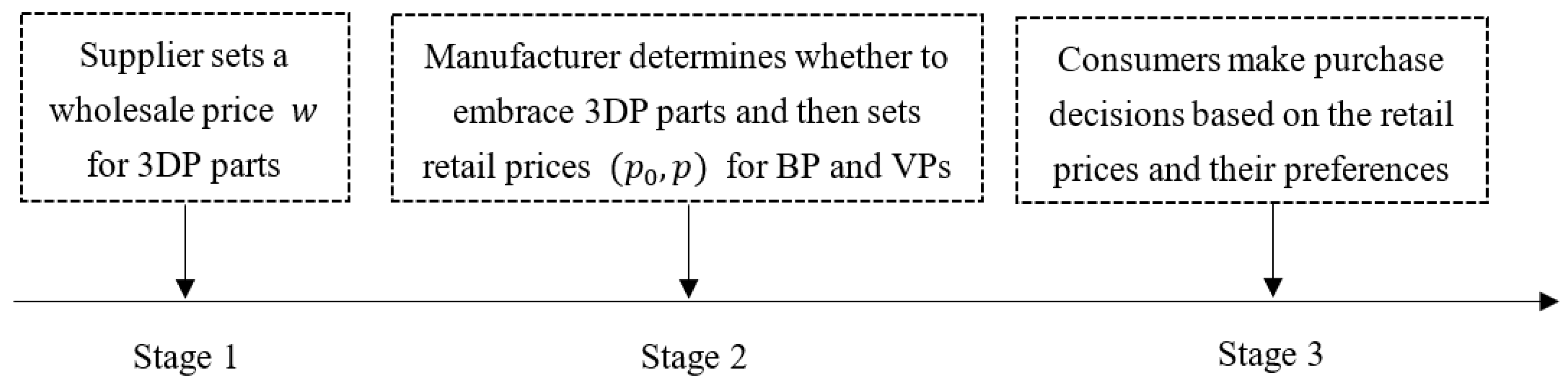
3.2. In the Ordering Model
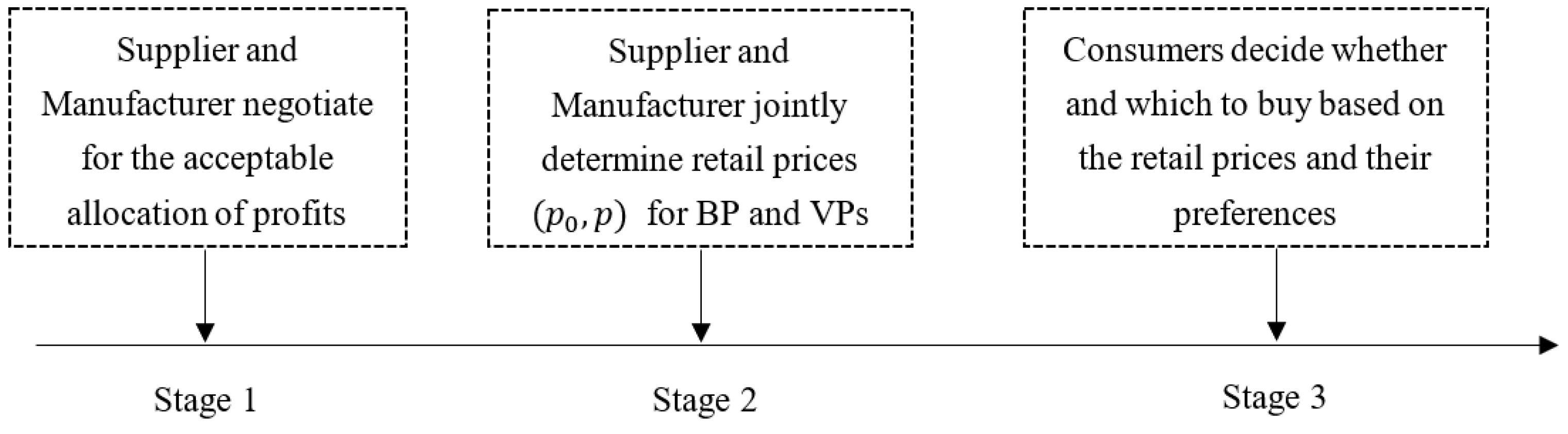
3.3. In the Collaboration Model
4. Equilibrium and Analysis
4.1. Equilibrium in the Ordering Model
- (i)
- When , ;
- (ii)
- When , ;
- (iii)
- When , for all ,
- where , , , and .
4.2. Equilibrium in the Collaboration Model
- (1)
- When , ;
- (2)
- When , ;
- (3)
- When , for all ,
- where and .
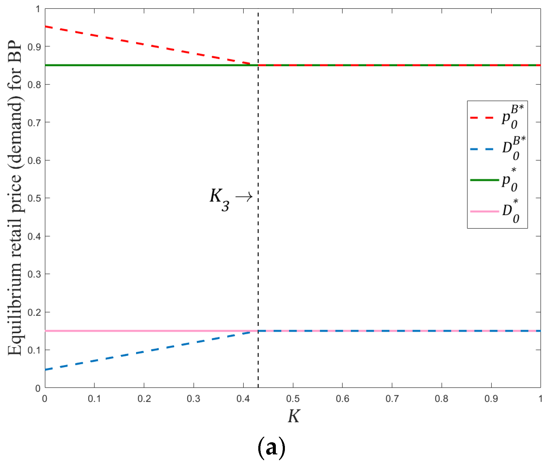
5. Comparison
6. Discussion
6.1. Main Findings
6.2. Practical Implications
6.3. Contributions to Literature
7. Conclusions and Future Research
7.1. Conclusions
7.2. Future Research
Author Contributions
Funding
Institutional Review Board Statement
Informed Consent Statement
Data Availability Statement
Acknowledgments
Conflicts of Interest
Appendix A
References
- O’Reilly, G. Wohlers Report 2023 Unveils Continued Double-Digit Growth. 2023. Available online: https://newsroom.astm.org/newsroom-articles/wohlers-report-2023-unveils-continued-double-digit-growth (accessed on 26 April 2024).
- Ghadge, A.; Karantoni, G.; Chaudhuri, A.; Srinivasan, A. Impact of additive manufacturing on aircraft supply chain performance: A system dynamics approach. J. Manuf. Technol. Manag. 2018, 29, 846–865. [Google Scholar] [CrossRef]
- Sun, L.; Hua, G.; Cheng, T.C.E.; Wang, Y. How to price 3D-printed products? Pricing strategy for 3D printing platforms. Int. J. Prod. Econ. 2020, 226, 107600. [Google Scholar] [CrossRef]
- Kunovjanek, M.; Knofius, N.; Reiner, G. Additive manufacturing and supply chains—A systematic review. Prod. Plan. Control 2022, 33, 1231–1251. [Google Scholar] [CrossRef]
- Choi, T.-M.; Kumar, S.; Yue, X.; Chan, H.-L. Disruptive technologies and operations management in the industry 4.0 era and beyond. Prod. Oper. Manag. 2022, 31, 9–31. [Google Scholar] [CrossRef]
- Weller, C.; Kleer, R.; Piller, F.T. Economic implications of 3D printing: Market structure models in light of additive manufacturing revisited. Int. J. Prod. Econ. 2015, 164, 43–56. [Google Scholar] [CrossRef]
- Gebler, M.; Schoot Uiterkamp, A.J.M.; Visser, C. A global sustainability perspective on 3D printing technologies. Energy Policy 2014, 74, 158–167. [Google Scholar] [CrossRef]
- Chekurov, S.; Metsä-Kortelainen, S.; Salmi, M.; Roda, I.; Jussila, A. The perceived value of additively manufactured digital spare parts in industry: An empirical investigation. Int. J. Prod. Econ. 2018, 205, 87–97. [Google Scholar] [CrossRef]
- Priyadarshini, J.; Kr Singh, R.; Mishra, R.; Chaudhuri, A.; Kamble, S. Supply chain resilience and improving sustainability through additive manufacturing implementation: A systematic literature review and framework. Prod. Plan. Control 2023. Published online. [Google Scholar] [CrossRef]
- Long, Y.; Pan, J.; Zhang, Q.; Hao, Y. 3D printing technology and its impact on Chinese manufacturing. Int. J. Prod. Res. 2017, 55, 1488–1497. [Google Scholar] [CrossRef]
- Wheeler, A. Stratasys Produces 3D Printed Parts for New Airbus Aircraft. 2015. Available online: https://www.engineering.com/story/stratasys-produces-3d-printed-parts-for-new-airbus-aircraft (accessed on 26 April 2024).
- Limer, E. Boeing Is Putting 3-D-Printed Titanium Parts in the 787 Dreamliner. 2017. Available online: https://www.popularmechanics.com/flight/airlines/a26018/boeing-printed-titanium/ (accessed on 26 April 2024).
- Jordan, M. Can Nike Use 3D-Printing to Sustainably Mass Customize Its Offer to Consumers? 2017. Available online: https://d3.harvard.edu/platform-rctom/submission/can-nike-use-3d-printing-to-sustainably-mass-customize-its-offer-to-consumers/ (accessed on 26 April 2024).
- Jia, F.; Wang, X.; Mustafee, N.; Hao, L. Investigating the feasibility of supply chain-centric business models in 3D chocolate printing: A simulation study. Technol. Forecast. Soc. Change 2016, 102, 202–213. [Google Scholar] [CrossRef]
- Arbabian, M.E.; Wagner, M.R. The impact of 3D printing on manufacturer–retailer supply chains. Eur. J. Oper. Res. 2020, 285, 538–552. [Google Scholar] [CrossRef]
- Arbabian, M.E. Supply chain coordination via additive manufacturing. Int. J. Prod. Econ. 2022, 243, 108318. [Google Scholar] [CrossRef]
- Xiong, Y.; Lu, H.; Li, G.-D.; Xia, S.-M.; Wang, Z.-X.; Xu, Y.-F. Game changer or threat: The impact of 3D printing on the logistics supplier circular supply chain. Ind. Mark. Manag. 2022, 106, 461–475. [Google Scholar] [CrossRef]
- Tong, M.; Li, W. Remanufacturing model selection with 3D printing. Comput. Ind. Eng. 2023, 183, 109529. [Google Scholar] [CrossRef]
- Li, W.; Sun, H.; Tong, M.; Mustafee, N.; Koh, L. Customizing customization in a 3D printing-enabled hybrid manufacturing supply chain. Int. J. Prod. Econ. 2024, 268, 109103. [Google Scholar] [CrossRef]
- Sun, M.; To Ng, C.; Yang, L.; Zhang, T. Optimal after-sales service offering strategy: Additive manufacturing, traditional manufacturing, or hybrid? Int. J. Prod. Econ. 2024, 268, 109116. [Google Scholar] [CrossRef]
- Chen, L.; Cui, Y.; Lee, H.L. Retailing with 3D printing. Prod. Oper. Manag. 2021, 30, 1986–2007. [Google Scholar] [CrossRef]
- Guo, S.; Choi, T.-M.; Chung, S.-H. Self-design fun: Should 3D printing be employed in mass customization operations? Eur. J. Oper. Res. 2022, 299, 889–897. [Google Scholar] [CrossRef]
- Sethuraman, N.; Parlaktürk, A.K.; Swaminathan, J.M. Personal fabrication as an operational strategy: Value of delegating production to customer using 3D printing. Prod. Oper. Manag. 2023, 32, 2362–2375. [Google Scholar] [CrossRef]
- Sun, L.; Hua, G.; Cheng, T.C.E.; Teunter, R.H.; Dong, J.; Wang, Y. Purchase or rent? Optimal pricing for 3D printing capacity sharing platforms. Eur. J. Oper. Res. 2023, 307, 1192–1205. [Google Scholar] [CrossRef]
- Hartl, R.F.; Kort, P.M. Possible market entry of a firm with an additive manufacturing technology. Int. J. Prod. Econ. 2017, 194, 190–199. [Google Scholar] [CrossRef]
- Kleer, R.; Piller, F.T. Local manufacturing and structural shifts in competition: Market dynamics of additive manufacturing. Int. J. Prod. Econ. 2019, 216, 23–34. [Google Scholar] [CrossRef]
- Nie, J.; Xu, X.; Yue, X.; Guo, Q.; Zhou, Y. Less is more: A strategic analysis of 3D printing with limited capacity. Int. J. Prod. Econ. 2023, 258, 108816. [Google Scholar] [CrossRef]
- Feng, Q.; Lu, L.X. The strategic perils of low cost outsourcing. Manag. Sci. 2012, 58, 1196–1210. [Google Scholar] [CrossRef]
- Zhang, Q.; Zhang, J.; Tang, W. Coordinating a supply chain with green innovation in a dynamic setting. 4OR-Q. J. Oper. Res. 2017, 15, 133–162. [Google Scholar] [CrossRef]
- Zhou, Y.; Bao, M.; Chen, X.; Xu, X. Co-op advertising and emission reduction cost sharing contracts and coordination in low-carbon supply chain based on fairness concerns. J. Clean. Prod. 2016, 133, 402–413. [Google Scholar] [CrossRef]
- Guan, Z.; Ye, T.; Yin, R. Channel coordination under Nash bargaining fairness concerns in differential games of goodwill accumulation. Eur. J. Oper. Res. 2020, 285, 916–930. [Google Scholar] [CrossRef]
- Shi, X.; Chan, H.L.; Dong, C. Value of bargaining contract in a supply chain system with sustainability investment: An incentive analysis. IEEE Trans. Syst. Man Cybern. Syst. 2020, 50, 1622–1634. [Google Scholar] [CrossRef]
- Du, X.; Jiang, S.; Tao, S.; Wang, S. Cooperative advertising and coordination in a supply chain: The role of Nash bargaining fairness concerns. RAIRO Oper. Res. 2024, 58, 1–18. [Google Scholar] [CrossRef]
- Tirole, J. The Theory of Industrial Organization; MIT Press: Cambridge, MA, USA, 1988; pp. 174–176. [Google Scholar]
- Alptekinoğlu, A.; Corbett, C.J. Mass customization vs. mass production: Variety and price competition. Manuf. Serv. Oper. Manag. 2008, 10, 204–217. [Google Scholar] [CrossRef]
- Xiao, T.; Choi, T.-M.; Cheng, T.C.E. Optimal variety and pricing decisions of a supply chain with economies of scope. IEEE Trans. Eng. Manag. 2015, 62, 411–420. [Google Scholar] [CrossRef]
- Raz, G.; Druehl, C.T.; Blass, V. Design for the environment: Life-cycle approach using a Newsvendor model. Prod. Oper. Manag. 2013, 22, 940–957. [Google Scholar] [CrossRef]
- Zhao, Q.; Chen, W.; Liu, M. The impact of three-dimensional printing technology investment on a low-carbon manufacturing supply chain, investigated through the Stackelberg game. Int. J. Technol. Manag. 2024, 95, 120–155. [Google Scholar] [CrossRef]
- Knight, P. How 3D Printing Is Changing the Way Nike Approaches Production and Innovation. 2018. Available online: https://d3.harvard.edu/platform-rctom/submission/how-3d-printing-is-changing-the-way-nike-approaches-production-and-innovation/ (accessed on 4 June 2024).
- Hanaphy, P. Adidas Reveals Futurecraft Strung, the “Ultimate” 3D Printed Running Shoe. 2020. Available online: https://3dprintingindustry.com/news/adidas-reveals-futurecraft-strung-the-ultimate-3d-printed-running-shoe-177073/ (accessed on 4 June 2024).
- Verry, P. Adidas Takes 3D Printing to a New Level with 4DFWD. 2021. Available online: https://footwearnews.com/shoes/outdoor-footwear/adidas-4dfwd-release-info-3d-printed-shoe-1203137591/ (accessed on 4 June 2024).
- Zhou, H.; Benton, W.C. Supply chain practice and information sharing. J. Oper. Manag. 2007, 25, 1348–1365. [Google Scholar] [CrossRef]
- Chu, W.H.J.; Lee, C.C. Strategic information sharing in a supply chain. Eur. J. Oper. Res. 2006, 174, 1567–1579. [Google Scholar] [CrossRef]


| Symbol | Description |
|---|---|
| x | |
| v | Consumer’s valuations for the base product and variety of products and normalized to 1 |
| u | Consumer net utility from buy one unit product |
| n | Supplier’s printing variety |
| K | Nature of cost savings of each 3DP part due to 3DP’s enhanced resource efficiency |
| θ | Bargaining power of the Manufacturer |
| Unit cost and total costs | |
| w | Wholesale price of 3DP parts |
| π | Profit function |
| m | This subscript represents the traditional manufacturer |
| s | This subscript represents the 3DP supplier |
| B | This superscript represents the Nash bargaining contract |
| Conditions | ||
|---|---|---|
| Conditions | ||
|---|---|---|
Disclaimer/Publisher’s Note: The statements, opinions and data contained in all publications are solely those of the individual author(s) and contributor(s) and not of MDPI and/or the editor(s). MDPI and/or the editor(s) disclaim responsibility for any injury to people or property resulting from any ideas, methods, instructions or products referred to in the content. |
© 2024 by the authors. Licensee MDPI, Basel, Switzerland. This article is an open access article distributed under the terms and conditions of the Creative Commons Attribution (CC BY) license (https://creativecommons.org/licenses/by/4.0/).
Share and Cite
Zhao, Q.; Wang, Z.; Zheng, K. Order or Collaborate? Manufacturers Utilize 3D-Printed Parts to Sustainably Facilitate Increased Product Variety. Sustainability 2024, 16, 5561. https://doi.org/10.3390/su16135561
Zhao Q, Wang Z, Zheng K. Order or Collaborate? Manufacturers Utilize 3D-Printed Parts to Sustainably Facilitate Increased Product Variety. Sustainability. 2024; 16(13):5561. https://doi.org/10.3390/su16135561
Chicago/Turabian StyleZhao, Qian, Zhengkai Wang, and Kaiming Zheng. 2024. "Order or Collaborate? Manufacturers Utilize 3D-Printed Parts to Sustainably Facilitate Increased Product Variety" Sustainability 16, no. 13: 5561. https://doi.org/10.3390/su16135561