Prediction on Demand for Regional Online Car-Hailing Travel Based on Self-Attention Memory and ConvLSTM

Abstract

High precision in forecasting travel demand for online car-hailing is crucial for traffic management to schedule vehicles, hence reducing energy consumption and achieving sustainable development. Netflix demand forecasting relies on the capture of spatiotemporal correlations. To extract the spatiotemporal information more fully, this study designs and develops a novel spatiotemporal prediction model with multidimensional inputs (MSACL) by embedding a self-attention memory (SAM) module into a convolutional long short-term memory neural network (ConvLSTM). The SAM module can extract features with long-range spatiotemporal dependencies. The experimental data are derived from the Chengdu City online car-hailing trajectory data set and the external factors data set. Comparative experiments demonstrate that the proposed model has higher accuracy. The proposed model outperforms the Sa-ConvLSTM model and has the highest prediction accuracy, shows a reduction in the mean absolute error (MAE) by 1.72, a reduction in the mean squared error (MSE) by 0.43, and an increase in the R-squared (R²) by 4%. In addition, ablation experiments illustrate the effectiveness of each component, where the external factor inputs have the least impact on the model accuracy, but the removal of the SAM module results in the most significant decrease in model accuracy.

1. Introduction

The development of internet technology has led to a significant change in the transport industry, one of the products of which is online car-hailing [1,2]. Online car-hailing refers to the business activity of constructing a service platform based on internet technology and using qualified vehicles and drivers to provide passengers with booked hire car services. The emergence of online car-hailing has influenced reducing carbon emissions. Due to the Chinese government’s efforts to reduce environmental pollution, many cities have limited the use of online car-hailing to electric energy as a power source. Compared with the previous use of oil as a power source, pollution emissions have been reduced to a certain extent, which is conducive to the sustainable development of society.

1.1. Trends in the Development of Online Car-Hailing

In 2012, online car-hailing rapidly swept through most Chinese cities. According to relevant data, as of June 2023, the number of users for online car-hailing in China had reached 472 million. The rapid development of online car-hailing services has brought great benefits to passengers and drivers, as well as businesses and society. However, it has also introduced new challenges, including an imbalance between supply and demand. Accurate forecasting of traveling demand for online car-hailing is an effective method to alleviate the supply–demand imbalance problem. By forecasting travel demand, data can provide support to online car-hailing drivers and management platforms. This guidance helps drivers navigate to hotspots, thereby alleviating the supply–demand balance issue.

1.2. Related Work

Previous research in the domain of online car-hailing has focused on predicting travel demand [3,4], analyzing factors affecting passenger flow [5,6,7], and carpooling strategies [8,9]. These studies have emphasized the importance of online car-hailing as a mode of transport. Therefore, accurately predicting the demand for online car-hailing is an important task for meeting the transportation needs of online car-hailing passengers.

Short-term demand forecasting for online car-hailing is a typical traffic forecasting problem. Researchers have classified traffic prediction into traffic flow prediction, journey time prediction, and speed prediction based on the different prediction objects [10], and according to the different research methods, they are mainly divided into prediction models based on linear system theory [11,12], prediction models based on nonlinear system theory [10,13], and neural network prediction models [14,15]. Compared to other models, neural network prediction models are popular because they have higher prediction accuracy. Therefore, we focus on designing neural network prediction models in our study.

In terms of time series prediction, Bi et al. [16] incorporated rainfall and whether it was a weekday into the gate recurrent unit (GRU) model, used K-fold cross-optimization of the model parameters, and found through evaluation of the metrics that the optimized GRU had a higher prediction accuracy. Ye et al. [4] combined the attention mechanism and the LSTM model, extracting multidimensional features to achieve demand prediction for online car-hailing traveling. Ye et al. [17] used a wide range of combined models for an extensive collapsing table to achieve demand prediction. Jiang et al. [18] proposed a least-squares support vector machine, which achieves high prediction accuracy and efficiency at the same time. To reduce the effect of data noise on model accuracy, Liu et al. [19] proposed an enhanced empirical mode decomposition long short-term memory neural network (EMD-LSTM) model. Compared with the model without noise reduction, the accuracy of their model is significantly improved.

In recent years, the development of various technologies has made it possible to forecast time series. To a certain extent, spatiotemporal sequence forecasting is more practical than time series sequence forecasting, and therefore has received more attention from researchers. Lu et al. [20] converted the 2D spatiotemporal attributes of the data into 2D images and input them into the ConvLSTM model. Ke et al. [21] extracted more temporal features by combining with the LSTM model and verified its validity. Wang et al. [22] constructed three time series of proximity, cycle, and trend, and used three ConvLSTM modules to further improve the prediction performance. Ge et al. [23] constructed a self-attention memory convolutional long short-term memory neural network (Sa-ConvLSTM) by inlaying the self-attentive memory module in the ConvLSTM model to further improve the prediction performance. Guo et al. [24] built a deep residual spatiotemporal network (RSTN) for spatiotemporal prediction using multisource data, and further improved the prediction performance by introducing dynamic request vectors. Like Guo’s study, Zhang et al. [25] utilized the deep spatiotemporal residual convolutional networks (DSTRNs) model to capture spatiotemporal information features. They also extracted external features using fully connected layers and integrated these with the spatiotemporal features to achieve promising prediction outcomes. Online car-hailing is an important way for tourists to get around. Based on multisource data, Liu et al. [26] developed a sophisticated approach to identifying travel patterns. They introduced the novel concept of service dependency degree and integrated it with a Bayesian optimization–enhanced long short-term memory–convolutional neural network (BO-LSTM-CNN) method. This innovative technique is employed for multitask forecasting of online car-hailing demand, offering a comprehensive and nuanced prediction model. Ye et al. [27] improved the accuracy of their model by combining an attention mechanism and a temporal convolutional network (TCN) to obtain more temporal information.

1.3. Contributions and Structure of This Paper

The demand for online car-hailing travel has emerged as a prominent research focus in recent times, with extensive scholarly inquiry. Despite the prevalent application of attention mechanisms in this field, they have predominantly been utilized to establish rudimentary connections. As a result, the combinatorial models developed through such an approach often fall short in capturing the intricate long-term spatiotemporal dependencies essential for accurate forecasting. Furthermore, the demand for online car-hailing travel exhibits distinct spatiotemporal characteristics and patterns of periodicity, aspects that have been overlooked in most existing studies. This oversight is notable, given the potential of these features to enhance the depth and accuracy of travel demand analysis.

Taking these shortcomings as a starting point, we conducted targeted research to address them. Specifically, the contributions of this paper are listed as follows:

(1)

To obtain long-term spatiotemporal dependence, Sa-ConvLSTM was used as the basic structure instead of a simple attention mechanism and ConvLSTM for connection.

(2)

We constructed a multi-input spatiotemporal prediction model (MSACL) using SA-ConvLSTM as the basic structure. Its inputs include multidimensional spatiotemporal series as well as external factor time series.

The rest of the paper is organized as follows. Section 2 provides a description and definition of the problem. Section 3 describes the methodology used for this study. Section 4 analyzes the results of the models. Section 5 draws the conclusions of the paper and the outlook.

2. Preliminaries

2.1. Defining

In order to introduce this study clearly, we define the demand for online car-hailing travel as follows: Demand for online car-hailing is the number of trips taken by residents of the region by online car-hailing in each period.

It should be noted that the demand here does not include the demand for trips that are made only with the intention of traveling by online car-hailing without the actual act of traveling.

2.2. Description of the Problem

Assuming that the current day is $d$ and the current time period is $t$, we can obtain the characteristics of the demand for online car-hailing in the current region as $x_d^t$. In the region, the demand for online car-hailing $x_d^{t-t_c+1}$ in the past $t_c$ time periods can be expressed as $x_d^t=\left\{x_d^{t-t_c+1},x_d^{t-t_c+2}\dots x_d^t\right\}$. The online car-hailing demand in the $d-1$ day time period can be defined as $x_{d-1}^t$, and the online car-hailing demand in the past $d-t_p$ day time period $t$ can be represented by $x_{d-t_p}^t$. The online car-hailing traveling demand shows a certain cyclicity, so we constructed a spatiotemporal sequence $x_d^{t,period}$ reflecting the change law of its cyclicity. The demand for online car-hailing traveling is affected by the previous multiple time periods, so similarly we construct a spatiotemporal sequence $x_d^{t,close}$ reflecting the change pattern of the recent online car-hailing traveling demand, which can be expressed by the following two equations:

$$x_d^{t,period}=\left\{\begin{array}{ccc}{x}_{d-t_p}^{t+1}& \cdots & x_{d-t_p}^{t+n}\\ ⋮& \ddots & ⋮\\ x_{d-1}^{t+1}& \cdots & x_{d-1}^{t+n}\end{array}\right\}$$

(1)

$$x_d^{t,close}=\left\{x_d^{t-t_c+1}\dots x_d^t\right\}$$

(2)

Similarly, we can obtain the time series for each of the two external factors as

$$e_d^{t,period}=\left\{\begin{array}{ccc}{e}_{d-t_p}^{t+1}& \cdots & e_{d-t_p}^{t+n}\\ ⋮& \ddots & ⋮\\ e_{d-1}^{t+1}& \cdots & e_{d-1}^{t+n}\end{array}\right\}$$

(3)

$$e_d^{t,close}=\left(e_d^{t-t_c+1}\cdots e_d^t\right)$$

(4)

For the future $t+1$ time period in which the demand for online car-hailing is to be predicted as $x_d^{t+1}$, the demand for online car-hailing in the predicted $t+n$ time period can be defined as follows, since it is a multistep prediction in this study:

$$x_d^{t,future}=\left\{x_d^{t+1},x_d^{t+2}\cdots x_d^{t+n}\right\}$$

(5)

Based on the above discussion, the research problem can be formulated as finding a function $f$, through which the mapping of the spatiotemporal sequence of online car-hailing traveling demand and the time series of external factors to the online car-hailing traveling demand at multiple future time periods $x_d^{t,future}$ can be achieved, which can be expressed by the following equation:

$$f:\left\{x_d^{t,period},x_d^{t,close},e_d^{t,period},e_d^{t,close}\right\}\to x_d^{t,future}$$

(6)

3. Methodology

3.1. ConvLSTM

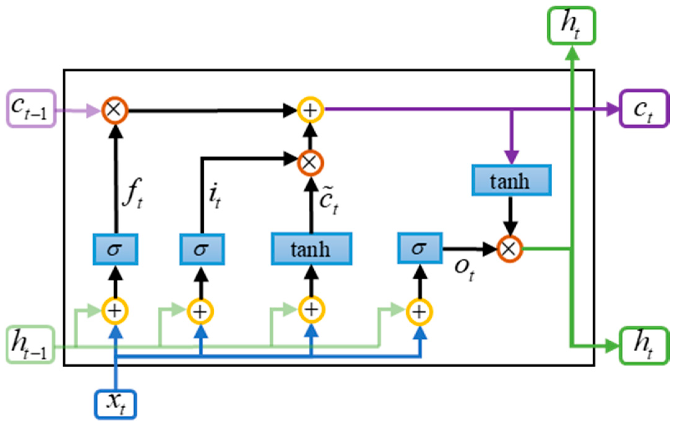
The traditional recurrent neural network (RNN) model yields good results in time series prediction due to its unique chain structure. However, when it comes to long sequence problems, the parameter sharing among its different units can lead to gradient explosion or vanishing, which in turn can cause nonconvergence. To solve this problem, Sepp Hochreiter and Jürgen Schmidhuber [28] proposed the LSTM model based on an RNN. Each LSTM cell consists of the four following components: a forgetting gate, an input gate, an output gate, and a memory cell. The structure is shown in Figure 1. The parameters of LSTM are separated rather than shared among the cells. In this case, the gradient vanishing and gradient explosion problems are solved.

Although LSTM can handle the time series prediction problem better, it is more difficult to handle the spatial correlation problem. In other words, LSTM is able to complete the time series prediction problem, but it is unable to do anything about the spatiotemporal prediction problem. Therefore, some scholars proposed the ConvLSTM model to deal with the spatiotemporal prediction problem, where ConvLSTM converts the multiplication operation in LSTM into a convolution operation. The improved ConvLSTM not only deals with 1-dimensional time series prediction problems, but also deals with 2D spatiotemporal prediction problems, which makes the model more applicable. Initially, ConvLSTM was used for rainfall prediction (i.e., to predict whether rain will fall in a region at a future moment and its intensity) [29], and it is also widely used in the field of transport.

The first is the forgetting gate, which determines what information was forgotten in the past. By reading the output of the previous cell $h_{ t-1}$ and the input of the current cell $x_{ t}$, each element is converted to a value of 0–1 by a sigmoid function. It is calculated using the following formula [28,29]:

$$f_{ t}=\sigma \left(W_{ f}\ast x_{ t}+U_{ f}\ast h_{ t-1}+b_{ f}\right)$$

(7)

where both $W_{ f}$ and $U_{ f}$ denote the weight matrix, $b_{ f}$ is the bias vectors, and $\sigma$ denotes the sigmoid activation function.

The input gate determines what new information will be stored in the cell state. It consists of two parts. The first is the selective update, which decides which parts to update by using the sigmoid function. The other part is the candidate layer, which uses the tanh function to generate new candidate values that may be added to the cell state $c_{ t}$ [28,29]

$$i_{ t}=\sigma \left(W_{ i}\ast x_{ t}+U_{ i}\ast h_{ t-1}+b_{ i}\right)$$

(8)

$${\tilde{c}}_{ t}=\tanh \left(W_{ c}\ast x_{ t}+U_{ c}\ast h_{ t-1}+b_{ c}\right)$$

(9)

where $W_i$, $U_i$, $W_c$, and $U_c$ are the weights and $b_i$ and $b_c$ denote the bias vectors.

Then there is the cell state update, which updates the cell state by combining the results of the forgetting gate and the input gate [28,29]

$$c_{ t}=f_{ t}\odot c_{ t-1}+i_{ t}\odot {\tilde{c}}_{ t}$$

(10)

Finally, there is the output gate, which decides which information in the cell state should be passed on to the hidden state at the next moment or as model output at the current moment. The activation value of the output gate is computed from the current input $x_{ t}$ and the hidden state of the previous cell $h_{ t-1}$ by a fully connected layer with a sigmoid activation function, and is then elementwise multiplied by the value of the cell state after the tanh function to obtain the final state $h_{ t}$ [28,29]

$$o_{ t}=\sigma \left(W_{ o}\ast x_{ t}+U_{ o}\ast h_{ t-1}+b_{ o}\right)$$

(11)

$$h_{ t}=o_{ t}\odot \tanh \left(c_{ t}\right)$$

(12)

where $W_o$ and $U_o$ are the weights, $b_{ \mathrm{o}}$ denotes the bias vectors, and $\odot$ is the Hadamard product, denoting the matrix multiplication by elements.

3.2. Sa-ConvLSTM

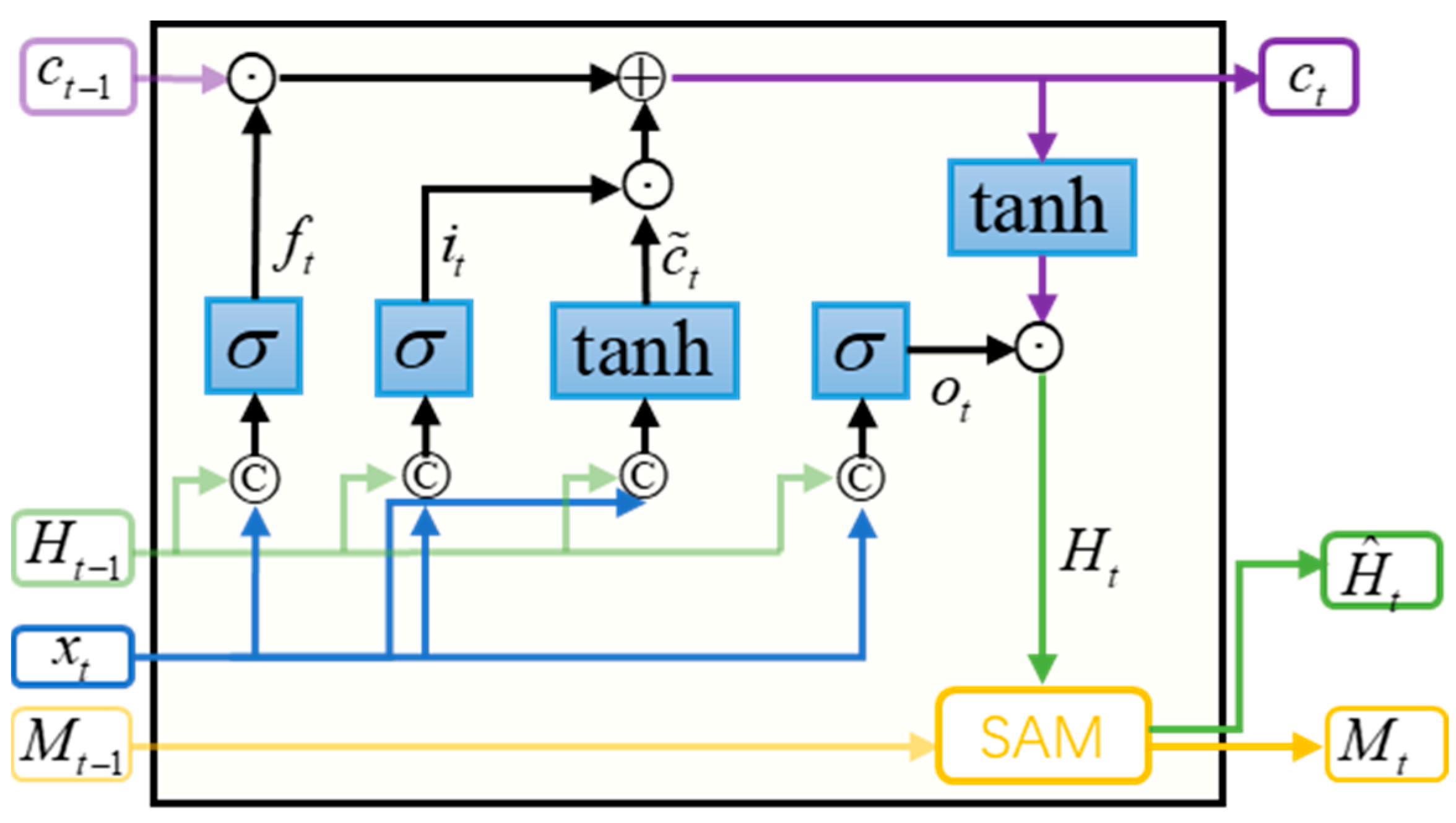
Sa-ConvLSTM was proposed in 2020 [30]. The traditional ConvLSTM can only acquire a small range of spatial relations, and the size of the range is determined by the size of the convolutional kernel. To extract a larger range of spatial correlations, one can only increase the number of convolution kernels or stack more ConvLSTM layers. Increasing the size of the convolutional kernel inevitably leads to a significant increase in computational load, which is detrimental to the stacking of model depth. Moreover, stacking additional layers of ConvLSTM tends to perform poorly. In this case, Sa-ConvLSTM introduces the self-attention mechanism into ConvLSTM, enabling global correlation capture with fewer layers. Sa-ConvLSTM does not simply inlay the self-attention mechanism into the model, but rather optimizes the self-attention mechanism further to obtain the memory-based self-attention memory (SAM) module. The SAM module is embedded into the model, and its structure is shown in Figure 2. From the figure, we can see that compared with the ConvLSTM model, the Sa-ConvLSTM model has an extra SAM module, which realizes the updating of the memory cells and the output feature maps of the current time step. Compared with the ConvLSTM model, the Sa-ConvLSTM model not only obtains the long-term spatiotemporal dependence through adaptive updating, but also extracts the global spatial dependence to a certain extent through the self-attention module. If this module is removed, the Sa-ConvLSTM model will become a ConvLSTM model.

The specific structure of the SAM module is shown in Figure 3. The input of this structure contains two inputs, which are the input feature map $H_t$ of the current time step and the output of the memory cell $M_{t-1}$ of the previous time step, and the capture of long-term spatial dependencies is accomplished according to the three parts of feature aggregation, memory updating, and outputs, and the final outputs are the memory cell $M_t$ of the current time and the final output of the current time step ${\widehat{H}}_t$ [30].

In the feature aggregation step, similar to the self-attention mechanism, the output $H_t$ of the current time step and the memory cell $M_{t-1}$ of the previous unit are projected to $Z_h$ and $Z_m$, and the aggregated features are obtained after splicing and convolution.

First, the query $Q_H$, the key $K_H$, and the value $V_H$ of the initial feature map $H_t$, and the key $K_M$ and the value $V_M$ of the memory cell $M_{t-1}$ can be computed by the following equations [23]:

$$Q_H=W_{hq}{H}_t\in {ℝ}^{\widehat{C}\times N}$$

(13)

$$K_H=W_{hk}{H}_t\in {ℝ}^{\widehat{C}\times N}$$

(14)

$$V_H=W_{hv}{H}_t\in {ℝ}^{C\times N}$$

(15)

$$K_M=W_{mk}{M}_{t-1}\in {ℝ}^{\widehat{C}\times N}$$

(16)

$$V_M=W_{mv}{M}_{t-1}\in {ℝ}^{\widehat{C}\times N}$$

(17)

In these equations, $W_{hq}$, $W_{hk}$, $W_{hv}$, $W_{mk}$, and $W_{mv}$ denote 1 × 1 convolutions.

Query $Q$ and key $K$ are multiplied to obtain similarity scores, which indicate the relevance of the current position to other positions [23,30]

$$e_h=Q_h^T{K}_h\in {ℝ}^{N\times N}$$

(18)

$$e_m=Q_h^T{K}_m\in {ℝ}^{N\times N}$$

(19)

Based on these proposed equations, the similarity scores calculation of different positions of feature map $H_t$ and the similarity scores calculation of different positions of memory cell $M_{t-1}$ can be simplified by using the following two formulas:

$$e_{h;i,j}=\left(H_{t,i}^T{W}_{hq}^T\right)\left(W_{hk}{H}_{t,j}\right),i,j\in \left\{1,2,\dots ,N\right\}.$$

(20)

$$e_{m;i,j}=\left(H_{t,i}^T{W}_{mq}^T\right)\left(W_{mk}{H}_{t,j}\right),i,j\in \left\{1,2,\dots ,N\right\}.$$

(21)

Next, the similarity scores $e_{h;i,j}$ and $e_{m;i,j}$ are input into the softmax function to obtain the attention weights ${\alpha }_{h; i,j}$ and ${\alpha }_{m; i,j}$. The softmax function converts the raw scores into a probability distribution such that the sum of the attention weights for all positions is 1. The formula is as follows [31]:

$${\alpha }_{h; i,j}=\frac{\exp e_{h; i,j}}{{\displaystyle {\sum }_{k=1}^N\exp e_{h; i,k}}}$$

(22)

$${\alpha }_{m; i,j}=\frac{\exp e_{m; i,j}}{{\displaystyle {\sum }_{k=1}^N\exp e_{m; i,k}}}$$

(23)

The aggregated feature for the $i$th position is derived by multiplying the attention score weighting with the corresponding $V$ [31]

$$Z_{h,i}={\displaystyle \sum _{j=1}^N{\alpha }_{h; i,j}{V}_{h;j}}={\displaystyle \sum _{j=1}^N{\alpha }_{\mathrm{h} i,j}{W}_{mv}{H}_{t;j}}$$

(24)

$$Z_{m,i}={\displaystyle \sum _{j=1}^N{\alpha }_{m; i,j}{V}_{M;j}}={\displaystyle \sum _{j=1}^N{\alpha }_{m; i,j}{W}_{mv}{M}_{t-1;j}}$$

(25)

The final aggregated features are obtained by splicing $Z_h$ and $Z_m$, computing them by 1 × 1 convolution

$$Z=W_Z\left[Z_h;Z_m\right]$$

(26)

After feature aggregation, the memory unit $M_{t-1}$ needs to be updated. The memory update module enables the SAM module to capture long-range dependencies in both spatial and temporal domains. By aggregating the feature $Z$ and current time step output $H_{ t}$, the memory unit $M_{t-1}$ is updated using a gating mechanism similar to that of LSTM, which can be expressed as follows [23,30]:

$$i_t^{\prime }=\sigma \left(W_{ m;\mathrm{z}i}\ast Z+W_{ m;hi}\ast H_{ t}+b_{ m;i}\right)$$

(27)

$$g_t^{\prime }=\tanh \left(W_{ m;zg}\ast Z+W_{ m;hg}\ast H_{ t}+b_{ m;\mathrm{g}}\right)$$

(28)

$$M_t=\left(1-i_t^{\prime }\right)\odot M_{t-1}+i_t^{\prime }\odot g_t^{\prime }$$

(29)

where $W_{ m;\mathrm{z}i}$, $W_{ m;hi}$, $W_{ m;zg}$, and $W_{ m;hg}$ denote the weight matrix and $b_{ m;i}$ and $b_{ m;\mathrm{g}}$ denote the bias. As $i_t^{\prime }$ gets closer to 0, it means that more information was left in the previous cell.

The final output is obtained by combining the updated memory cell $M_t$ with the output gates $o_t^{\prime }$ of the SAM module [23,30]

$$o_t^{\prime }=\sigma \left(W_{ m;\mathrm{zo}}\ast Z+W_{ m;ho}\ast H_{ t}+b_{ m;o}\right)$$

(30)

$${\widehat{H}}_t=o_t^{\prime }\odot M_t$$

(31)

where $W_{ m;\mathrm{zo}}$ and $W_{ m;ho}$ denote the weight matrix and $b_{ m;o}$ denotes the bias.

The Sa-ConvLSTM model is obtained by embedding the SAM module into the ConvLSTM model, and its computational procedure is shown below. Equations (32), (33), and (40) represent the operations of the SAM module [23,30].

Equations (32) and (33) represent the feature maps ${\widehat{H}}_{t-1}$ and memory information $M_{t-1}$ obtained after the SAM module for $H_{t-1}$ and $M_{t-1}$, respectively,

$${\widehat{H}}_{t-1}=SA\left(H_{t-1}\right)$$

(32)

$$M_t=SA\left(M_{t-1}\right)$$

(33)

where SA represents the operation of the SAM module.

Equations (34)–(39) represent the operations of the ConvLTSM model by simply replacing $H_{t-1}$ with ${\widehat{H}}_{t-1}$

$$f_{ t}=\sigma \left(W_{ f}\ast x_{ t}+U_{ f}\ast {\widehat{H}}_{t-1}+b_{ f}\right)$$

(34)

$$i_{ t}=\sigma \left(W_{ i}\ast x_{ t}+U_{ i}\ast {\widehat{H}}_{t-1}+b_{ i}\right)$$

(35)

$$o_{ t}=\sigma \left(W_{ o}\ast x_{ t}+U_{ o}\ast {\widehat{H}}_{t-1}+b_{ o}\right)$$

(36)

$${\tilde{c}}_{ t}=\tanh \left(W_{ c}\ast x_{ t}+U_{ c}\ast {\widehat{H}}_{t-1}+b_{ c}\right)$$

(37)

$$c_{ t}=f_{ t}\odot c_{ t-1}+i_{ t}\odot {\tilde{c}}_{ t}$$

(38)

$$H_t=o_{ t}\odot \tanh \left(c_{ t}\right)$$

(39)

In Equation (40), ${\widehat{H}}_t$ indicates that the final feature map output is obtained

$${\widehat{H}}_t=SA\left(H_t\right)$$

(40)

3.3. Proposed Model

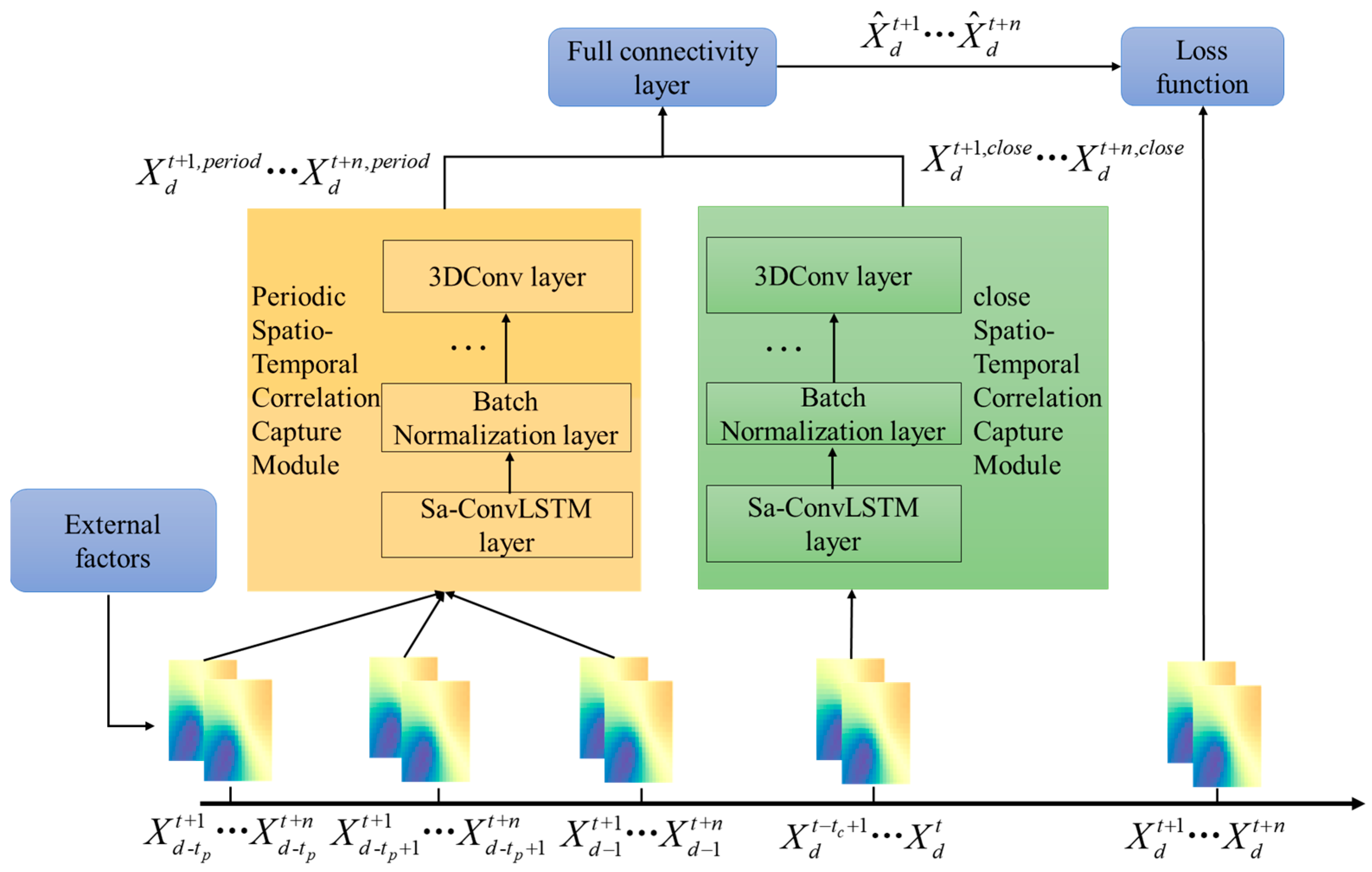
In this section, the proposed model will be presented and Figure 4 shows the main structure of the model, divided into three inputs, three modules, and the final output.

First, the input consists of three parts, which are the external factor time series $e_d^t$, the spatiotemporal series reflecting the change pattern of cyclical net travel demand $x_d^{t,period}$ and the spatiotemporal series reflecting the change pattern of recent net travel demand $x_d^{t,close}$, and the short-term cyclical spatiotemporal correlation capture module and the recent spatiotemporal correlation capture module accepts them, respectively, as $x_d^{t,period}$, $e_d^{t,period}$, $e_d^{t,close}$, and $x_d^{t,close}$. These two modules learn the internal spatiotemporal features present in them and output the outputs $\left\{x_d^{t+1,period}\dots x_d^{t+n,period}\right\}$ and $\left\{x_d^{t+1,close}\dots x_d^{t+n,close}\right\}$, respectively, which are combined, and output $\left\{x_d^{t+1}\dots x_d^{t+n}\right\}$ through the fully connected layer.

To match the spatiotemporal series, we extend the external factor time series $e_d^t\in {ℝ}^3$ into a spatiotemporal series $e_d^t\in {ℝ}^{3*I*J}$. Due to the limitations of the data available, it is not possible to determine the information on the external factors for a specific region, and we assume that there is no spatial variation in the factors. The inputs to the model can be expressed as

$$X_d^{t,period}=\left(x_d^{t,period},e_d^{t,period}\right)$$

(41)

$$X_d^{t,close}=\left(x_d^{t,close},e_d^{t,close}\right)$$

(42)

For subsequent ease of representation, we use $X^{period}$ and $X^{close}$ to simply denote $X_d^{t,period}$ and $X_d^{t,close}$.

The periodic spatiotemporal correlation capture module and the near-term spatiotemporal correlation capture module receive two inputs, respectively, and are dropped into the 2DSa-ConvLSTM layer. It can be simply expressed by the following equations:

$$X_{conv}^{period}=2DSaConvLSTM\left(X^{period}\right)$$

(43)

$$X_{conv}^{close}=2DSaConvLSTM\left(X^{close}\right)$$

(44)

To prevent overfitting problems, a batch normalization (BN) layer is added after each 2DSa-ConvLSTM layer. As an example, in the periodic spatiotemporal correlation capture module, the upper output $X_{conv}^{period}$ is normalized and $X_{conv}^{period}$ is forced to transform into a distribution with mean 0 and variance 1. After normalization, two learnable parameters, ${\gamma }_l$ and ${\beta }_l$, were introduced to adaptively adjust the normalized data [32]

$$X_N^{period}=\frac{X_{conv}^{period}-E\left(X_{conv}^{period}\right)}{\sqrt{Var\left(X_{conv}^{period}\right)}}$$

(45)

$$X_{BN}^{period}={\gamma }_l{X}_N^{period}+{\beta }_l$$

(46)

where $E\left(·\right)$ indicates the mean and $Var\left(·\right)$ means the variance.

After several layers of the 2DSa-ConvLSTM layer and the batch normalization layer, a C convolutional layer is used in the last layer of these two modules to output the prediction. The computational formula is as follows:

$$X_{3Dconv}^{period}=\sigma \left({\displaystyle \sum _{c=0}^{C-1}{\displaystyle \sum _{h=0}^{H-1}{\displaystyle \sum _{w=0}^{W-1}{w}_l^{c,h,w}{X}_{BN}^{period}+b_l}}}\right)$$

(47)

In this equation, $C$, $H$, and $W$ denote the length, width, and height of the convolution kernel, respectively, and $w_l$ and $b_l$ denote the weights and biases.

In the prediction module, the output is made by weighted fusion of the higher-order representations of the outputs of the two modules through a fully connected layer. It is computed as follows:

$$X_d^{t+i}=X_{3Dconv}^{period}{W}_{period}+X_{3Dconv}^{close}{W}_{close}$$

(48)

The loss function uses mean squared error (MSE), which is the most used of the regression loss functions and is the mean of the sum of squares of the errors

$$L\left(\Theta \right)=\frac{1}{n}{{\displaystyle \sum _{i=1}^n{\displaystyle \sum _{t=1}^T\left(x_i^t-{\widehat{x}}_i^t\right)}}}^2$$

(49)

where $T$ is the total number of predictions, $n$ is the step size of the prediction, and $\Theta$ is the set of learnable parameters.

4. Experiment

4.1. Data Sets

The data set used in the experiments is a real online car-hailing data set from Chengdu, China. The data set was provided by DiDi and contains online car-hailing journey trajectory data from 1 November to 30 November 2016 [33]. Examples of the original online car-hailing trajectory data are shown in

Table 1. Sample table of the online car-hailing trajectory data set.

Driver ID	Order ID	Timestamp	Longitude	Latitude
******	******	1477969149	104.0749	30.73734

****** represents the driver id and order id after information desensitization processing.

, and the first and second columns are desensitized to prevent personal information leakage.

The external factors data set used in this study primarily consists of rainfall, temperature, and whether it is a working day or not. The rainfall and temperature data were obtained from the National Meteorological Science Data Centre. Due to data issues, we make a basic assumption that both weather and temperature are consistent across different regional locations within the study area. In addition, whether it is a working day or not affects the distribution and changes in the demand for online car rental, so we add an indicator of whether it is a working day or not to our data set. We use a binary variable to indicate whether it is a working day or not, using “0” to indicate a nonworking day and “1” to indicate a working day. An example of the data is shown in

Table 2. An example of external factors.

Time	Quantity of Rainfall	Average Temperatures	Whether It Is a Working Day
1 November 2016 0:00:00	0.0	17.8	0

.

4.2. Evaluation Indicators

To assess the prediction accuracy of different models, this study selects mean absolute error (MAE), MSE, and R² (R-squared). The formulas are as follows [34,35]:

$$\mathrm{MAE}=\frac{1}{T}{\displaystyle \sum _{t=1}^T\left|{\widehat{y}}_t-y_t\right|}$$

(50)

$$\mathrm{MSE}=\frac{1}{T}{\displaystyle \sum _{t=1}^T{\left({\widehat{y}}_t-y_t\right)}^2}$$

(51)

$${\mathrm{R}}^2=1-\frac{{\displaystyle \sum _{i=1}^n{\left({\widehat{y}}_i-y_i\right)}^2}}{{\displaystyle \sum _{i=1}^n{\left(\frac{1}{n}{\displaystyle \sum _{i=1}^n{y}_i}-{\widehat{y}}_i\right)}^2}}$$

(52)

where $T$ denotes the total number of samples, $\widehat{y}$ represents the predicted value, and $y$ expresses the true value.

MAE is the mean of the absolute errors, ranging from 0 to infinity. The smaller the value, the better the prediction. Like MAE, MSE has a value ranging from 0 to positive infinity, and the larger the error, the larger the value of MSE. However, MSE is more affected by outliers than MAE.

R² generally ranges from 0 to 1. The closer the R² value is to 1, the better the prediction. If the R² value is 0, it means that every prediction of the sample is equal to the mean, which is the same as the mean model. If the R² value is less than 0, it means that the constructed model is not as good as the mean model.

4.3. Training Configuration

The experimental setting for this study is shown in

Table 3. Experimental environment.

Projects	Version and Parameters
CPU Version	12 vCPU Inter Xeon ® Platinum 8255C CPU @2.50 Ghz
GPU Version	RTX 3080
Number of GPUs	1
Tensorflow Version	2.9.0
Cuda Version	11.2
Python Version	3.8

.

The model parameters are set as shown in

Table 4. Parameter setting.

Name	Parameters
Convolution kernel number of Sa-ConvLSTM	15
Convolution kernel size of Sa-ConvLSTM	3 × 3
Convolution kernel number of 3DCNN	15
Convolution kernel size of 3DCNN	3 × 3 × 3
Optimizer	Adam
Learning rate	0.01
Predicted step	12
Batch size	32
Number of training sessions	100

.

In addition, this study utilizes the online car-hailing trajectory data set from Chengdu city, using the data from the first 25 days as training data and the data from the last 5 days as test data. The inputs for the short-term spatiotemporal correlation capture module are the online car-hailing travel demands from the same time periods in the first 5 days of the prediction period. The inputs for the near-term spatiotemporal correlation capture module are the 12 time slices from the first 12 time periods of the prediction period, with each time slice being 10 min long. The study area was divided into rasters using the TransBigData library in Python, resulting in a total grid of 53 × 53.

4.4. Baseline Model

To demonstrate the effectiveness of the proposed model, we selected five different models—including both machine learning and deep learning models—for comparison. These benchmark models are briefly introduced as follows:

(1)

Artificial Neural Network (ANN): ANN is the basis of all types of neural networks. All types of neural networks are optimized based on this neural network.

(2)

3DCNN: 3DCNN is a type of neural network that includes convolutional computation. In traffic prediction, each grid is set as a pixel point, and the traffic state is regarded as an image, which is used as the input to the convolutional neural network.

(3)

BiLSTM: BiLSTM combines forward LSTM and reverse LSTM to extract bidirectional time series information to improve prediction accuracy.

(4)

ConvLSTM: As mentioned above, ConvLSTM introduces the convolution operation into the LSTM model to extract spatiotemporal information simultaneously.

(5)

Sa-ConvLSTM: ConvLSTM inlaid with a SAM module.

4.5. Comparison Experiment

In this section, the aforementioned baseline mode will be used for comparison with our proposed new model. For the model capable of spatiotemporal prediction, the same inputs as the above model will be used, whereas for the time series prediction model, we construct a multidimensional time series sequence by flattening the images and then arranging the vectors according to the position of the grid cells and rearranging them according to chronological order. By doing so, it conforms to the input requirements of the time series prediction model.

The five aforementioned benchmark models accompanied with the proposed model in this chapter were experimented with several times in the Chengdu city online car-hailing trajectory data set, and finally the average value of each index of the experimental results of the test set was taken. The prediction results of various models are shown in

Table 5. Comparison of model performance.

Model	Evaluation Indicators
	MAE	MSE	R2
ANN	30.27	2.77	71.25%
3DCNN	19.34	1.93	81.67%
BiLSTM	25.56	2.32	75.33%
ConvLSTM	13.75	1.66	85.89%
Sa-ConvLSTM	10.32	1.36	87.64%
MSACL	8.60	0.93	91.64%

and Figure 5, and the proposed model has the smallest values of MAE and MSE, while R² is the highest. Compared with Sa-ConvLSTM, which had the highest prediction accuracy, the MAE and MSE of the model decreased by 1.72 and 0.43 and the R² increased by 4%. This fully demonstrates the effectiveness of our proposed model. In addition, from these prediction results, we can obtain the following conclusions:

(1)

Compared with the Sa-ConvLSTM model, our proposed model has further improved in prediction accuracy, which indicates the effectiveness of our proposed model. The cycle-time correlation capturing module and external factors play a role in the improvement of prediction performance.

(2)

Compared with the ConvLSTM model, Sa-ConvLSTM also shows some improvement. This result verifies that the self-attentive memory (SAM) module does capture long-term dependent spatial features, and spatiotemporal features are further mined.

(3)

The CNN fails to extract the time-dependent features, so the prediction performance of this model is not as good as ConvLSTM, Sa-ConvLSTM, and our proposed model.

(4)

In spatiotemporal prediction, the effective extraction of spatial dependence improves the performance of the model more, the 3DCNN model can only extract spatial features effectively, and the BiLSTM model can only extract temporal correlation, while the prediction of 3DCNN is superior to the BiLSTM model.

Figure 6 shows the visualization of the prediction results under one of the time slices that we have selected. The four subfigures are ConvLSTM prediction results, Sa-ConvLSTM prediction results, MSACL prediction results, and true values. A brighter color indicates a higher demand, from which it can be noticed that the prediction results of MSACL are the closest to the true value, which also shows the effectiveness of the model. Especially in the red boxed areas in the figure, the difference between the prediction results of different models is relatively large, while MSACL is the closest to the true value.

4.6. Ablation Experiment

An ablation experiment is a common method to validate individual components of a model. The validity of the components is verified by removing different components from the model. In this part, different submodels are designed for ablation experiments to verify the validity of each module of the proposed model. The submodels are as follows:

(1)

MSACL-P, which removes the period spatiotemporal correlation capture module compared to the full model, is used to verify the effectiveness of the period spatiotemporal correlation capture module.

(2)

MSACL-SA, compared to the full model, which removes the SAM module and is used to validate the effectiveness of the self-attentive memory module.

(3)

MSACL-EX, compared to the full model, which removes external factors and is used to validate the effectiveness of external factors.

Table 6. Results of the ablation experiment.

Model	Evaluation Indicators
	MAE	RMSE	R2
MSACL-P	8.83	1.13	90.12%
MSACL-SA	8.87	1.23	89.91%
MSACL-EX	8.73	1.01	90.62%
MSACL	8.60	0.93	91.64%

shows the results of the ablation experiments, from which we can see that the different submodels predicted results that are inferior to the full model in all indicators. The submodel MSACL-EX, which lacks the input of external factors, shows only a small decrease in prediction accuracy relative to the full model, indicating that the external factor relationship has a less significant impact on the final prediction results; the most significant decrease in prediction performance is observed for MSACL-SA, which suggests that the long-term dependence and spatiotemporal relationship captured by the SAM module helps to improve the prediction results. Compared to other modules, the SAM module plays a greater role in model enhancement.

5. Conclusions

The rapid development of internet technology has led to the emergence of online car-hailing, which has become a vital transportation mode chosen by an increasing number of individuals for travel. However, there are still some problems, such as waiting for a long time for online car-hailing, and so on. Accurately predicting the demand for online car-hailing traveling in the region is conducive to the relevant platforms to achieve online car-hailing scheduling, thus improving passenger satisfaction and reducing energy consumption.

In this study, a spatiotemporal prediction model was developed to enable regional online car-hailing demand forecasting. We constructed a multi-input spatiotemporal prediction model using Sa-ConvLSTM as the basic structure. In the input part, periodic spatiotemporal sequences are constructed to obtain periodic properties, and more long-term spatiotemporal dependencies are extracted through the SAM module. Comparison experiments show that the proposed model has higher prediction accuracy. Compared to Sa-ConvLSTM, MAE decreased by 1.72, MSE decreased by 0.43, and R² improved by 4%. The ablation experiments illustrated the utility of each component, and the removal of the SAM module resulted in a large degree of accuracy degradation. It indicates that the SAM module has a key role in improving the accuracy.

In the future, the following research will be explored. First, due to the restricted access to data, the present study simply added fewer external factors. In the subsequent study, more factors related to the demand for online car-hailing trips will be investigated.

Second, this study only focuses on conventional scenarios to forecast the traveling demand for online car-hailing. However, in real life, when large-scale events are held, a large amount of travel demand is generated and various types of public transport may be paralyzed. The net rides can effectively deal with this scenario. Therefore, in future research work, demand prediction will be implemented for this type of scenario.

Finally, due to the continuous progress of prediction technology, various related new techniques keep emerging, such as GCN, spatial attention mechanism, and so on. These new techniques, through further upgrading, can cope with more complex and larger-scale demand prediction of online car rental, and improve the prediction accuracy to a certain extent. In future work, the application of new technologies will be one of the priorities.

References

1. Teng, F.; Teng, J.; Qiao, L.; Du, S.; Li, T. A multi-step forecasting model of online car-hailing demand. Inf. Sci. 2022, 587, 572–586. [Google Scholar] [CrossRef]
2. Shuai, C.; Zhang, X.; Wang, Y.; He, M.; Yang, F.; Xu, G. Online Car-Hailing Origin-Destination Forecast Based on a Temporal Graph Convolutional Network. IEEE Intell. Transp. Syst. Mag. 2023, 15, 121–136. [Google Scholar] [CrossRef]
3. Zhang, B.; Chen, S.; Ma, Y.; Li, T.; Tang, K. Analysis on spatiotemporal urban mobility based on online car-hailing data. J. Transp. Geogr. 2020, 82, 102568. [Google Scholar] [CrossRef]
4. Ye, X.; Ye, Q.; Yan, X.; Wang, T.; Chen, J.; Li, S. Demand Forecasting of Online Car-Hailing with Combining LSTM+ Attention Approaches. Electronics 2021, 10, 2480. [Google Scholar] [CrossRef]
5. Bi, H.; Ye, Z.R.; Wang, C.; Chen, E.H.; Li, Y.H.; Shao, X.M. How Built Environment Impacts Online car-hailing Ridership. Transp. Res. Rec. J. Transp. Res. Board 2020, 2674, 745–760. [Google Scholar] [CrossRef]
6. Li, T.; Jing, P.; Li, L.C.; Sun, D.Z.; Yan, W.B. Revealing the varying impact of urban built environment on online car-hailing travel in spatio-temporal dimension: An exploratory analysis in Chengdu, China. Sustainability 2019, 11, 1336. [Google Scholar] [CrossRef]
7. Zhao, G.W.; Li, Z.T.; Shang, Y.Z.; Yang, M.Z. How does the urban built environment affect online car-hailing ridership intensity among different scales? Int. J. Environ. Res. Public Health 2022, 19, 5325. [Google Scholar] [CrossRef] [PubMed]
8. Wang, Z.; Wang, Y.; Muhammad, K. Network Car Hailing Pricing Model Optimization in Edge Computing-Based Intelligent Transportation System. IEEE Trans. Intell. Transp. Syst. 2023, 24, 13286–13295. [Google Scholar] [CrossRef]
9. Zuo, W.; Zhu, W.; Chen, S.; He, X. Service quality management of online car-hailing based on PCN in the sharing economy. Electron. Commer. Res. Appl. 2019, 34, 100827. [Google Scholar] [CrossRef]
10. Xu, J.; Rahmatizadeh, R.; Boloni, L.; Turgut, D. Real-Time Prediction of Taxi Demand Using Recurrent Neural Networks. IEEE Trans. Intell. Transp. Syst. 2018, 19, 2572–2581. [Google Scholar] [CrossRef]
11. Jiang, X.M.; Adeli, H. Dynamic wavelet neural network model for traffic flow forecasting. Transp. Eng. 2005, 131, 771–779. [Google Scholar] [CrossRef]
12. Shah, I.; Muhammad, I.; Ali, S.; Ahmed, S.; Almazah, M.M.A.; Al-Rezami, A.Y. Forecasting Day-Ahead Traffic Flow Using Functional Time Series Approach. Mathematics 2022, 10, 4279. [Google Scholar] [CrossRef]
13. Lin, X.; Huang, Y. Short-Term High-Speed Traffic Flow Prediction Based on ARIMA-GARCH-M Model. Wirel. Pers. Commun. 2021, 117, 3421–3430. [Google Scholar] [CrossRef]
14. Zhang, Y.; Shang, K.; Cui, Z.; Zhang, Z.; Zhang, F. Research on traffic flow prediction at intersections based on DT-TCN-attention. Sensors 2023, 23, 6683. [Google Scholar] [CrossRef] [PubMed]
15. Liao, L.; Li, B.; Zou, F.; Huang, D. MFGCN: A Multimodal Fusion Graph Convolutional Network for Online Car-Hailing Demand Prediction. IEEE Intell. Syst. 2023, 38, 21–30. [Google Scholar] [CrossRef]
16. Bi, S.; Yuan, C.; Liu, S.; Wang, L.; Zhang, L. Spatiotemporal Prediction of Urban Online Car-Hailing Travel Demand Based on Transformer Network. Sustainability 2022, 14, 13568. [Google Scholar] [CrossRef]
17. Ye, X.; Sui, X.; Wang, T.; Yan, X.; Chen, J. Research on parking choice behavior of shared autonomous vehicle services by measuring users’ intention of usage. Transp. Res. Part F Traffic Psychol. Behav. 2022, 88, 81–98. [Google Scholar] [CrossRef]
18. Jiang, S.; Chen, W.; Li, Z.; Yu, H. Short-term Demand Prediction Method for Online Car-hailing Services Based on a Least Squares Support Vector Machine. IEEE Access 2019, 7, 11882–11891. [Google Scholar] [CrossRef]
19. Liu, J.; Tang, X.; Liu, H. Enhanced forecasting of online car-hailing demand using an improved empirical mode decomposition with long short-term memory neural network. Transp. Lett. 2024, 1–17. [Google Scholar] [CrossRef]
20. Lu, X.; Ma, C.; Qiao, Y. Short-term demand forecasting for online car-hailing using Conv-LSTM networks. Phys. A Stat. Mech. Its Appl. 2021, 570, 125838. [Google Scholar] [CrossRef]
21. Ke, J.; Zheng, H.; Yang, H.; Chen, X. Short-term forecasting of passenger demand under on-demand ride services: A spatio-temporal deep learning approach. Transp. Res. Part C Emerg. Technol. 2017, 85, 591–608. [Google Scholar] [CrossRef]
22. Wang, D.; Yang, Y.; Ning, S. Deepstcl: A Deep Spatio-Temporal Convlstm for Travel Demand Prediction. In Proceedings of the 2018 International Joint Conference on Neural Networks (IJCNN), Rio de Janeiro, Brazil, 8–13 July 2018; pp. 1–8. [Google Scholar]
23. Ge, H.; Li, S.; Cheng, R.; Chen, Z. Self-Attention ConvLSTM for Spatiotemporal Forecasting of Short-Term Online Car-Hailing Demand. Sustainability 2022, 14, 7371. [Google Scholar] [CrossRef]
24. Guo, G.; Zhang, T. A residual spatio-temporal architecture for travel demand forecasting. Transp. Res. Part C: Emerg. Technol. 2020, 115, 102639. [Google Scholar] [CrossRef]
25. Zhang, J.; Zheng, Y.; Qi, D. Deep spatio-temporal residual networks for citywide crowd flows prediction. In Proceedings of the AAAI Conference on Artificial Intelligence, San Francisco, CA, USA, 4–9 February 2017; pp. 1655–1661. [Google Scholar] [CrossRef]
26. Liu, Z.; Liu, X.; Wang, Y.; Yan, X. Coupling travel characteristics identifying and deep learning for demand forecasting on car-hailing tourists: A case study of Beijing, China. IET Intell. Transp. Syst. 2024, 18, 691–708. [Google Scholar] [CrossRef]
27. Ye, X.; Hao, Y.; Ye, Q.; Wang, T.; Yan, X.; Chen, J. Demand forecasting of online car-hailing by Exhaustively capturing the temporal dependency with TCN and Attention approaches. IET Intell. Transp. Syst. 2023; Early View. [Google Scholar] [CrossRef]
28. Hochreiter, S.; Schmidhuber, J. Long short-term memory. Neural Comput. 1997, 9, 1735–1780. [Google Scholar] [CrossRef] [PubMed]
29. Shi, X.; Chen, Z.; Wang, H.; Yeung, D.; Wong, W.; Woo, W. Convolutional LSTM Network: A Machine Learning Approach for Precipitation Nowcasting. Adv. Neural Inf. Process. Syst. 2015, 1, 802–810. [Google Scholar] [CrossRef]
30. Lin, Z.; Li, M.; Zheng, Z.; Cheng, Y.; Yuan, C. Self-Attention ConvLSTM for Spatiotemporal Prediction. In Proceedings of the AAAI Conference on Artificial Intelligence, New York, NY, USA, 7–12 February 2020; pp. 11531–11538. [Google Scholar] [CrossRef]
31. Vaswani, A.; Shazeer, N.; Parmar, N.; Uszkoreit, J.; Jones, L.; Gomez, A.N.; Polosukhin, I. Attention Is All You Need. Adv. Neural Inf. Process. Syst. 2017, 30, 6000–6010. [Google Scholar]
32. Ioffe, S.; Szegedy, C. Batch Normalization: Accelerating Deep Network Training by Reducing Internal Covariate Shift. Int. Conf. Mach. Learn. 2015, 37, 448–456. [Google Scholar] [CrossRef]
33. Didi Chuxing. Available online: https://outreach.didichuxing.com (accessed on 1 March 2021).
34. Zeng, W.; Wang, K.; Zhou, J.; Cheng, R. Traffic Flow Prediction Based on Hybrid Deep Learning Models Considering Missing Data and Multiple Factors. Sustainability 2023, 15, 11092. [Google Scholar] [CrossRef]
35. Cheng, R.; Zeng, W.; Wu, X.; Miao, B. Exploring the Influence of the Built Environment on the Demand for Online Car-Hailing Services Using a Multi-Scale Geographically and Temporally Weighted Regression Model. Sustainability 2024, 16, 1794. [Google Scholar] [CrossRef]
Figure 1. Unit structure of ConvLSTM.
Sustainability 16 05725 g001
Figure 2. Unit structure of Sa-ConvLSTM.
Sustainability 16 05725 g002
Figure 3. The structure of the SAM module.
Sustainability 16 05725 g003
Figure 4. The structure of the MSACL.
Sustainability 16 05725 g004
Figure 5. Comparison of model performance.
Sustainability 16 05725 g005
Figure 6. Model prediction results: (a) ConvLSTM; (b) Sa-ConvLSTM; (c) MSACL; (d) true value.
Sustainability 16 05725 g006