Abstract
Alongside the economic system reforms and the rapid development of the Chinese economy, wealth gap in China is widening, gradually evolving into an important issue that threatens the sustainable development of China. To comprehensively understand the evolution of wealth disparity in China and the underlying reasons behind its changes, we use CHIP and CFPS datasets to construct time series data of China’s wealth inequality. Based on that, we explore the main reasons of the wealth change through asset decomposition, urban–rural decomposition, and regional decomposition, which is followed by the analysis of the possible role of policies in this process. Our findings reveal a two-stage evolution of wealth inequality in China: from 1995 to 2010, there was a rapid escalation in wealth disparity; after 2010, the rate of increase in China’s wealth disparity was gradually mitigated, yet persisted at a heightened level. Net housing assets, urban–rural disparity, and regional disparity have been pivotal in this evolution. In recent years, financial assets have demonstrated significant substitutability for housing assets, progressively supplanting housing assets as the principal driver of wealth inequality in China. We scrutinize the evolution of it in conjunction with China’s real estate, land, and capital market policies, finding these policies to have played critical roles in shaping the trajectory of inequality evolution.
1. Introduction
China’s market-oriented reforms have led to significant economic progress, but they have also resulted in a rapid increase in wealth inequality. This has placed China on par with developed countries like the UK and France in terms of wealth disparity [1]. The rapidly widening wealth gap not only threatens social stability but also exacerbates educational and health disparity, and contributes to declining fertility rates. These issues collectively threaten the sustainable development of China’s economy. Thus, it is necessary to analyze in detail the evolution of wealth inequality in China and its underlying causes.
The aim of this paper is to analyze the evolution of wealth disparity in China, explore its potential causes, and provide a preliminary explanation of the evolution pattern in conjunction with China’s policies. To achieve this, this study conducts a thorough examination of the wealth situation in China spanning from 1995 to 2020, utilizing data from the Chinese Household Income Project (three rounds: 1995, 2002, and 2008) and the China Family Panel Studies (six rounds: 2010, 2012, 2014, 2016, 2018, and 2020). Through a comprehensive decomposition by wealth components and population subgroups, this study systematically elucidates the current status and underlying mechanisms of wealth inequality in China. Building upon it, the study integrates Chinese policy measures to provide an in-depth explanation of the evolution pattern.
This study reveals that the evolution of wealth inequality in China can be divided into two stages: rapid increase from 1995 to 2010, followed by a tendency to ease from 2010 to 2020. Our decomposition results indicate that net housing is the primary driver behind the rise in wealth disparity in China. Furthermore, disparities within urban areas, between urban and rural areas, and between inland and coastal regions carry significant implications. Additionally, our findings highlight the significant role of Chinese government policies in regulating the real estate market and fostering coordinated urban–rural development, which contributes to mitigating China’s wealth inequality.
This study is organized as follows: Section 2 introduces the related literature. Section 3 introduces the data sources utilized in this study. Section 4 analyzes the overall trends and distributional changes in wealth inequality in China. Section 5 explores the reasons behind the inequality change by decomposing inequality based on asset types and population subgroups. Finally, Section 6 provides concluding remarks.
2. Related Literature
The rapid growth of the Chinese economy has been accompanied by a significant increase in income and wealth disparities, attracting widespread attention from researchers and policymakers. Piketty et al. (2019) [1] found that since 1995, wealth disparity in China has sharply intensified. By 2015, the wealth share of the top 10% of the population was almost comparable to that of the United States, far exceeding that of other developing countries. These disparities have become a critical issue threatening China’s sustainable economic development, underscoring the importance of examining its political and economic implications [2]. However, despite extensive research on income distribution in China over the past decade [3,4,5,6], there is very limited research on wealth distribution. The primary reason for this gap is that before China’s economic reform transitioned from public ownership to privatization, Chinese residents possessed almost no assets. With the implementation of reform measures in areas such as land, finance, and real estate, Chinese residents rapidly became property owners. This large-scale and swift change in ownership has made the collection of accurate data a daunting challenge [2]. The lack of high-quality data has resulted in inconsistencies in estimates among different groups during China’s rapid macroeconomic growth [1].
To address the data issue, some researchers utilize micro survey data to study the degree and evolution of wealth disparity in China, which is currently the most commonly used method for this purpose [7,8,9,10]. Existing literatures generally indicate that since the beginning of the 21st century, the overall level of wealth inequality in China has significantly increased [7,11]. However, scholars have yet to reach a consensus on the factors driving this growth [12]. Most studies explore elements such as differences in real estate, difference between return on capital and economic growth rates, urban–rural income gaps, coastal–inland income gaps, and educational returns [6,7,8,10,13,14,15]. Nevertheless, current research primarily focuses on the impact of an individual factor, limiting our understanding of the comprehensive driving forces behind wealth disparity in China and the relative importance of each factor. Moreover, these studies have a critical flaw: a lack of long-term research on the evolution of wealth inequality in China. Research by Zhang et al. (2021) [10] and Wan and Knight (2023) [11] found significant changes in the characteristics of wealth disparity in China around 2010–2013. These changes indicate that the significance of the underlying factors driving wealth disparity in China has evolved, underscoring the necessity for long-term studies on wealth disparity change and the exploration of its underlying mechanisms. Studies such as that by Zhang et al. (2021) [10] have attempted to investigate the long-term evolution of the relationship between urban wealth inequality and real estate assets from 1995 to 2018. However, their research is limited to the urban sector and lacks a comprehensive analysis of other segmented assets in China.
In summary, current research on wealth inequality in China primarily focuses on single-factor analysis, with limited attention to assets other than real estate and insufficient examination of the long-term evolution of the overall inequality. To better understand the importance of various factors driving wealth disparity in China and their changing characteristics over different periods, this study utilizes the latest data to re-examine changes in wealth disparity from a long-term and comprehensive perspective, which addresses gaps in the current research.
3. Data
Our data are sourced from two prominent micro databases in China, namely, the Chinese Household Income Project (CHIP) and the China Family Panel Studies (CFPS). CHIP is a household survey conducted by the China Income Distribution Research Institute of Beijing Normal University, which comprises seven household surveys conducted in 1988, 1995, 2002, 2007, 2008, 2013, and 2018. Meanwhile, CFPS was implemented by the Institute of Social Science Survey (ISSS) of Peking University, which includes six waves of panel data: 2010, 2012, 2014, 2016, 2018, and 2020. The two databases collect comprehensive household and personal information, including data on income, expenditure, and various wealth classes. Therefore, they enable us to gain a deeper understanding of the evolution of wealth across various regions, asset classes, and subgroups in China.
However, both types of survey data have their own strengths and weaknesses. The CFPS questionnaire provides more detailed and comprehensive data. In contrast, CHIP data cover a longer time span, while CFPS data are only available from 2010 onwards (see Zhang et al. (2014) [16] for a detailed comparison of the two databases). Because of the relative advantage above, we refer to Li and Wan (2015) [7], Piketty et al. (2019) [1], and Kanbur et al. (2021) [6], using the CHIP household data in 1995, 2002, and 2008 and the CFPS household data in 2010, 2012, 2014, 2016, 2018, and 2020 to conduct our research. We did not extend our study period back to 1988 primarily because during that time, China was in the early stages of reform and opening up, and the economic system differed significantly from that after 1995. Consequently, the composition of wealth in the 1988 survey significantly differs from that in later years, making it incomparable across time periods. (CHIP also provides survey data from 2007, which is commonly used in studies of China’s income inequality. However, unlike other years, the data from 2007 do not include a survey on household wealth. As a result, we resorted to using the statistical data from 2008 as an alternative. However, the 2008 data have a smaller sampling scope, which makes it less representative compared with CHIP 2007). Another important reason why we exclude the data from CHIP 2013 and 2018 is that these datasets do not release the house values through public channels.
Before utilizing these two databases to analyze wealth inequality, we must first address the comparability issue regarding the data. (The differences in data sources could potentially impact our research conclusions, so we have tried to improve the comparability of the two databases by standardizing asset definitions and using weighting methods. The partial results of the study that could be compared with that of existing research using the CHIP database are highly consistent [10,11], which suggests that the impact of database differences on our conclusions is minimal.) We meticulously compared the questionnaires from both datasets regarding household wealth and categorized wealth into six asset types: land assets, net housing assets, durable goods, financial assets, productive fixed assets, and non-housing debts (in Appendix A, we explain the definition and measurement of each type of assets in detail). It is important to note that CFPS 2010 lacks certain sub-item values for financial assets and productive fixed assets but includes information on other assets. To maintain consistency with other years, we allocated these other assets into the aforementioned two categories (for details, see “China Household Tracking Survey 2012 and 2010 Property Data Technical Report” on https://www.isss.pku.edu.cn/cfps/wdzx/jzbg/index.htm, accessed on 5 January 2024). In order to keep CFPS 2010 consistent with the rest of the year, we split the other assets into these two categories.
Another important issue is missing data. CHIP 1995 lacks detailed value data for durable goods but provides quantities of major durable goods owned by households. Therefore, we calculated the value of durable goods based on the average prices of corresponding products published by the National Bureau of Statistics of China for that year. Besides that, CHIP 2008 did not include statistics on housing debts for rural households, thus hindering accurate calculation of the value of net housing assets and non-housing debts. To mitigate this data gap, we employed a Random Forest algorithm to interpolate the missing values.
To ensure the representativeness of the data, we reweighted the data to ensure the precise reflection of the comprehensive distribution of wealth. Initially, we devised a weighted index for the CHIP database, aligning the weighted data’s population ratios at both the urban–rural and regional levels with actual data, following the way of Luo et al. (2020b) [14]. Furthermore, it is crucial to account for disparities in price levels between provinces and urban–rural areas when constructing indicators of wealth inequality. Neglecting these differences may result in an overestimation of the wealth inequality level [7]. Therefore, following the methodology outlined by Li and Wan (2015) [7] and Kanbur et al. (2021) [6], we adjusted wealth levels using the urban–rural Consumer Price Index (CPI) for each province, thus mitigating the influence of provincial disparities in price levels. After that, we divided household net wealth and the six types of assets by family size to derive net wealth and asset values at the individual level. Subsequent to this procedure, we can compute various indices of wealth inequality, including the Gini coefficient, generalized entropy indices, and measures of disparities among different sub-populations (the generalized entropy index has been proposed as a measure of economic inequality, which is derived from information theory as a measure of data redundancy). It is important to acknowledge the substantial variations in geographical coverage between the CHIP data and the CFPS data. Although we have performed regional decomposition referencing (Xie and Zhou (2014) [4], Khan et al. (2017) [17], and Kanbur et al. (2021) [6]), it is crucial to acknowledge the constraints imposed by the available data.
4. Trend Analyses
This section primarily investigates the evolution of wealth dynamics in China. First, we select three pivotal time points—1995, 2010, and 2020—to analyze the alterations in China’s per capita net wealth and its corresponding wealth structure, considering the evolution characteristics of wealth inequality in China. Subsequently, we examine the progression of wealth inequality through various inequality indicators, quantile-specific shares of total assets, and Lorenz curves.
4.1. The Growth of per Capita Net Wealth and Changes in Wealth Structure
As shown in Table 1, from 1995 to 2020, China’s wealth grew rapidly, with an average annual growth rate of 10.2% in net wealth per capita. In 1995, the per capita net wealth was CNY 11,067, which increased to approximately CNY 126,690 by 2020, representing an increase of around 11.4 times compared with 1995. With the rapid growth in wealth, there have been significant changes in the structure of wealth. In 1995, land and net housing were the primary components of residents’ wealth, accounting for around 34% each (refer to Table A1 for detailed changes in the wealth structure). However, by 2010, net housing had become the predominant component of net wealth, accounting for 77%, while the proportion of land had dwindled to around 8%. At the same time, the proportion of non-housing debts increased from −0.7% to approximately −2.6%. Although the wealth structure in 2020 appears similar to that in 2010, the annual growth rates indicate that the growth of durable consumer goods, financial assets, and productive fixed assets has surpassed that of net housing assets, with financial assets exhibiting particularly remarkable performance, with an average annual growth rate of 20.4%.

Table 1.
Level and growth of net wealth per capital.
In addition, there exists a notable divergence in wealth growth between urban and rural areas. Table 2 and Table 3 present the wealth levels and structures of urban and rural areas in 1995, 2010, and 2020. As illustrated in the tables, the growth rate of wealth in urban areas significantly surpasses that in rural areas, with the gap in growth particularly pronounced from 1995 to 2010. In 1995, per capita net wealth in urban areas stood at CNY 12,025, slightly higher than CNY 10,944 in rural areas, resulting in a marginal difference, with urban per capita wealth approximately 1.1 times that of rural areas. However, by 2010, per capita net wealth in urban areas soared to CNY 74,977, while in rural areas, it only reached Y24,353, leading to a ratio of urban to rural per capita net wealth of about 3.1 times. Throughout this period, the annual growth rate of per capita net wealth in urban areas averaged at 13%, whereas in rural areas, it was merely 5.5%.
Table 2.
Level and growth of urban net wealth per capita.
Table 3.
Level and growth of rural net wealth per capita.
However, the trend of widening gap in per capita net wealth between urban and rural areas from 2010 to 2020 has been somewhat mitigated. In 2020, the per capita net wealth in urban areas was CNY 184,056, while in rural areas, it was CNY 56,894, with a ratio of per capita net wealth of 3.23, showing no similar trend increase as in the previous stage. This trend can be attributed to various factors. First, the growth rate of per capita net wealth in urban areas has decreased to 9.4%. Conversely, a set of policies introduced by the Chinese government aimed at fostering rural development (including the 2005 Building New Villages with Socialism Characteristics initiative and the 2008 Urban and Rural Planning Law, making a legal basis for rural development), coupled with initiatives such as the rural revitalization plans as outlined by Geng et al. (2023) [18] and Guo and Liu (2021) [19], has led to an increase in growth rate of per capita net wealth in rural areas to 8.9%.
From a wealth structure perspective, the changes observed in urban and rural wealth structures parallel the overall trends. Changes in net housing assets, durable goods, financial assets, and non-housing debts are similar for urban and rural households. Among them, net housing assets and non-housing debts both increased rapidly from 1995 to 2010, but the growth rate began to slow down from 2010 to 2020 (though the growth rate remained greater than 6.9% during this period). Conversely, durable goods and financial assets experienced opposite change, with faster growth in the second period. However, excluding land assets, the changes in productive fixed assets of urban and rural households were completely opposite. The productive fixed assets of urban households rapidly rose from 1995 to 2010 (at a growth rate of 24%), but the growth rate rapidly fell from 2010 to 2020, dropping to 6.4%. The growth rate of productive fixed assets of rural households was only 1.5% from 1995 to 2010, but it rapidly rose to 14.8% from 2010 to 2020. The changes in productive fixed assets of urban households can be attributed to the economic slowdown in 2010 to 2020 and the introduction of supply-side structural reform and other policies, which limited fixed asset investment, hindering the rapid rise of productive fixed assets. The increase in productive fixed assets of rural households can be attributed to China’s land institution and agricultural policies such as the “three rights separation system” [20,21,22]. From 1995 to 2010, China’s land institution restricted the purchase and sale of land, resulting in an agricultural economy dominated by smallholder operations, which was not conducive to investment in agricultural production, thus leading to the slow growth of the productive fixed assets of rural households in this period. However, the introduction of agricultural policies such as the “three rights separation system” relaxed the restrictions on agricultural land in China, allowing farmers to purchase the right to manage land. As Ye (2015) [20], Wang et al. (2017) [21], and Fei et al. (2021) [22] argue, these policies have fostered the expansion of an agricultural production scale and the modernization of agricultural markets, thereby promoting investment in agricultural production, leading to an increase in the productive fixed assets of rural households.
Given the significant economic disparity between coastal and inland regions since the inception of reform and opening up in 1978 [23,24,25], we conducted a further analysis to explore the divergence in wealth growth between these regions. Table 4 and Table 5 provide detailed information on the per capita wealth levels and structures of coastal and inland regions during the same period. Our findings reveal contrasting trends in the relative gap in per capita net wealth between coastal and inland areas over two distinct phases. From 1995 to 2010, the average annual growth rate of per capita net wealth in coastal areas outpaced that of inland areas, standing at 10.9% compared with 9.2%, respectively. However, from 2010 to 2020, this trend reversed, with the average annual growth rate of per capita net wealth in coastal areas dropping to 10.5%, while that of inland areas increasing to 11.3%. Consequently, the per capita net wealth ratio between China’s coastal and inland regions increased from 1.80 in 1995 to 2.29 in 2010, followed by a gradual decline to 2.13 in 2020.
Table 4.
Level and growth of coastal net wealth per capita.
Table 5.
Level and growth of inland net wealth per capita.
4.2. The Evolution of Wealth Inequality in China
We utilized CHIP data and CFPS data to compute various measures of wealth inequality, as presented in Table 6 (see wealth inequality without CPI adjustment in Table A3). The results for the Gini coefficient and generalized entropy indexes exhibit consistency, indicating that the evolution of wealth disparity in China can be segmented into two distinct phases. From 1995 to 2010, there was a rapid escalation in China’s wealth inequality, with the Gini coefficient soaring from 0.4228 in 1995 to 0.6772 in 2010, representing a surge of 60.2%. Subsequently, from 2010 to 2020, there was an amelioration in China’s distribution of wealth. Although various measures of wealth inequality peaked in 2016, they underwent a rapid moderation by 2018. While there was a slight uptick observed in these measures in 2020, it is premature to assert a continuous upward trajectory in China’s wealth disparity. Notably, China’s Gini coefficient for 2020 stood at only 0.6911—an increase of merely 2% compared with the figure recorded in 2010. It is imperative to consider the attributes of the generalized entropy index , which, in larger values of c, render more responsive to high-wealth individuals. Specifically, displays greater sensitivity to individuals with lower wealth, while is more attuned to those with higher wealth. The disparities observed in the patterns of changes in the generalized entropy index may reflect variations in wealth distribution among different wealth groups.
Table 6.
The total net wealth inequality of China.
Figure 1 delineates the fluctuations in wealth distribution among the four quantiles in China. These shifts correspond to variations observed in the Gini coefficient of wealth and can be broadly divided into two stages. The initial stage, spanning from 1995 to 2010, witnessed a consistent increase in the share of wealth held by the top 25%. By 2010, this segment accounted for three-quarters of China’s total wealth, with even the top 1% possessing a substantial portion of 19.6%. Meanwhile, there was a continual decline in the share held by the bottom 75%, resulting in a meager ownership of 1.3% for the bottom quartile group by the same year. The second stage encompasses the period from 2010 to 2020 when each quantile’s share tended towards stability. Although there was a marginal increase of 1.3 percentage points within the top 25%, it is imperative to highlight that this rise was not attributable to a surge among individuals at the extreme levels of affluence. Instead, it stemmed from a decrease of 2.3 percentage points within the top percentile group itself. Concurrently, when considering these statistics alongside those pertaining to individuals within the top decile bracket, there is evident growth within their combined share between 2010 and 2020. Considering that and are more sensitive to high-wealth individuals, this may explain why and in 2020 are lower than their levels in 2010, while the wealth Gini coefficient and have increased instead.
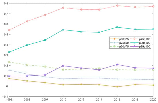
Figure 1.
The time trend of the quartile of wealth. Data source: Authors’ calculation based on CHIP and CFPS data.
Based on the previous findings, we adopt the methodology of Li and Wan (2015) [7] and Costa and Perez-Duarte (2019) [26], comparing the Lorenz curves for 1995, 2010, and 2020. The resultant outcomes are depicted in Figure 2. Notably, substantial differences emerge in the evolution of wealth distribution in China between the periods of 1995 to 2010 and 2010 to 2020. During the former period, there was a discernible trend of wealth concentration shifting from the lower strata to the upper echelons. Utilizing as a threshold, it becomes evident that the share of wealth held by groups below this threshold diminished, while that of groups above it increased. ( represents the quantile point from the bottom. For instance, denotes the bottom 10% quantile of the wealth distribution. Additionally, – represents the stratum calculated from the bottom, ranging from the wealth distribution i to j.) Conversely, from 2010 to 2020, a repositioning of wealth occurred within both the bottom 94% and top 6% segments. Specifically, the share of wealth held by the bottom 67% group shifted towards the – group, which primarily contributed to the widening wealth gap during this period. Simultaneously, there was an internal transfer of wealth within the top 6% group whereby resources previously concentrated among only those belonging to the topmost percentile were distributed across individuals falling within the – range instead. This redistribution improved the overall wealth inequality and mitigated its deterioration to some extent. On the other hand, in terms of the magnitude of wealth transfer, a substantial wealth shift occurred between 1995 and 2010, resulting in a total transfer of 22.5 percentage points from the bottom 84% to the top 16%. Consequently, both the Gini coefficient of wealth and various generalized entropy indexes experienced significant increases during this period. However, in the subsequent stage, the scale of wealth transfer was restricted to less than 2.5 percentage points, exerting offsetting effects and leading to only marginal changes in various inequality indicators from 2010 to 2020.
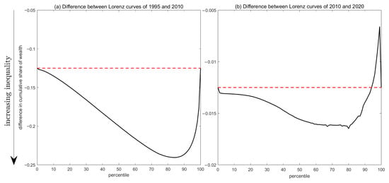
Figure 2.
The differences of Lorenz curves. Note: The red dashed line represents the baseline with a change equal to 0, while the black solid line represents the real Loernz curve change. The vertical axis represents the disparity in cumulative wealth shares, and a smaller curve value indicates a higher level of wealth inequality.
5. Reasons for the Evolution of Wealth Inequality
According to our findings in Section 4, the evolution of wealth inequality in China can be categorized into two distinct stages: first, a period of rapid escalation from 1995 to 2010 and, second, a subsequent phase characterized by the stabilization of wealth inequality from 2010 to 2020. In order to investigate the underlying causes driving this evolution, we initially conducted an analysis on the impact exerted by various asset types. Furthermore, we assessed how urban and rural communities and coastal and inland regions influenced the overall wealth disparity.
5.1. Wealth Inequality Decomposition by Components
According to the rules proposed by Lerman and Yitzhaki (1985) [27], we can elucidate the role of different assets in shaping the Gini coefficient through a comprehensive decomposition of wealth, as follows:
where represents the asset share of the k-th class. and represent the mean value and net wealth of the k-th class of assets, respectively. Additionally, represents pseudo-Gini. (The Pseudo-Gini measure differs from the Gini coefficient in its calculation methodology. Specifically, while the Gini coefficient is computed by sorting in ascending order, the pseudo-Gini measure relies on arranging in ascending order). The variable represents the correlation between the Gini coefficient of the k-th asset class and net wealth, whereas represents the Gini coefficient of the k-th asset class.
The contribution of the k-th asset class to the Gini coefficient follows Equation (2),
and the marginal contribution of the k-th asset class to the Gini coefficient follows Equation (3),
Table 7 presents the calculation results of Gini coefficients for various asset types. The findings indicate that the Gini coefficient of land has consistently increased over the study period, while the other five asset types exhibit a phased change in line with previous research. (The increase in the land Gini coefficient can be easily comprehended. With China’s economy experiencing rapid development, there has been a stable and enduring transformation of its industrial structure, leading to a gradual shift of rural labor forces from agriculture to manufacturing and service sectors. This phenomenon elucidates the continuous rise in China’s land Gini coefficient prior to 2014. In 2014 and 2016, China introduced legislations on separating land ownership, contracting rights, and management rights (Opinions on the Pilot Work of Reforming Rural Land Expropriation, Collective Operating Construction Land Marketization and Homestead System) of rural land. These measures facilitated land transfers, which further contributed to the concentration of land holdings, thereby perpetuating an upward trend in the land Gini coefficient.) Net housing, durable goods, financial assets, and productive fixed assets all experienced an increase between 1995 and 2010 but slightly decreased from 2010 to 2020. Notably, non-housing debts demonstrate a U-shaped pattern. However, given its negative impact on net wealth, this trend aligns with the other four asset types.
Table 7.
Gini coefficients for different assets in China.
The contributions of various assets to the Gini coefficient of wealth are presented in Table 8. It is evident from the table that net housing assets exert the most significant influence on wealth inequality in China, with an impact ranging from 44% to 80%, and exhibit phased characteristics consistent with changes in total wealth inequality. The contribution of land assets gradually diminishes over time, accounting for 25.5% in 1995 and only 0.9% in 2020. (The negative Gini correlation coefficient between land assets and total assets resulted in a negative contribution of land assets in 2008. A straightforward economic explanation for this result is with the development of Chinese cities. More and more rural people are entering urban areas. Individuals who stay in rural areas to cultivate are relatively poor, but they have more land assets. The correlation between ownership of land assets and personal wealth is negative, and land assets actually reduce the wealth Gini coefficient). This is mainly because China’s land system stipulates that rural land is given to collective ownership, and farmers only have the right to contract land with a long term. (The contract duration was set at 15 years in 1984 and extended to 30 years in the second round of contracts. For details, please refer to “Notice on Rural Work in 1984” and “Notice on the Issuance and Implementation of Several Policy Measures for the Current Development of Agriculture and the Rural Economy”. Additionally, the 19th National Congress of the Communist Party of China further stipulated that, upon the expiration of the current contract term, it will be extended for an additional 30 years). This long-term contracting system limits capital investment in agriculture, keeping it dominated by small-scale farming. Consequently, the lack of corresponding market-oriented reforms has made agriculture develop more slowly than the manufacturing and service sectors, resulting in a declining economic share. This shift leads to a smaller portion of income from agriculture, reflecting in a lower share of land value in household wealth and a weaker impact on the Gini coefficient. After the “three rights separation system” reform mentioned above, the restrictions on land use rights have been relaxed, leading to an increase in the contribution of land assets from 2010 to 2012. However, the current situation of China’s small-scale agricultural economy has not completely changed, and the proportion of agricultural income to economic income is still relatively low.
Table 8.
Contributions of different assets for the Gini coefficient in China (%).
Durable goods and financial assets display a U-shaped pattern regarding their impact on wealth inequality, ranging from 3% to 10% and from 6% to 28%, respectively. Productive fixed assets do not exhibit any distinct characteristics, with an impact range of 2% to 12%. In contrast, non-housing debts have consistently maintained a negligible impact on wealth inequality below the 1% level.
We posit that the predominant role of net housing assets in the Gini coefficient of per capita net wealth can be attributed to two key factors. First, during the period from 1995 to 2010, the housing market in China underwent significant transformations as a result of market-oriented reforms. In particular, in 1998, China terminated its welfare-based housing allocation system and officially introduced a monetized housing allocation system. With the initiation of personal housing mortgage loans in the same year, China entered the era of commercial housing. This market-oriented reform exerted sustained upward pressure on the concentration of housing assets. Second, there was a substantial increase in the proportion of net housing assets within net wealth, rising from 34.6% in 1995 to over 70% after 2010, more than doubling its share. These dual reasons collectively play a pivotal role in shaping the evolution of per capita net wealth’s Gini coefficient. The Appendix B presents analogous decomposition analysis for Theil index of per capita net wealth and yields results akin to those obtained for the Gini coefficient. (The decline in the net housing assets’ Gini coefficient and the significance of net housing to wealth inequality since 2010 can be attributed to the Chinese government’s recognition of the substantial wealth gap caused by soaring housing prices and the subsequent implementation of regulatory measures, thereby mitigating the contribution of net housing to China’s wealth disparity. Notably, with the issuance of the “Notice of the State Council on Resolutely Curbing Excessive Housing Price Increases in Select Cities” after 2010, China entered an era characterized by real estate regulation). We have also decomposed the marginal contributions of various assets to the Gini coefficient based on Equation (3), and the results are shown in the Appendix B.
We further examine the contributions of different assets to alterations in the Gini coefficient. According to Paul et al. (2017) [28] and Kanbur et al. (2021) [6], the changes in the Gini coefficient of per capita net wealth can be decomposed as the following Equation (4):
where represents the absolute contribution of asset k-th class to the Gini coefficient of wealth in period t. According to the formula, the change in the Gini coefficient of wealth can be decomposed into a weighted sum of the absolute contributions of different assets to the Gini coefficient, where the weight represents each asset category’s contribution to the overall Gini coefficient of wealth. The results of the decomposition analysis on the change in the Gini coefficient of wealth are presented in Table 9.
Table 9.
Decomposition of Gini coefficient change in China (%).
The table reveals several key findings: First, in line with prior research, China experienced a significant increase in its wealth Gini coefficient between 1995 and 2010 and remained relatively stable during the period from 2010 to 2020. Second, net housing assets were identified as the primary driver behind the surge in wealth inequality between 1995 and 2010, explaining 82.79% of the observed change. Productive fixed assets also played a significant role, accounting for approximately 6.24% of the change. The increase in the Gini coefficient during this period was partially offset by land and financial assets, resulting in respective decreases of 22.04% and 6.52%. Durable goods and non-housing assets had a negligible impact on the Gini coefficient. However, from 2010 to 2020, the influence of net housing and land diminished, while financial assets emerged as the dominant factor, contributing to an 8.14% increase in the Gini coefficient. This shift primarily drove the overall rise in inequality during this period. In summary, there exists a strong substitution relationship between net housing and financial assets. Initially, rising housing prices led Chinese residents to shift wealth from financial assets to real estate; subsequently, government regulations on the property market prompted a redirection of wealth from housing back to financial assets. (In December 2016, the Central Economic Work Conference proposed promoting the steady and healthy development of the real estate market, emphasizing the principle that “houses are for living in, not for speculation.” The Central Economic Work Conferences in 2017, 2018, and 2019 also repeatedly stressed the importance of real estate market control policies to ensure the market’s steady and healthy development.) Additionally, China has implemented various policies to reform the capital market and promote its high-quality development. This provides policy support for households to transfer their wealth from housing to financial assets. For example, in 2017, China harmonized the IPO standards, audit content, and procedures between the main board and the ChiNext board, facilitating the marketization of IPOs and pricing. Additionally, the implementation of the registration system in 2019 has improved IPO efficiency and encouraged the further transfer of household wealth to financial assets. Similar patterns can also be observed in the Appendix B regarding changes in Theil Index deconstruction results.
5.2. Wealth Inequality Decomposition by Subgroups
Another perspective to understand the changes in wealth inequality in China is to decompose by population subgroups. According to Young (2013) [29] and Wang et al. [30], urban–rural inequality plays an important role in China’s income and wealth distribution. Meanwhile, Kanbur et al. (2021) [6] shows that there is a large economic gap between the eastern coastal areas and the inland areas, which also has an important impact on China’s wealth disparity. In order to understand the impact of components on China’s wealth inequality, we apply the decomposition method proposed by Dagum (1998) [31] to disaggregate the Gini coefficient of wealth into within-group and between-group components, as the following Equation (5):
where indicates the Gini coefficient of subgroup i, indicates an extended Gini ratio between subgroup j and subgroup j. and represents the population share and wealth share of subgroup i, respectively.
The results in Table 10 reveal that the Gini coefficients of rural areas, as well as the extended Gini coefficient between urban and rural areas, exhibited phased changes consistent with the overall Gini coefficient. From 1995 to 2010, these coefficients experienced significant increases. However, from 2010 to 2020, the increase in the Gini coefficient was relatively small. The change in the urban Gini coefficient is strange; it decreased from 1995 to 2008 but slightly increased from 2008 to 2020. In terms of their contributions, it was observed that urban areas’ contribution to wealth inequality measured by the Gini coefficient increased from 10.37% in 1995 to 44.6% in 2020. Conversely, rural areas’ contribution continuously decreased from 44.03% in 1995 to merely 7.13% in 2020. This trend can be attributed to the expanding population share and asset distribution within urban areas, which further exacerbated the wealth gap, as depicted in Figure 3. Between-group inequality exhibits an inverted U-shaped pattern, reaching its peak at 63.77% in 2008, and its contribution rate remained between 45% and 64% during the entire period.
Table 10.
Decomposition of the Gini coefficient by urban and rural groups.
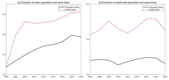
Figure 3.
Evolution of population and asset share for urban and coastal areas.
Considering the economic development disparity between coastal and inland provinces in China since the initiation of reform and opening up, we have employed Equation (5) to decompose the wealth Gini coefficient from the perspective of coastal and inland provinces. The outcomes are presented in Table 11. It is evident from the table that both the wealth Gini coefficient and the extended Gini coefficient of coastal and inland provinces exhibit stage changes consistent with the overall Gini coefficient. However, regarding their contributions, there has been minimal alteration in inequality among coastal, inland, and group divisions compared with rural–urban decomposition. These three categories fluctuate around the levels of 21%, 25%, and 53%. This discrepancy arises due to a lack of sustained growth in population share and asset share within coastal regions. As shown in Figure 3, the former remains relatively stable at approximately 38%, while the latter varies within the range of 50–60%.
Table 11.
Decomposition of the Gini coefficient by coastal and inland groups.
6. Conclusions
Since the reform and opening up, China’s economy has developed rapidly. Accompanying this economic growth is a significant rise in household income and wealth. However, the impact of rapid economic growth is uneven, and there has been a marked deterioration in the distribution of household wealth. This article utilizes CHIP micro-survey data from 1995 to 2008 and CFPS micro-survey data from 2010 to 2020 to investigate the evolution of wealth inequality in China and analyze the factors contributing to changes in wealth distribution.
First, our article argues that the evolution pattern of wealth inequality in China, as delineated by our constructed indicators (wealth Gini coefficient and generalized entropy index) based on micro survey data, can be divided into two stages. From 1995 to 2010, China’s wealth inequality increased rapidly, but from 2010 to 2020, it tended to ease.
Second, by decomposing the wealth inequality indicators based on the components, we find that changes in net housing assets are the main cause of the rise in China’s wealth gap from 1995 to 2010, with land assets exerting a mitigating effect during this period. From 2010 to 2020, with the reform of the real estate market, financial assets increasingly played a significant role in shaping disparities in wealth distribution.
Finally, we further decompose the wealth gap indicators by subgroups. The results of the rural–urban decomposition show that the impact of intra-urban inequality gradually increases, while the impact of intra-rural inequality decreases. This is mainly because the rural population is gradually moving to the cities, and the asset share of the cities is also gradually increasing, which makes the impact of intra-urban inequality increasingly important. The impact of the disparity between urban and rural areas exhibits an inverted U-shaped pattern. The coastal–inland decomposition results show that the disparity within both coastal and inland regions, as well as between these subgroups, remains relatively stable. Overall, disparities within urban areas, between urban and rural areas, and between inland and coastal regions have significant implications.
While this study enhances our understanding of China’s wealth inequality and seeks to explain its dynamic evolution, it has limitations that warrant further research. First, we must acknowledge that although we have made considerable efforts to enhance data comparability, the differences in data sources may still have some impact on the results especially in terms of viewing 2010 as the transition point. What is more, although our findings suggest that urbanization processes and policies regarding the real estate market and land institutions can significantly impact wealth inequality, we do not quantify their level. At the same time, China experienced rapid economic expansion and an increase in wealth disparities from 1995 to 2010. However, economic growth decelerated from 2010 to 2020. (Nevertheless, the GDP growth rate remained high in this period. From 2010 to 2019, China consistently achieved GDP growth rates exceeding 6%. However, due to the pandemic, the GDP growth rate in 2020 was only 2.2%). During this period, the wealth inequality in China remained relatively stable. Therefore, what is the internal relationship between China’s economic growth and the evolution of wealth distribution? This needs to be studied further.
Author Contributions
Conceptualization, Z.Z., S.L. and F.L.; methodology, Z.Z. and S.L.; software, Z.Z. and S.L.; validation, Z.Z., S.L. and F.L.; formal analysis, Z.Z. and S.L.; investigation, Z.Z. and S.L.; resources, F.L.; data curation, Z.Z. and S.L.; writing—original draft preparation, Z.Z. and S.L.; visualization, Z.Z.; supervision, F.L.; project administration, F.L.; funding acquisition, F.L. All authors have read and agreed to the published version of the manuscript.
Funding
This research was funded by the major project of the Humanities and Social Sciences Base of the Ministry of Education of China, Study on the Origins of Chinese Economics and the Construction of Autonomous Knowledge System (23JJD790012).
Institutional Review Board Statement
Not applicable.
Informed Consent Statement
Not applicable.
Data Availability Statement
The data are available upon request from the authors.
Conflicts of Interest
The authors declare no conflicts of interest.
Appendix A. The Definition and Measurement Methods of Various Types of Assets
Below we explain in detail how each type of asset is defined and measured. In Section 3, we divided household wealth into six components. Here, we will go through the definition and measurement of each asset in detail.
Land assets: China’s land institution indicates that the ownership of land belongs to the state, and farmers only have the right to use the land. Therefore, whether to include land in household wealth is a controversial issue. However, considering that the benefits of land belong to farmers, it is difficult to reflect the real wealth distribution without including land in wealth. Moreover, the individual’s right to use land is relatively stable. Therefore, following research by Li and Wan (2015) [7] and Piketty et al. (2019) [1], we include land in our wealth calculations. The CFPS data provide land values and calculation methods. Referring to McKinley and Griffin (1993) [32], they assume that 25% of the total agricultural income is derived from land with a land yield rate of 8% calculated as , where and represent the value of land asset and the total agricultural income for household i at time t, respectively. CHIP data do not provide land values, but do provide the total agricultural income. Therefore, we calculated the value of land owned by households from 1995 to 2008 using the aforementioned formula.
Net housing: CHIP and CFPS data provide housing values. According to their questionnaires, housing values are mainly derived from estimates by the interviewees. CFPS data have adjusted housing values based on surrounding house prices and house size to avoid errors in individual estimates. The CHIP data have not provided instructions for similar adjustments. In our calculations, the net housing assets equal housing values minus the housing debts. Additionally, CHIP 2008 did not provide statistics on housing debts for rural households; we used the Random Forest algorithm to interpolate the missing values as described in the text.
Durable goods: Durable goods are the value of durable consumer goods, which include cars, televisions, computers, refrigerators. and other common household consumer goods. For some years, data on durable goods are missing, but we have supplemented them as described in the main text.
Financial assets: Financial assets include deposits, stocks, funds, bonds, financial derivatives, other financial products, and money lent to other people.
Productive fixed assets: Productive fixed assets include business assets, agricultural machinery, and other similar items.
Non-housing debts: Non-housing debts are loans to both financial and non-financial institutions. Note that the values are positive.
Appendix B
The model is decomposed by employing the following (A1):
where represents the Theil Index of the group, and is the Theil Index calculated with the mean value of each group as the element and the number of each group as the weight.
Table A1.
Share of various assets in total net wealth in China (%).
Table A1.
Share of various assets in total net wealth in China (%).
| Year | Land | Net Housing | Durable Goods | Financial Assets | Productive Fixed Assets | Non-Housing Debts |
|---|---|---|---|---|---|---|
| 1995 | 34.40 | 34.62 | 10.59 | 16.62 | 4.47 | −0.69 |
| 2002 | 16.69 | 51.25 | 6.30 | 22.67 | 4.32 | −1.24 |
| 2008 | 10.33 | 68.61 | 4.18 | 13.67 | 4.21 | −1.00 |
| 2010 | 7.50 | 77.06 | 6.57 | 6.75 | 4.70 | −2.59 |
| 2012 | 7.49 | 71.64 | 5.60 | 10.55 | 8.59 | −3.88 |
| 2014 | 5.49 | 76.80 | 5.90 | 10.85 | 4.02 | −3.06 |
| 2016 | 4.67 | 72.62 | 7.29 | 12.59 | 5.49 | −2.66 |
| 2018 | 2.36 | 78.35 | 6.11 | 10.70 | 4.54 | −2.07 |
| 2020 | 2.85 | 71.78 | 7.81 | 15.40 | 4.51 | −2.35 |
Data source: Authors’ calculation based on CHIP and CFPS data.
Table A2.
The quartile wealth share in China (%).
Table A2.
The quartile wealth share in China (%).
| Year | p00p10 | p10p20 | p20p30 | p30p40 | p40p50 | p50p60 | p60p70 | p70p80 | p80p90 | p90p100 |
|---|---|---|---|---|---|---|---|---|---|---|
| 1995 | 1.45 | 3.56 | 4.82 | 5.89 | 6.94 | 8.13 | 9.59 | 11.62 | 15.14 | 32.85 |
| 2002 | 0.85 | 2.57 | 3.52 | 4.44 | 5.45 | 6.74 | 8.58 | 11.40 | 16.85 | 39.60 |
| 2008 | 0.53 | 1.70 | 2.49 | 3.32 | 4.36 | 5.86 | 7.98 | 11.32 | 18.04 | 44.39 |
| 2010 | −0.30 | 0.89 | 1.68 | 2.55 | 3.59 | 4.89 | 6.70 | 9.79 | 15.73 | 54.48 |
| 2012 | −0.25 | 1.11 | 1.92 | 2.80 | 3.82 | 5.10 | 6.98 | 9.99 | 15.96 | 52.56 |
| 2014 | −0.49 | 1.01 | 1.87 | 2.81 | 3.91 | 5.30 | 7.15 | 10.19 | 16.32 | 51.94 |
| 2016 | −2.33 | 0.91 | 1.67 | 2.51 | 3.56 | 4.90 | 6.69 | 9.66 | 15.51 | 56.92 |
| 2018 | −0.11 | 0.92 | 1.59 | 2.39 | 3.31 | 4.66 | 6.65 | 9.71 | 16.07 | 54.82 |
| 2020 | −0.56 | 0.81 | 1.47 | 2.24 | 3.27 | 4.75 | 6.67 | 9.81 | 16.57 | 54.98 |
Note: represents the stratum calculated from the bottom, ranging from the wealth distribution i to j. For instance, p10–p20 denotes the stratum situated between the bottom 10% and 20% of the wealth distribution. Data Source: Authors’ calculation based on CHIP and CFPS data.
Table A3.
The per capita net wealth inequality in China without CPI adjustment.
Table A3.
The per capita net wealth inequality in China without CPI adjustment.
| Year | Data | Gini | |||
|---|---|---|---|---|---|
| 1995 | CHIP | 0.4228 | 0.3139 | 0.3666 | 1.1250 |
| 2002 | CHIP | 0.5206 | 0.4626 | 0.5037 | 0.9929 |
| 2008 | CHIP | 0.5827 | 0.6320 | 0.6280 | 1.1739 |
| 2010 | CFPS | 0.6740 | 0.9404 | 0.9631 | 3.4157 |
| 2012 | CFPS | 0.6539 | 0.8331 | 0.8687 | 2.4113 |
| 2014 | CFPS | 0.6548 | 0.8419 | 0.8257 | 2.0073 |
| 2016 | CFPS | 0.7204 | 0.9389 | 1.0211 | 4.9873 |
| 2018 | CFPS | 0.6794 | 0.9289 | 0.9504 | 2.7502 |
| 2020 | CFPS | 0.6891 | 0.9672 | 0.9349 | 2.4467 |
Data source: Authors’ calculation based on CHIP and CFPS data.
Table A4.
Marginal contributions of various assets to the Gini coefficient of wealth in China (%).
Table A4.
Marginal contributions of various assets to the Gini coefficient of wealth in China (%).
| Year | Land | Net Housing | Durable Goods | Financial Assets | Productive Fixed Assets | Non-Housing Debts |
|---|---|---|---|---|---|---|
| 1995 | −8.90 | 9.48 | −1.13 | 0.36 | −0.54 | 0.73 |
| 2002 | −12.98 | 8.86 | −0.63 | 4.73 | −1.56 | 1.59 |
| 2008 | −10.42 | 9.70 | −0.40 | −0.33 | 0.09 | 1.35 |
| 2010 | −5.34 | 2.15 | −0.85 | −0.22 | 1.65 | 2.63 |
| 2012 | −4.79 | −0.18 | −0.99 | −0.77 | 2.56 | 4.17 |
| 2014 | −3.80 | 2.16 | −1.54 | −0.42 | −0.24 | 3.84 |
| 2016 | −2.99 | 2.95 | −1.77 | −1.31 | 0.09 | 3.03 |
| 2018 | −1.87 | 1.53 | −1.36 | −0.88 | 0.68 | 1.90 |
| 2020 | −1.91 | 1.93 | −1.79 | −1.02 | 0.38 | 2.42 |
Data source: Authors’ calculation based on CHIP and CFPS data.
Table A5.
Contributions of different assets for the coefficient in China (%).
Table A5.
Contributions of different assets for the coefficient in China (%).
| Year | Land | Net Housing | Durable Goods | Financial Assets | Productive Fixed Assets | Non-Housing Debts |
|---|---|---|---|---|---|---|
| 1995 | 12.31 | 48.05 | 20.38 | 16.53 | 2.38 | 0.34 |
| 2002 | −8.87 | 66.01 | 5.38 | 35.37 | 1.29 | 0.82 |
| 2008 | −10.79 | 88.05 | 3.29 | 13.24 | 5.75 | 0.45 |
| 2010 | −3.79 | 79.27 | 4.33 | 6.49 | 13.01 | 0.69 |
| 2012 | −2.52 | 69.40 | 3.06 | 8.61 | 20.78 | 0.67 |
| 2014 | −2.68 | 85.31 | 2.39 | 10.41 | 3.45 | 1.12 |
| 2016 | −1.41 | 81.21 | 2.75 | 9.86 | 6.81 | 0.78 |
| 2018 | −1.53 | 82.79 | 2.37 | 7.87 | 8.01 | 0.49 |
| 2020 | −1.26 | 77.54 | 3.67 | 13.42 | 5.97 | 0.66 |
Data source: Authors’ calculation based on CHIP and CFPS data.
Table A6.
Decomposition of change in China for various asstes (%).
Table A6.
Decomposition of change in China for various asstes (%).
| Year | Changes in the Gini Coefficient | Land | Net Housing | Durable Goods | Financial Assets | Productive Fixed Assets | Non-Housing Debts |
|---|---|---|---|---|---|---|---|
| 1995–2002 | 33.87 | −24.18 | 40.32 | −13.18 | 30.82 | −0.65 | 0.75 |
| 2002–2008 | 29.49 | −5.11 | 48.01 | −1.12 | −18.22 | 6.16 | 0.23 |
| 2008–2010 | 52.36 | 5.03 | 32.72 | 3.31 | −3.35 | 14.07 | 0.59 |
| 2010–2012 | −9.43 | 1.51 | −16.41 | −1.56 | 1.30 | 5.81 | −0.08 |
| 2012–2014 | −5.50 | −0.02 | 11.22 | −0.80 | 1.23 | −17.52 | 0.39 |
| 2014–2016 | 22.93 | 0.95 | 14.52 | 0.99 | 1.71 | 4.92 | −0.16 |
| 2016–2018 | −7.04 | −0.01 | −4.24 | −0.55 | −2.55 | 0.64 | −0.33 |
| 2018–2020 | −0.89 | 0.28 | −5.95 | 1.27 | 5.43 | −2.09 | 0.17 |
| 1995–2010 | 164.12 | −22.31 | 161.31 | −8.94 | 0.61 | 31.97 | 1.46 |
| 2010–2020 | −3.05 | 2.56 | −4.10 | −0.77 | 6.51 | −7.22 | −0.05 |
| 1995–2020 | 156.05 | −15.53 | 150.49 | −10.99 | 17.82 | 12.92 | 1.34 |
Data source: Authors’ calculation based on CHIP and CFPS data.
Table A7.
Decomposition of the coefficient by urban and rural groups.
Table A7.
Decomposition of the coefficient by urban and rural groups.
| Year | Within-Group (Urban/Rural) Inequality | Between-Group Inequality | ||||
|---|---|---|---|---|---|---|
| of Urban Areas | Contribution (%) | of Rural Areas | Contribution (%) | between Urban and Rural | Contribution (%) | |
| 1995 | 0.5578 | 43.08 | 0.2898 | 56.67 | 0.0009 | 0.24 |
| 2002 | 0.4105 | 49.20 | 0.2787 | 23.39 | 0.1345 | 27.41 |
| 2008 | 0.4056 | 46.49 | 0.3920 | 16.76 | 0.3675 | 36.61 |
| 2010 | 0.8529 | 62.40 | 0.7476 | 22.53 | 0.1460 | 15.08 |
| 2012 | 0.7797 | 63.99 | 0.7139 | 22.85 | 0.1154 | 13.16 |
| 2014 | 0.7629 | 66.57 | 0.6214 | 20.39 | 0.1086 | 13.04 |
| 2016 | 0.9423 | 70.92 | 0.7353 | 18.14 | 0.1094 | 10.93 |
| 2018 | 0.7909 | 68.00 | 1.0455 | 20.42 | 0.1098 | 11.58 |
| 2020 | 0.8307 | 72.06 | 0.7201 | 14.20 | 0.1290 | 13.73 |
Data source: Authors’ calculation based on CHIP and CFPS data.
Table A8.
Decomposition of the coefficient by coastal and inland groups.
Table A8.
Decomposition of the coefficient by coastal and inland groups.
| Year | Within-Group (Coastal/Inland) Inequality | Between-Group Inequality | ||||
|---|---|---|---|---|---|---|
| of Coastal Areas | Contribution (%) | of Inland Areas | Contribution (%) | between Coastal and Inland | Contribution (%) | |
| 1995 | 0.3549 | 51.03 | 0.2884 | 37.21 | 0.0431 | 11.76 |
| 2002 | 0.4864 | 54.59 | 0.3753 | 34.36 | 0.0542 | 11.05 |
| 2008 | 0.5845 | 55.45 | 0.4627 | 28.92 | 0.0993 | 15.63 |
| 2010 | 0.9574 | 55.11 | 0.7906 | 36.15 | 0.0846 | 8.74 |
| 2012 | 0.9179 | 55.92 | 0.7171 | 38.10 | 0.0525 | 5.99 |
| 2014 | 0.8676 | 59.50 | 0.6264 | 32.63 | 0.0652 | 7.87 |
| 2016 | 1.0440 | 61.92 | 0.7650 | 29.72 | 0.0852 | 8.36 |
| 2018 | 0.9029 | 58.69 | 0.7670 | 31.13 | 0.0964 | 10.18 |
| 2020 | 0.9894 | 57.96 | 0.7200 | 34.53 | 0.0705 | 7.51 |
Data source: Authors’ calculation based on CHIP and CFPS data.
References
- Piketty, T.; Yang, L.; Zucman, G. Capital accumulation, private property, and rising inequality in China, 1978–2015. Am. Econ. Rev. 2019, 109, 2469–2496. [Google Scholar] [CrossRef]
- Knight, J.B.; Li, S.; Wan, H. The Increasing Inequality of Wealth in China, 2002–2013; Technical report; CHCP Working Paper: Houston, TX, USA, 2017. [Google Scholar]
- Cai, H.; Chen, Y.; Zhou, L. Income and Consumption Inequality in Urban China: 1992–2003. Econ. Dev. Cult. Chang. 2010, 58, 385–413. [Google Scholar] [CrossRef]
- Xie, Y.; Zhou, X. Income inequality in today’s China. Proc. Natl. Acad. Sci. USA 2014, 111, 6928–6933. [Google Scholar] [CrossRef]
- Wang, C.; Wan, G.; Yang, D. Income Inequality in the People’s Republic of China: Trends, Determinants, and Proposed Remedies. In China’s Economy; John Wiley and Sons, Ltd.: Hoboken, NJ, USA, 2015; Chapter 7; pp. 99–123. [Google Scholar]
- Kanbur, R.; Wang, Y.; Zhang, X. The great Chinese inequality turnaround. J. Comp. Econ. 2021, 49, 467–482. [Google Scholar] [CrossRef]
- Li, S.; Wan, H. Evolution of wealth inequality in China. China Econ. J. 2015, 8, 264–287. [Google Scholar] [CrossRef]
- Wu, Y.B.; Zhang, W. Housing ownership and housing wealth: New evidence in transitional China. Hous. Stud. 2019, 34, 448–468. [Google Scholar] [CrossRef]
- Cheng, Z.; Prakash, K.; Smyth, R.; Wang, H. Housing wealth and happiness in Urban China. Cities 2020, 96, 102470. [Google Scholar] [CrossRef]
- Zhang, P.; Sun, L.; Zhang, C. Understanding the role of homeownership in wealth inequality: Evidence from urban China (1995–2018). China Econ. Rev. 2021, 69, 101657. [Google Scholar] [CrossRef]
- Wan, H.; Knight, J. China’s growing but slowing inequality of household wealth, 2013–2018: A challenge to ‘common prosperity’? China Econ. Rev. 2023, 79, 101947. [Google Scholar] [CrossRef]
- Zucman, G. Global wealth inequality. Annu. Rev. Econ. 2019, 11, 109–138. [Google Scholar] [CrossRef]
- Piketty, T. Capital in the Twenty-First Century; Harvard University Press: Cambridge, MA, USA, 2014. [Google Scholar]
- Luo, C.; Li, S.; Sicular, T. The long-term evolution of national income inequality and rural poverty in China. China Econ. Rev. 2020, 62, 101465. [Google Scholar] [CrossRef]
- Knight, J.; Shi, L.; Haiyuan, W. Why has China’s Inequality of Household Wealth Risen Rapidly in the Twenty-First Century? Rev. Income Wealth 2022, 68, 109–138. [Google Scholar] [CrossRef]
- Zhang, C.; Xu, Q.; Zhou, X.; Zhang, X.; Xie, Y. Are poverty rates underestimated in China? New evidence from four recent surveys. China Econ. Rev. 2014, 31, 410–425. [Google Scholar] [CrossRef]
- Khan, A.R.; Griffin, K.; Riskin, C.; Renwei, Z. Household income and its distribution in China. In Chinese Economic History Since 1949; Brill: Hong Kong, China, 2017; pp. 1054–1089. [Google Scholar]
- Geng, Y.; Liu, L.; Chen, L. Rural revitalization of China: A new framework, measurement and forecast. Socio-Econ. Plan. Sci. 2023, 89, 101696. [Google Scholar] [CrossRef]
- Guo, Y.; Liu, Y. Poverty alleviation through land assetization and its implications for rural revitalization in China. Land Use Policy 2021, 105, 105418. [Google Scholar] [CrossRef]
- Ye, J. Land Transfer and the Pursuit of Agricultural Modernization in C hina. J. Agrar. Change 2015, 15, 314–337. [Google Scholar] [CrossRef]
- Wang, Q.; Zhang, X. Three rights separation: China’s proposed rural land rights reform and four types of local trials. Land Use Policy 2017, 63, 111–121. [Google Scholar] [CrossRef]
- Fei, R.; Lin, Z.; Chunga, J. How land transfer affects agricultural land use efficiency: Evidence from China’s agricultural sector. Land Use Policy 2021, 103, 105300. [Google Scholar] [CrossRef]
- Hao, R.; Wei, Z. Fundamental causes of inland–coastal income inequality in post-reform China. Ann. Reg. Sci. 2010, 45, 181–206. [Google Scholar] [CrossRef]
- Zhang, Q.; Zou, H.F. Regional inequality in contemporary China. Ann. Econ. Financ. 2012, 13, 113–137. [Google Scholar]
- Wei, K.; Yao, S.; Liu, A. Foreign direct investment and regional inequality in China. Rev. Dev. Econ. 2009, 13, 778–791. [Google Scholar] [CrossRef]
- Costa, R.N.; Pérez-Duarte, S. Not All Inequality Measures Were Created Equal: The Measurement of Wealth Inequality, Its Decompositions, and an Application to European Household Wealth; ECB Statistics Paper: Frankfurt am Main, Germany, 2019; Number 31. [Google Scholar]
- Lerman, R.I.; Yitzhaki, S. Income inequality effects by income source: A new approach and applications to the United States. Rev. Econ. Stat. 1985, 67, 151–156. [Google Scholar] [CrossRef]
- Paul, S.; Chen, Z.; Lu, M. Contribution of household income components to the level and rise of inequality in urban China. J. Asia Pac. Econ. 2017, 22, 212–226. [Google Scholar] [CrossRef]
- Young, A. Inequality, the Urban-Rural Gap, and Migration*. Q. J. Econ. 2013, 128, 1727–1785. [Google Scholar] [CrossRef]
- Wang, Y.; Li, Y.; Huang, Y.; Yi, C.; Ren, J. Housing wealth inequality in China: An urban-rural comparison. Cities 2020, 96, 102428. [Google Scholar] [CrossRef]
- Dagum, C. A New Approach to the Decomposition of the Gini Income Inequality Ratio; Springer: Berlin/Heidelberg, Germany, 1998. [Google Scholar]
- McKinley, T.; Griffin, K. The distribution of land in rural China. J. Peasant. Stud. 1993, 21, 71–84. [Google Scholar] [CrossRef]
Disclaimer/Publisher’s Note: The statements, opinions and data contained in all publications are solely those of the individual author(s) and contributor(s) and not of MDPI and/or the editor(s). MDPI and/or the editor(s) disclaim responsibility for any injury to people or property resulting from any ideas, methods, instructions or products referred to in the content. |
© 2024 by the authors. Licensee MDPI, Basel, Switzerland. This article is an open access article distributed under the terms and conditions of the Creative Commons Attribution (CC BY) license (https://creativecommons.org/licenses/by/4.0/).