Analysis of Circular Price Prediction Strategy for Used Electric Vehicles

Abstract

As the car price war has intensified in China from 2023, the continuous decline in prices of new cars for both conventional fuel vehicles and electric vehicles (EVs) has led to a sharp decline in used cars. In particular, the EV market appears more vulnerable as the prime cost of battery raw materials has decreased since January 2023. And thus, a second-hand EV price prediction system is urgent. This study compares several methods for used EVs in China. We find that the random forest method and the gradient boosting regression tree (GBRT) method have good effects on predicting used EV prices in respecting price ranges. Timed EV data capture is applied to guarantee the real-time property of our prediction system. Then, we propose the concept of circular pricing, which means that the obsolete data for the priced car will be repriced according to the latest data. In this way, such a system can guide the used car dealers to adjust the price in time.

1. Introduction

The increasingly mature battery technology and the upgrading of the manufacturing industry have driven the development of EVs in China in recent years. China has made significant progress in the development of the EV market, but at the same time, it also faces increasing challenges which are derived from various aspects. Firstly, the government polices predominate the EV market. The proportion of subsidy impact is the largest, even though the proportion has gradually decreased in recent years. A previous study in 2019 predicted that the abrogation of EV subsidy schemes would lead to a sharp decline of EV market share by 42% in China, but it seems that the EV has been accelerating to substitute for internal combustion engine vehicles (ICEVs) since 2023, even if subsidies are reduced [1,2,3]. Secondly, supply chain issues like battery supply and chip shortages should not be underestimated as the production of EV batteries is heavily dependent on the raw material input like lithium, cobalt, and nickel, which have experienced price volatility [4]. Finally, the development of the automotive recycling industry has also affected the EV market. The end-of-life vehicle recycling in China is still in its germination stage and how to deal with the end-of-life EVs and waste lithium batteries is worth pondering [5,6]. However, the challenges faced by the EV market will gradually spread to the second-hand EV market and will be mixed with various other issues such as battery degradation and warranty issues caused by manufacturers’ competition and elimination. Thus, it will promote a large number of used car transitions, leading to the decline of car prices for both new and used ones. Compared to ICEVs, the popularity of EVs is on the rise. Manufacturers continuously develop new EVs at various price ranges to seek sales growth points, contributing to further price decline. So far, there is not much experience in used EV acceptance and purchase. Pricing decisions by buyers and sellers of used EVs focus on the endowment effect [7]. The low expected price of used EVs has become a stereotype for both buyers and sellers, which is due to their comprehensive consideration of fast technological updates, safety, and market environment. For new EVs, buyers value brand effect less, which led BMW i3 to great price reduction in China [8]; instead, they prefer practicality. For used ICEV buyers, practicality is most important. But for used EVs, safety is more highly prioritized. Therefore, second-hand car dealers are more inclined to sell some quasi-new EVs to ensure they can be sold quickly. An investigation predicted that the used EV market will be three times larger than the new EV market with the shrinkage of the ICEV market and the development of the EV market [9]. We believe that with the economic downturn [10] and the development of EVs in China, people will increasingly accept used EVs. Therefore, an accurate prediction for used EVs is urgent for both buyers and sellers.

2. Related Work

Traditionally, the pricing basis for used cars is the current sales price of new vehicles in the market. The depreciation of automobiles depends on many variables such as geometric depreciation, country, and real income [11,12]. A phased depreciation rate can be designed according to the service life. For example, a car that has been in use for 8 years can be given three different depreciation rates which correspond to 3–4–1 years. Furthermore, the pricing of a used car also be deduced with driving distance and a phased depreciation. However, due to significant changes in new car prices and changes in demand for cars, the price with the traditional pricing method cannot keep up with the market changes. Therefore, there is a high demand for effective and efficient methods for used car pricing.

The booming development of big data enables us to access a large amount of data on used cars which contains brand, sales prices, mileage driven, vehicle size, car model, etc. Thus, it is easy to think of using machine learning methods for pricing which refer to linear regression, K-nearest neighbor, random forest, gradient boosting trees, and decision tree [13,14,15,16,17,18,19,20]. However, there are several problems with these studies. First, the data collection is not sufficient which behaves as the analysis only for a single brand [13], fewer records of vehicles [18], and fewer input parameters [14]. Second, the accuracy of such predictions is low [21]. The reason may be that different parameters were not given to vehicles in different price ranges in the prediction. Another reason may lie in that traditionally used car price prediction models do not provide estimates of uncertain information such as national policy or the sudden price reduction by car companies, and thus may cause overfitting problems [22]. Furthermore, the price prediction for the vehicle is a regression problem that uses indexes like mean absolute error to evaluate the model [18,22,23,24]. Nonetheless, both buyer and seller need an intuitive method to understand the predicted price and thus it is more intuitive to give a fluctuation range to the predicted price and determine the accuracy of the prediction model based on this fluctuation range. Third, the used EV price prediction needs to be discriminated from that of ICEVs as the update of EV is fast, causing bankruptcy of EV manufacturers and more people joining the industry. In most of the previous studies, researchers intend to predict vehicles according to corresponding parameters with brands without considering if they are EVs or ICEVs [19,25,26]. Fourth, it lacks the necessary analysis of prediction results. A good prediction cannot only reflect the reasonable pricing of the proposed model, but it can also be a good response to the market that reports the demands of buyers and sellers. Moreover, through website research, we found that outdated used EVs are difficult to price due to a lack of sufficient data support. However, with the development of EV technology and the decrease in prices of batteries and other accessories, it is worth studying whether used cars after maintenance have cost-effectiveness. At this point, we may need a cyclic prediction method to predict outdated EVs.

In this study, we aim to propose a used EV price prediction system that can circularly and automatically update the predictive model. In this system, we adopt a web crawler technology that can, in a timely manner, extract vehicle information based on information release time. Then, a linear regression method is combined with the Dropout module to guarantee that the model can be updated based on the latest data. In this way, the dropped data can be predicted for a new price so that we can provide the latest market for both buyer and seller in time.

3. Materials and Methods

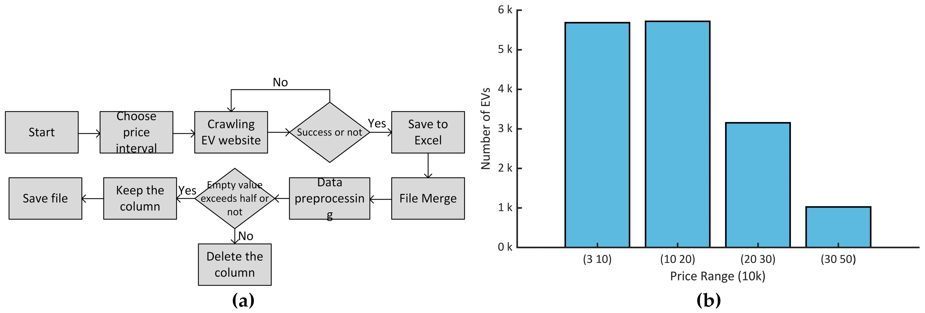
3.1. Data Collection

We utilized web scraping techniques to gather EV data from the Autohome website (https://www.autohome.com.cn/ (accessed on 3 April 2024)). Breaking down the price range into six intervals, we employed Google Chrome’s developer tools to pinpoint the hyperlink tags and EV names on each EV page. Subsequently, we crawled the relevant data using the Selenium library in Python 3.6.5, parsing hyperlink labels and car names with regular expressions, retrieve the car information through the hyperlink tags and the BeautifulSoup library 4.8.1, and storing the data in an Excel file using the Pandas library 2.2.2. This process involved crawling six times for each of the six intervals. In total, we amassed 19,476 pieces of EV information. Then, we removed unlicensed vehicles, vehicles with mileage less than 0.1 km on the odometer, vehicles with length × width × height (mm) not provided, and vehicles that were repeatedly displayed, resulting in 16,884 available data. However, we filtered out EVs such as micro-EVs and electric sports cars due to their insufficient quantity and wide price range, respectively. Consequently, we focused on data of used EVs priced between 30 to 500 thousand RMB, resulting in 15,583 pieces of EV information. Figure 1a shows the data crawling and preprocessing procedure and Figure 1b illustrates the distribution of prices.

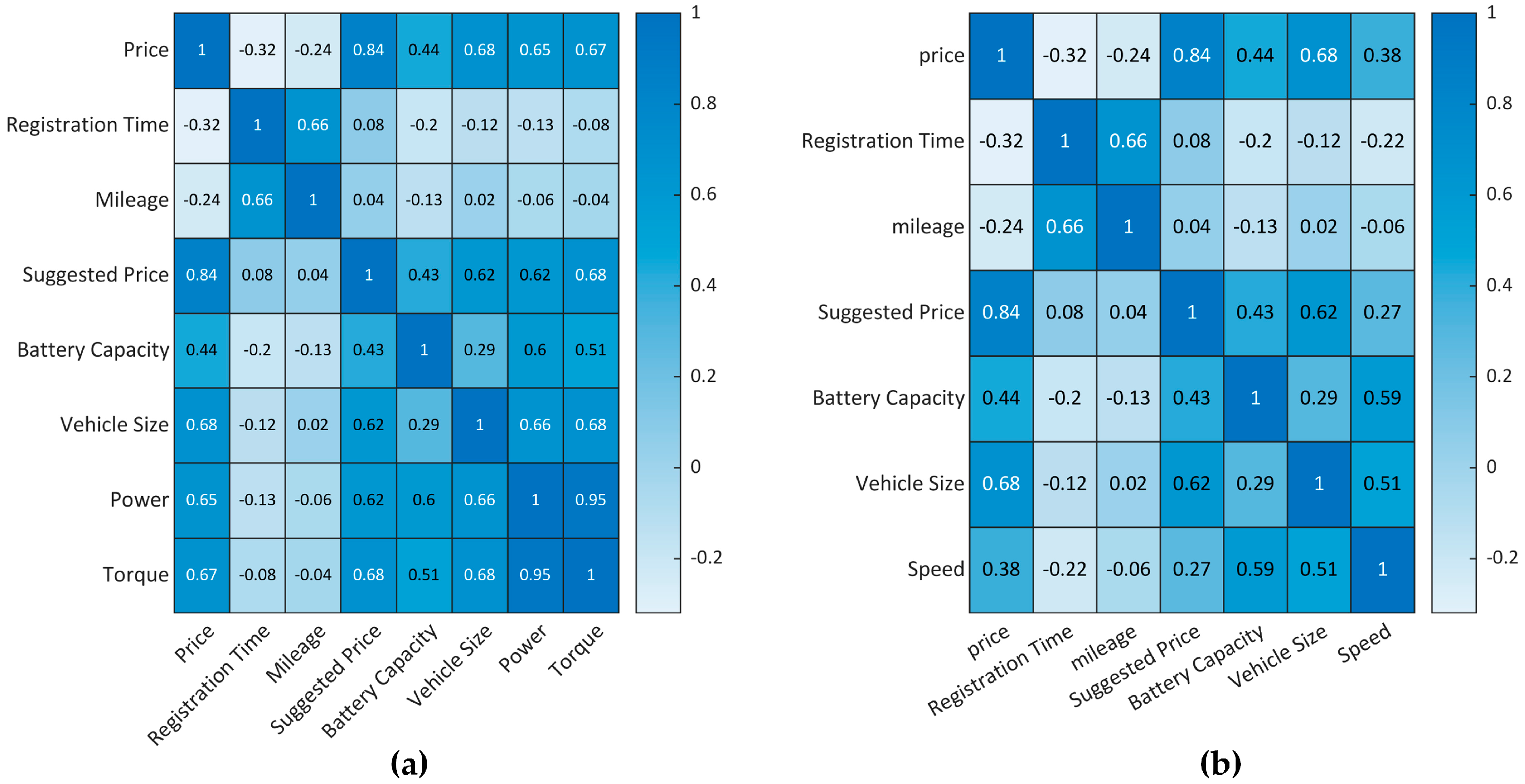
3.2. Data Processing

We utilize a combination of numerical features and texture features to predict the prices of EVs. The numerical features encompass listing price, registration time, mileage, manufacturer’s suggested price, vehicle size, maximum output power, and torque of the EV motor [27]. In Figure 2a, the suggested price, vehicle size, maximum output power, and torque of the EV motor are positively correlated with the prices of EVs. The correlation between prices and the suggested price for a new EV is as high as 0.84. The registration time, mileage, and prices are negatively correlated, which indicates that with the increase of vehicle registration time and mileage, vehicle maintenance costs rise, performance declines, and the prices of EVs tend to decrease. Finally, since the maximum output power and torque of the EV motor are highly correlated (up to 0.95), these two characteristics and price correlation are the same. To better describe the relationship between these two characteristics and prices, we instead use the speed, and the correlation between speed and prices is 0.38 (Figure 2b). The calculation for the speed is as follows:

$$T=\frac{9549\times P}{n},$$

(1)

where P is the maximum output power in kilowatts, T is the torque of the EV motor in N·m, and n is the speed in revolutions per minute (rpm). Additionally, texture features such as manufacturer, model, propulsion system, EV motor type, battery type, transmission type, and front and rear suspension type are incorporated for comprehensive analysis. These texture features undergo one-hot encoding, facilitating their integration with numerical features as inputs for various classifiers.

Normalization of all data is performed using the minimum–maximum normalization method. To ensure the robustness and accuracy of our models, we partition the data into training and testing sets, with 80% allocated for training and 20% for testing within each price range. Furthermore, we employ a five-fold cross-validation approach to validate the performance of each algorithm.

3.3. Regression Methods

The prediction accuracy of our model is an important factor for model performance evaluation. Five regression methods are adopted for comparison which are Lasso regression, regression tree, support vector regression, random forest, and GBRT model.

3.3.1. Lasso Regression

In Lasso regression, the car dataset is divided into a training set and a test set. Price is used as the target value, while attributes such as registration time, mileage, and manufacturer are used as feature values, with the corresponding feature weights initialized to 1. The regularization parameter α is set to 0.1, the learning rate is set to 0.01, and the training runs for 20,000 iterations. Gradient descent is used to minimize the objective function, updating the weights and bias until the maximum number of iterations is reached. Finally, w and b are used to predict the prices of new car data:

$$\widehat{y}=x\times w+b,$$

(2)

where $\widehat{y}$ presents the predicted price value of the car data, $x$ denotes t the feature vector of the car data, $w$ stands for the weight vector, and $b$ indicates the intercept term.

The loss value is recorded during each training iteration. The regularization parameter is adjusted by comparing the difference between the current loss value and the previous loss value. If the current loss value is greater than the previous one, the weights and intercept terms from the previous iteration are restored, and the regularization parameter is reduced to 0.1 times its original value. The loss function is denoted as

$$loss=\frac{1}{2N}{\sum }_{i=1}^N{\left({\widehat{y}}_i-y_i\right)}^2+\alpha {\sum }_{j=1}^D\left|w_i\right|,$$

(3)

where $N$ is the number of car data samples in the training set, and $D$ is the dimensionality of features. $\alpha$ is the regularization parameter, which prevents the model from overfitting.

3.3.2. Regression Tree

The regression tree is a binary recursive segmentation technique that divides the current sample into two sub-samples, ensuring that each non-leaf node has two branches [28]. The regression tree algorithm operates in two main stages: recursively splitting the samples to build the tree, followed by pruning using validation data [29].

Initially, the model consists of only the root node, which contains all the training data of the cars. Each car feature’s values are sorted, and for each car feature, the midpoint between adjacent values is calculated as a potential split point. This model searches for the best split point in the root node by iterating over all car features and potential split points, calculating the mean squared error (MSE) for each split point. For each car feature, all possible split points (denoted as t) are computed. The MSE of the left and right subtrees for each t is then calculated, using the following formula as the MSE corresponding to t:

$${MSE}_{t_{i,j}-split}=\frac{n_{t_{i,j}-left}}{N}\times {MSE}_{t_{i,j}-left}+\frac{n_{t_{i,j}-right}}{N}\times {MSE}_{t_{i,j}-right},$$

(4)

where $n_{t_{i,j}-left}$ and $n_{t_{i,j}-right}$ represent the number of samples in the left and right subtrees, respectively, and $N$ denotes the total number of car data samples at that node. $i$ indicates the $i$-th feature and $j$ represents the $j$-th potential split point. The formula to calculate the MSE for the left and right subtrees is as follows:

$$MSE=\frac{1}{n}{\sum }_{i=1}^n{\left(y_i-\widehat{y}\right)}^2,$$

(5)

where $y_i$ represents the actual price of the $i$-th sample in the subtree, $\widehat{y}$ represents the mean actual price of the samples in that subtree, and $n$ represents the number of car samples in the subtree.

After the above steps, we have obtained the regression tree model. At each node, based on the node’s splitting feature and split point, we decide whether to send the car test data to the left subtree or the right subtree. When the car test data reaches a leaf node of the car training data, the predicted price of the car test data is the average of the actual prices of all the car training data at that node.

3.3.3. Support Vector Regression

As a supervised-learning approach, SVR trains using a symmetrical loss function, which equally penalizes high and low misestimates [30]. This approach effectively presents the relationship between features and prices and can enhance the computational efficiency of SVR.

In this model, price prediction employs the Formula (2) mentioned in Lasso regression, and it is trained by inputting the features of the car data. When training the SVR model, the objective is to find the optimal $w$ and $b$, such that the error between predicted car prices and actual car prices is minimized within a certain range and also satisfying certain regularization constraints. The optimization problem can be represented as

$${min}_{w,b}\frac{1}{2}{||w||}^2+C{\sum }_{i=1}^{N}L\left(y_i,f(x_i)\right),$$

(6)

where ${||w||}^2$ is the regularization parameter (penalty coefficient), $C$ is the regularization parameter (penalty coefficient), and $L\left(y_i,f(x_i)\right)$ is the loss function, usually the $ϵ$-insensitive loss function. $N$ is the number of car data points in the training set. $y_i$ is the true value of the $i$-th car data point, and $f(x_i)$ is the predicted value of the $i$-th car data point.

The optimization problem of SVR can be solved using quadratic programming methods. Finally, through multiple experiments, the optimal parameter setting is determined, with $C$ set to 0.1, to ensure the model’s generalization ability and robustness.

3.3.4. Random Forest

Random Forest is a classic ensemble bagging algorithm that combines random sampling and multiple weak learners to train a stable and accurate model [28]. To ensure model accuracy while balancing computational time and memory consumption, we experimented with various parameters.

The Random Forest model used in the experiment is generated by extracting subsets of car data from the car training dataset. At each node split, a subset of features is randomly selected from all car features. Using this subset of car data and features, a regression tree is generated. This process is repeated to generate 200 regression trees. The method for generating the regression trees is as previously described. The difference is that in the Random Forest, each regression tree has a minimum of one sample per leaf node, the minimum number of car data samples required to split a node is set to 2, and the stopping conditions are that each node must have fewer than two samples or the depth of any node must reach 30. This parameter setting has achieved relatively good results on this dataset.

In the model, each tree predicts the price individually based on the features of the car test data. Similar to predicting prices with regression trees, when the car test data reaches a leaf node, the predicted price is the average of the prices of all car training data samples in that node. The final predicted price for the car test data is obtained by averaging the predicted prices from the 200 regression trees.

3.3.5. GBRT

In this model, each tree is optimized based on the previous one. Initially, the first tree is trained to predict prices. Subsequently, another tree is trained to predict the difference between the price predicted by the first tree and the true price. The predicted price and the difference are then added together. If discrepancies persist, further training is conducted to continuously minimize the error. The model can be expressed as [31]

$${\widehat{y}}_i=F_M\left(x\right)=F_0\left(x\right)+\eta \times \sum _{m=1}^M{h}_m\left(x\right),$$

(7)

where $F_m\left(x\right)$ represents the predicted price for the car data $x$ by the $m$-th regression tree, $F_0\left(x\right)$ is the predicted value of the first regression tree, and $\eta$ is learning rate and $h_m(x)$ represents the residual of the $m$-th regression tree for the car data $x$. For the GBRT model used in this car price prediction task, the first tree predicts car prices using the regression tree method. It sets the minimum number of samples per leaf to 1, the minimum number of car data samples required to split a node to 2, and the stopping condition to when the number of samples in each node is less than 2 or the depth of any node reaches 5. The subsequent regression trees predict prices using the following formula:

$$F_m\left(x\right)=F_{m-1}\left(x\right)+{\eta \times h}_m\left(x\right),$$

(8)

where $F_{m-1}\left(x\right)$ represents the predicted price for the car data $x$ by the previous regression tree.

The current model’s residuals are used as new target values to train a new regression tree, with the objective of minimizing the mean squared error (MSE) of these residuals. The optimization objective is formulated as follows:

$$h_m\left(x\right)=\underset{h}{\mathit{arg\; min}} L_m=\underset{h}{\mathit{arg\; min}} \sum _{i=1}^{n}l\left(y_i,F\left(x_i\right)+h\left(x_i\right)\right),$$

(9)

where $L_m$ is the loss function in the $m$-th tree, using Mean Squared Error (MSE) as the loss function.

In the training process of GBRT, we set the learning rate to 0.1 and randomly select 80% of the training samples to build the current regression tree in each iteration. To ensure that the same 80% of the samples are selected in each iteration on the same automobile dataset, we set the random seed to a fixed value (e.g., 42), thereby making the training process reproducible. After 499 iterations of prediction and residual updates, a well-trained GBRT model is obtained. Inputting the features of the automobile test data into this model, and going through iterative prediction and accumulation, yields the final predicted result.

3.4. The Evaluation Methods

We also set two criteria for predictive accuracy in which the difference between the predicted selling price and the displayed selling price shall not exceed 10% and 5%, respectively. Since predicting EV prices is a regression problem, we also evaluated our model using four different methods which are mean square error (MSE), root mean square error (RMSE), mean absolute error (MAE), and R-squared.

To evaluate the effectiveness of the numerical features and texture features, we choose classification methods that have relatively good overall performance for modeling with these two categories of features, respectively. We mainly want to distinguish the impact of these two types of feature data on classification accuracy.

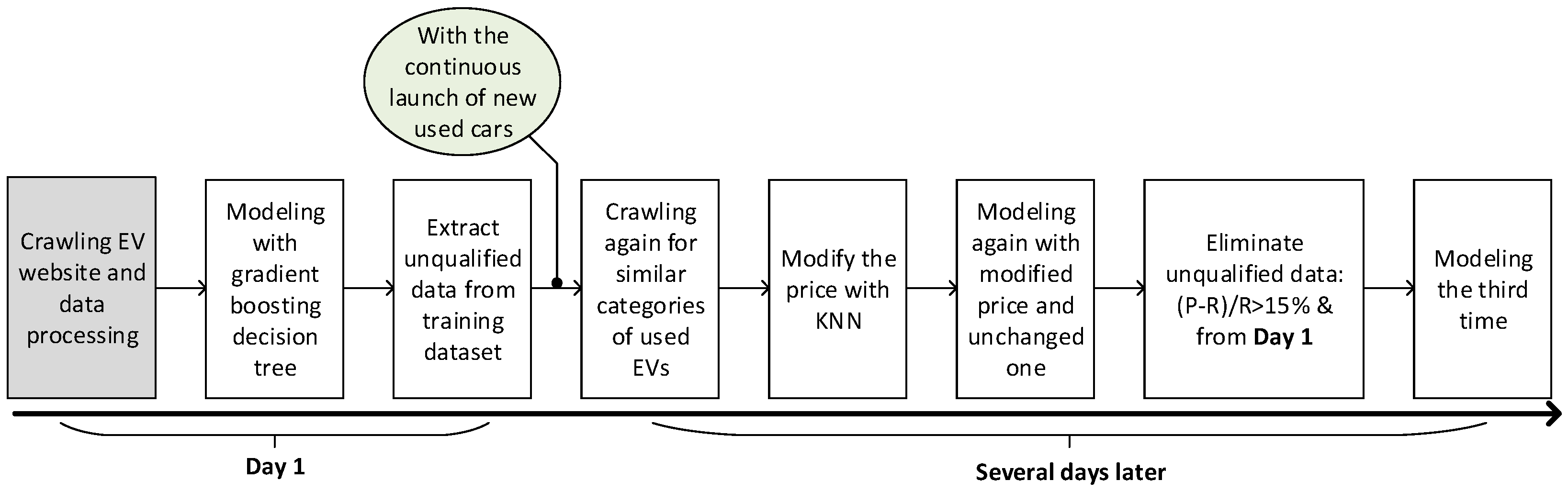
3.5. Price Updating Strategy

With the intensification of the price war for EVs, the prices of used EVs are changing faster and faster. Therefore, car owners and dealers need a reasonable method for updating the prices of used EVs.

3.5.1. Three Round Training

Here, we propose a price updating strategy that needs to perform data crawling regularly (Figure 3). First, the data crawling time is marked each time for each piece of crawled EV information, and we use the GBRT method to build a model as mentioned before, including five-fold cross-validation. Then, the training data are used as the testing one and if the predicted price exceeds 10% of the sell one, the price is selected as the unqualified one and the corresponding EV information is marked. After that, we recrawl vehicle information with the same manufacturer, body structure, vehicle class, and propulsion system as the marked EVs, and then use the KNN algorithm to predict the price of the marked EVs based on information such as registration time and mileage. Then, the unqualified price is corrected by averaging the predicted price with the GBRT method and the KNN re-predicted one for the corrected price is updated as follows:

$$y_{correction}=\frac{\left({\widehat{y}}_{GBRT}+{\widehat{y}}_{knn}\right)}{2},$$

(10)

where ${\widehat{y}}_{GBRT}$ is the predicted price from the previous round of GBRT, calculated based on feature weights, representing the predicted price of the car. ${\widehat{y}}_{knn}$ is the price of the nearest neighbor data point, indicating the latest price trend for used EVs of the same type.

Then, we build the model again with the corrected data and the unchanged one and the modeling procedure is the same as the previous one. After that, we remove the unqualified one which is crawled the first time and the unqualified one meets the requirement that the predicted price is 15% larger/smaller than the displayed price. As we have already re-crawled the data before, this unqualified data means that it has been on the website for too long and has not been sold, and it may need to be discounted. Finally, the processed data is used for modeling and model evaluation as a consequence. Training and testing numbers for each dataset are shown in

Table 1. Data sample size for price updating strategy.

	Training and Testing (1st)			Training and Testing (2nd)			Training and Testing (3rd)
Price Range	Training Dataset	Testing Dataset	Total	Training Dataset	Testing Dataset	Total	Training Dataset	Testing Dataset	Total
3–10	4548	1138	5686	6757	1690	8447	6314	1579	7893
10–20	4575	1144	5719	6188	1548	7736	5979	1495	7474
20–30	2521	631	3152	3724	931	4655	3660	916	4576
30–50	820	206	1026	1100	276	1376	1089	273	1362
3–50	12,464	3119	15,583	17,769	4445	22,214	17,042	4263	21,305

The prices need to be ×10 k.

.

3.5.2. K-Nearest Neighbor (KNN)

The KNN algorithm calculates the Euclidean distance between each prediction point and every data point in the training set, and then selects the true values of the k nearest data points based on the minimum Euclidean distance using an aggregation method to obtain the predicted value.

The manufacturer, body structure, vehicle class, propulsion system, registration time, and mileage are used as feature values for each car data point in the dataset, with the price being the target value for each car data point. The Euclidean distance is calculated between the car test data and each car training data point. Car test data refers to the car data that needs a price update, while car training data refers to the newly re-scraped car data. In this price update strategy, in order to get the most market-fitting car price, the true value of the nearest data point with the minimum distance (K = 1) is selected as the prediction value of the KNN algorithm. The calculation method for Euclidean distance is as follows:

$$EuclideanDistance=\sqrt{{\sum }_{i=1}^n{\left(x_i-y_i\right)}^2},$$

(11)

where $n$ represents the number of features in the car data, $x_i$ denotes the $i$-th feature of the car test data, and $y_i$ denotes the $i$-th feature of the car training data.

3.5.3. Training and Testing Set

In the price updating strategy, we implement a procedure where the dataset within each defined price range is randomized. Subsequently, this dataset is segmented into five equal parts, with the final segment designated as the testing set. To mitigate the risk of data leakage across the three iterative training phases, an additional column is incorporated into both the training and testing datasets. This column serves to log the affiliation of each data entry, clarifying whether it is part of the training or testing dataset. By doing so, we ensure that throughout the three training cycles, the model is exclusively trained on the data designated for the training set, thereby averting any potential data leakage that could compromise the integrity of the training process.

4. Results

4.1. Comparison of Model Evaluation with Different Methods

We use five methods to predict the used EV price and four indexes are used for evaluating these methods. The evaluation results of MSE, RMSE, MAE, and R² are shown in

Table 2. Evaluation of the model.

Price Range (Num.)	Method	Lasso Regression	Regression Tree	Support Vector Regression	Random Forest	GBRT
3–10 10 k (5686)	MSE	5.646 ± 1.490	1.113 ± 0.596	26.122 ± 4.283	0.803 ± 0.428	0.837 ± 0.373
	RMSE	2.356 ± 0.306	1.023 ± 0.257	5.094 ± 0.418	0.870 ± 0.216	0.896 ± 0.187
	MAE	1.507 ± 0.236	0.676 ± 0.149	4.618 ± 0.419	0.579 ± 0.137	0.623 ± 0.125
	R2	−0.249 ± 0.322	0.755 ± 0.129	−4.774 ± 0.896	0.823 ± 0.092	0.816 ± 0.080
10–20 10 k (5719)	MSE	6.088 ± 2.862	3.027 ± 1.428	24.609 ± 5.932	1.966 ± 1.128	1.944 ± 1.200
	RMSE	2.401 ± 0.567	1.695 ± 0.394	4.924 ± 0.601	1.352 ± 0.372	1.337 ± 0.396
	MAE	1.736 ± 0.434	1.163 ± 0.227	4.423 ± 0.556	0.942 ± 0.217	0.950 ± 0.238
	R2	0.264 ± 0.383	0.636 ± 0.189	−1.938 ± 0.911	0.764 ± 0.144	0.766 ± 0.152
20–30 10 k (3152)	MSE	7.811 ± 3.432	5.206 ± 2.016	10.709 ± 4.278	3.482 ± 1.502	3.467 ± 1.423
	RMSE	2.725 ± 0.621	2.245 ± 0.409	3.208 ± 0.648	1.831 ± 0.360	1.829 ± 0.349
	MAE	1.959 ± 0.456	1.538 ± 0.274	2.596 ± 0.560	1.263 ± 0.227	1.282 ± 0.213
	R2	−0.114 ± 0.351	0.222 ± 0.254	−0.547 ± 0.432	0.472 ± 0.209	0.470 ± 0.210
30–50 10 k (1026)	MSE	47.990 ± 9.399	13.678 ± 3.853	29.499 ± 3.054	9.812 ± 3.372	8.522 ± 2.886
	RMSE	6.896 ± 0.655	3.661 ± 0.522	5.424 ± 0.287	3.089 ± 0.518	2.882 ± 0.465
	MAE	5.285 ± 0.417	2.541 ± 0.274	4.564 ± 0.271	2.121 ± 0.290	2.012 ± 0.278
	R2	−0.979 ± 0.203	0.444 ± 0.094	−0.238 ± 0.192	0.603 ± 0.088	0.653 ± 0.080
3–50 10 k (15,583)	MSE	9.034 ± 2.828	3.471 ± 1.364	22.672 ± 4.635	2.365 ± 1.080	2.281 ± 1.044
	RMSE	2.971 ± 0.453	1.830 ± 0.348	4.737 ± 0.485	1.504 ± 0.322	1.477 ± 0.316
	MAE	1.931 ± 0.348	1.152 ± 0.205	4.134 ± 0.466	0.952 ± 0.192	0.968 ± 0.191
	R2	0.892 ± 0.032	0.959 ± 0.015	0.729 ± 0.049	0.972 ± 0.012	0.973 ± 0.012

. We find that the random forest has a good performance for the EVs priced lower than 100 k, whereas the GBRT is superior in the price range of 100–500 k. The regression accuracy which evaluates the price error within 5% or 10% is shown in

Table 3. Regression accuracy of the testing dataset for different methods.

Price Range (Num.)	Acc. Within	Lasso Regression	Regression Tree	Support Vector Regression	Random Forest	GBRT
3–10 10 k (1142)	5%	0.152 ± 0.030	0.353 ± 0.053	0.017 ± 0.005	0.401 ± 0.063	0.346 ± 0.048
	10%	0.305 ± 0.056	0.605 ± 0.073	0.038 ± 0.013	0.667 ± 0.085	0.628 ± 0.067
10–20 10 k (1147)	5%	0.333 ± 0.069	0.475 ± 0.042	0.049 ± 0.016	0.550 ± 0.056	0.542 ± 0.065
	10%	0.579 ± 0.103	0.744 ± 0.063	0.112 ± 0.031	0.816 ± 0.065	0.813 ± 0.073
20–30 10 k (632)	5%	0.427 ± 0.087	0.554 ± 0.050	0.290 ± 0.075	0.625 ± 0.049	0.617 ± 0.045
	10%	0.727 ± 0.090	0.803 ± 0.053	0.523 ± 0.094	0.861 ± 0.044	0.862 ± 0.048
30–50 10 k (206)	5%	0.230 ± 0.064	0.511 ± 0.040	0.181 ± 0.016	0.606 ± 0.048	0.607 ± 0.051
	10%	0.457 ± 0.033	0.782 ± 0.036	0.416 ± 0.059	0.847 ± 0.039	0.858 ± 0.038
3–50 10 k (3127)	5%	0.279 ± 0.049	0.449 ± 0.046	0.095 ± 0.021	0.515 ± 0.054	0.490 ± 0.051
	10%	0.501 ± 0.074	0.708 ± 0.060	0.188 ± 0.031	0.773 ± 0.064	0.759 ± 0.061

. The random forest method has the largest prediction accuracy for prices lower 20 k with both 5% and 10% tolerance, whereas the GBRT method has the largest prediction accuracy for prices larger than 300 k. The overall prediction accuracy for used EVs between 30 k and 500 k is better using the random forest method. Thus, the random forest and GBRT methods have relatively good prediction ability of used EVs.

4.2. Evaluation of Numerical Features and Texture Features

We also evaluate the effectiveness of the numerical features and texture features with the random forest method and GBRT method, respectively (

Table 4. The comparison of numerical and texture features with four evaluation methods for different price intervals.

Price Range (Num.)	Method	Numerical and Texture Features		Numerical Features		Texture Features
		Random Forest	GBRT	Random Forest	GBRT	Random Forest	GBRT
3–10 10 k (5686)	MSE	0.803 ± 0.428	0.837 ± 0.373	0.896 ± 0.528	0.821 ± 0.417	1.235 ± 0.543	1.519 ± 0.649
	RMSE	0.870 ± 0.216	0.896 ± 0.187	0.914 ± 0.248	0.883 ± 0.205	1.088 ± 0.227	1.209 ± 0.241
	MAE	0.579 ± 0.137	0.623 ± 0.125	0.596 ± 0.146	0.595 ± 0.127	0.762 ± 0.152	0.885 ± 0.155
	R2	0.823 ± 0.092	0.816 ± 0.080	0.803 ± 0.114	0.819 ± 0.090	0.728 ± 0.118	0.665 ± 0.140
10–20 10 k (5719)	MSE	1.966 ± 1.128	1.944 ± 1.200	2.362 ± 1.241	2.240 ± 1.189	3.246 ± 1.396	3.162 ± 1.358
	RMSE	1.352 ± 0.372	1.337 ± 0.396	1.491 ± 0.373	1.450 ± 0.373	1.764 ± 0.365	1.741 ± 0.363
	MAE	0.942 ± 0.217	0.950 ± 0.238	1.045 ± 0.216	1.012 ± 0.215	1.265 ± 0.234	1.273 ± 0.243
	R2	0.764 ± 0.144	0.766 ± 0.152	0.717 ± 0.160	0.731 ± 0.154	0.613 ± 0.184	0.622 ± 0.180
20–30 10 k (3152)	MSE	3.482 ± 1.502	3.467 ± 1.423	3.819 ± 1.260	3.627 ± 1.294	6.713 ± 2.440	6.379 ± 2.545
	RMSE	1.831 ± 0.360	1.829 ± 0.349	1.931 ± 0.300	1.879 ± 0.313	2.554 ± 0.434	2.483 ± 0.462
	MAE	1.263 ± 0.227	1.282 ± 0.213	1.353 ± 0.203	1.328 ± 0.208	1.818 ± 0.287	1.775 ± 0.313
	R2	0.472 ± 0.209	0.470 ± 0.210	0.418 ± 0.190	0.450 ± 0.183	0.039 ± 0.302	0.087 ± 0.320
30–50 10 k (1026)	MSE	9.812 ± 3.372	8.522 ± 2.886	10.992 ± 3.453	9.531 ± 2.625	19.256 ± 8.214	17.735 ± 5.635
	RMSE	3.089 ± 0.518	2.882 ± 0.465	3.278 ± 0.498	3.058 ± 0.426	4.305 ± 0.852	4.164 ± 0.630
	MAE	2.121 ± 0.290	2.012 ± 0.278	2.251 ± 0.238	2.134 ± 0.284	3.005 ± 0.426	2.940 ± 0.313
	R2	0.603 ± 0.088	0.653 ± 0.080	0.554 ± 0.086	0.611 ± 0.070	0.210 ± 0.238	0.267 ± 0.142
3–50 10 k (15,583)	MSE	2.365 ± 1.080	2.281 ± 1.044	2.690 ± 1.112	2.483 ± 0.998	4.362 ± 1.768	4.258 ± 1.635
	RMSE	1.504 ± 0.322	1.477 ± 0.316	1.610 ± 0.313	1.548 ± 0.295	2.052 ± 0.390	2.030 ± 0.368
	MAE	0.952 ± 0.192	0.968 ± 0.191	1.023 ± 0.183	0.998 ± 0.178	1.320 ± 0.225	1.354 ± 0.227
	R2	0.972 ± 0.012	0.973 ± 0.012	0.968 ± 0.013	0.970 ± 0.011	0.949 ± 0.020	0.950 ± 0.018

and

Table 5. The comparison of prediction accuracy for both numerical and texture features.

Price Range	Acc. Within	Numerical and Texture Features		Numerical Features		Texture Features
		Random Forest	GBRT	Random Forest	GBRT	Random Forest	GBRT
3–10 10 k (1142)	5%	0.401 ± 0.063	0.346 ± 0.048	0.396 ± 0.059	0.388 ± 0.049	0.294 ± 0.046	0.239 ± 0.039
	10%	0.667 ± 0.085	0.628 ± 0.067	0.663 ± 0.084	0.661 ± 0.078	0.531 ± 0.086	0.443 ± 0.066
10–20 10 k (1147)	5%	0.550 ± 0.056	0.542 ± 0.065	0.506 ± 0.048	0.526 ± 0.054	0.416 ± 0.046	0.405 ± 0.044
	10%	0.816 ± 0.065	0.813 ± 0.073	0.784 ± 0.059	0.790 ± 0.064	0.695 ± 0.056	0.697 ± 0.071
20–30 10 k (632)	5%	0.625 ± 0.049	0.617 ± 0.045	0.591 ± 0.038	0.595 ± 0.045	0.475 ± 0.043	0.471 ± 0.049
	10%	0.861 ± 0.044	0.862 ± 0.048	0.839 ± 0.042	0.852 ± 0.049	0.748 ± 0.045	0.755 ± 0.051
30–50 10 k (206)	5%	0.606 ± 0.048	0.607 ± 0.051	0.567 ± 0.051	0.578 ± 0.049	0.442 ± 0.027	0.443 ± 0.026
	10%	0.847 ± 0.039	0.858 ± 0.038	0.820 ± 0.035	0.842 ± 0.034	0.738 ± 0.052	0.744 ± 0.032
3–50 10 k (3127)	5%	0.515 ± 0.054	0.490 ± 0.051	0.487 ± 0.044	0.493 ± 0.044	0.386 ± 0.040	0.362 ± 0.038
	10%	0.773 ± 0.064	0.759 ± 0.061	0.753 ± 0.060	0.759 ± 0.060	0.650 ± 0.061	0.621 ± 0.059

). The results of the two regression methods show that the accuracy is mainly influenced by numerical features in all price ranges. Although only the texture feature for modeling contributes to a relatively lower accuracy compared to that with mere numerical features (10% tolerance: random forest 0.753 vs. 0.650; GBRT 0.759 vs. 0.621), the fusion of these two categories of features will lead to an increase in prediction accuracy. Moreover, for gradient boosting decision method, numerical features predominate the regression performance regardless of evaluation methods. This result suggests that when purchasing a used EV, people will consider the brand value and vehicle type, such as the battery, rather than just the mileage and power they have.

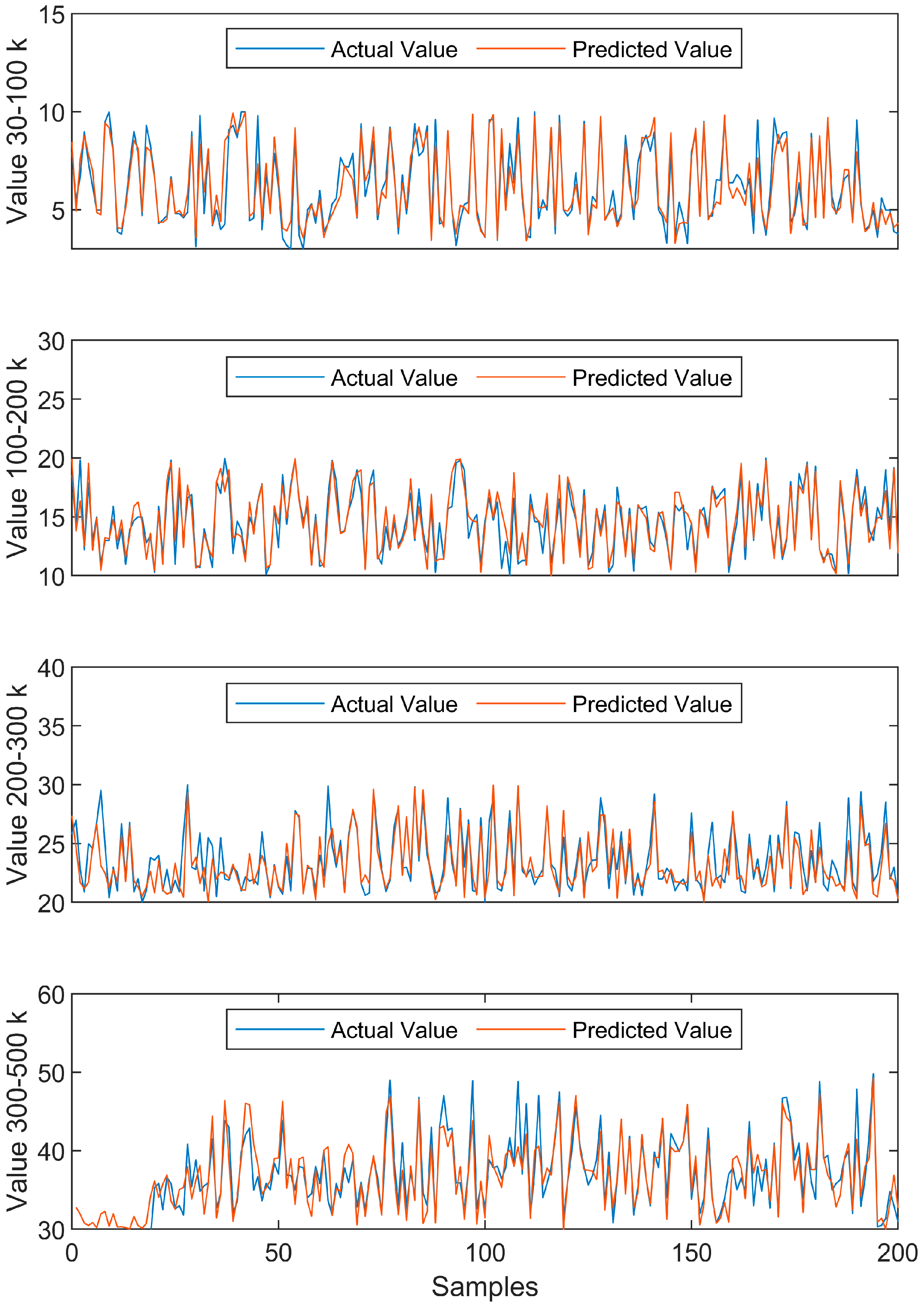
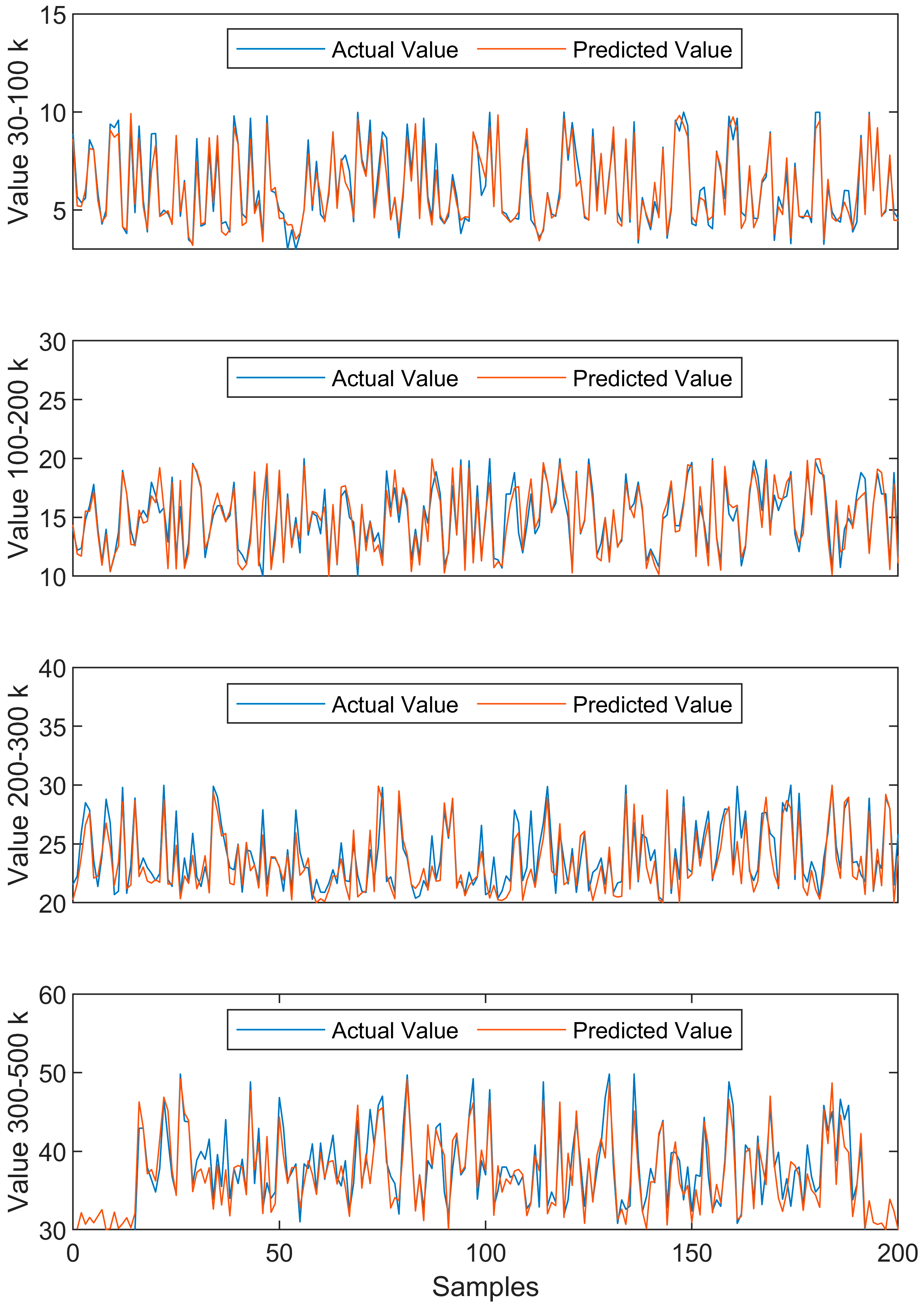
4.3. Price Updating with Extra Training

Due to the relatively low prediction accuracy of the used EVs, we proposed a price-updating strategy according to the used EV data crawled at different times. We believe that long-term unsold EV prices may not match the current selling prices of similar models, leading to low prediction accuracy. Therefore, we propose a strategy of regularly updating prices which needs three rounds of training and testing (Methods). As is shown in

Table 6. Evaluation of updated model with different methods.

Price Range	Method	Training and Testing (1st)	Training and Testing (2nd)	Training and Testing (3rd)
30–100 k	MSE	0.615	0.581	0.540
	RMSE	0.784	0.762	0.735
	MAE	0.571	0.550	0.502
	R2	0.864	0.866	0.866
100–200 k	MSE	1.650	1.281	1.321
	RMSE	1.284	1.132	1.149
	MAE	0.916	0.807	0.825
	R2	0.811	0.847	0.839
200–300 k	MSE	2.566	3.076	2.545
	RMSE	1.602	1.754	1.595
	MAE	1.093	1.281	1.163
	R2	0.649	0.588	0.663
300–500	MSE	7.484	6.805	6.881
	RMSE	2.736	2.609	2.623
	MAE	1.827	1.833	1.928
	R2	0.683	0.694	0.693
30–500 k	MSE	1.843	1.733	1.651
	RMSE	1.358	1.317	1.285
	MAE	0.886	0.873	0.849
	R2	0.978	0.979	0.980

, almost all the indexes including MSE, RMSE, MAE and R² are improved in each price range after 2nd and 3rd time of training and especially the performance of indexes for the overall price range (30–500 k) is promoted after the 3rd time of modeling. Moreover, the regression accuracy after 3 times of modeling shows that the improvement in accuracy mainly comes from the prediction accuracy of low-priced vehicle models (

Table 7. Regression accuracy of the updated model.

Price Range	Acc. Within	Training and Testing (1st)	Training and Testing (2nd)	Training and Testing (3rd)
30–100 k	5%	0.364	0.401	0.442
	10%	0.652	0.677	0.745
100–200 k	5%	0.545	0.589	0.563
	10%	0.816	0.863	0.864
200–300 k	5%	0.688	0.605	0.621
	10%	0.899	0.871	0.897
300–500 k	5%	0.655	0.623	0.612
	10%	0.879	0.880	0.872
30–500 k	5%	0.515	0.521	0.534
	10%	0.777	0.795	0.828

). Such a result indicates that lower-priced EV models are more difficult to price in the second-hand market.

We also plot the prediction value and the actual value of the used EV prices for four different price ranges across three pricing updating sections (Figure 4, Figure 5 and Figure 6). However, the improvement seems not significantly large. It may be due to the large price range of the used EVs. For a used EV pricing 50 k, 5 k price adjustment accounts for 10% of its sell price, whereas for a used EV pricing 500 k, it only occupies 1% of this price when there is a 5-k price fluctuation.

5. Discussion

Compared to second-hand gasoline cars, the price of second-hand EVs is more susceptible to impact, usually manifested as a significant depreciation once purchased. The reasons are as follows. First, EV technology is rapidly evolving, leading to continuous improvements in battery efficiency, range, and features. Older EV models may lack the latest advancements, making them less desirable in the used market and impacting their pricing. Second, government incentives and subsidies for purchasing new EVs can influence the pricing of used EVs indirectly. When incentives are available for new EV purchases, it may lead to higher demand for new EVs, affecting the supply and demand dynamics of the used EV market. For example, the Ministry of Commerce, the Ministry of Finance, and seven other departments recently jointly issued the Implementation Rules for Subsidies for Automobile Trade-ins, which were released to the public on 26 April 2024 [32]. It clarifies the subsidy policy for automobile trade-ins: individual consumers who scrap old fuel passenger cars with National III-and-below emission standards or used EVs registered before 30 April 2018 and purchase new energy passenger cars will receive a one-time fixed subsidy. In addition, the government’s policy on EVs is not limited to subsidies and incentives which will patently promote the development of EV markets. The policy for EVs is a complex system concerning governments at various levels with multiple purposes [33]. For example, the early policies of new energy vehicles in Hebei Province were mainly aimed at reducing air pollution since 2015 [33,34]. From the view of the Jing-Jin-Ji region, the government’s policy aims to facilitate infrastructure development [33]. It is reported that the charging discount and infrastructure construction subsidy can more effectively promote EV sale volume than the purchase subsidy policy from the investigation of 88 Chinese pilot cities [35] and the consumers’ perceived inconvenience of using EVs should also be considered during the policy-making process [36]. Although such an investigation occurred before 2019, it can also provide some inspiration for the upcoming massive used EV market under a series of government policies. For example, as the EV market transitions from an incremental market to a stock one [37], the government must introduce policies to protect the prices of used EVs and encourage people to purchase new EVs. At the same time, the development of used EVs may also rely on Internet thinking; for example, commercializing personal charging stations which are all dependent on the adjustment of government policies. Third, the battery degradation and the popularity of charging facilities are the main factors that impact the used EVs’ pricing. Areas with well-developed charging networks may see higher demand for EVs, leading to higher resale values, while regions with limited charging options may experience lower demand and consequently lower prices for used EVs. Fourth, the imperfect after-sales service of automobiles also restricts the price of second-hand EVs. There are many preferential policies for purchasing a new EV, such as free rescue and exclusive charging stations. However, after reselling a used EV, the next owner may not be able to enjoy these policies and services. Last but not least, unlike traditional fuel vehicles, the popularity of EVs is still not high. As of the end of 2022, the total number of EVs in China reached 13.1 million, accounting for 4.10% of the total number of vehicles [38,39]. In summary, reasonable pricing of used EVs is crucial as it not only affects individuals’ EV adoption behavior [40,41], but also affects the country’s deployment of smart grids [42,43].

Due to so many factors influencing the used EV pricing, it is difficult to estimate the price merely by virtue of experience and thus big data and machine learning methods have been applied to predict used car prices [23,44]. The methods like neural networks, random forest regressors, lightGBM, decision trees, and linear regression are always adopted and as a consequence, evaluation indexes like MAE, RMSE and R² are employed. It is noted that market dynamics which include economic factors, government policies, market participants’ preferences, and technological advancements decide the EV pricing [45,46,47]. Meanwhile, internal factors of market dynamics can also influence each other, leading to price fluctuations. For example, the investors of the charging station are inclined to create a monopolistic market atmosphere where insufficient charging stations are provided which leads to a slow diffusion of EVs. However, reasonable policy intervention can effectively prevent the decline of the EV industry [48,49]. The above dynamic factors will be mixed with more complex circumstances like safety factors and also be transmitted to the used EV market. Moreover, in contrast to the new EV market, the used EV sale depends more on e-commerce, especially in China, and thus consumer trust is also an important factor that influences the used EV market [50]. However, for consumers, the most intuitive way to evaluate the quality of a prediction model is the gap between predicted and actual prices. Here, we use a tolerance that confines the predicted price error to 5% or 10% to demonstrate the accuracy of prediction. It is obvious that even with a sufficient sample size (Figure 1 and Table 1), the model’s prediction of prices for low-priced used EVs is still very inaccurate (Table 3 and Table 7). It may be due to the fact that it is difficult to have a reasonable empirical formula that matches low-priced used cars (30–100 k RMB), and used car dealers also give a price based on the quotes of others. In this situation, the quotes from others become very important, and continuously obtaining prices for similar electric vehicles and modifying the model becomes the key to accurately predicting as much as possible. On the other hand, the price prediction of second-hand EVs for models ranging from 200 k to 500 k RMB with a prediction error of 10% is relatively accurate (nearly 90%, Table 7) and multiple modeling with re-crawling did not promote the improvement of accuracy. This result indicates that the prices of relatively high-priced used EVs fluctuate steadily and are more in line with the psychological price range of both buyers and sellers.

In sensitivity analysis for the price prediction model of used EVs, tracking the model’s performance across various scenarios over time provides deeper insights into its dynamics. This approach helps identify pivotal features that can facilitate data acquisition strategies and decision-making, enhancing the model’s resilience and accuracy. Since textual features exert negligible influence on model outcomes and are characteristically sparse, they are typically excluded from sensitivity analyses. Instead, we concentrate on numerical features to generate partial dependence plots (PDP), employing GBRT as our predictive model for price forecasting.

PDP visualizes the marginal impact of a EV’s characteristic on the predictions emanating from a machine learning algorithm. The marginal effect delineates the association between a unitary alteration in a predictive variable and the resultant shift in the dependent variable. In this context, we are examining a univariate PDP, which depicts the interplay between a machine learning model and an individual feature, while disregarding the influence of all other features. The x-axis shows possible values for a particular feature, whereas the y-axis indicates the mean forecasted value of the machine learning model’s prediction function for each discrete value along the x-axis.

The PDP curve reveals that registration time has a progressively detrimental effect on price (Figure 7). This suggests that the worth or operational efficacy of a vehicle declines as its service life advances. Likewise, the PDP curve portrays a negative correlation with mileage, implying that cars with substantial mileage records are apt to exhibit reduced worth or performance. In contrast, the suggested price’s PDP curve manifests a positive correlation, signifying that vehicles with elevated suggested prices are likely to embody superior worth or performance. The influence of standard capacity (battery capacity) on price is not linear and exhibits significant fluctuations. As the volume of the car increases, so does the price, indicating that larger vehicles tend to be more expensive. From 3000 to 5000 revolutions per minute (rpm), the price gradually rises, suggesting that vehicles with higher motor speeds are priced higher for used EVs.

There are also limitations to this work. Firstly, crawling data requires a certain amount of time, making it difficult to ensure that it is not updated while crawling data. Secondly, we only crawled data from one website, which may result in insufficient data volume. However, it is difficult to ensure that data crawled from multiple websites is not duplicated. Therefore, further research on data crawling is needed to ensure sufficient and effective data is obtained. Thirdly, the policy factors are difficult to be contained in the proposed model. Previously, Yu et al. proposed a model of a sequential game structure of a two-sided market which considers the intervention effect of government policy to the EV market [49]. Nevertheless, our model relies more on data, and sudden changes in data caused by policies are difficult to detect, so time factors related to that sudden change will be considered in future work. In addition, a website containing specific predicted prices will be promoted so that interested parties can obtain price prediction ranges by entering the necessary parameters. It can be foreseen that the used EV market needs not only price prediction but also comprehensive services like security assessment, complete testing services, etc., which can build trust between buyers and sellers.

6. Conclusions

In this study, we compare different methods for used EV price prediction. Then, we propose a circular pricing method that uses the GBRT method for modeling and involves multiple EV data crawls and deletions. Our method can achieve an accuracy of 82% in predicting the overall price of EVs (30–500 k RMB) with a prediction error of 10%. Although the accuracy of predictions needs further improvement, our model provides buyers and used car dealers with price references for used EVs under the vast amount of data.

References

1. Zhang, W.; Fang, X.; Sun, C. The alternative path for fossil oil: Electric vehicles or hydrogen fuel cell vehicles? J. Environ. Manag. 2023, 341, 118019. [Google Scholar] [CrossRef] [PubMed]
2. Zhang, T.; Burke, P.J.; Wang, Q. Effectiveness of electric vehicle subsidies in China: A three-dimensional panel study. Resour. Energy Econ. 2024, 76, 101424. [Google Scholar] [CrossRef]
3. Wang, N.; Tang, L.; Zhang, W.; Guo, J. How to face the challenges caused by the abolishment of subsidies for electric vehicles in China? Energy 2019, 166, 359–372. [Google Scholar] [CrossRef]
4. Jones, B.; Nguyen-Tien, V.; Elliott, R.J.R. The electric vehicle revolution: Critical material supply chains, trade and development. World Econ. 2023, 46, 2–26. [Google Scholar] [CrossRef]
5. Wang, S.; Yu, J. Evaluating the electric vehicle popularization trend in China after 2020 and its challenges in the recycling industry. Waste Manag. Res. 2021, 39, 818–827. [Google Scholar] [CrossRef]
6. Hu, S.; Wen, Z. Why does the informal sector of end-of-life vehicle treatment thrive? A case study of China and lessons for developing countries in motorization process. Resour. Conserv. Recycl. 2015, 95, 91–99. [Google Scholar] [CrossRef]
7. Yechiam, E.; Abofol, T.; Pachur, T. The Seller’s Sense: Buying–Selling Perspective Affects the Sensitivity to Expected Value Differences. J. Behav. Decis. Mak. 2017, 30, 197–208. [Google Scholar] [CrossRef]
8. Car Review. BMW i3 Has a Significant Price Cut, Which One Is More Attractive than the Xiaomi SU7? Available online: https://new.qq.com/rain/a/20240606A03OQD00 (accessed on 29 June 2024).
9. Gabriel, P.; Helena, N. Second-hand electrical vehicles: A first look at the secondary market of modern EVs. Int. J. Electr. Hybrid Veh. 2018, 10, 236–252. [Google Scholar] [CrossRef]
10. Rogoff, K.; Yang, Y. Rethinking China’s growth. Econ. Policy 2024. [Google Scholar] [CrossRef]
11. Storchmann, K. On the depreciation of automobiles: An international comparison. Transportation 2004, 31, 371–408. [Google Scholar] [CrossRef]
12. Cramer, J.S. The depreciation and mortality of motor-cars. J. R. Stat. Soc. Ser. A Stat. Soc. 1958, 121, 18–46. [Google Scholar] [CrossRef]
13. Venkatasubbu, P.; Ganesh, M. Used cars price prediction using supervised learning techniques. Int. J. Eng. Adv. Technol. 2019, 9, 216–223. [Google Scholar] [CrossRef]
14. Wu, J.D.; Hsu, C.C.; Chen, H.C. An expert system of price forecasting for used cars using adaptive neuro-fuzzy inference. Expert Syst. Appl. 2009, 36, 7809–7817. [Google Scholar] [CrossRef]
15. Pandey, A.; Rastogi, V.; Singh, S. Car’s selling price prediction using random forest machine learning algorithm. In Proceedings of the 5th International Conference on Next Generation Computing Technologies (NGCT-2019), Misraspatti, India, 20–21 December 2019. [Google Scholar]
16. Samruddhi, K.; Kumar, R.A. Used car price prediction using k-nearest neighbor based model. Int. J. Innov. Res. Appl. Sci. Eng. 2020, 4, 629–632. [Google Scholar]
17. Gajera, P.; Gondaliya, A.; Kavathiya, J. Old car price prediction with machine learning. Int. Res. J. Mod. Eng. Technol. Sci. 2021, 3, 284–290. [Google Scholar]
18. Longani, C.; Prasad Potharaju, S.; Deore, S. Price prediction for pre-owned cars using ensemble machine learning techniques. In Recent Trends in Intensive Computing; IOS Press: Amsterdam, The Netherlands, 2021; pp. 178–187. [Google Scholar]
19. Gegic, E.; Isakovic, B.; Keco, D.; Masetic, Z.; Kevric, J. Car price prediction using machine learning techniques. TEM J. 2019, 8, 113. [Google Scholar]
20. Cui, B.; Ye, Z.; Zhao, H.; Renqing, Z.; Meng, L.; Yang, Y. Used car price prediction based on the iterative framework of XGBoost+ LightGBM. Electronics 2022, 11, 2932. [Google Scholar] [CrossRef]
21. Muti, S.; Yıldız, K. Using linear regression for used car price prediction. Int. J. Comput. Exp. Sci. Eng. 2023, 9, 11–16. [Google Scholar] [CrossRef]
22. Huang, J.; Saw, S.N.; Feng, W.; Jiang, Y.; Yang, R.; Qin, Y.; Seng, L.S. A Latent Factor-Based Bayesian Neural Networks Model in Cloud Platform for Used Car Price Prediction. IEEE Trans. Eng. Manag. 2023. [Google Scholar] [CrossRef]
23. Pillai, A.S. A Deep Learning Approach for Used Car Price Prediction. J. Sci. Technol. 2022, 3, 31–50. [Google Scholar]
24. Liu, E.; Li, J.; Zheng, A.; Liu, H.; Jiang, T. Research on the Prediction Model of the Used Car Price in View of the PSO-GRA-BP Neural Network. Sustainability 2022, 14, 8993. [Google Scholar] [CrossRef]
25. Jin, C. Price Prediction of Used Cars Using Machine Learning. In Proceedings of the 2021 IEEE International Conference on Emergency Science and Information Technology (ICESIT), Chongqing, China, 22–24 November 2021; pp. 223–230. [Google Scholar]
26. Bukvić, L.; Pašagić Škrinjar, J.; Fratrović, T.; Abramović, B.J.S. Price prediction and classification of used-vehicles using supervised machine learning. Sustainability 2022, 14, 17034. [Google Scholar] [CrossRef]
27. Wang, Z.; Ching, T.W.; Huang, S.; Wang, H.; Xu, T. Challenges faced by electric vehicle motors and their solutions. IEEE Access 2020, 9, 5228–5249. [Google Scholar] [CrossRef]
28. Yang, L.; Wu, H.; Jin, X.; Zheng, P.; Hu, S.; Xu, X.; Yu, W.; Yan, J. Study of cardiovascular disease prediction model based on random forest in eastern China. Sci. Rep. 2020, 10, 5245. [Google Scholar] [CrossRef] [PubMed]
29. Kuhn, M.; Johnson, K. Applied Predictive Modeling; Springer: New York, NY, USA, 2013; Volume 26. [Google Scholar]
30. Awad, M.; Khanna, R.; Awad, M.; Khanna, R. Support vector regression. In Efficient Learning Machines: Theories, Concepts, and Applications for Engineers and System Designers; Apress: Berkeley, CA, USA, 2015; pp. 67–80. [Google Scholar]
31. Zhu, G.; Li, Q.; Zhao, W.; Lv, X.; Qian, C.; Qian, Q. Tropical Cyclones Intensity Prediction in the Western North Pacific Using Gradient Boosted Regression Tree Model. Front. Earth Sci. 2022, 10, 929115. [Google Scholar] [CrossRef]
32. Financial Aid Backs Equipment Renewal. 2024. Available online: http://en.people.cn/n3/2024/0412/c90000-20156152.html (accessed on 29 June 2024).
33. Zhang, X.; Bai, X. Incentive policies from 2006 to 2016 and new energy vehicle adoption in 2010–2020 in China. Renew. Sustain. Energy Rev. 2017, 70, 24–43. [Google Scholar] [CrossRef]
34. Ji, W.; Zhao, K.; Zhao, B. The trend of natural ventilation potential in 74 Chinese cities from 2014 to 2019: Impact of air pollution and climate change. Build. Environ. 2022, 218, 109146. [Google Scholar] [CrossRef]
35. Qiu, Y.Q.; Zhou, P.; Sun, H.C. Assessing the effectiveness of city-level electric vehicle policies in China. Energy Policy 2019, 130, 22–31. [Google Scholar] [CrossRef]
36. Qian, L.; Grisolía, J.M.; Soopramanien, D. The impact of service and government-policy attributes on consumer preferences for electric vehicles in China. Transp. Res. Part A Policy Pract. 2019, 122, 70–84. [Google Scholar] [CrossRef]
37. Yang, Z. The development of new energy vehicles will enter a period of deep adjustment. China Energy News, 8 January 2024. [Google Scholar]
38. Yearender: China’s New Energy Vehicle Industry in Growth Fast Lane. Available online: https://english.news.cn/20221229/82c05e5ef538408b87fb77ba71b854e9/c.html (accessed on 29 June 2024).
39. Jia, J.; Shi, B.; Che, F.; Zhang, H. Predicting the Regional Adoption of Electric Vehicle (EV) With Comprehensive Models. IEEE Access 2020, 8, 147275–147285. [Google Scholar] [CrossRef]
40. Li, W.; Long, R.; Chen, H.; Geng, J. A review of factors influencing consumer intentions to adopt battery electric vehicles. Renew. Sustain. Energy Rev. 2017, 78, 318–328. [Google Scholar] [CrossRef]
41. Cecere, G.; Corrocher, N.; Guerzoni, M. Price or performance? A probabilistic choice analysis of the intention to buy electric vehicles in European countries. Energy Policy 2018, 118, 19–32. [Google Scholar] [CrossRef]
42. Mwasilu, F.; Justo, J.J.; Kim, E.-K.; Do, T.D.; Jung, J.-W. Electric vehicles and smart grid interaction: A review on vehicle to grid and renewable energy sources integration. Renew. Sustain. Energy Rev. 2014, 34, 501–516. [Google Scholar] [CrossRef]
43. Liu, L.; Kong, F.; Liu, X.; Peng, Y.; Wang, Q. A review on electric vehicles interacting with renewable energy in smart grid. Renew. Sustain. Energy Rev. 2015, 51, 648–661. [Google Scholar] [CrossRef]
44. Chandak, A.; Ganorkar, P.; Sharma, S.; Bagmar, A.; Tiwari, S. Car price prediction using machine learning. Int. J. Comput. Sci. Eng. 2019, 7, 444–450. [Google Scholar] [CrossRef]
45. Ouyang, D.; Zhang, Q.; Ou, X. Review of Market Surveys on Consumer Behavior of Purchasing and Using Electric Vehicle in China. Energy Procedia 2018, 152, 612–617. [Google Scholar] [CrossRef]
46. Baars, J.; Domenech, T.; Bleischwitz, R.; Melin, H.E.; Heidrich, O. Circular economy strategies for electric vehicle batteries reduce reliance on raw materials. Nat. Sustain. 2021, 4, 71–79. [Google Scholar] [CrossRef]
47. Xiao, G.; Xiao, Y.; Shu, Y.; Ni, A.; Jiang, Z. Technical and economic analysis of battery electric buses with different charging rates. Transp. Res. Part D Transp. Environ. 2024, 132, 104254. [Google Scholar] [CrossRef]
48. Li, S.; Tong, L.; Xing, J.; Zhou, Y. The Market for Electric Vehicles: Indirect Network Effects and Policy Design. SSRN Electron. J. 2014. [Google Scholar] [CrossRef]
49. Yu, Z.; Li, S.; Tong, L. Market dynamics and indirect network effects in electric vehicle diffusion. Transp. Res. Part D Transp. Environ. 2016, 47, 336–356. [Google Scholar] [CrossRef]
50. Li, X.; Ma, J.; Zhou, X.; Yuan, R. Research on Consumer Trust Mechanism in China’s B2C E-Commerce Platform for Second-Hand Cars. Sustainability 2023, 15, 4244. [Google Scholar] [CrossRef]
Figure 1. Data preprocessing procedure and EV price distribution: (a) data crawling and preprocessing procedure; (b) number of EVs in different price ranges.
Sustainability 16 05761 g001
Figure 2. Correlation of different numerical features: (a), eight features; (b) power and torque are combined as speed.
Sustainability 16 05761 g002
Figure 3. Price updating strategy.
Sustainability 16 05761 g003
Figure 4. First–round training results for different price range EVs.
Sustainability 16 05761 g004
Figure 5. Second–round training results for different price range EVs.
Sustainability 16 05761 g005
Figure 6. Third–round training results for different price range EVs.
Sustainability 16 05761 g006
Figure 7. PDP analysis for used EV price with GBRT.
Sustainability 16 05761 g007