Abstract
Inventory management is crucial for companies to minimize unnecessary costs associated with overstocking or understocking items. Utilizing the economic order quantity (EOQ) to minimize total costs is a key decision in inventory management, particularly in achieving a sustainable supply chain. The classical EOQ formula is rarely applicable in practice. For example, suppliers may enforce a minimum order quantity (MOQ) that is much larger than the EOQ. Some conditions such as imperfect quality and growing items represent variants of EOQ. Moreover, some requirements, such as the reduction of CO2 emissions, can alter the formula. Moreover, disruptions in the supply chain, such as COVID-19, can affect the formula. This study investigates which requirements must be considered during the calculation of the EOQ. Based on a literature review, 18 requirements that could alter the EOQ formula were identified. The level of coverage for these requirements has been tracked in the literature. Research gaps were presented to be investigated in future research. The analysis revealed that, despite their importance, at least 11 requirements have seldom been explored in the literature. Among these, topics such as EOQ in Industry 4.0, practical EOQ, and resilient EOQ have been identified as promising areas for future research.
1. Introduction
Economic order quantity (EOQ) is the optimal number of items a company should buy to meet customer demand while keeping costs low. It helps balance the costs of storing items, running out of stock, and placing orders [1]. EOQ considers the best time to reorder, the cost of placing an order, and the cost of storing the items. Traditional EOQ models consider the trade-off between ordering and storage costs [2]. The optimal EOQ is essential for maintaining smooth material flow, which is crucial for any production or retail facility. Even though the concept of EOQ was introduced more than a century ago by Harris in 1913, there are still many research gaps. This is because of practical considerations, recent trends in digitalization and sustainability, supply chain disruptions, and the difficulty of estimating input parameters. Some variants of the original EOQ have been extensively investigated in the literature. These variants include imperfect quality, variable demand, discounts, shortages, growing items, and deteriorating items. Some studies have investigated two or more requirements in the same paper, such as the study by [3], which examined EOQ in the context of sustainability and imperfect quality. However, other variants have been overlooked by researchers and can hardly be found in the literature. These variants include uncertain supply, EOQ based on logistics units, and easy-to-calculate EOQ. Furthermore, little has been published regarding the most efficient methods for determining input parameters, such as inventory holding costs and ordering costs. A major problem that is usually ignored is the minimum order quantity (MOQ) imposed by suppliers [4,5]. If the EOQ is less than the MOQ, there is no point in the complex calculations of the EOQ.
1.1. Research Gap
There has been insufficient empirical research to determine the EOQ for different conditions. Surveys on different practices for finding the EOQ and its parameters have also been neglected in the literature. In this study, we explain the research gaps that should be addressed in future research. Recent attempts to review EOQ have been limited. Unfortunately, none of these review studies are comprehensive. They usually consider the EOQ problem from a certain perspective. Furthermore, little research has explained research gaps or suggested directions for future research. For example, Jaber and Peltokorpi [6] reviewed EOQ/EPQ models with product recovery from a mathematical point of view. Bakker et al. [7] reviewed inventory control of perishable items (deteriorating inventory). They focused on system characteristics such as price discounts, back-ordering or lost sales, and single or multiple items. It is difficult to define the values of certain factors in inventory management models. Fuzzy models are important in these situations [8]. An analysis of possible parameters of existing inventory control models was presented by Ziukov [9], who presented an overview of the existing literature, focusing on descriptions of the types of inventory control models. Thinakaran et al. [10] surveyed the inventory model of the EOQ under full and partial backorder conditions. However, they did not mention any research gaps.
1.2. Aim and Contribution
The aim of this research is not to summarize all the studies about EOQ or even the recent studies about it, but to focus more on the different variants of the original model and practical considerations that need more attention for future research. More emphasis is placed on the effect of recent disruptions in supply chains, environmental considerations, COVID-19, and Industry 4.0 on the EOQ model.
The contributions of this study are threefold. Firstly, it draws researchers’ attention to incorporating recent trends such as Industry 4.0 and sustainability into the EOQ formula. Secondly, it emphasizes the practical considerations that have been overlooked by researchers and need to be explored in future studies. Lastly, the study is comprehensive, addressing all the requirements of the EOQ formula.
1.3. Research Questions
The research questions in this study are:
- Which EOQ variants and practical considerations (requirements) are most important, especially those related to recent trends in digitalization and supply chain disruptions?
- Which of these requirements is not sufficiently covered in the literature and needs more attention by researchers in the future?
- Are there critical variants that were not covered at all in the literature?
After this introduction, Section 2 covers the theoretical background and motivation. Section 3 outlines the methodology, which is based on a systematic literature review. Section 4 presents the results and discusses the implications of the study. Finally, Section 5 provides the conclusions and recommendations for future research.
2. Research Background and Motivation
The EOQ model was first presented by Harris in 1913. The formula is
where K is ordering cost per order, d is demand in units per unit time, and h is inventory holding cost per unit held per unit time. The term “holding costs” (or “carrying costs”) refers to the costs associated with storage, material handling, insurance, taxes, obsolescence, theft, and interest on purchases. As inventory levels increase, costs increase. Generally, holding costs are calculated as a percentage of the unit value rather than as individual costs. The “ordering cost” refers to the cost of placing an order for a product. These expenses include order communication, allowances for purchase officers, order printing and stationery, inspection costs, product delivery, and transportation costs [11]. These costs are assumed to remain constant and unchanged throughout the period, regardless of the number of orders placed.
There are some assumptions in the basic model such as constant demand, instantaneous lead time, constant costs, no shortage is allowed, and the entire batch comes at the same moment. Some variants of the basic model appeared in the early stages, considering factors such as backorder and inflation. Backorder constraints can, for example, be the total or average number of backorders at any time point. Buzacott [12] investigated the effect of inflation. Moreover, Ballentine et al. [13] combined ABC analysis and EOQ and found that most of the savings were from low-value frequently demanded items. Uncertainty in the input data such as the demand rate, order cost, and holding cost rate have been investigated in many studies such as Yu [14], where a robust approach of inventory policy that performs well under different input data scenarios was presented. Uncertainty increases in newly opened businesses and brand new products just entering the market, or when competition is fierce. Other attempts to fit various requirements include Chen and Liao [15] to include intermediary firms and Drezner et al. [16] to consider when two products are required, and it is possible to substitute one product for another. Additional variants include imperfect quality [17], reusable products [18], and growing products like poultry and livestock, whose inventory levels increase in weight over time [19]. Recently, more attention has been paid to environmental issues and their effects on inventory management systems [20,21]. Battini et al. [22] formulated a sustainable EOQ model incorporating environmental factors such as carbon emissions. The study aimed to balance economic and environmental costs in determining the optimal order quantity. Empirical data showed the trade-offs between economic and environmental costs. For example, integrating carbon costs resulted in a 5–10% increase in EOQ compared to the traditional model. Some studies combined multiple variants or trends, such as Gharaei and Almehdawe [23], who considered growing items and the environmental impacts of GHGs emitted during manure production, fermentation processes, and transportation. Lee et al. [24] considered the sustainable EOQ in the case of stochastic lead time. Moreover, the emerging technologies of Industry 4.0 affected inventory management [25].
Figure 1 shows the trend of publications about EOQ in the new millennium as found in Google Scholar. Figure 2 shows the number of publications that contain both the EOQ and sustainability principles or EOQ and Industry 4.0. Even though the term Industry 4.0 started in 2011, its technologies started earlier. Therefore, the following keywords were used to look for both principles in any part of the studies: (“internet of things” OR iot OR cps OR “cyber physical system” OR “smart factory” OR “industry 4” OR “I 4.0” OR “the fourth industrial revolution” OR “smart manufacturing” OR RFID AND “economic order quantity”).
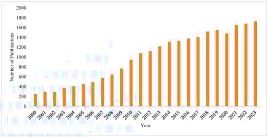
Figure 1.
Number of publications of EOQ over time.
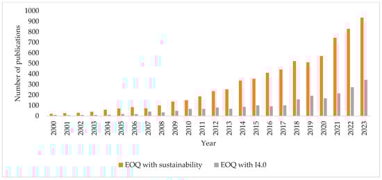
Figure 2.
Number of publications about both EOQ and sustainability/I4.0 over time.
The two figures show a fast increase in the number of publications over time. In 2000, the number of publications containing both EOQ and sustainability was only 8% of the total number of publications about EOQ. This percentage increased to 54%. Industry 4.0 started to increase especially starting in 2018, but with less attention by authors than sustainability.
The effect of COVID-19 has significantly changed the perspective of supply chain and inventory management [26,27]. A study by Hidayatuloh et al. [28] investigated the effect of uncertainties during the COVID-19 pandemic on the EOQ formula. The study utilized a case study approach in a pharmacy and employed Monte Carlo simulation to analyze the impact of spike demand, stockouts, and disruptions. The detailed simulation results indicated the range of EOQs under different scenarios of demand and supply disruptions. For instance, during peak COVID-19 periods, the EOQ had to be increased by 20–30% to prevent stockouts, while in periods of stabilized demand, the EOQ could be reduced by 10–15% to minimize holding costs. Recent political conflicts have also affected inventory management best practices [29]. Therefore, new variants of the original EOQ have yet to be developed. These new variants will provide a better way to determine the EOQ. They will enable businesses to maximize their inventory efficiency and reduce costs. In addition, they will offer improved customer service and satisfaction.
However, to date, no study has listed all the EOQ variants. Therefore, this study presents a variety of variants of the EOQ model with some examples from the literature and shows the gaps in the research. Some variants have only been considered by a few researchers, which opens the door to possibilities for future research.
3. Materials and Methods
The methodology depends on a systematic literature review of the different variants, especially those related to recent changes in inventory management. Christata and Daryanto [30] reviewed the literature on single-echelon inventory models that considered carbon emissions between 2010 and 2020. They identified thirty-three relevant articles and recommended that further research be conducted on low-carbon EOQ models. Poswal et al. [31] reviewed fuzzy EOQ models in shortage situations.
In this study, Google Scholar was used as the search engine because it covers several databases [32]. Studies from many journals were considered. Google Scholar includes a wide variety of academic and scholarly sources. It gathers articles from major academic publishers like Elsevier, Springer, Wiley, and Taylor & Francis. It also includes research papers and theses from universities, publications from professional societies such as IEEE, ACM, and the American Chemical Society, as well as papers from preprint servers like arXiv, SSRN, and bioRxiv. The idea is not to cover all EOQ-related studies but to concentrate more on studies related to areas not covered enough in the literature despite their importance. Biggs et al. [33] examined ordering costs based on the feedback of companies. No attempt was made after that to find ordering costs based on feedback from the companies. Another empirical study is that by Azzi et al. [34], who calculated inventory holding costs. However, such costs are difficult to measure. Therefore, research on best practices for estimating them is very important.
This paper utilized well-cited studies. Except for the studies published in the last year, studies should usually have at least 10 citations. For example, even though the growing items concept in EOQ is relatively new, many studies have covered it. Therefore, it is assumed that the chance for gaps in such a variant is low. In this study, a variant of EOQ is called so if some conditions are agreed on in the literature about certain conditions such as imperfect quality, where some parts are defective and need to be replaced after inspection. Being well investigated by previous studies does not necessarily mean there is no chance of future research about that variant. However, it may require deeper investigation and possibly more complex computations. In this study, a topic is considered well-covered if there are at least 10 high-quality papers about it.
The following general steps are followed in this study:
- Select Google Scholar as the primary search engine;
- Literature review of EOQ;
- Identify special requirements: variants, practical considerations, recent disruption, recent technologies, and recent trends;
- Examine which requirements are covered enough and which are not;
- Determine research gaps in those requirements not covered enough.
Figure 3 illustrates the study methodology. A systematic literature review is needed. The initial literature review is necessary to determine the different EOQ requirements. These requirements are divided into four groups. Figure 3 shows that there is no need to cover all the papers about a certain requirement if it is well covered. However, if only a few studies investigate a certain requirement, then all of them should be screened and tested for possible gaps for future research. The rest of the methodology steps are explained in the following subsections.
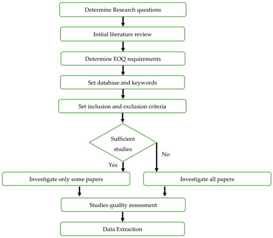
Figure 3.
Research methodology.
3.1. Data Sources
Google Scholar was used as the search engine because it covers most research articles and is easy to use.
3.1.1. Keywords
The keywords vary based on different requirements. In the previous section, the keywords used to combine Industry 4.0 and EOQ were presented. Boolean operators (AND, OR) were utilized: AND is used to combine EOQ with other principles such as Industry 4.0, while OR is used when multiple words can represent the same concept.
3.1.2. Inclusion Criteria
The papers should be published in journals, conferences, or book chapters and must be written in English. They should also address the requirement being evaluated. Using keywords alone is insufficient; manual scanning of the papers is necessary to ensure they adequately cover the needed requirements. Studies typically explore methods to calculate EOQ under various conditions using techniques such as analytical investigation. If multiple papers address a specific requirement, the first few results are usually sufficient, as the objective is to identify requirements that need deeper investigation by researchers in the future.
3.1.3. Exclusion Criteria
Book reviews and reports are excluded because they typically lack peer review. Studies older than 30 years are usually excluded unless the total number of references for a certain requirement is low (for example, fewer than 10). However, exceptionally important papers considered major references can still be used. Review papers are typically excluded unless they are used as general references. Priority is given to empirical research. Papers in languages other than English are also excluded.
3.2. Study Quality Assessment
Manual review of the papers is essential to ensure they sufficiently address the required criteria. This includes factors such as the number of citations. For instance, a paper that is 10 years old with no or few citations is typically excluded, unless there are very few papers investigating the same requirement. If the paper is from a well-known source such as Springer or Wiley, it is accepted for use. However, if the database is not well-known, careful manual scanning is necessary. Additionally, if two papers cover the same idea already well-documented in the literature, preference is given to the most recent one. Usually, papers from journals are used. However, if there is a lack of research on a certain requirement, a conference paper can be used. Non-peer-reviewed sources are avoided. Manual scanning is also used to check if the papers contain all the necessary parts, such as the introduction, methodology, results, analysis, and conclusion. It ensures the main focus of the paper is on the EOQ principle. This is because some papers only mention the EOQ principle in the literature review or references section.
3.3. Data Classification
The studies presented as examples for different requirements are from different journals. Table 1 shows some of these journals. In the “other journals” category, every journal has only one publication. This shows that the topic is discussed in a wide range of journals. In addition to journals, there are three papers from conferences. The table does not show all the references used in this paper. It only shows the classified studies, in which only few examples are mentioned about each requirement of the EOQ.

Table 1.
Journals of the classified studies.
Figure 4 shows the dot plots representing the years of publications of the references used in this paper. The figure shows that most of the references are in the last few years. Using older references is necessary sometimes to show that some variants were overlooked by researchers; hence, older studies were included.
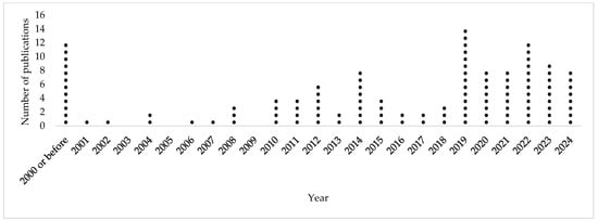
Figure 4.
Years of publications of the classified studies.
4. Results and Discussion
The requirements in Table 2 were found to be the most important. Their importance was estimated based on a literature review. Some of these requirements appeared in the literature very early, such as variable demand and variable ordering and inventory costs. On the other hand, recent trends such as sustainability and Industry 4.0 have introduced new requirements. To determine all these requirements, a comprehensive literature review was conducted to identify all possible modifications to the original formula, making it more practical and reflective of recent trends. The authors then divided these requirements into four subgroups, as shown in Table 2. Sometimes, two or more requirements can be addressed in a single paper. Due to the large number of requirements, some have been overlooked in the literature for a long time, despite their importance. For example, a variant recommended by numerous studies is considered important. Table 2 shows that most of these requirements were not covered enough by researchers in the literature. More details are given about each one of the requirements in the next subsections.
Table 2.
EOQ modeling requirements.
Table 3 shows some of the papers about each one of the requirements. Further explanation about each one is below.
Table 3.
EOQ requirements’ references.
Figure 5 shows the time context of the studies mentioned in Table 3. It only highlights the studies for the requirements that are not well-covered in the literature. Figure 5 illustrates that some requirements, such as the effect of Industry 4.0 and supply chain disruption, have garnered attention from researchers in the last 15 years. Others have been on the researchers’ agenda for decades but still have gaps in research. This reveals that some requirements have been ignored by researchers for a long time. Combining two or more requirements is recommended for future research.
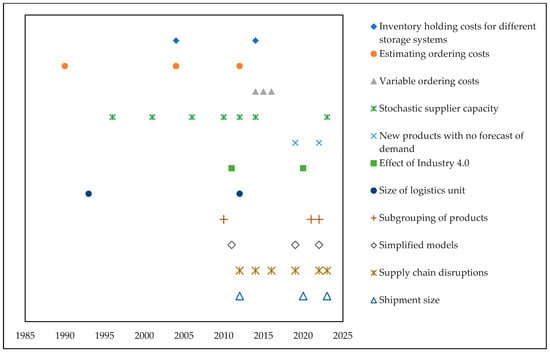
Figure 5.
Years of publication of the studies of non-well-covered requirements.
4.1. Input Parameters
4.1.1. Inventory Holding Costs for Different Storage Systems
Few empirical studies were conducted to determine inventory holding costs. Azzi et al. [34] empirically investigated inventory holding costs in companies with traditional warehouses versus those employing AS/RS. The approach, particularly in the presence of AS/RS, hinges on factors like system capacity, investment, and operational costs. According to Azzi et al. [34], storage costs decrease as AS/RS capacity increases. It was found that annual investment costs accounted for 85% of storage costs. The study by Azzi et al. [34] did not consider robotics or Industry 4.0 systems. Robotics provide flexibility in material handling. The literature has overlooked such systems. According to Choi and Enns [35], the holding costs of work-in-process inventory are less than those of finished goods because the value of finished goods is higher. Generally, determining inventory holding costs using empirical studies is a major gap in research. Best practices for estimating holding costs for different companies at different levels of technology in warehouses are needed in future research. Most studies assume the holding cost is constant or linear with time, or they use other functions.
4.1.2. Variable Holding Costs
Sometimes holding costs vary over time. Alfares and Ghaithan [36] reviewed and classified EOQ models with variable holding costs. There are three types of variable holding costs: time-dependent holding cost, stock-dependent holding cost, and multiple dependencies. Food and pharmaceuticals must be stored under refrigeration to prevent spoilage over time. Some studies investigated EOQ models for time-dependent holding costs. Setiawan [37] investigated such a case where the holding cost is a nonlinear function of time. Tripathi and Mishra [38] modeled the holding cost as a linear function of time and also assumed a time-dependent demand. Singh and Sharma [39] also assumed a time-dependent holding cost. They also considered price-dependent demand.
4.1.3. Ordering Costs
The gap in research about ordering costs is even larger than that for holding costs. For example, Biggs et al. [33] discovered that numerous companies either lack the knowledge to calculate ordering costs or do not incorporate them into their decision-making processes. They found that other companies use a rough estimation of USD 40 to USD 50 per order. However, Chen and Simchi-Levi [40] observed that part of the ordering cost is fixed, while the other part is variable. Therefore, it is proportional to the amount ordered. In many studies, ordering costs were assumed to be known and constant [41]. However, in many cases, the ordering cost follows a step function. Few attempts have been made to incorporate variable ordering costs into EOQ models. For example, Rathod and Bhathawala [42] considered stock-level dependent demand, variable holding costs, and variable ordering costs. They assumed that holding costs increase over time. Goyal et al. [43] assumed demand as a function of stock level and price. They assumed that ordering costs are a function of time. Goyal and Chauhan [44] assumed that ordering costs decrease over time because of the learning curve. They also considered the deterioration effect and stock-dependent demand.
4.2. Variants of EOQ
Except for stochastic supplier capacity and variable prices, most of the variants of EOQ were sufficiently investigated in the literature
4.2.1. Stochastic Supplier Capacity
Not much has been published about the problem of suppliers lacking capacity. A study by Arbabian and Rikhtehgar Berenji [70] investigated the inventory optimal policy for the swab demand needed for COVID-19 tests. Customers in this case are governments. Four models were developed to cover all the possible scenarios of supply (sufficient or stochastic) and demand (deterministic or stochastic). That direction of research is useful for other disruptions in supply chains such as the shortage of semiconductors and its effects on automakers. Future studies can analyze food shortages caused by current political conflicts. Before that, Wang and Gerchak [71] investigated production/inventory systems where supply is unpredictable because of unexpected breakdowns, unplanned repairs, etc. They developed a procedure for the exponential distribution of variable capacity. In addition to the exponential distribution, other studies assumed the uniform distribution for the capacity such as Erdem et al. [72] and Arbabian and Rikhtehgar Berenji [70]. Other studies investigate the variable capacity problem such as Wu [73], Wang [74], Moon et al. [75], and Wang et al. [76].
4.2.2. Variable Prices
When considering prices, most studies focused on changes in prices due to discounts. However, in many cases, the changes in prices are due to external factors such as changes in energy costs, regulations, raw materials, shortages of labor, etc. Researchers overlooked these changes, especially when they affected inventory holding costs. A study by Sodhi et al. [63] investigated the EOQ problem for maintenance, repair, and overhaul customers with discounts and the effect of these discounts on the bullwhip effect. They considered a variable purchase quantity as a function of the selling price. Taleizadeh and Pentico [64] assumed known price increases in their study about EOQ. They also assumed partial backordering. Taleizadeh et al. [65] assumed a known increase in demand when replenishment intervals are probabilistic. A study by Berling [66] investigated inventory holding costs when a stochastic purchase price follows the Ornstein–Uhlenbeck process. They modified the EOQ formula and provided simulation results. Babai et al. [67] investigated optimal ordering quantity when price and demand are correlated and change randomly over time. They compared their results to a benchmark solution. The papers that include price-dependent demand assume that larger prices will lead to lower demand [68]. In many cases, however, the rise in prices and the rise in demand occur at the same time. That happened for example in the era of COVID-19 when hygiene products witnessed hikes in prices and demand at the same time. This problem can be solved with the “resilient EOQ”.
4.2.3. Other Variants of EOQ
If the goods are damaged, deteriorated, or expired, the cost of the deteriorated goods must be included in the total inventory cost. In many cases, the life of the product is only a few days such as fresh food. Therefore, the EOQ only covers the daily demand of a few days [45]. Sharma et al. [52] introduced a salvage value parameter into the EOQ model for decaying products, addressing a demand that varies quadratically over time. The study by Limansyah et al. [46] investigated the deterioration cost when an all-units discount is offered by suppliers. Another study by Setiawan [37] investigated the EOQ for deteriorating items for the two-level inventory model using game theory. Liao et al. [37] investigated the problem of deteriorating items together with imperfect quality. They also showed a numerical example to validate the method. There are many studies about EOQ assuming variable or seasonal demand. For example, Mondal et al. [53] developed an EOQ model for seasonal products, where deterioration and backlogs were considered. Tripathi [54] assumed price-dependent demand and different functions for inventory holding costs in the model of EOQ. Geetha and Udayakumar [55] considered the EOQ model for deteriorating items and time-dependent demand because of inflation. They also considered the shortage to be permitted. A study by Verma et al. [56] examined the EOQ model with time-dependent demand for spoilable items. They maximized the profitability and used a numerical example.
There have been several studies investigating EOQ with imperfect quality. Maddah and Jaber [77] found it to be larger than the traditional EOQ when yield rate variability is low. They also considered the consolidation of several quantities with imperfect quality to be in one lot. Alfares and Afzal [17] considered the imperfect quality of growing items, but they also considered permissible shortages with complete backordering. In a study by Ayatollahi and Jafari [82], an EOQ model was developed for items with imperfect quality when there are multiple suppliers. They formulated the problem as a nonlinear programming model. Many studies investigated the growing items problem in the context of EOQ modeling, usually with other practical features. For example, Rezaei [19] examined the EOQ for growing items. At the beginning of a growing cycle, the optimal order quantity for the growing items was calculated. The optimal length of the growing cycle and profit were also calculated. The EOQ model for fast-growing newborn animals (like broiler chickens) was developed by Pourmohammad-Zia [86]. They applied a mortality rate that can be controlled by preventive practices. For the system to manage its costs effectively, it should choose a hatchery that has the lowest purchasing cost as a priority. To minimize total costs, Nobil et al. [87] investigated the slaughter age and number of chicks to purchase from the supplier. They used a five-step approach and provided a numerical example.
4.3. Trends
4.3.1. Environmental Effects
Arslan and Turkay [90] modified the traditional EOQ model to include sustainability factors. They applied the triple bottom-line accounting approach methodically. Some studies considered the effect of transportation costs and its social effect on CO2 emission such as the study by Bonney and Jaber [89]. The cost per unit distance per unit load was assumed to be the same for all trucks. Another study by Battini et al. [22] considered the different cost rates for different trucks. However, such studies did not consider the milk run, in which several items from different suppliers are transported on the same truck. Including milk run in EOQ calculations is a gap for future research. Nobil et al. [87] considered CO2 emissions from another perspective. Under a sustainable green breeding policy, the authors proposed an EOQ for growing items with a mortality function. CO2 production was assumed to be a polynomial function that depends on the age of the animals and the mortality function. A study by Jawad et al. [91] considered the hidden costs related to sustainability including environmental, labor-related, and economic effects.
4.3.2. New Products with No Forecast of Demand
Sometimes, accurate forecasting of demand is not available. A study by Chanda and Kumar [93] investigated the EOQ for new technological products based on customer feedback. Some other studies by the same two authors were conducted earlier about new products. A study by Onyenike and Ojarikre [94] considered the EOQ problem for new products with little or no historical data. In this case, the probability distribution for demand is not available or cannot easily or accurately be estimated. Therefore, they considered a fuzzy inventory model. Research in this regard is very scarce, which opens the door for future research.
4.3.3. Effect of Industry 4.0
Few studies were performed about the effect of Industry 4.0 on EOQ. The effect of the new technologies can also affect the estimation of EOQ. Bhadrachalam et al. [95] investigated the effect of the transition from non-RFID to RFID on the EOQ, assuming that RFID will reduce the lead time to almost zero. A study by Di Nardo et al. [96] investigated a dynamic EOQ model that fits into Logistics 4.0. Wang and Huang [114] introduced the concept of meta-inventory in Industry 4.0’s Cyber-Physical Production Systems, where physical items and their digital twins are part of the inventory, and quantified the impact of meta-inventory on supply chains. Another study from Shen et al. [115] examined how sustainable design can reduce environmental impact and improve the health and comfort of building occupants, leading to better financial performance. They highlighted Industry 4.0 and the circular economy as sustainable alternatives, integrating them into supply chain design and production decisions.
4.3.4. Size of Logistics Unit and Shipment Size
Research about modifying the EOQ to suit the logistics unit is very scarce. This opens the door for future research in this field. The effect of unit load size on the optimal batch size was investigated in an empirical study by Rong et al. [97], where the yearly demand was only for several pallets of drugs. The supplier may offer discounts if the batch size is standardized. A full pallet, half pallet, or even a smaller batch size were considered. Material handling of a complete pallet is easier. However, it leads to large inventory holding costs. Therefore, the optimal batch size was compared to EOQ. They found that using the traditional EOQ leads to poor results. Before that, a study by Daganzo and Newell [98] also investigated the effect of material handling, transportation, and inventory costs on the lot size. Lot sizes that can be easily handled, such as boxes and pallets, are chosen. Therefore, the lot size is not a continuous function. If orders from customers are less than a pallet size, different items are combined in a mixed-item pallet. They recommended delivering lots of unequal sizes and/or at unequal time intervals.
Very few studies considered the practical shipment size for freight transport. It is a decision made based on technical possibilities and transportation modes. In a study by Combes [110], an empirical evaluation of the simple EOQ model was conducted at a national level, over a heterogeneous sample of shipments. Moreover, shipment size modeling for intra-city shipments was conducted in the study of Sakai et al. [111]. Additionally, the estimated coefficients were compared with their theoretical values derived from a conceptual EOQ model. Depending on the model of Sakai et al. [111], a study by Jing et al. [112] optimized the shipment size to reduce the annual logistics cost of a contract, based on three cost components: inventory costs, capital cost during transportation and transportation costs. Another study by Reda et al. [113] investigated the temporal stability of shipment size choices. To determine the optimal shipment size, demand, transportation costs, ordering, and inventory costs are taken into consideration. Their results showed that shipment size decisions are not stable over time.
4.3.5. Subgrouping of Products
The subgrouping of products needs more investigation by researchers. According to Gurtu [99], holding costs vary based on different organizations and locations due to factors such as space costs and finance costs. For example, Wahab and Jaber [100] examined the EOQ when different holding costs for good and defective items were taken into account. Generally, inventories with perishable items or items that require refrigeration have a much higher inventory holding cost. In addition, obsolescence costs vary based on the item. Moreover, the weight and space required by items are different. However, sometimes, there are thousands of different items, and calculating the holding cost for each one of them is not practical. Therefore, it is important to subgroup them into a few types. In a study by Inayah et al. [101], different EOQs were found for different products based on ABC analysis. Gurtu [99] suggested using a representative item from each family to make the calculations. Different branches of a company can be divided into subgroups in the same geographical zone. In each subgroup, different holding costs can be used.
4.3.6. Simplified Models
Only a few studies were published about simplified formulas that can be easily understood by practitioners. Therefore, this is a gap in research that needs further analysis. A study by Baller and Spinler [102] investigated the possibility of obtaining EOQ with fewer data by simplifying formulas. Their study was based on a case study and Monte Carlo simulation, where regression was used to estimate the missing parameters. Widyadana et al. [103] investigated the EOQ for deteriorating items using simplified formulas. They found that the total cost differences between the simplified model solutions and the original solutions were 0.3%. Milewski and Wiśniewski [104] used regression to find the EOQ for complex systems with many uncertainties. The idea is to provide decision-makers with a practical way to find EOQ other than the complex formulas found in the literature and other than simulation, which needs much effort.
4.3.7. EOQ during Supply Chain Disruptions
More studies about the effect of political conflict on the EOQ model for companies and governments are still needed in future research. Sargut and Qi [105] modeled the inventory problem during random disruptions. The retailer will not be able to serve customers arriving during its recovery period, resulting in potential sales being lost. They found EOQ and compared it with the classical EOQ model. Snyder [106] explored approximation for EOQ during supply disruptions. They considered a continuous review inventory model. An EOQ-like policy is followed during wet periods (normal periods) but may not place orders during dry periods (during disruptions). A study by Salehi et al. [107] investigated the EOQ model during disruption. There may be a delay in delivery for some customers if there is a shortage (due to quality problems or normal shortages). Moreover, an extension of EOQ that involves disruptions for both suppliers and retailers was proposed in a study by Sevgen and Sargut [108]. It is assumed that the supplier is in two states, available and unavailable. In the event of a disruption to a retailer, all on-hand inventory is destroyed, but the retailer can resume operations immediately to serve customers. They assumed that all unsatisfied demand at the retailer would be lost. Hasan [109] investigated a disruption recovery plan during COVID-19 considering deteriorating items when the demand is not stable. The decision is to determine the optimal number of orders and EOQ while the component’s cost and selling price are variable over time. A study by Hidayatuloh et al. [28] investigated the effect of uncertainties of COVID-19 such as spike demand, stock out, and disruptions on the EOQ formula. Their study depends on a case study in a pharmacy. They used Monte Carlo simulation to obtain results.
4.4. Answering the Research Questions
The research questions focus on the EOQ modeling requirements and the extent to which they are covered in the literature. The study clearly defines the 18 requirements in the form of input parameters, variants, trends, and practical considerations based on a comprehensive literature review. Some of these requirements, such as variable holding cost over time, obsolescence and depreciation, variable demand and seasonality, imperfect quality, growing items, and environmental effects, are well covered in the literature. However, the rest of the 18 requirements need more investigation. Some requirements, such as the input parameters for inventory cost and ordering cost, have been almost neglected. In the future, more variants are expected to appear in response to new supply chain challenges. Additionally, the combination of two or more requirements still needs to be explored. The study highlights different possibilities for future research on those requirements not sufficiently covered. For example, estimating the input parameters such as inventory holding cost should account for different levels of technology, as the transition from manual to automated material handling affects the calculation. Such cases have been ignored in the literature.
4.5. Managerial Implications
Some recommendations and managerial implications result from this study:
- Companies should be aware of the conditions that make the classical EOQ formula no longer applicable. For example, setting the EOQ at two pallets, five layers, two cartons, and three items is not reasonable. A practical EOQ can be for example two pallets and six layers of cartons. In other words, the unit load size must be considered in EOQ calculations.
- Researchers can focus on EOQ requirements not sufficiently covered in the literature. These requirements include the effect of recent technologies such as Industry 4.0, new products with no demand forecast, accurate estimation of input parameters, and others.
- The decision about the right EOQ should consider factors related not only to inventory management but also to transportation and financial departments. That means there must be cooperation between different departments. For example, in some companies, accountants determine ordering costs while industrial engineers determine holding costs. In addition to that, reducing CO2 emissions might be a strategic decision made by the company’s management.
- EOQ calculations can be used in negotiations between suppliers and customers to reduce the MOQ if the difference between them is very substantial.
- Even though accurate estimates of input parameters for different products require a lot of effort from companies, these efforts pay off.
5. Conclusions
This study investigates the most important requirements of the EOQ model, which are EOQ variants, practical considerations, and the effect of recent trends on the classic formula. In addition, the study considers the literature on how to find the input parameters practically. The study methodology depends on a literature review. We used 18 requirements, and for each, the research gaps and opportunities for future research were elaborated. Some requirements are very recent such as the effect of COVID-19 and political conflicts on the EOQ. Many of these requirements are old but still crucial, such as finding practical ways to estimate input parameters such as inventory holding costs and ordering costs. The study is important for researchers to concentrate on the research gaps found in the literature about EOQ requirements. At least 11 requirements need further research. For example, changes to the EOQ can be needed to suit the logistics unit’s size such as pallets and cases. Moreover, simpler rough formulas might be needed to be applicable by firms. Practitioners should focus on different formulas that suit the conditions and make adjustments to the theoretical values. Simulation can provide practical solutions if it is difficult to model the EOQ formula for different conditions. Some requirements such as EOQ in Industry 4.0, EOQ for newly developed products, and shipment size were overlooked by researchers. Future research is needed to fulfill these requirements. However, this study has some limitations. For example, in each requirement, further analysis of research gaps can be investigated even though some were already well covered by past studies. For instance, researchers could look into how the current requirements can be better applied to particular contexts or industries. Moreover, the number of studies investigated can be increased.
Author Contributions
Conceptualization, M.A. and M.A.H.; methodology, M.A.; software, M.A.; validation, B.L.A., A.S. and M.A.H.; formal analysis, M.A.; investigation, M.A.; resources, B.L.A.; data curation, M.A.; writing—original draft preparation, M.A.; writing—review and editing, A.S.; visualization, B.L.A.; supervision, M.A.H.; project administration, A.S.; funding acquisition, B.L.A. All authors have read and agreed to the published version of the manuscript.
Funding
This research received no external funding.
Conflicts of Interest
The authors declare no conflicts of interest.
References
- Erlenkotter, D. Ford Whitman Harris and the economic order quantity model. Oper. Res. 1990, 38, 937–946. [Google Scholar] [CrossRef]
- Schwarz, L.B. The economic order-quantity (EOQ) model. Int. Ser. Oper. Res. Manag. Sci. 2008, 115, 135–154. [Google Scholar]
- Alamri, O.A.; Jayaswal, M.K.; Khan, F.A.; Mittal, M. An EOQ model with carbon emissions and inflation for deteriorating imperfect quality items under learning effect. Sustainability 2022, 14, 1365. [Google Scholar] [CrossRef]
- Gorji, M.H.; Setak, M.; Karimi, H. Optimizing inventory decisions in a two-level supply chain with order quantity constraints. Appl. Math. Model. 2014, 38, 814–827. [Google Scholar] [CrossRef]
- Muriel, A.; Chugh, T.; Prokle, M. Efficient algorithms for the joint replenishment problem with minimum order quantities. Eur. J. Oper. Res. 2022, 300, 137–150. [Google Scholar] [CrossRef]
- Jaber, M.Y.; Peltokorpi, J. Economic order/production (EOQ/EPQ) quantity models with product recovery: A review of mathematical modelling (1967–2022). Appl. Math. Model. 2024, 129, 655–672. [Google Scholar] [CrossRef]
- Bakker, M.; Riezebos, J.; Teunter, R.H. Review of inventory systems with deterioration since 2001. Eur. J. Oper. Res. 2012, 221, 275–284. [Google Scholar] [CrossRef]
- Kalaichelvan, K.; Ramalingam, S.; Dhandapani, P.B.; Leiva, V.; Castro, C. Optimizing the economic order quantity using fuzzy theory and machine learning applied to a pharmaceutical framework. Mathematics 2024, 12, 819. [Google Scholar] [CrossRef]
- Ziukov, S. A literature review on models of inventory management under uncertainty. Bus. Syst. Econ. 2015, 5, 26–35. [Google Scholar] [CrossRef][Green Version]
- Thinakaran, N.; Jayaprakas, J.; Elanchezhian, C. Survey on inventory model of EOQ & EPQ with partial backorder problems. Mater. Today Proc. 2019, 16, 629–635. [Google Scholar]
- Riza, M.; Purba, H.H.; Mukhlisin. The implementation of economic order quantity for reducing inventory cost. Res. Logist. Prod. 2018, 8, 207–216. [Google Scholar]
- Buzacott, J.A. Economic order quantities with inflation. J. Oper. Res. Soc. 1975, 26, 553–558. [Google Scholar] [CrossRef]
- Ballentine, R.; Ravin, R.L.; Gilbert, J.R. ABC inventory analysis and economic order quantity concept in hospital pharmacy purchasing. Am. J. Hosp. Pharm. 1976, 33, 552–555. [Google Scholar] [CrossRef] [PubMed]
- Yu, G. Robust economic order quantity models. Eur. J. Oper. Res. 1997, 100, 482–493. [Google Scholar] [CrossRef]
- Chen, C.K.; Liao, Y.X. A deteriorating inventory model for an intermediary firm under return on inventory investment maximization. J. Ind. Manag. Optim. 2014, 10, 989–1000. [Google Scholar] [CrossRef]
- Drezner, Z.; Gurnani, H.; Pasternack, B.A. An EOQ model with substitutions between products. J. Oper. Res. Soc. 1995, 46, 887–891. [Google Scholar] [CrossRef]
- Alfares, H.K.; Afzal, A.R. An economic order quantity model for growing items with imperfect quality and shortages. Arab. J. Sci. Eng. 2021, 46, 1863–1875. [Google Scholar] [CrossRef]
- Konstantaras, I.; Papachristos, S. Note on: An optimal ordering and recovery policy for reusable items. Comput. Ind. Eng. 2008, 55, 729–734. [Google Scholar] [CrossRef]
- Rezaei, J. Economic order quantity for growing items. Int. J. Prod. Econ. 2014, 155, 109–113. [Google Scholar] [CrossRef]
- Fichtinger, J.; Ries, J.M.; Grosse, E.H.; Baker, P. Assessing the environmental impact of integrated inventory and warehouse management. Int. J. Prod. Econ. 2015, 170, 717–729. [Google Scholar] [CrossRef]
- Civelek, I. Sustainability in inventory management. In Intelligence, Sustainability, and Strategic Issues in Management; Routledge: London, UK, 2017; pp. 43–56. [Google Scholar]
- Battini, D.; Persona, A.; Sgarbossa, F. A sustainable EOQ model: Theoretical formulation and applications. Int. J. Prod. Econ. 2014, 149, 145–153. [Google Scholar] [CrossRef]
- Gharaei, A.; Almehdawe, E. Optimal sustainable order quantities for growing items. J. Clean. Prod. 2021, 307, 127216. [Google Scholar] [CrossRef]
- Lee, S.K.; Yoo, S.H.; Cheong, T. Sustainable EOQ under lead-time uncertainty and multi-modal transport. Sustainability 2017, 9, 476. [Google Scholar] [CrossRef]
- Mashayekhy, Y.; Babaei, A.; Yuan, X.M.; Xue, A. Impact of Internet of Things (IoT) on inventory management: A literature survey. Logistics 2022, 6, 33. [Google Scholar] [CrossRef]
- McMaster, M.; Nettleton, C.; Tom, C.; Xu, B.; Cao, C.; Qiao, P. Risk management: Rethinking fashion supply chain management for multinational corporations in light of the COVID-19 outbreak. J. Risk Financ. Manag. 2020, 13, 173. [Google Scholar] [CrossRef]
- Pérez Vergara, I.G.; López Gómez, M.C.; Lopes Martínez, I.; Vargas Hernández, J. Strategies for the preservation of service levels in the inventory management during COVID-19: A case study in a company of biosafety products. Glob. J. Flex. Syst. Manag. 2021, 22, S65–S80. [Google Scholar] [CrossRef]
- Hidayatuloh, S.; Winati, F.D.; Samodro, G.; Qisthani, N.N.; Kasanah, Y.U. Inventory Optimization in Pharmacy Using Inventory Simulation-Based Model During the Covid-19 Pandemic. J. INTECH Tek. Ind. Univ. Serang Raya 2023, 9, 110–116. [Google Scholar] [CrossRef]
- Raja Santhi, A.; Muthuswamy, P. Pandemic, War, Natural Calamities, and Sustainability: Industry 4.0 Technologies to Overcome Traditional and Contemporary Supply Chain Challenges. Logistics 2022, 6, 81. [Google Scholar] [CrossRef]
- Christata, B.R.; Daryanto, Y. A systematical review on the economic order quantity model with carbon emission: 2010–2020. Adv. Ind. Eng. Manag. 2020, 9, 20–26. [Google Scholar]
- Poswal, P.; Chauhan, A.; Boadh, R.; Rajoria, Y.K. A review on fuzzy economic order quantity model under shortage. In AIP Conference Proceedings; AIP Publishing: Melville, NY, USA, 2022; Volume 2481. [Google Scholar]
- Walters, W.H. Google Scholar coverage of a multidisciplinary field. Inf. Process. Manag. 2007, 43, 1121–1132. [Google Scholar] [CrossRef]
- Biggs, J.R.; Thies, E.A.; Sisak, J.R. The cost of ordering. J. Purch. Mater. Manag. 1990, 26, 30–36. [Google Scholar] [CrossRef]
- Azzi, A.; Battini, D.; Faccio, M.; Persona, A.; Sgarbossa, F. Inventory holding costs measurement: A multi-case study. Int. J. Logist. Manag. 2014, 25, 109–132. [Google Scholar] [CrossRef]
- Choi, S.; Enns, S.T. Multi-product capacity-constrained lot sizing with economic objectives. Int. J. Prod. Econ. 2004, 91, 47–62. [Google Scholar] [CrossRef]
- Alfares, H.K.; Ghaithan, A.M. EOQ and EPQ production-inventory models with variable holding cost: State-of-the-art review. Arab. J. Sci. Eng. 2019, 44, 1737–1755. [Google Scholar] [CrossRef]
- Setiawan, R. Game theory approach to determine economic order quantity of probabilistic two-level supply chain for deteriorating item with time dependent holding cost. In AIP Conference Proceedings; AIP Publishing: Melville, NY, USA, 2019; Volume 2194. [Google Scholar]
- Tripathi, R.P.; Mishra, S. Comparative study of Economic Order Quantity (EOQ) model for time–sensitive holding cost with constant and exponential time-dependent Demand with and without deterioration. Int. J. Oper. Res. 2022, 19, 1–11. [Google Scholar]
- Singh, P.T.; Sharma, A.K. An Inventory Model with Deteriorating Items having Price Dependent Demand and Time Dependent Holding Cost under Influence of Inflation. Ann. Pure Appl. Math. 2023, 37, 55–62. [Google Scholar] [CrossRef]
- Chen, X.; Simchi-Levi, D. Coordinating inventory control and pricing strategies with random demand and fixed ordering cost: The finite horizon case. Oper. Res. 2004, 52, 887–896. [Google Scholar] [CrossRef]
- Pando, V.; Garcı, J.; San-José, L.A.; Sicilia, J. Maximizing profits in an inventory model with both demand rate and holding cost per unit time dependent on the stock level. Comput. Ind. Eng. 2012, 62, 599–608. [Google Scholar] [CrossRef]
- Rathod, K.D.; Bhathawala, P.H. Inventory model with stock dependent demand rate variable ordering cost and variable holding cost. Int. J. Sci. Innov. Math. Res. 2014, 2, 637–641. [Google Scholar]
- Goyal, A.K.; Chauhan, A.; Singh, S.R. An EOQ inventory model with stock and selling price dependent demand rate, partial backlogging and variable ordering cost. Int. J. Agric. Stat. Sci. 2015, 11, 441–447. [Google Scholar]
- Goyal, A.K.; Chauhan, A. An EOQ model for deteriorating items with selling price dependent demand rate with learning effect. Nonlinear Stud. 2016, 23, 543–552. [Google Scholar]
- Shaikh, A.A.; Panda, G.C.; Sahu, S.; Das, A.K. Economic order quantity model for deteriorating item with preservation technology in time dependent demand with partial backlogging and trade credit. Int. J. Logist. Syst. Manag. 2019, 32, 1–24. [Google Scholar] [CrossRef]
- Limansyah, T.; Lesmono, D.; Sandy, I. Economic order quantity model with deterioration factor and all-units discount. J. Phys. Conf. Ser. 2020, 1490, 012052. [Google Scholar] [CrossRef]
- Liao, J.J.; Huang, K.N.; Chung, K.J.; Lin, S.D.; Chuang, S.T.; Srivastava, H.M. Optimal ordering policy in an economic order quantity (EOQ) model for non-instantaneous deteriorating items with defective quality and permissible delay in payments. Rev. Real Acad. Cienc. Exact. Fís. Nat. Ser. A Mat. 2020, 114, 41. [Google Scholar] [CrossRef]
- Singh, T.; Muduly, M.M.; Asmita, N.; Mallick, C.; Pattanayak, H. A note on an economic order quantity model with time-dependent demand, three-parameter Weibull distribution deterioration and permissible delay in payment. J. Stat. Manag. Syst. 2020, 23, 643–662. [Google Scholar] [CrossRef]
- Alshanbari, H.M.; El-Bagoury, A.A.A.H.; Khan, M.A.A.; Mondal, S.; Shaikh, A.A.; Rashid, A. Economic order quantity model with Weibull distributed deterioration under a mixed cash and prepayment scheme. Comput. Intell. Neurosci. 2021, 2021, 9588685. [Google Scholar] [CrossRef] [PubMed]
- Mallick, R.K.; Patra, K.; Mondal, S.K. A new economic order quantity model for deteriorated items under the joint effects of stock dependent demand and inflation. Decis. Anal. J. 2023, 8, 100288. [Google Scholar] [CrossRef]
- Khare, G.; Sharma, G. An Inventory Model with Fluctuate Ordering and Holding Cost with Salvage Value for Time Sensitive Demand and Partial Backlogging. Commun. Appl. Nonlinear Anal. 2024, 31, 177–186. [Google Scholar]
- Sharma, U.K.; Mohan, V.; Sindhuja, S.; Iqbal, P. Economic order quantity model for Pareto distributed decaying products with quadratic demand, shortage and salvage value. Int. J. Math. Oper. Res. 2024, 27, 479–495. [Google Scholar] [CrossRef]
- Mondal, P.; Das, P.; Khanra, S. An EOQ model for seasonal product with ramp-type time and stock dependent demand, shortage and partial backorder. Int. J. Math. Oper. Res. 2024, 27, 393–413. [Google Scholar] [CrossRef]
- Tripathi, R.P. Economic order Quantity models for price dependent demand and different holding cost functions. J. Math. Stat. 2019, 12, 15–33. [Google Scholar]
- Geetha, K.V.; Udayakumar, R. Economic ordering policy for deteriorating items with inflation induced time dependent demand under infinite time horizon. Int. J. Oper. Res. 2020, 39, 69–94. [Google Scholar] [CrossRef]
- Verma, R.; Narang, P.; Kanti De, P. An EOQ Model with Time-Dependent Demand and Holding Cost Under the Effect of Inspection on Deterioration Rate. J. Ind. Integr. Manag. 2023, 2350015. [Google Scholar] [CrossRef]
- Kalaiarasi, K.; Sumathi, M.; Raj, A.S. The Economic Order Quantity in a Fuzzy Environment for a Periodic Inventory Model with Variable Demand. Iraqi J. Comput. Sci. Math. 2022, 3, 102–107. [Google Scholar] [CrossRef]
- Mattsson, S.A. Inventory control in environments with seasonal demand. Oper. Manag. Res. 2010, 3, 138–145. [Google Scholar] [CrossRef]
- Zahra, I.A.; Putra, Y.H. Forecasting methods comparation based on seasonal patterns for predicting medicine needs with ARIMA method, single exponential smoothing. IOP Conf. Ser. Mater. Sci. Eng. 2019, 662, 022030. [Google Scholar] [CrossRef]
- Mondal, B.; Garai, A.; Mukhopadhyay, A.; Majumder, S.K. Inventory policies for seasonal items with logistic-growth demand rate under fully permissible delay in payment: A neutrosophic optimization approach. Soft Comput. 2021, 25, 3725–3750. [Google Scholar] [CrossRef]
- Alnahhal, M.; Ahrens, D.; Salah, B. Optimizing Inventory Replenishment for Seasonal Demand with Discrete Delivery Times. Appl. Sci. 2021, 11, 11210. [Google Scholar] [CrossRef]
- Falatouri, T.; Darbanian, F.; Brandtner, P.; Udokwu, C. Predictive analytics for demand forecasting—A comparison of SARIMA and LSTM in retail SCM. Procedia Comput. Sci. 2022, 200, 993–1003. [Google Scholar] [CrossRef]
- Sodhi, M.S.; Sodhi, N.S.; Tang, C.S. An EOQ model for MRO customers under stochastic price to quantify bullwhip effect for the manufacturer. Int. J. Prod. Econ. 2014, 155, 132–142. [Google Scholar] [CrossRef]
- Taleizadeh, A.A.; Pentico, D.W. An economic order quantity model with a known price increase and partial backordering. Eur. J. Oper. Res. 2013, 228, 516–525. [Google Scholar] [CrossRef]
- Taleizadeh, A.A.; Zarei, H.R.; Sarker, B.R. An optimal control of inventory under probabilistic replenishment intervals and known price increase. Eur. J. Oper. Res. 2017, 257, 777–791. [Google Scholar] [CrossRef]
- Berling, P. The capital cost of holding inventory with stochastically mean-reverting purchase price. Eur. J. Oper. Res. 2008, 186, 620–636. [Google Scholar] [CrossRef]
- Babai, M.Z.; Ivanov, D.; Kwon, O.K. Optimal ordering quantity under stochastic time-dependent price and demand with a supply disruption: A solution based on the change of measure technique. Omega 2023, 116, 102817. [Google Scholar] [CrossRef]
- Rastogi, M.; Singh, S.R. A production inventory model for deteriorating products with selling price dependent consumption rate and shortages under inflationary environment. Int. J. Procure. Manag. 2018, 11, 36–52. [Google Scholar] [CrossRef]
- Khedlekar, U.K.; Kumar, L.; Sharma, K.; Dwivedi, V. An Optimal Sustainable Production Policy for Imperfect Production System with Stochastic Demand, Price, and Machine Failure with FRW Policy Under Carbon Emission. Process Integr. Optim. Sustain. 2024, 1, 1–20. [Google Scholar] [CrossRef]
- Arbabian, M.E.; Rikhtehgar Berenji, H. Inventory systems with uncertain supplier capacity: An application to COVID-19 testing. Oper. Manag. Res. 2023, 16, 324–344. [Google Scholar] [CrossRef]
- Wang, Y.; Gerchak, Y. Continuous review inventory control when capacity is variable. Int. J. Prod. Econ. 1996, 45, 381–388. [Google Scholar] [CrossRef]
- Erdem, A.S.; Fadiloğlu, M.M.; Özekici, S. An EOQ model with multiple suppliers and random capacity. Naval Res. Logist. 2006, 53, 101–114. [Google Scholar] [CrossRef]
- Wu, K.S. A mixed inventory model with variable lead time and random supplier capacity. Prod. Plan. Control 2001, 12, 353–361. [Google Scholar] [CrossRef]
- Wang, C.H. Some remarks on an optimal order quantity and reorder point when supply and demand are uncertain. Comput. Ind. Eng. 2010, 58, 809–813. [Google Scholar] [CrossRef]
- Moon, I.; Ha, B.H.; Kim, J. Inventory systems with variable capacity. Eur. J. Ind. Eng. 2012, 6, 68–86. [Google Scholar] [CrossRef]
- Wang, D.; Tang, O.; Zhang, L. A periodic review lot sizing problem with random yields, disruptions and inventory capacity. Int. J. Prod. Econ. 2014, 155, 330–339. [Google Scholar] [CrossRef]
- Maddah, B.; Jaber, M.Y. Economic order quantity for items with imperfect quality: Revisited. Int. J. Prod. Econ. 2008, 112, 808–815. [Google Scholar] [CrossRef]
- Lin, T.Y. An economic order quantity with imperfect quality and quantity discounts. Appl. Math. Model. 2010, 34, 3158–3165. [Google Scholar] [CrossRef]
- Roy, M.D.; Sana, S.S.; Chaudhuri, K. An economic order quantity model of imperfect quality items with partial backlogging. Int. J. Syst. Sci. 2011, 42, 1409–1419. [Google Scholar] [CrossRef]
- Kazemi, N.; Abdul-Rashid, S.H.; Ghazilla, R.A.R.; Shekarian, E.; Zanoni, S. Economic order quantity models for items with imperfect quality and emission considerations. Int. J. Syst. Sci. Oper. Logist. 2018, 5, 99–115. [Google Scholar] [CrossRef]
- Sebatjane, M.; Adetunji, O. Economic order quantity model for growing items with imperfect quality. Oper. Res. Perspect. 2019, 6, 100088. [Google Scholar] [CrossRef]
- Ayatollahi, S.A.; Jafari, A. Economic order quantity model for items with imperfect quality and multiple suppliers. J. Ind. Syst. Eng. 2023, 14, 317–326. [Google Scholar]
- Aprilianti, C.; Garside, A.K.; Khoidir, A.; Saputro, T.E. Economic production quantity model with defective items, imperfect rework process, and lost sales. J. Syst. Manag. Ind. 2024, 8, 35–46. [Google Scholar] [CrossRef]
- Nobil, A.H.; Sedigh, A.H.A.; Cárdenas-Barrón, L.E. A generalized economic order quantity inventory model with shortage: Case study of a poultry farmer. Arab. J. Sci. Eng. 2019, 44, 2653–2663. [Google Scholar] [CrossRef]
- Sebatjane, M.; Adetunji, O. Economic order quantity model for growing items with incremental quantity discounts. J. Ind. Eng. Int. 2019, 15, 545–556. [Google Scholar] [CrossRef]
- Pourmohammad-Zia, N. Economic order quantity for growing items in the presence of mortality. J. Supply Chain Manag. Sci. 2022, 3, 82–95. [Google Scholar]
- Nobil, A.H.; Nobil, E.; Cárdenas-Barrón, L.E.; Garza-Núñez, D.; Treviño-Garza, G.; Céspedes-Mota, A.; Smith, N.R. Economic order quantity for growing items with mortality function under sustainable green breeding policy. Mathematics 2023, 11, 1039. [Google Scholar] [CrossRef]
- Ouhmid, A.; Belhabib, F.; Elkari, B.; El Moutaouakil, K.; Ourabah, L.; Benslimane, M.; El Mekkaoui, J. Economic growing quantity: Broiler chicken in Morocco. Stat. Optim. Inf. Comput. 2024, 12, 817–828. [Google Scholar] [CrossRef]
- Bonney, M.; Jaber, M.Y. Environmentally responsible inventory models: Non-classical models for a non-classical era. Int. J. Prod. Econ. 2011, 133, 43–53. [Google Scholar] [CrossRef]
- Arslan, M.C.; Turkay, M. EOQ revisited with sustainability considerations. Found. Comput. Decis. Sci. 2013, 38, 223–249. [Google Scholar] [CrossRef]
- Jawad, H.; Jaber, M.Y.; Bonney, M. The economic order quantity model revisited: An extended exergy accounting approach. J. Clean. Prod. 2015, 105, 64–73. [Google Scholar] [CrossRef]
- Parida, S.; Acharya, M.; Bohidar, C. Two-Warehouse Economic Order Quantity Model with Controllable Greenhouse Gas Emissions. Procedia Comput. Sci. 2024, 235, 2342–2352. [Google Scholar] [CrossRef]
- Chanda, U.; Kumar, A. Optimization of EOQ model for new products under multi-stage adoption process. Int. J. Innov. Technol. Manag. 2019, 16, 1950015. [Google Scholar] [CrossRef]
- Onyenike, K.; Ojarikre, H. A Study on Fuzzy Inventory Model with Fuzzy Demand with No Shortages Allowed using Pentagonal Fuzzy Numbers. Int. J. Innov. Sci. Res. Technol. 2022, 7, 772–776. [Google Scholar]
- Bhadrachalam, L.; Chalasani, S.; Boppana, R.V. Impact of RFID technology on economic order quantity models. Int. J. Prod. Qual. Manag. 2011, 7, 325–357. [Google Scholar] [CrossRef]
- Di Nardo, M.; Clericuzio, M.; Murino, T.; Sepe, C. An economic order quantity stochastic dynamic optimization model in a logistic 4.0 environment. Sustainability 2020, 12, 4075. [Google Scholar] [CrossRef]
- Rong, Y.; Shen, Z.J.; Yano, C.A. Cheaper by the pallet? Multi-item procurement with standard batch sizes. IIE Trans. 2012, 44, 405–418. [Google Scholar] [CrossRef]
- Daganzo, C.F.; Newell, G.F. Handling operations and the lot size trade-off. Transp. Res. Part B Methodol. 1993, 27, 167–183. [Google Scholar] [CrossRef]
- Gurtu, A. Optimization of inventory holding cost due to price, weight, and volume of items. J. Risk Financ. Manag. 2021, 14, 65. [Google Scholar] [CrossRef]
- Wahab, M.I.M.; Jaber, M.Y. Economic order quantity model for items with imperfect quality, different holding costs, and learning effects: A note. Comput. Ind. Eng. 2010, 58, 186–190. [Google Scholar] [CrossRef]
- Inayah, I.; Alexandri, B.; Pragiwani, M. Economic Order Quantity (EOQ) Method Analysis, ABC Classification and Vital, Essential and Non Essential (VEN) Analysis of Medicines. Indones. J. Bus. Account. Manag. 2022, 5, 15–24. [Google Scholar]
- Baller, R.; Spinler, S. Case study based multi-parameter optimization and simplification of EOQ model to reduce the need for data. In Proceedings of the 24th International Symposium on Logistics, Würzburg, Germany, 14–17 July 2019. [Google Scholar]
- Widyadana, G.A.; Cárdenas-Barrón, L.E.; Wee, H.M. Economic order quantity model for deteriorating items with planned backorder level. Math. Comput. Model. 2011, 54, 1569–1575. [Google Scholar] [CrossRef]
- Milewski, D.; Wiśniewski, T. Regression analysis as an alternative method of determining the Economic Order Quantity and Reorder Point. Heliyon 2022, 8, e09425. [Google Scholar] [CrossRef]
- Sargut, F.Z.; Qi, L. Analysis of a two-party supply chain with random disruptions. Oper. Res. Lett. 2012, 40, 114–122. [Google Scholar] [CrossRef]
- Snyder, L.V. A tight approximation for an EOQ model with supply disruptions. Int. J. Prod. Econ. 2014, 155, 91–108. [Google Scholar] [CrossRef]
- Salehi, H.; Taleizadeh, A.A.; Tavakkoli-Moghaddam, R. An EOQ model with random disruption and partial backordering. Int. J. Prod. Res. 2016, 54, 2600–2609. [Google Scholar] [CrossRef]
- Sevgen, A.; Sargut, F.Z. May reorder point help under disruptions? Int. J. Prod. Econ. 2019, 209, 61–69. [Google Scholar] [CrossRef]
- Hasan, K.W. A production inventory model for the deteriorating goods under COVID-19 disruption risk. World J. Adv. Res. Rev. 2022, 13, 355–368. [Google Scholar] [CrossRef]
- Combes, F. Empirical evaluation of economic order quantity model for choice of shipment size in freight transport. Transp. Res. Rec. 2012, 2269, 92–98. [Google Scholar] [CrossRef]
- Sakai, T.; Alho, A.; Hyodo, T.; Ben-Akiva, M. Empirical shipment size model for urban freight and its implications. Transp. Res. Rec. 2020, 2674, 12–21. [Google Scholar] [CrossRef]
- Jing, P.; Seshadri, R.; Sakai, T.; Shamshiripour, A.; Alho, A.R.; Lentzakis, A.; Ben-Akiva, M.E. Evaluating congestion pricing schemes using agent-based passenger and freight microsimulation. arXiv 2023, arXiv:2305.07318. [Google Scholar] [CrossRef]
- Reda, A.K.; Holguin-Veras, J.; Tavasszy, L.; Gebresenbet, G.; Ljungberg, D. Temporal stability of shipment size decisions related to choice of truck type. Transp. A Transp. Sci. 2023, 20, 2214635. [Google Scholar] [CrossRef]
- Wang, S.Y.; Huang, G.Q. Meta-inventory. Robot. Comput.-Integr. Manuf. 2023, 81, 102503. [Google Scholar] [CrossRef]
- Shen, C.Y.; Huang, Y.F.; Weng, M.W.; Lai, I.S.; Huang, H.F. The Role of Industry 4.0 and Circular Economy for Sustainable Operations: The Case of Bike Industry. Appl. Sci. 2023, 13, 5986. [Google Scholar] [CrossRef]


Disclaimer/Publisher’s Note: The statements, opinions and data contained in all publications are solely those of the individual author(s) and contributor(s) and not of MDPI and/or the editor(s). MDPI and/or the editor(s) disclaim responsibility for any injury to people or property resulting from any ideas, methods, instructions or products referred to in the content. |
© 2024 by the authors. Licensee MDPI, Basel, Switzerland. This article is an open access article distributed under the terms and conditions of the Creative Commons Attribution (CC BY) license (https://creativecommons.org/licenses/by/4.0/).