Abstract
The car-following model (CFM) utilizes intelligent transportation systems to gather comprehensive vehicle travel information, enabling an accurate description of vehicle driving behavior. This offers valuable insights for designing autonomous vehicles and making control decisions. A novel extended CFM (ECFM) is proposed to accurately characterize the micro car-following behavior in traffic flow, expanding the stable region and improving anti-interference capabilities. Linear stability analysis of the ECFM using perturbation methods is conducted to determine its stable conditions. The reductive perturbation method is used to comprehensively describe the nonlinear characteristics of traffic flow by solving the triangular shock wave solution, described by the Burgers equation, in the stable region, the solitary wave solution, described by the Korteweg–de Vries (KdV) equation, in the metastable region, and the kink–antikink wave solution, described by the modified Korteweg–de Vries (mKdV) equation, in the unstable region. These solutions depict different traffic density waves. Theoretical analysis of linear stability and numerical simulation indicate that considering both the lateral gap and the optimal velocity of the preceding vehicle, rather than only the lateral gap as in the traditional CFM, expands the stable region of traffic flow, enhances the anti-interference capability, and accelerates the dissipation speed of disturbances. By improving traffic flow stability and reducing interference, the ECFM can decrease traffic congestion and idle time, leading to lower fuel consumption and greenhouse gas emissions. Furthermore, the use of intelligent transportation systems to optimize traffic control decisions supports a more efficient urban traffic management, contributing to sustainable urban development.
1. Introduction
The technology of autonomous driving is increasingly being integrated into modern daily life due to its safety, accuracy, efficiency, and real-time performance. It offers a practical and effective solution to address urban road congestion issues. Scholars are exploring methods not only to alleviate traffic congestion at the macro level but also to develop new approaches at the micro level. The car-following theory provides a microscopic perspective on traffic flow characteristics, establishing a connection between the micro-behavior of drivers and the macroscopic phenomena of traffic flow. It serves as a bridge between the micro and the macro levels. The car-following model (CFM) is a fundamental aspect in microscopic traffic flow theory. It quantifies the inherent connection between the following vehicle and the surrounding vehicles, enabling an understanding of the motion characteristics of traffic flow and revealing the underlying mechanisms of traffic congestion phenomena [1]. The traditional CFM primarily focuses on the preceding vehicle within the current lane. However, in real-world traffic environments, vehicles often deviate from the lane centerline, and lane boundaries may be absent or unclear. Furthermore, with the advancements in autonomous driving technology and intelligent transportation systems (ITSs), vehicles can gather multidimensional information about surrounding vehicles, including the motion details of the preceding vehicle. By utilizing this information, vehicles can simultaneously follow multiple cars instead of solely focusing on the preceding vehicle in a single lane. This approach holds the potential to alleviate traffic congestion. Consequently, it is necessary to extend the traditional CFM to describe the car-following behavior in complex road traffic environments.
The CFM simulates the longitudinal displacement of traffic flow by describing the driving behavior of vehicles [2]. Significant progress has been made in the research on CFMs. Li et al. [3] incorporated the inter-vehicle distance into the full velocity difference (FVD) model to enhance its adaptability to acceleration and deceleration conditions. Based on the FVD model, Delpiano et al. [4] presented a two-dimensional CFM that addresses traffic flow issues by using continuum lateral lengths, allowing for a more straightforward and intuitive mathematical formulation compared to conventional CFMs. Li et al. [5] expanded the CFM to include manual driving behaviors across various safety levels and analyzed the road traffic flow within environments transitioning from manual to high-level intelligent driving, accounting for different delays. Kuang et al. [6] introduced an improved CFM considering both the average velocity and the average expected velocity field effects in a vehicle-to-vehicle (V2V) environment. Sun et al. [7] and Zhu et al. [8] included the double headway in the optimal velocity function, presenting a CFM that accounts for the positions of two preceding vehicles. Zong et al. [9] incorporated the velocity of multiple front vehicles and a rear vehicle, along with the velocity difference, acceleration difference, and headway between each front vehicle and the host vehicle, to mitigate the impact of speed changes on traffic flow stability, enhance the operating efficiency of autonomous vehicles, and improve the overall stability of traffic flow. Ma et al. [10] pointed out that drivers observe the information of the following vehicle through the rearview mirror and incorporated the optimal velocity of the following vehicle into the FVD model. Cao et al. [11] considered the memory effect of headways and velocity differences in the FVD model. Sun et al. [12] incorporated the effects of driver memory and the average velocity of preceding vehicles into the FVD model. Zhai et al. [13] considered both timid and aggressive driving behaviors and proposed an extended CFM (ECFM) based on the optimal velocity (OV) model. Li et al. [14] developed a generalized CFM considering heterogeneous time delays under fixed and switching communication topologies to capture the realistic behaviors of connected and automated vehicles (CAVs), characterized by the graph theory in the V2V communication environment. Despite the excellent performance achieved by CFMs through extensive research, the aforementioned models assume that vehicles travel along the centerline of the lane. However, in many practical situations, vehicles are not always positioned along the centerline of the lane but exhibit lateral gaps following a normal distribution [15]. The lateral gap between vehicles can impact the stability of traffic flow. Thus, it is essential to incorporate the lateral gap of vehicles into CFMs.
Some scholars incorporated lateral gaps into CFMs and verified that these gaps effectively enhance the anti-interference capability and expand the stable region of traffic flow. Considering the influence of lateral vehicles on the driving behavior, Liu et al. [16] proposed two improved CFMs based on an optimal velocity model. Numerical simulation results show that the lateral vehicles influence the stability of traffic flow. Jin et al. [17] proposed a CFM for non-lane vehicles, considering the influence of lane width. Hadadi et al. [18] investigated the physical and dynamic characteristics of drivers on an urban highway for each vehicle, focusing on lateral gaps and the strength influence factor. Subsequently, they proposed an expanded continuum model that does not rely on lane discipline. Kashyap et al. [19] proposed two new variables, namely, the oblique spacing and the angle between the leader and the follower, to establish a multivariate linear regression model for the velocity of the follower in mixed traffic flow without lane discipline, considering both strict following and lane-changing states. The results demonstrate that the oblique spacing and the angle between the leader and the follower significantly affect the behavior of the following vehicles. The aforementioned studies effectively reduce the unstable region of traffic flow and mitigate the impact of disturbances on traffic flow stability through the introduction of lateral gaps. While considering only lateral gaps can effectively expand the stable region of traffic flow and improve its anti-interference capability, the expansion of the stable region is limited. Research results from References [7,8] demonstrate that considering the optimal velocity of the preceding vehicle can also effectively improve traffic flow stability. Therefore, incorporating both lateral gaps and the optimal velocity of the preceding vehicle into CFMs is expected to further enhance the anti-interference capability and expand the stable region of traffic flow.
CFMs are pivotal in autonomous vehicle technology, serving as foundational systems that promote safe and efficient driving. These models enable autonomous vehicles to precisely predict and respond to the movements of preceding vehicles by dynamically adjusting velocity and spacing [20,21]. By incorporating both lateral gaps and optimal speeds, the ECFM allows autonomous vehicles to navigate more safely and efficiently in dense urban environments. This is crucial for avoiding collisions and optimizing traffic flow in multi-lane scenarios where lane boundaries may not be clearly defined. Consequently, this reduces traffic accidents, minimizes injury and fatality rates, and lowers associated societal and economic costs. Advanced driver assistance systems can integrate the ECFM to provide real-time feedback to drivers [22]. This helps in maintaining safe distances and optimal speeds, thereby reducing the likelihood of accidents caused by sudden braking or lane changes. Additionally, this reduces the risk of accidents and enhances the driving comfort. Furthermore, urban planners can use insights from the ECFM to design road networks that accommodate both human-driven and autonomous vehicles [23,24]. This includes optimizing the placement of lanes, intersections, and traffic signals to maximize the traffic flow and minimize congestion. By improving traffic flow stability and reducing interference, the ECFM can decrease traffic congestion and idle time, leading to lower fuel consumption and reduced greenhouse gas emissions.
To obtain the aforementioned benefits, recent enhancements integrating artificial intelligence and diverse sensor inputs have significantly improved the adaptability and accuracy of these models. As the field progresses, CFMs increasingly employ machine learning to enhance the responsiveness to real-time traffic conditions and integrate with vehicle-to-everything (V2X) communications to optimize the traffic flow [25,26]. For instance, Qu et al. [27] developed a data-driven CFM based on CNN-BiLSTM–Attention for CAVs, aimed at predicting trajectories by adapting the principles of traditional CFMs. Similarly, Lin et al. [28] introduced an efficient safety-oriented CFM for CAVs that accounts for the effects of discrete signals. Their findings suggest that the model maintains safety and driving comfort, even in environments with high packet loss rates. Han et al. [29] identified the adverse effects of heavy and new-energy vehicles on platoon stability, traffic operation, fuel consumption, and exhaust emissions, offering insights into car-following behaviors and traffic characteristics influenced by the type of the preceding vehicles in the V2X context. Moreover, Peng et al. [30] proposed a novel coupled-map CFM to improve traffic flow stability and reduce pollutant emissions. While these studies demonstrate the integration of the CFM with intelligent vehicle systems enhancing vehicle safety, they stop short of suggesting improvements to the CFM itself for creating an ECFM more suited to autonomous vehicles.
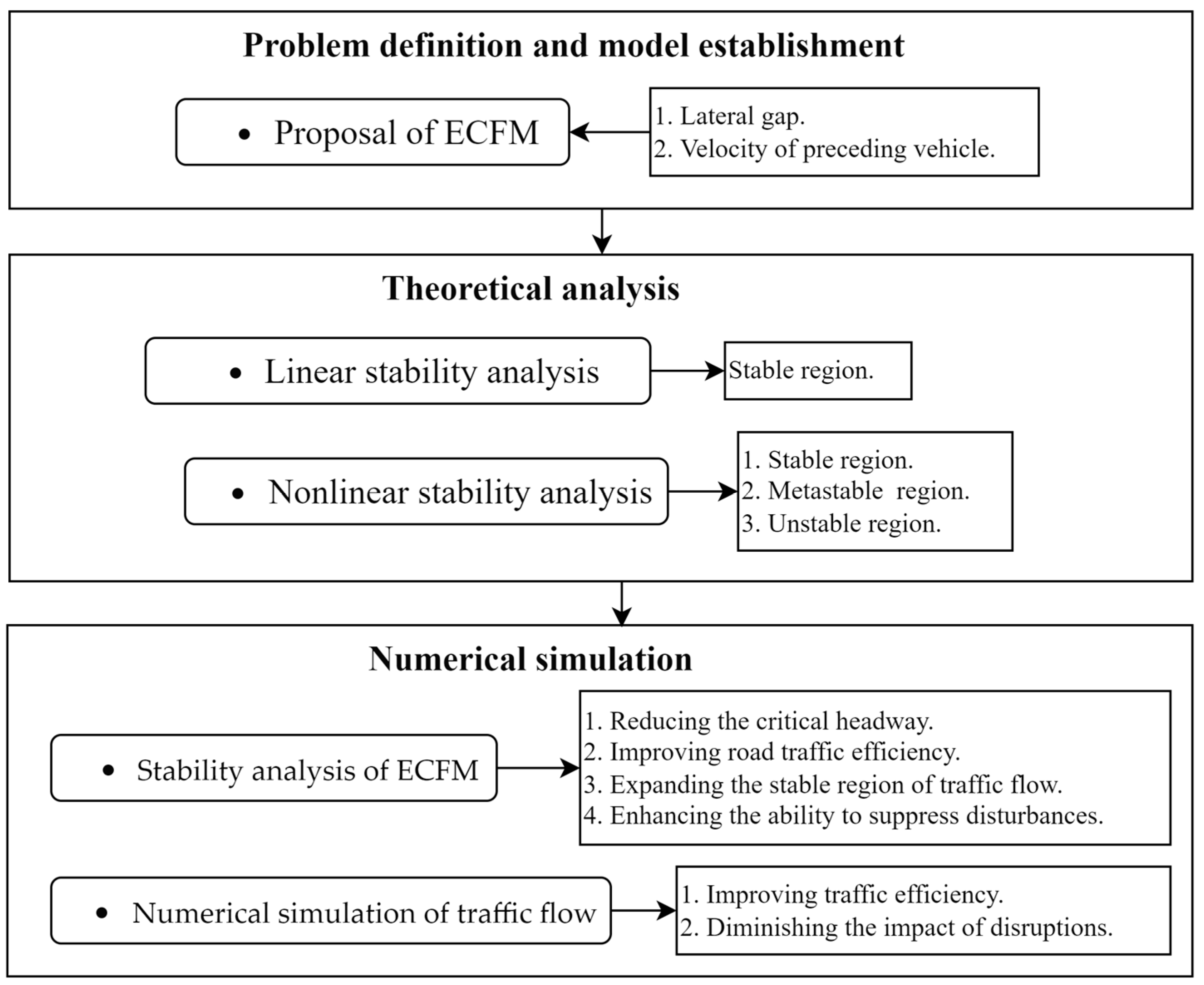
To develop a traffic model that better withstands disturbances and enhances the overall traffic efficiency, with significant implications for autonomous vehicle technology, it is essential to focus on creating an ECFM that more accurately predicts vehicle dynamics and improves traffic flow stability. This study assumes that the ITS acquires information on the lateral gap, optimal velocity, and velocity difference with respect to the preceding vehicle. It introduces the ratio of the lateral gap to lane width as a determinant for the car-following weight of the preceding vehicle. Subsequently, this study incorporates a car-following coefficient based on the optimal velocity of the preceding vehicle into the CFM and proposes an ECFM that simultaneously accounts for both lateral gap and optimal velocity. The stability conditions of the model are obtained by employing linear and nonlinear stability analyses. Here, the triangular shock wave in the stable region is solved using the Burgers equation. The kink–antikink wave in the metastable region is solved using the modified Korteweg–de Vries (mKdV) equation, and the solitary wave in the unstable region is solved using the Korteweg–de Vries (KdV) equation. Finally, the effectiveness of the proposed ECFM is verified through simulations conducted under periodic boundary conditions. The results demonstrate that the proposed ECFM can effectively enhance both the anti-interference capability and the size of the stable region of traffic flow. The research flow of this study is outlined in Figure 1, providing a visual representation of the various stages of the investigation. The main contributions of this research can be summarized as follows:
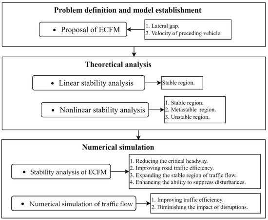
Figure 1.
Research flow.
- (1)
- Integrated Car-Following Weight: introducing the ratio of lateral gap to lane width as a car-following weight enhances realism and facilitates adaptive headway adjustments.
- (2)
- Expanded FVD Model: incorporating both lateral gap and optimal velocity of the preceding vehicle into the FVD model reduces the critical headway, expands the stable region, and improves traffic flow stability and efficiency.
- (3)
- Cumulative Enhancement: simultaneously considering lateral gap and optimal velocity synergistically enhances the traffic flow resistance to interference, reduces disruptions, and boosts the overall traffic efficiency.
2. Proposal of the ECFM
The FVD model accurately describes the car-following behavior, as shown below [31]:
where an (t) represents the acceleration of vehicle n at time t; κ and λ are the sensitivity parameters for optimal velocity and relative velocity, with κ = 1/τ, and τ being the driver’s reaction time; and Δxn (t) = xn+1 (t) − xn (t) and Δvn(t) = vn+1 (t) − vn (t) represent the headway and the relative velocity between vehicle n and vehicle n + 1 at time t, respectively. V(∆x) is the optimal velocity function, expressed as follows:
where hs is the safety distance, and vmax is the maximum velocity.
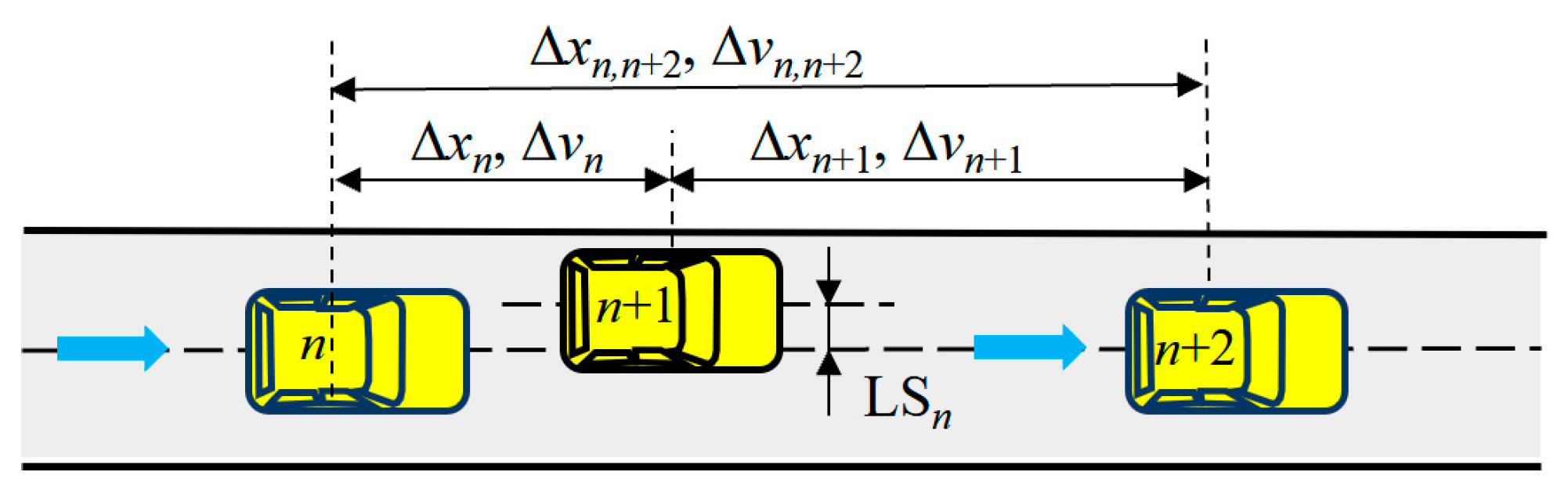
The FVD model assumes that all vehicles travel along the centerline of the lane, but vehicles are laterally positioned within the lane, following a normal distribution [15]. This phenomenon results in a lateral gap between the following vehicle and the preceding vehicle, which increases as the lane widens, as depicted in Figure 2. To address this issue, the FVD model was modified as follows [17]:
where V1 (·) and G (·) are expressed as follows:
where Δxn,n+2 (t) = xn+2 (t) − xn (t) and Δvn,n+2 (t) = vn+2 (t) − vn (t) represent the headway and the relative velocity between vehicle n and vehicle n + 2 at time t, respectively. p1 is the influencing parameter for the lateral gap of the preceding vehicle, defined as the following weight. In this study, p1 is defined as a variable rather than as a constant [32] and is represented as follows:
where LSn represents the lateral gap between vehicle n and vehicle n + 1, while LSmax represents the maximum lateral gap where the preceding vehicle has no influence on the following vehicle, and in this study, LSmax is set to the lane width of 3.6 m.
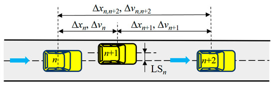
Figure 2.
A vehicle deviating from the centerline while following another vehicle.
Considering the lateral gap, this study proposes an ECFM that simultaneously considers the lateral gap and the optimal velocity of the preceding vehicle. The motion of the following vehicle is described as a function of the lateral gap and the optimal velocity between the following vehicle and the preceding vehicle. The expression for the acceleration of the following vehicle is as follows:
where p2 represents the weight coefficient of the optimal velocity of the preceding vehicle, with 0 ≤ p2 ≤ 1. It quantifies the extent to which the optimal velocity of the preceding vehicle n + 1 influences the current vehicle n. When p2 = 0, the optimal velocity of the preceding vehicle n + 2 has no impact on the optimal velocity of vehicle n. Conversely, when p2 = 1, the optimal velocity of the preceding vehicle n + 2 fully determines the optimal velocity of the current vehicle n. It should be noted that when a vehicle follows a vehicle in front, the lateral lag with respect to the front vehicle is generally not too large; therefore, p2 ≤ 0.2. Δxn+1(t) = xn+2 (t) − xn+1 (t) denotes the headway between vehicle n + 1 and vehicle n + 2 at time t.
The parameter p1 is used to describe the influence of the lateral gap. According to Equation (7), vehicle n follows both vehicle n + 1 and vehicle n + 2. When LSn is equal to zero, that is, p1 = 0, there is no lateral gap between vehicle n and vehicle n + 1. When LSn = LSmax, that is, p1 = 1, vehicle n + 1 is in another lane and has no impact on vehicle n. p2 quantifies the extent to which the optimal velocities of the two vehicles ahead, namely, vehicles n + 1 and n + 2, affect the current vehicle n. This parameter is crucial for simulating the real driving behavior, as it allows the trailing vehicle to adjust its velocity according to the optimal vehicles of multiple vehicles, rather than of just the one directly in front. This extended predictive capability is particularly useful in dense traffic situations or autonomous driving environments, where a smooth traffic flow and the reduction of sudden velocity changes are critical.
3. Linear Stability Analysis
Linear stability analysis is essential for determining the stability conditions of traffic flow under small disturbances, identifying stable regions, and understanding the propagation characteristics of perturbations. These insights help in designing more stable traffic control strategies. When a small perturbation is applied to a vehicle within a stable traffic flow, its motion states, such as acceleration and velocity, undergo abrupt changes. These changes also affect the headway and velocity differences between the vehicle and those ahead and behind it, ultimately disrupting the stable state of the traffic flow. This disturbance generates a perturbation wave that propagates backward. If this perturbation wave diminishes or disappears during its propagation, allowing the traffic flow to quickly stabilize or fluctuate slightly near the steady state, the traffic flow is considered stable. A linear stability analysis was performed on the model to obtain the stability conditions and evaluate the expanded effect of the proposed ECFM on the stable region. In this section, the perturbation method was employed to conduct a linear stability analysis on the ECFM. Equation (7) was rewritten as follows:
Assuming a stable traffic flow, the vehicles within the flow maintain the same headway and velocity. The velocity of vehicles in a stable traffic flow is given by:
where .
In a stable traffic flow, the distance of a vehicle relative to its initial position is given by:
Applying a small perturbation yn (t) to , the vehicle position relationship becomes:
The representation of the other vehicle states is as follows:
Substituting Equations (11)−(16) into Equation (9) and linearizing the resulting equation, we obtain:
where , .
In the Fourier mode, yn (t) can be expressed as e(ikn+zt). Therefore, we have:
By substituting Equations (18) and (19) into Equation (17), we obtain:
Let z = z1 (ik) + z2 (ik)2 + …, considering only the first two terms. Using the Taylor series to expand eik, i.e., eik = 1 + ik + 0.5(ik)2 + …, Equation (20) can be rewritten as:
Rearranging the equation as a polynomial in terms of ik, the coefficients of the first-order term and the second-order term are:
The above equation can be further rewritten as:
Setting z2 = 0, we can obtain the neutral stability condition as follows:
where , .
The condition that ensures the stability of the traffic flow against longer-wavelength disturbances is:
If the aforementioned conditions are met, then the traffic flow can return to a stable state after being perturbed. The larger the stable region, the stronger the disturbance resistance of the CFM. Conversely, if the perturbation does not dissipate in a timely manner and continues to propagate backward, it will ultimately cause the traffic flow to lose stability.
4. Nonlinear Stability Analysis
Nonlinear stability analysis delves into traffic flow behavior under large disturbances or nonlinear conditions, describing phenomena such as traffic jams, solitary waves, and density waves. It also helps validate the linear analysis results and provides practical guidance for managing large-scale traffic disruptions. Vehicle traffic flow is prone to forming density waves, leading to traffic congestion when subjected to disturbances. To analyze the nonlinear characteristics of the proposed ECFM, in this section, we utilized the reduced perturbation method to derive different nonlinear density wave equations and investigate the evolution mechanisms of stable, metastable, and unstable traffic flows [33,34]. The stable region refers to the conditions under which the traffic flow remains stable even when subjected to small disturbances. In this region, any perturbations will gradually dissipate, allowing the traffic flow to return to its steady state without forming traffic jams or other disruptions. The metastable region describes conditions where the traffic flow appears stable under small disturbances but can transition to an unstable state when subjected to larger perturbations. In this region, minor fluctuations can be absorbed without significant impact, but larger disruptions can trigger persistent traffic congestion. The unstable region indicates conditions where the traffic flow is inherently unstable, and any disturbance, whether small or large, will grow over time, leading to traffic jams and severe disruptions. In this region, the traffic flow cannot maintain a steady state, and instability is inevitable. These regions collectively describe the varying degrees of stability in traffic flow, with the stable region representing robust stability, the metastable region indicating conditional stability, and the unstable region signifying inherent instability.
For the convenience of subsequent calculations, Equation (7) was rewritten as follows:
4.1. Burgers Equation for the Stable Region
Deriving the Burgers equation for the stable region facilitates the description of the spatiotemporal evolution mechanism of small perturbations using the equation’s solutions. Introducing the slow variables X and T with respect to the spatial variable n and the temporal variable t:
where ε is a perturbation parameter, with 0 < ε ≪ 1, and b is a scaling constant used to scale the spatial variable and the temporal variable.
Let the headway be defined as:
Therefore,
Consequently,
Substituting Equations (27)–(30) into Equation (26) and expanding ε in a third-order Taylor series, we obtain the following nonlinear partial differential equation:
where , , , , .
Letting b = c1 and eliminating the second-order term of ε, simplifying Equation (31) yields the following:
Under the stability condition, the second-order partial derivative coefficient in Equation (31) is positive, that is:
In this case, Equation (32) is a Burgers equation, and one of its solutions is:
where , ηn represents the slope parameter along the X-axis, and ξn represents the coordinate of the front of the shock wave. c1 is the propagation speed of the triangular shock wave in the backward direction.
Equation (34) describes the propagation of a perturbation wave within the stable region following a disturbance in an initially stable traffic flow. As T → ∞, R(X,T) → 0, any density wave in a stable traffic flow will eventually evolve into a uniform and smooth traffic flow. A stable traffic flow can be described as vehicles traveling in a formation where both vehicle velocity and headway are the same.
4.2. KdV Equation for the Metastable Region
When deriving the KdV equation for the metastable region, we substitute Equations (27) and (28) into Equation (26) and expand ε in a sixth-order Taylor series. This process yields the following nonlinear partial differential equation:
where , .
The coefficients for the other terms are shown in Table 1.

Table 1.
Coefficients (ci) of the model.
Let b = c1. Near the neutral stability curve τ = (1 − ε2)τc, where τc = (2c1(c1 − λ(1 + p1)))/c2, by eliminating the third- and fourth-order terms of ε, Equation (35) can be simplified to:
The coefficients in the equation are shown in Table 2.
Table 2.
Coefficients (mi) of the model.
To obtain the standard KdV equation with higher-order remainder terms, the following transformation is applied to Equation (36):
From Equation (37), we can obtain:
Substituting Equation (38) into Equation (36) and simplifying, we obtain:
where .
Equation (39) is the KdV equation with a correction term of ο(ε). When the correction term ο(ε) is neglected, the solitary wave solution of the standard KdV equation is given by:
where A represents the amplitude of the solitary wave solution of the KdV equation.
Assuming that Rk (Xk,Tk)= Rk0 (Xk,Tk) + εRk1 (Xk,Tk), in order to determine the value of the parameter A, it is necessary to satisfy the solvability condition [34,35]
By evaluating the integral value of Equation (41), we obtain A as:
Thus, the headway expressed by the solitary wave solution is obtained as follows:
Through the derivation, we obtain the KdV equation near the neutral stability curve, which describes the propagation of a perturbation wave within the metastable region after an initially stable traffic flow is disturbed. This equation is used to describe the formation of solitary density waves in the traffic flow evolution and capture the “stop-and-go” driving phenomenon of vehicles within congested traffic.
4.3. mKdV Equation in the Unstable Region
We studied the slow variations in the spatial variable n and the temporal variable t of Equation (26) near the critical point (hc,τc) in the unstable region, where τc represents the critical sensitivity, and hc denotes the critical headway. When the slow variables X and T are defined as in Equation (27), the headway between vehicle n and vehicle n + 1 can be expressed as:
Substituting Equations (27) and (45) into Equation (26) and expanding it in a Taylor series up to the fifth order with respect to ε, we obtain the following nonlinear partial differential equation:
Let , . Here, , and in c1 and c2. When approaching the vicinity of the critical point (hc, ac), by eliminating the quadratic and cubic terms of ε, Equation (45) can be simplified to:
The coefficients in the equation are shown in Table 3.
Table 3.
Coefficients (ki) of the model.
The transformation applied to Equation (46) is as follows:
The resulting standard mKdV equation, including the correction term, is obtained as follows:
where .
By neglecting the correction term ο(ε), we obtain the kink–antikink density wave solution of the standard mKdV equation as:
Similar to the process of deriving the amplitude A of the KdV equation in Section 4.2, we can obtain the propagation velocity of the kink–antikink density wave solution as:
Therefore, the solution for the headway of the kink–antikink density wave is obtained as follows:
The amplitude C of the kink–antikink density wave is:
The solution of the kink–antikink density wave represents coexistent phases of the traffic flow, including free flow with low density and congested flow with high density, and represents the propagation of a perturbation wave within the unstable region after an initially stable traffic flow is disturbed. The headways in the free and congested flow are, respectively, given by ∆xn (t) = hc + C and ∆xn (t) = hc − C. This description captures the occurrence of kink–antikink density waves in the traffic flow evolution and characterizes the “stop-and-go” driving phenomenon of vehicles within congested traffic.
From ∆xn (t) = hc ± C, it can be inferred:
5. Stability Analysis of the ECFM
In this section, we analyze the stability of the proposed ECFM, an extension of the original FVD model, which does not consider lateral gaps and the optimal velocity of the preceding vehicle. Building on the established framework of the original FVD model, we introduce our enhancements. Instability in traffic flow occurs when small disturbances grow over time, leading to congestion and “stop-and-go” patterns, indicating that the flow cannot return to a steady state. Stability, on the other hand, implies that small disturbances dissipate, allowing the traffic to return to a steady state, resulting in a smooth and consistent flow. Metastability is an intermediate state where traffic can remain stable under small disturbances but may become unstable if disturbances exceed a certain threshold, causing oscillations between stable and unstable states. We used perturbation methods to conduct this stability analysis, determining the conditions under which the traffic flow remains stable. By linear stability analysis, we identified the thresholds for transitions between stable, metastable, and unstable regions. By nonlinear stability analysis, we further explored the traffic flow behavior under various perturbations, providing a comprehensive understanding of the model’s stability characteristics.
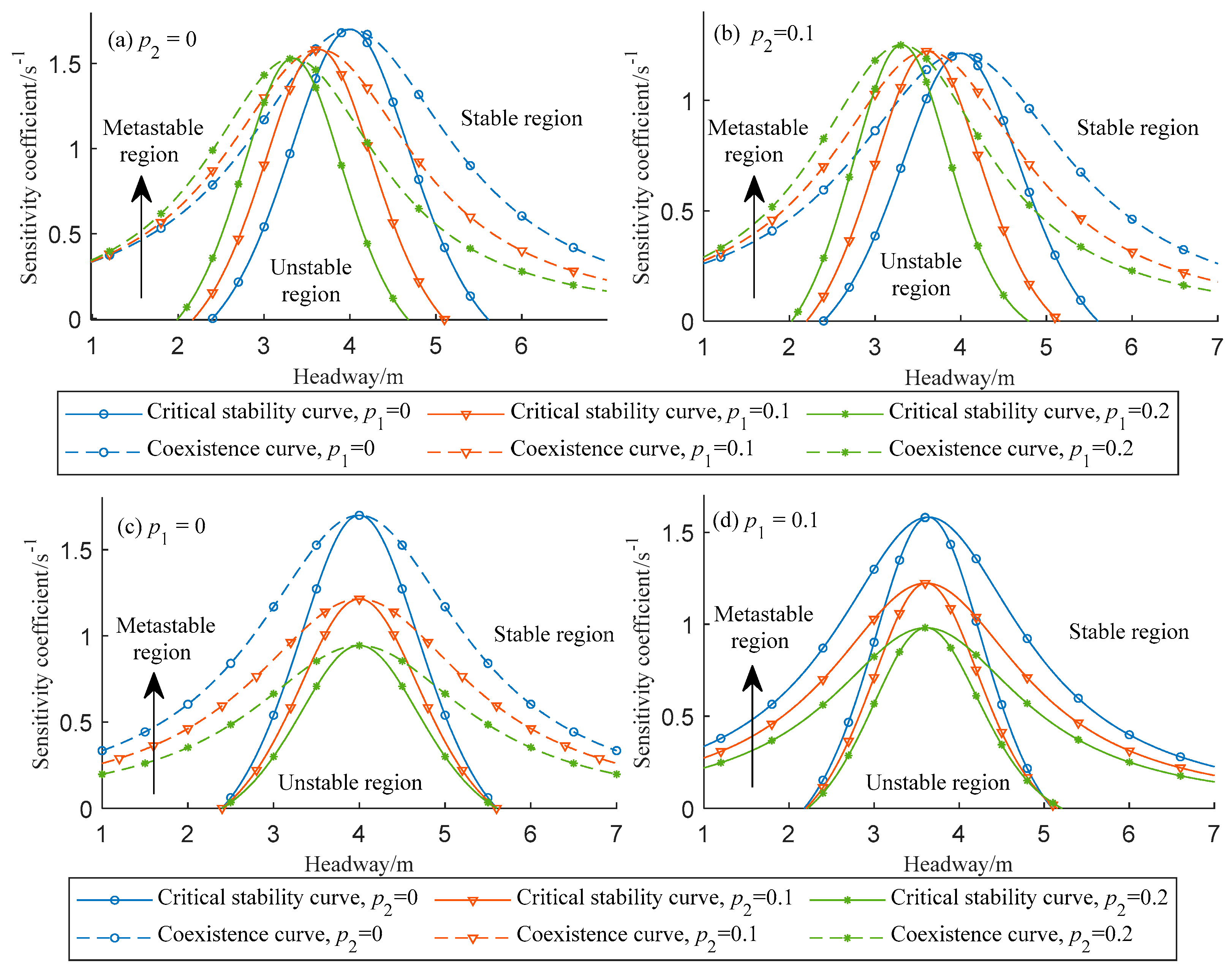
Figure 3 illustrates the critical stability curve (solid line) and coexistence curve (dashed line) under different values of p1 and p2 when λ = 0.15. The coexistence curve was determined by Equation (53). The region below the critical stability curve represents the unstable region, indicating that an initially stable traffic flow will lead to traffic congestion as it evolves with slight disturbances. The region above both the critical stability curve and the coexistence curve represents the stable region, indicating a free-flowing traffic phase. In the stable region, an initially stable traffic flow will dissipate disturbances as it evolves with slight perturbations. The other region is the metastable region, which indicates areas where the traffic flow can maintain temporary stability but is prone to losing stability when subjected to larger disturbances. When p1 = 0 and p2 = 0, the ECFM model degenerates into the FVD model.
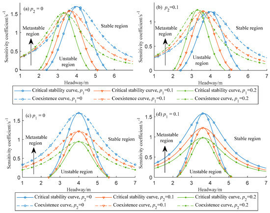
Figure 3.
Comparison of traffic flow stability under different values of p1 and p2.
From Figure 3, it can be observed that the parameters p1 and p2 have a significant impact on the stable region of the ECFM, as follows:
- (1)
- In Figure 3a, when p2 = 0, the critical stability curve shifts to the left as p1 increases from 0 to 0.1 and 0.2. This phenomenon indicates that a larger lateral gap results in a smaller critical headway, leading to improved traffic efficiency. Additionally, the critical stability curve moves downward, resulting in a reduction in the unstable region area by 15.32% and 26.62%, respectively, compared to p1 = 0. Thus, introducing a lateral gap in the FVD model decreases the critical headway and expands the stable region, improving road traffic efficiency and enhancing traffic flow stability, effectively reducing the occurrence of traffic congestion.
- (2)
- In Figure 3b, when p2 = 0.1, the critical headway decreases, and the unstable region area reduces by 9.40% and 16.24% as p1 increases from 0 to 0.1 and 0.2, respectively. Considering the lateral gap under the premise of a certain influence of the optimal velocity of the preceding vehicle will expand the stable region of traffic flow.
- (3)
- In Figure 3c, when p1 = 0, increasing p2 from 0 to 0.1 and 0.2 does not change the critical headway. However, both the critical stability curve and the coexistence curve decrease significantly. The unstable region area decreases by 28.57% and 44.44% compared to p2 = 0, indicating that introducing the optimal velocity of the preceding vehicle in the FVD model also expands the stable region and enhances the traffic flow stability.
- (4)
- In Figure 3d, when p1 = 0.1, increasing p2 from 0 to 0.1 and 0.2 results in a downward shift of the critical stability curve, and the unstable region area decreases by 23.05% and 38.07% compared to p2 = 0. Compared to the cases of p1 = 0 and p2 = 0, the unstable region area decreases by 34.82% when p1 = 0.1 and p2 = 0.1.
In summary, considering either the lateral gap of the preceding vehicle or the optimal velocity of the preceding vehicle in the CFM improves the stability and efficiency of the traffic flow, expanding the stable region of the CFM. Simultaneously considering both the lateral gap and the optimal velocity of the preceding vehicle in the CFM results in cumulative enhancement effects. Therefore, the proposed ECFM not only reduces the critical headway and improves road traffic efficiency but also expands the stable region of the traffic flow, enhancing the ability to suppress disturbances. These advantages contribute to reducing harmful gas emissions and energy consumption, promoting the sustainable development of the environment.
6. Numerical Simulation of the Traffic Flow
In this section, periodic boundary conditions were adopted to describe the evolution of headways in the traffic flow after being perturbed using the ECFM. The objective was to verify the inhibitory effect of considering the lateral gap and optimal velocity of the preceding vehicle on perturbations. As in the analysis in Section 4, when p1 = 0 and p2 = 0, the ECFM model was reduced to the FVD model. The advantages of the ECFM improvements can be clearly observed by comparing the results.
It was assumed that there were N vehicles distributed on the lane, and the front-to-following vehicle gaps were fixed. The initial conditions were as follows [17]:
When n ≠ 0.5N and n ≠ 0.5N +1:
When n = 0.5N +1:
When n = 0.5N:
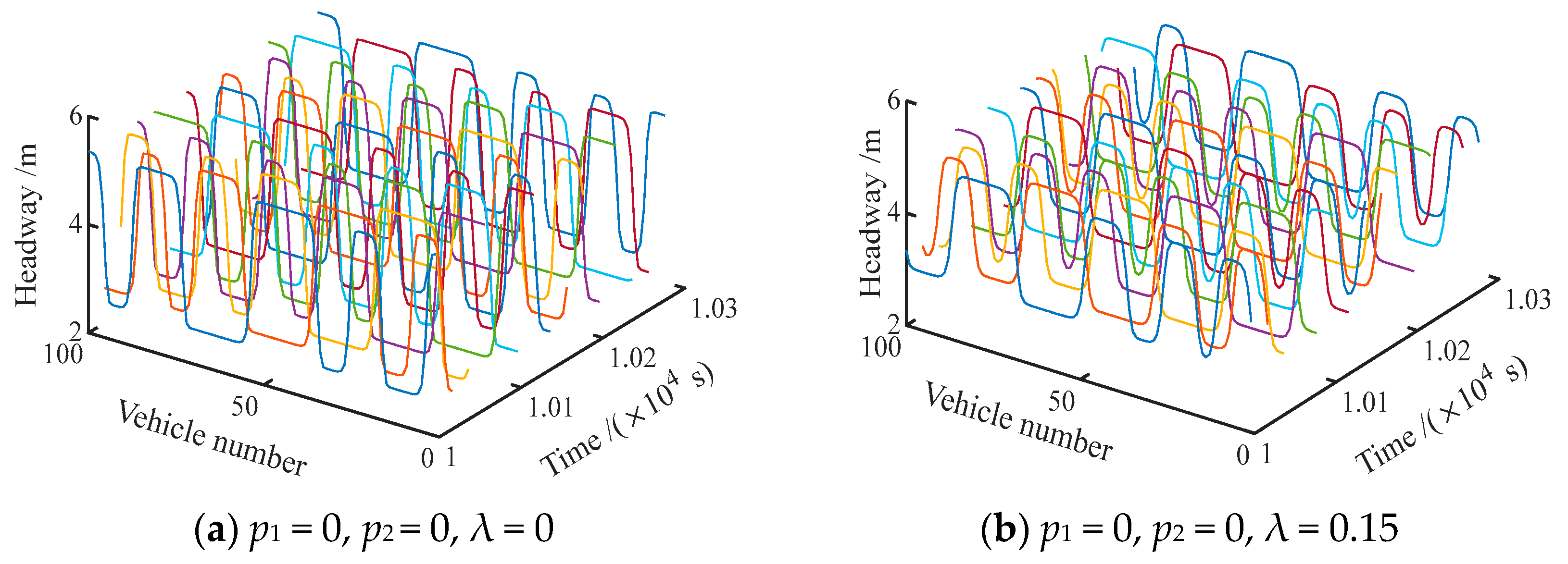
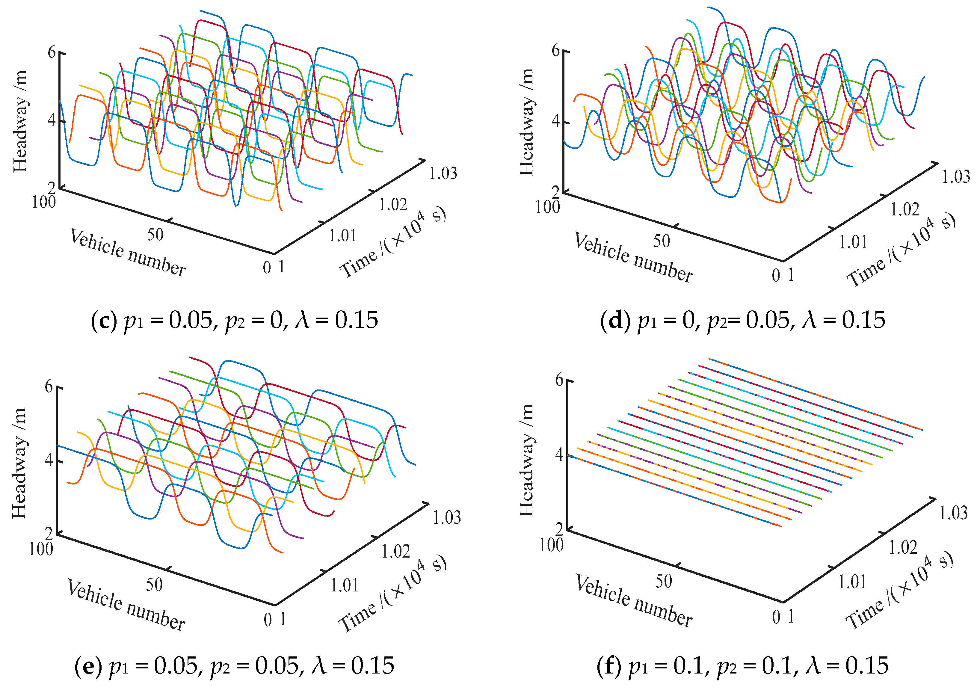
The remaining unspecified parameters of the model were set as follows: κ = 1.2 s−1, vmax = 2.0 m/s, N = 100, and hc = 4 m. To reflect the influence of the lateral gap and optimal velocity of the preceding vehicle on traffic flow evolution, an analysis was conducted on how parameter variations affect the headway in traffic flow. To ensure that the analyzed traffic flow had sufficiently evolved, the headway evolution data after 10,000 s of numerical simulation were provided, as shown in Figure 4. In this figure, the “vehicle number” refers to the index of the vehicle participating in the simulation, i.e., the nth vehicle. According to the stability condition (27), the traffic flow is stable only when p1 = 0.1, p2 = 0.1, and λ = 0.15. For the remaining five sets of parameter conditions in Figure 4, the traffic flow is in an unstable state. Therefore, only when p1 = 0.1, p2 = 0.1, and λ = 0.15, small perturbations will gradually disappear over time, while perturbations under other conditions will gradually evolve into traffic congestion.
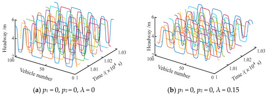

Figure 4.
Headway evolution.
The standard deviation reflects the dispersion of a dataset. In this study, the standard deviation of the headway in a simulation time from 10,000 s to 10,300 s was used to represent the dispersion in the numerical simulations. Headway dispersion is crucial for assessing traffic stability and smoothness; a lower dispersion indicates a more stable traffic flow, with reduced congestion and enhanced overall traffic efficiency. Table 4 presents the headway dispersion under different values of p1, p2, and λ. Combining the analyses of Table 4 and Figure 4, the following observations can be made:
Table 4.
Headway dispersion under different parameters.
- (1)
- From Figure 4a,b, it can be observed that when p1 = 0, p2 = 0, and λ = 0 or λ = 0.15, a small disturbance applied to a stable traffic flow amplifies as the traffic flow evolves, leading to vehicle congestion. When λ = 0, the traffic flow is in an unstable state and prone to congestion. However, with an increase in λ to 0.15 and considering the velocity difference, the headway dispersion in the traffic flow decreases by 30.99% compared to Figure 4a, indicating an improvement in the stability of the traffic flow.
- (2)
- From Figure 4c,d, it can be observed that when p1 = 0.05, p2 = 0 or p1 = 0, and p2 = 0.05, the same disturbance in the traffic flow amplifies during traffic evolution, resulting in traffic congestion. The headway dispersion in the traffic flow decreases by 8.29% and 47.92% compared to Figure 4b, respectively, when considering only the lateral gap or the optimal velocity of the preceding vehicle. This indicates that considering only the lateral gap or the optimal velocity of the preceding vehicle can suppress disturbances but not eliminate their effects completely.
- (3)
- From Figure 4e, when p1 = 0.05 and p2 = 0.05, simultaneously considering the lateral gap and the optimal velocity of the preceding vehicle, the headway dispersion in the traffic flow decreases by 94.63% and 90.55% compared to Figure 4c,d, respectively. This indicates that simultaneously considering the lateral gap and the optimal velocity of the preceding vehicle can further improve traffic congestion. The proposed model in this study outperforms the CFM considering only the lateral gap proposed in reference [17].
- (4)
- From Figure 4f, when p1 = 0.1 and p2 = 0.1, the disturbance does not evolve into traffic congestion but completely disappears as the traffic flow tends to a stable state. This indicates that increasing the following weight and the coefficient of optimal velocity of the preceding vehicle can prevent disturbances from spreading in the traffic flow.
In summary, simultaneously considering the lateral gap and the optimal velocity of the preceding vehicle can effectively enhance the anti-interference capability of the traffic flow, suppress the impact of disturbances, and improve traffic efficiency.
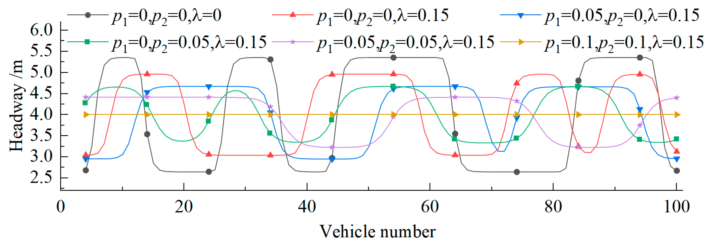
Figure 5 shows the headway distribution influenced by different values of p1, p2, and λ at t = 10,300 s for the ECFM. From the figure, it can be observed that as λ increases while p1 and p2 are fixed, the headway variation decreases, indicating an increased ability of the traffic flow to suppress congestion. When p2 and λ are fixed, increasing p1, that is, increasing the following weight, leads to a reduced variation in the headway when the traffic flow is disturbed. As the traffic flow evolves, the impact of disturbances on the traffic flow decreases. Similarly, when p1 and λ are fixed, increasing p2, that is, increasing the coefficient of optimal velocity for the following car, gradually reduces the headway variation when the traffic flow is disturbed, indicating that the lateral gap and the optimal velocity of the preceding vehicle promote the stability of the traffic flow. Investigations into headway profiles indicate that concomitantly considering both the lateral gap and the optimal velocity of the leading vehicle significantly enhances the traffic flow’s ability to resist interference. This method not only improves traffic efficiency but also diminishes the impact of disruptions. Collectively, these results corroborate the superior performance of the proposed ECFM, in alignment with the findings depicted in Figure 4.
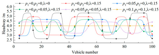
Figure 5.
Headway profile.
7. Conclusions
This study introduces an ECFM that simultaneously considers the lateral gap and the optimal velocity of the preceding vehicle. The model was subjected to both linear stability and nonlinear analyses, and stability conditions were derived. The theoretical analysis of linear stability revealed that considering the optimal velocity of the preceding vehicle, in addition to the lateral gap, further expanded the stable region of traffic flow, thereby reducing the probability of congestion. A nonlinear analysis was conducted using the perturbation method, and the numerical simulation results demonstrated that considering both the lateral gap and the optimal velocity of the preceding vehicle, compared to considering only the lateral gap as in the CFM, effectively enhanced the anti-interference capability of the traffic flow, suppressed the impact of disturbances, and improved traffic efficiency. The mutual validation between the theoretical analysis and the numerical simulation confirmed the effectiveness, rationality, and superiority of the proposed ECFM. The advantages of the ECFM in ITSs include reducing traffic accidents, minimizing the injury and fatality rates, and lowering the associated societal and economic costs. In intelligent vehicles, it reduces the likelihood of accidents caused by sudden braking or lane changes, thereby enhancing driving comfort and safety.
Author Contributions
Conceptualization and funding acquisition, Z.Z.; formal analysis and investigation, W.F.; writing—original draft preparation, W.T. and Z.L.; writing—review and editing, C.H. All authors have read and agreed to the published version of the manuscript.
Funding
This project was sponsored by the Hunan Provincial Natural Science Foundation of China under Grant 2022JJ50020 and the Scientific Research Fund of Hunan Provincial Education Department under Grant 20A018.
Institutional Review Board Statement
Not applicable.
Informed Consent Statement
Not applicable.
Data Availability Statement
Data are contained within the article.
Conflicts of Interest
Author Wenming Feng was employed by Hengyang Tellhow Communication Vehicles Co., Ltd. The remaining authors declare that the research was conducted in the absence of any commercial or financial relationships that could be construed as a potential conflict of interest.
Notations
| Symbol | Description |
| n | Vehicle index |
| t | Time |
| an | Acceleration of vehicle n at time t |
| κ | Optimal velocity sensitivity |
| λ | Relative velocity sensitivity |
| τ | Driver reaction time |
| ∆x | Headway between two vehicles |
| Δvn (t) | Relative velocity between two vehicles |
| vmax | Maximum vehicle velocity |
| V(∙) | Optimal velocity function |
| hs | Safety distance |
| vmax | Maximum velocity |
| p1 | Influencing coefficient of lateral gap |
| p2 | Weight coefficient |
| LS | Lateral gap between two vehicles |
| LSmax | Maximum lateral gap |
| c1 | First stability coefficient |
| c2 | Second stability coefficient |
| ε | Perturbation parameter |
| b | Scaling constant |
| m | Flow stability coefficient |
| ηn | Slope parameter |
| ξn | Coordinate of the front of the shock wave |
| τc | Critical sensitivity |
| hc | Critical headway |
| A | Amplitude of the solitary wave solution of the KdV equation |
| C | Amplitude of the kink–antikink density wave |
| c | Propagation velocity of the kink–antikink density wave solution |
| N | Number of vehicles |
References
- Liu, W.; Chen, Y.; Li, H.; Zhang, H. Quantitative study on road traffic environment complexity under car-following condition. Sustainability 2022, 14, 6251. [Google Scholar] [CrossRef]
- Sun, J.; Zheng, Z.; Sharma, A.; Sun, J. Stability and extension of a car-following model for human-driven connected vehicles. Transp. Res. Part C Emerg. Technol. 2023, 155, 104317. [Google Scholar] [CrossRef]
- Li, X.; Luo, X.; He, M.; Chen, S. An improved car-following model considering the influence of space gap to the response. Phys. A Stat. Mech. Its Appl. 2018, 509, 536–545. [Google Scholar] [CrossRef]
- Delpiano, R.; Herrera, J.C.; Laval, J.; Coeymans, J.E. A two-dimensional car-following model for two-dimensional traffic flow problems. Transp. Res. Part C Emerg. Technol. 2020, 114, 504–516. [Google Scholar] [CrossRef]
- Li, M.; Fan, J.; Lee, J. Modeling Car-Following Behavior with Different Acceptable Safety Levels. Sustainability 2023, 15, 6282. [Google Scholar] [CrossRef]
- Kuang, H.; Wang, M.T.; Lu, F.H.; Bai, K.Z.; Li, X.L. An extended car-following model considering multi-anticipative average velocity effect under V2V environment. Phys. A Stat. Mech. Its Appl. 2019, 527, 121268. [Google Scholar] [CrossRef]
- Sun, Y.; Ge, H.; Cheng, R. An extended car-following model under V2V communication environment and its delayed-feedback control. Phys. A Stat. Mech. Its Appl. 2018, 508, 349–358. [Google Scholar] [CrossRef]
- Zhu, W.X.; Zhang, H.M. Analysis of mixed traffic flow with human-driving and autonomous cars based on car-following model. Phys. A Stat. Mech. Its Appl. 2018, 496, 274–285. [Google Scholar] [CrossRef]
- Zong, F.; Wang, M.; Tang, J.; Zeng, M. Modeling AVs & RVs’ car-following behavior by considering impacts of multiple surrounding vehicles and driving characteristics. Phys. A Stat. Mech. Its Appl. 2022, 589, 126625. [Google Scholar]
- Ma, G.; Ma, M.; Liang, S.; Wang, Y.; Zhang, Y. An improved car-following model accounting for the time-delayed velocity difference and backward looking effect. Commun. Nonlinear Sci. Numer. Simul. 2020, 85, 105221. [Google Scholar] [CrossRef]
- Cao, B.G. A car-following dynamic model with headway memory and evolution trend. Phys. A Stat. Mech. Its Appl. 2020, 539, 122903. [Google Scholar] [CrossRef]
- Sun, Y.; Ge, H.; Cheng, R. An extended car-following model considering driver’s memory and average speed of preceding vehicles with control strategy. Phys. A Stat. Mech. Its Appl. 2019, 521, 752–761. [Google Scholar] [CrossRef]
- Zhai, C.; Wu, W. A new car-following model considering driver’s characteristics and traffic jerk. Nonlinear Dyn. 2018, 93, 2185–2199. [Google Scholar] [CrossRef]
- Li, Y.; Chen, B.; Zhao, H.; Peeta, S.; Hu, S.; Wang, Y.; Zheng, Z. A car-following model for connected and automated vehicles with heterogeneous time delays under fixed and switching communication topologies. IEEE Trans. Intell. Transp. 2021, 23, 14846–14858. [Google Scholar] [CrossRef]
- Noorvand, H.; Karnati, G.; Underwood, B.S. Autonomous vehicles: Assessment of the implications of truck positioning on flexible pavement performance and design. Transport. Res. Rec. 2017, 2640, 21–28. [Google Scholar] [CrossRef]
- Liu, D.W.; Shi, Z.K.; Ai, W.H. Modeling for Micro Traffic Flow with the Consideration of Lateral Vehicle’s Influence. J. Adv. Transport. 2021, 2020, 1–13. [Google Scholar] [CrossRef]
- Jin, S.; Wang, D.; Tao, P.; Li, P. Non-lane-based full velocity difference car following model. Phys. A Stat. Mech. Its Appl. 2010, 389, 4654–4662. [Google Scholar] [CrossRef]
- Hadadi, F.; Tehrani, H.G.; Aghayan, I. An extended non-lane-discipline-based continuum model through driver behaviors for analyzing multi-traffic flows. Phys. A Stat. Mech. Its Appl. 2023, 625, 128965. [Google Scholar] [CrossRef]
- Kashyap, N.R.M.; Chilukuri, B.R.; Srinivasan, K.K.; Asaithambi, G. Analysis of vehicle-following behavior in mixed traffic conditions using vehicle trajectory data. Transport. Res. Rec. 2020, 2674, 842–855. [Google Scholar] [CrossRef]
- Wen, X.; Jian, S.; He, D. Modeling the effects of autonomous vehicles on human driver car-following behaviors using inverse reinforcement learning. IEEE Trans. Intell. Transp. 2023, 24, 13903–13915. [Google Scholar] [CrossRef]
- Xue, Y.; Wang, L.; Yu, B.; Cui, S. A two-lane car-following model for connected vehicles under connected traffic environment. IEEE Trans. Intell. Transp. 2024, 25, 7445–7453. [Google Scholar] [CrossRef]
- Talal, M.; Ramli, K.N.; Zaidan, A.A.; Zaidan, B.B.; Jumaa, F. Review on car-following sensor based and data-generation mapping for safety and traffic management and road map toward ITS. Veh. Commun. 2020, 25, 100280. [Google Scholar] [CrossRef]
- Han, J.; Wang, X.; Wang, G. Modeling the car-following behavior with consideration of driver, vehicle, and environment factors: A historical review. Sustainability 2022, 14, 8179. [Google Scholar] [CrossRef]
- Wang, X.; Jerome, Z.; Wang, Z.; Zhang, C.; Shen, S.; Kumar, V.V.; Bai, F.; Krajewski, P.; Deneau, D.; Jawad, A.; et al. Traffic light optimization with low penetration rate vehicle trajectory data. Nat. Commun. 2024, 15, 1306. [Google Scholar] [CrossRef] [PubMed]
- Yadav, S.; Redhu, P. Impact of driving prediction on headway and velocity in car-following model under V2X environment. Phys. A Stat. Mech. Its Appl. 2024, 635, 129493. [Google Scholar] [CrossRef]
- Wang, Z.; Shi, Y.; Tong, W.; Gu, Z.; Cheng, Q. Car-following models for human-driven vehicles and autonomous vehicles: A systematic review. J. Transp. Eng. A-Syst. 2023, 149, 04023075. [Google Scholar] [CrossRef]
- Qu, D.; Wang, S.; Liu, H.; Meng, Y. A car-following model based on trajectory data for connected and automated vehicles to predict trajectory of human-driven vehicles. Sustainability 2022, 14, 7045. [Google Scholar] [CrossRef]
- Lin, D.C.; Li, L. An Efficient Safety-Oriented Car-Following Model for Connected Automated Vehicles Considering Discrete Signals. IEEE Trans. Veh. Technol. 2023, 72, 9783–9795. [Google Scholar] [CrossRef]
- Han, J.; Wang, X.; Shi, H.; Wang, B.; Wang, G.; Chen, L.; Wang, Q. Research on the impacts of vehicle type on car-following behavior, fuel consumption and exhaust emission in the V2X environment. Sustainability 2022, 14, 15231. [Google Scholar] [CrossRef]
- Peng, G.; Wang, K.; Zhao, H.; Tan, H. Integrating cyber-attacks on the continuous delay effect in coupled map car-following model under connected vehicles environment. Nonlinear Dyn. 2023, 111, 13089–13110. [Google Scholar] [CrossRef]
- Jiang, R.; Wu, Q.; Zhu, Z. Full velocity difference model for a car-following theory. Phys. Rev. E 2001, 64, 017101. [Google Scholar] [CrossRef] [PubMed]
- Li, Y.; Zhang, L.; Peeta, S.; Pan, H.; Zheng, T.; Li, Y.; He, X. Non-lane-discipline-based car-following model considering the effects of two-sided lateral gaps. Nonlinear Dyn. 2015, 80, 227–238. [Google Scholar] [CrossRef]
- Ma, G.; Li, K.; Sun, H. Modeling and simulation of traffic flow based on memory effect and driver characteristics. Chin. J. Phys. 2023, 81, 144–154. [Google Scholar] [CrossRef]
- Ma, M.; Ma, G.; Liang, S. Density waves in car-following model for autonomous vehicles with backward looking effect. Appl. Math. Model. 2021, 94, 1–12. [Google Scholar] [CrossRef]
- Hossain, M.A.; Tanimoto, J. A dynamical traffic flow model for a cognitive drivers’ sensitivity in Lagrangian scope. Sci. Rep. 2022, 12, 17341. [Google Scholar] [CrossRef]
Disclaimer/Publisher’s Note: The statements, opinions and data contained in all publications are solely those of the individual author(s) and contributor(s) and not of MDPI and/or the editor(s). MDPI and/or the editor(s) disclaim responsibility for any injury to people or property resulting from any ideas, methods, instructions or products referred to in the content. |
© 2024 by the authors. Licensee MDPI, Basel, Switzerland. This article is an open access article distributed under the terms and conditions of the Creative Commons Attribution (CC BY) license (https://creativecommons.org/licenses/by/4.0/).