Enhancing Sustainable Development: Assessing a Solar Air Heater (SAH) Test Bench through Computational and Experimental Methods

Abstract

A solar air heater is a device that gathers solar radiation and converts it into heat. The core principle involves air moving through a solar collector, where sunlight naturally increases the air temperature within the collector. The benefit of this technology lies in its affordability and simplicity. The implementation of a solar air heater (SAH) test bench holds significant promise in addressing both global change and sustainable development objectives. The primary goal of this study is to examine the aerodynamic configuration of a novel solar air heater test bench accessible at the Laboratory of Electro-Mechanic Systems (LASEM). This study was carried out using the standard k-ω turbulence model with the use of the ANSYS Fluent 17.0 software. The results indicate that the velocity at the inlet directly influences the velocity fields, temperature, static pressure, and characteristics of turbulence. Furthermore, the numerical findings confirmed that the temperature and velocity profiles in the second channel are in good concordance with the experimental findings in the case of a fan, placed alongside the insulation, operating in a delivery mode. Based on these results, the computational approach is validated. When comparingforced convection to natural convection under identical conditions, there was a notable increase in the energy efficiency, with forced convection showing a significant improvement of approximately 31.8%. Indeed, the range of temperatures reached with the proposed design, is highly beneficial for both industrial and household applications.

1. Introduction

Day-by-day, industries and societies are considering solar systems because of their eco-friendly nature with the use of renewable resources. The aim is to minimize energy consumption, so many researchers are working on this topic [1,2,3,4,5,6,7,8,9,10,11,12,13,14,15,16]. The deployment of SAH technology contributes to mitigating climate change by harnessing renewable energy sources, reducing the reliance on fossil fuels, and curbing greenhouse gas emissions. Additionally, SAH technology facilitates decentralized energy production, empowers communities to generate clean energy, and promotes energy independence. From a sustainable development perspective, SAH deployment fosters economic growth, creates job opportunities in the renewable energy sector, stimulates innovation in green technologies, and enhances energy access in off-grid and rural areas. Overall, the widespread adoption of SAH technology not only mitigates climate change but also fosters sustainable development by promoting clean energy, economic growth, and social well-being [1,2,3,4,5,6,7,8,9,10,11,12,13,14,15,16]. In this context, a distinction among the recorded temperatures at the outlet of moving air was made by El-Sebaii et al. [17]. Also, they presented the absorber plate temperatures and the output power of the SAH’s finned and corrugated surface. The outcome demonstrated that the SAH’s corrugated surface is about 9.3%. The optimal room temperature for forced circulation is 45.5 °C. For natural circulation, however, it is equal to 41.75 °C. Wazed et al. [18] engineered and constructed a SAH system which considered the context of a developing country with substantial energy requirements. The findings of this study confirm that its economical and uncomplicated technology makes it feasible in terms of cost, operation, and maintenance for the general populace of Bangladesh. Sopian et al. [19] established that incorporating a porous media into the double-pass (DP) enhances the quality of the collector. Then, the experimental validation of the theoretical model and its development showed that the theoretical and experimental data were well aligned. In addition, the quality of the porous media DP solar collector is around 60–70%. Esen [20] proposed an experimental study with and without barriers for a new flat plate SAH. The outcomes confirmed that the optimum performance value under all operating conditions is in the middle stage of the absorbing wall in the flow channel. Furthermore, the barriers-supplied double-flow collector appears substantially stronger than the one without barriers. A system device for inserting an aluminum absorbing wall into a flatplate SAH with a DP channel was experimentally investigated by Ozgen et al. [21]. Theodosius et al. [22] conducted comparisons using both numerical and experimental methods to elucidate the accuracy of the model. Han et al. [23] examined a combined solar energy setup. An overview of the designs for the structural envelope and the novel system was provided. Due to the importance of the SAH system, different designs have been studied. For example, Satcunana et al. [24] introduced the DP SAH concept and confirmed that a typical system demonstrated a higher efficiency than a single pass (SP). The efficiency of a DP SAH with numerous configurations of the absorber plate was the object of an inquiry conducted by Hassen et al. [25]. Conversely, on the basis of the findings of several experimental trials, Allam et al. [26] confirmed that the DP SAH has a better output than the SP one. As for the plate temperature in the DP heat exchanger, the findings of Goodarzi et al. [27] showed that it presents a greater temperature compared to the normal one. The power consumption for the handling of the flow rate is, in fact, higher than the one needed in the other considered cases. In relation to the other considered systems, Singh and Dhiman [28] proposed the application of the DP SAH to improve the thermal efficiency.

On the basis of these anterior study findings, the deployment of Solar Air Heater (SAH) technology represents a significant advancement over previous publications by directly harnessing renewable solar energy to heat air, thereby reducing the reliance on fossil fuels and curbing greenhouse gas emissions. Unlike the traditional heating methods documented in earlier studies, SAH systems offer sustainable heating solutions with lower operational costs and minimal environmental impacts. By leveraging innovative designs and materials, SAH technology achieves a higher thermal efficiency and contributes effectively to global efforts in mitigating climate change through the promotion of clean and renewable energy sources. The efficiency of SAH systems which employ a DP is recommended. Consequently, attention has been focused on examining a newly designed and laboratory-constructed SAH system with a double-pass. This study is particularly interested in conducting numerical simulations and experimental validations of the turbulent flow using the designated test setup.

2. Proposed SAH System

Figure 1a displays a recently utilized test bench for a SAH, which was created and assembled in the LASEM laboratory. This setup aims to assess the efficiency of a SAH comprising two channels divided by an absorber. It is equipped with a fan functioning in delivery mode, positioned at the inlet at the end of the insulation. The SAH system is attached to the prototype box by means of a pipe placed on the glass side and attached to the prototype by means of a duct. Then, in different heating applications, the outlet of the prototype box acts as an exhaust to vent hot air.

Figure 1b illustrates the geometric layout of the computational domain. It is divided into two sections by a duct with a diameter of 100 mm. The SAH has the dimensions of 194 mm in height and 778 mm in width. Attached to the front of the SAH is a glass panel measuring 1000 mm in length, and an absorber extending 1086 mm in length is placed inside it. Subsequently, the heated air is directed towards a box prototype measuring 1500 mm in length, 1100 mm in height, and 1000 mm in width. Also on the side of this prototype box are two circular openings which are positioned with a separation gap of 900 mm. These inlet holes, located at a height of 250 mm and a distance of 300 mm from the front, facilitate the entry of hot air, while an outlet hole permits its release into the surrounding environment.

All the symbols shown in Figure 1b are explained in

Table 1. Characteristics of the geometrical arrangements.

Parameters	Value (mm)
Length	1500
Height	1100
Width	1000
Longitude	300
Length	1086
Length	1000
Width 2	778
Height	194
Position 1	250
Position 2	900
Diameters	100

.

3. Computational Model

3.1. Mathematical Equations

At this point, the airflow is governed by equations in the Cartesian coordinate system [29].

The continuity equation is expressed as follows:

$$\frac{\partial \mathsf{\rho }}{\partial \mathrm{t}}+\frac{\partial }{\partial {\mathrm{x}}_{\mathrm{i}}}(\mathsf{\rho }{\mathrm{u}}_{\mathrm{i}})=0\hspace{0.17em}\hspace{0.17em}\hspace{0.17em}$$

(1)

The equations for momentum are formulated as follows:

$$\frac{\partial }{\partial \mathrm{t}}(\mathsf{\rho }{\mathrm{u}}_{\mathrm{i}})+\frac{\partial }{\partial {\mathrm{x}}_{\mathrm{j}}}(\mathsf{\rho }{\mathrm{u}}_{\mathrm{i}}\hspace{0.17em}{\mathrm{u}}_{\mathrm{j}})=-\frac{\partial \mathrm{p}}{\partial {\mathrm{x}}_{\mathrm{i}}}+\frac{\partial }{\partial {\mathrm{x}}_{\mathrm{i}}}\left[\mathsf{\mu }\left(\frac{\partial {\mathrm{u}}_{\mathrm{i}}}{\partial {\mathrm{x}}_{\mathrm{i}}}+\frac{\partial {\mathrm{u}}_{\mathrm{j}}}{\partial {\mathrm{x}}_{\mathrm{i}}}-\frac{2}{3}{\mathsf{\delta }}_{\mathrm{ij}}\hspace{0.17em}\frac{\partial {\mathrm{u}}_{\mathrm{i}}}{\partial {\mathrm{x}}_{\mathrm{i}}}\right)\right]+\frac{\partial }{\partial {\mathrm{x}}_{\mathrm{j}}}(-\mathsf{\rho }\overline{{\mathrm{u}}_{\mathrm{i}}^{\prime }{\mathrm{u}}_{\mathrm{j}}^{\prime }})+{\mathrm{F}}_{\mathrm{i}}$$

(2)

Then, the equations presented above are referenced to the Reynolds-averaged Navier–Stokes (RANS) equations. The terms $(-\rho \overline{u_i^{\prime }{u}_j^{\prime }})$ are defined to close the RANS equation:

$$(-\mathsf{\rho }\overline{{\mathrm{u}}_{\mathrm{i}}^{\prime }{\mathrm{u}}_{\mathrm{j}}^{\prime }})={\mathsf{\mu }}_{\mathrm{t}}\left(\frac{\partial {\mathrm{u}}_{\mathrm{i}}}{\partial {\mathrm{x}}_{\mathrm{j}}}+\frac{\partial {\mathrm{u}}_{\mathrm{j}}}{\partial {\mathrm{x}}_{\mathrm{i}}}\right)-\frac{2}{3}\left(\mathsf{\rho }\mathrm{k}+{\mathsf{\mu }}_{\mathrm{t}}\frac{\partial {\mathrm{u}}_{\mathrm{k}}}{\partial {\mathrm{x}}_{\mathrm{k}}}\right){\mathsf{\delta }}_{\mathrm{i}\mathrm{j}}$$

(3)

This method offers a lower computational expense relative to alternative numerical approaches. By utilizing the standard k-ω turbulence model, µ_t represents the turbulent viscosity determined by:

$${\mathsf{\mu }}_{\mathrm{t}}={\mathsf{\alpha }}^{\ast }\frac{\mathsf{\rho }\hspace{0.17em}\mathrm{k}}{\mathsf{\omega }}$$

(4)

α^∗ is calculated as follows:

$${\mathsf{\alpha }}^{\ast }={\mathsf{\alpha }}_{\infty }^{\ast }\left(\frac{{\mathsf{\alpha }}_0^{\ast }+\mathrm{R}{\mathrm{e}}_{\mathrm{t}}/{\mathrm{R}}_{\mathrm{k}}}{1+\mathrm{R}{\mathrm{e}}_{\mathrm{t}}/{\mathrm{R}}_{\mathrm{k}}}\right)$$

(5)

where:

$$\mathrm{R}{\mathrm{e}}_{\mathrm{t}}=\frac{\mathsf{\rho }\hspace{0.17em}\mathrm{k}}{\mathsf{\mu }\hspace{0.17em}\mathsf{\omega }}\hspace{0.17em}$$

(6)

$${\mathrm{R}}_{\mathrm{k}}=6$$

(7)

$${\mathsf{\alpha }}_0^{\ast }=\frac{{\mathsf{\beta }}_{\mathrm{i}}}{3}$$

(8)

$${\mathsf{\beta }}_{\mathrm{i}}=0.072$$

(9)

In case of the high-Reynolds number, α^∗ can be written as follows:

α^∗ = α^∗_∞ = 1

(10)

The turbulent kinetic energy k and the specific dissipation rate ω are described in this way:

$$\frac{\partial }{\partial \mathrm{t}}\left(\mathsf{\rho }\hspace{0.17em}\mathrm{k}\right)+\frac{\partial }{\partial {\mathrm{x}}_{\mathrm{i}}}\left(\mathsf{\rho }\hspace{0.17em}\mathrm{k}\hspace{0.17em}{\mathrm{u}}_{\mathrm{i}}\right)=\frac{\partial }{\partial {\mathrm{x}}_{\mathrm{i}}}\left({\Gamma }_{\mathsf{\omega }}\frac{\partial \mathrm{k}}{\partial {\mathrm{x}}_{\mathrm{j}}}\right)+{\mathrm{G}}_{\mathrm{k}}-{\mathrm{Y}}_{\mathrm{k}}+{\mathrm{S}}_{\mathrm{k}}$$

(11)

$$\frac{\partial }{\partial \mathrm{t}}\left(\mathsf{\rho }\hspace{0.17em}\mathsf{\omega }\right)+\frac{\partial }{\partial {\mathrm{x}}_{\mathrm{i}}}\left(\mathsf{\rho }\hspace{0.17em}\mathsf{\omega }\hspace{0.17em}{\mathrm{u}}_{\mathrm{i}}\right)=\frac{\partial }{\partial {\mathrm{x}}_{\mathrm{j}}}\left({\Gamma }_{\mathsf{\omega }}\frac{\partial \mathsf{\omega }}{\partial {\mathrm{x}}_{\mathrm{j}}}\right)+{\mathrm{G}}_{\mathsf{\omega }}-{\mathrm{Y}}_{\mathsf{\omega }}+{\mathrm{S}}_{\mathsf{\omega }}$$

(12)

Table 2. Constants of the k-ω model.

σω	σk	Rk	Rω	α∗∞	α∞	α0
2.0	2.0	6.0	2.95	1.0	1.9	1/9

displays the constants for the k-ω model.

The energy equation is written as follows:

$$\frac{\partial }{\partial \mathrm{t}}(\mathsf{\rho }\hspace{0.17em}\mathrm{E})+\frac{\partial }{\partial {\mathrm{x}}_{\mathrm{i}}}\left[{\mathrm{u}}_{\mathrm{i}}\left(\mathsf{\rho }\mathrm{E}+\mathrm{p}\right)\right]=\frac{\partial }{\partial {\mathrm{x}}_{\mathrm{j}}}\left[\left(\mathrm{K}+\frac{{\mathrm{c}}_{\mathrm{p}}{\mathsf{\mu }}_{\mathrm{t}}}{\mathrm{P}{\mathrm{r}}_{\mathrm{t}}}\right)\frac{\partial \mathrm{T}}{\partial {\mathrm{x}}_{\mathrm{j}}}+{\mathrm{u}}_{\mathrm{i}}{\left({\mathsf{\tau }}_{\mathrm{i}\mathrm{j}}\right)}_{\mathrm{e}\mathrm{f}\mathrm{f}}\right]+{\mathrm{S}}_{\mathrm{h}}$$

(13)

where ${\left({\mathsf{\tau }}_{\mathrm{i}\mathrm{j}}\right)}_{\mathrm{e}\mathrm{f}\mathrm{f}}$ is the stress tensor, defined as follows:

$${\left({\mathsf{\tau }}_{\mathrm{i}\mathrm{j}}\right)}_{\mathrm{e}\mathrm{f}\mathrm{f}}={\mathsf{\mu }}_{\mathrm{e}\mathrm{f}\mathrm{f}}\left(\frac{\partial {\mathrm{u}}_{\mathrm{j}}}{\partial {\mathrm{x}}_{\mathrm{i}}}+\frac{\partial {\mathrm{u}}_{\mathrm{i}}}{\partial {\mathrm{x}}_{\mathrm{j}}}\right)-\frac{2}{3}{\mathrm{\mu }}_{\mathrm{e}\mathrm{f}\mathrm{f}}\frac{\partial {\mathrm{u}}_{\mathrm{k}}}{\partial {\mathrm{x}}_{\mathrm{k}}}{\mathrm{\delta }}_{\mathrm{i}\mathrm{j}}$$

(14)

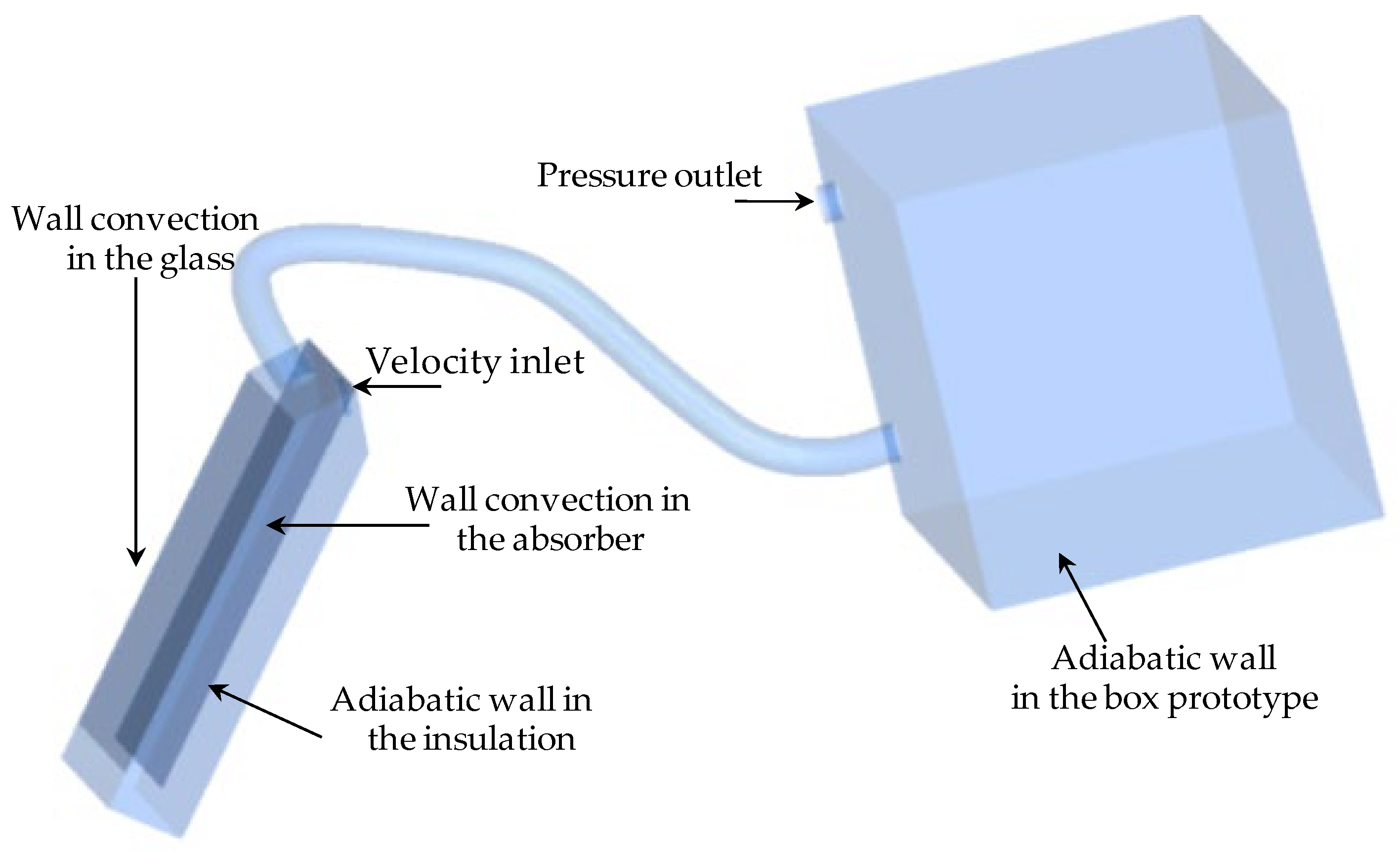
3.2. Boundary Conditions

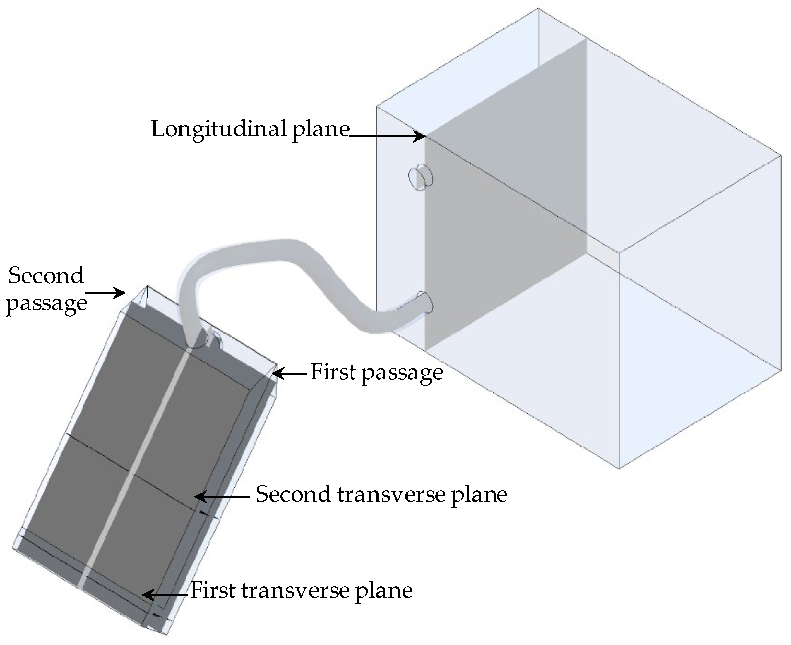
The boundary conditions are provided in Figure 2. At the inlet of the hole, a velocity of V = 3 m/s and a temperature of 308 K are specified. Conversely, the pressure at the outlet is established at P = 101,325 Pa, indicating that the fluid exits the system into an environment at atmospheric pressure. The inlet velocity of V = 3 m·s⁻¹ being considered corresponds to the range used in much more usual industrial applications like heating and drying [29].

The other values are based on the experimental test measurements. Indeed, a plate boundary was applied to the SAH test bench with a heat flux equal to zero in the lateral surface of the box prototype and the insulation planes, considered as adiabatic walls. A no-slip condition was used on the plates. For the absorber, considered as an opaque system, the coupled method was used for the thermal conditions. However, the convection used for the glass, considered as a semi-transparent plane, had a heat transmission coefficient equal to 8 W·m⁻²·K⁻¹. In these conditions, the direct irradiation is equal to 899.4 W·m⁻² and the diffuse irradiation is equal to 186.14 W·m⁻². Indeed, it has considered the discrete ordinates (DO) for the radiation model and the DO irradiation for the solar load. In fact, the computational cost is reasonable and the memory necessities are modest.

3.3. Meshing Choice

In this research, the SAH computational domain is discretized into a limited volume of unstructured pyramidal components. Then, the meshing options are considered and changed to obtain the results with a lower numerical diffusion (Figure 3). To perform the grid sensitivity tests, we have changed and tested the numbers of meshing cells. Four cases have been considered. The first mesh, corresponding to a coarse case is composed by 675,684 cells. The second mesh corresponds to 1,000,526 cells and the third mesh corresponds to 1,578,369 cells. However, the fourth mesh is more refined and corresponds to 1,865,129 cells. From these results, it has been noted that the numerical value of the average velocity, for the third and the fourth cases, present the same results with the experimental data. In these conditions, the gap is about 3.2%.

In addition, it was found that the resolution time increases with the decreasing size of the mesh. Thus, we adopt the model presenting an acceptable precision with a minimum resolution time. This study tends to show that the third meshing is more adequate to model the air flow in our prototype, as presented in Figure 4.

4. Results and Discussion

Figure 5 showcases the various visualization planes considered to study the distributions of velocity fields, temperature, radiation, pressure, kinetic energy, and dissipation rate. The Reynolds number is a dimensionless measure in fluid mechanics used to predict flow patterns in various fluid flow scenarios. It determines whether the flow will be laminar (smooth and orderly) or turbulent (chaotic and irregular). In this instance, the Reynolds number is calculated to be Re = 20,000.

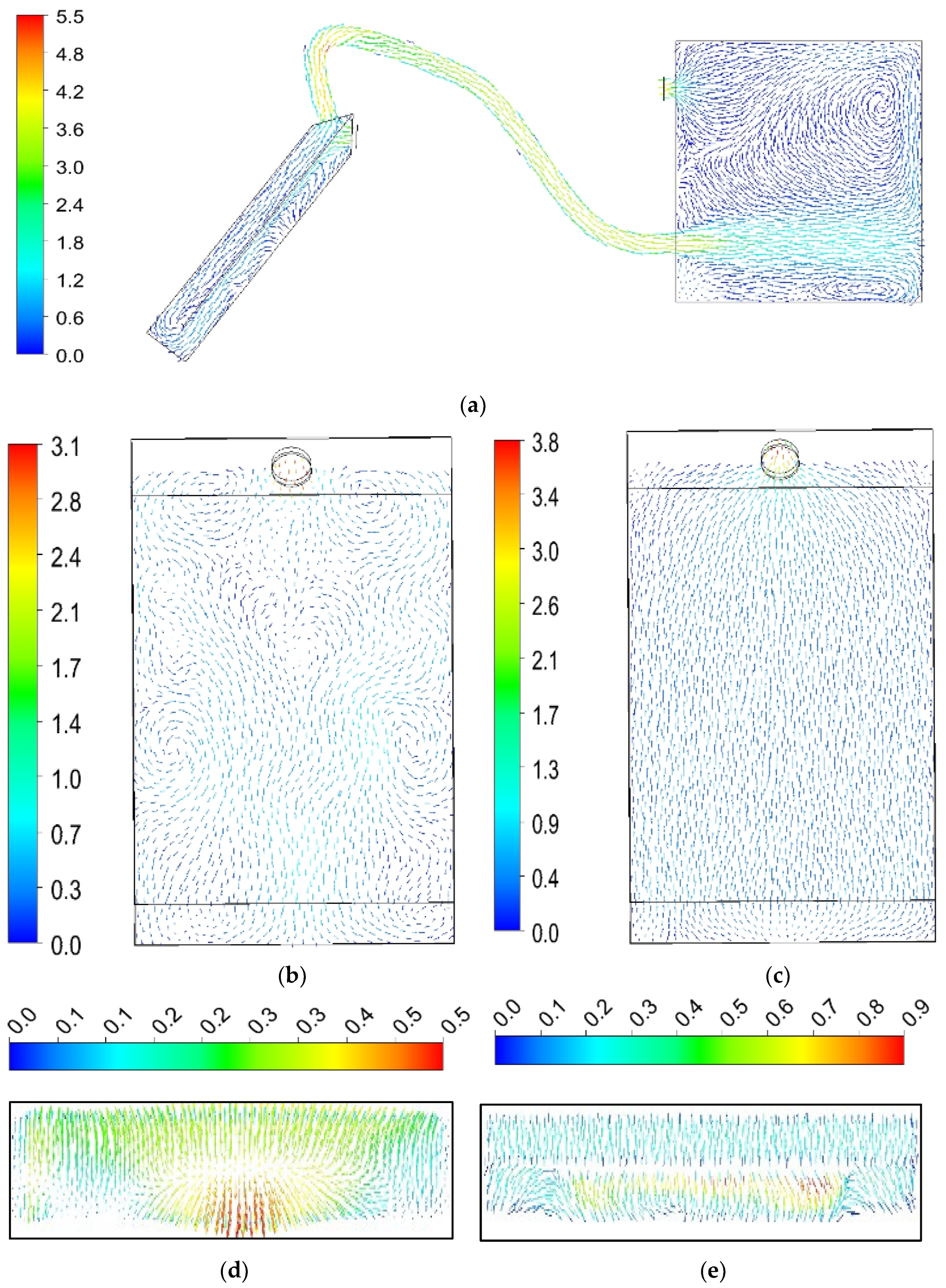
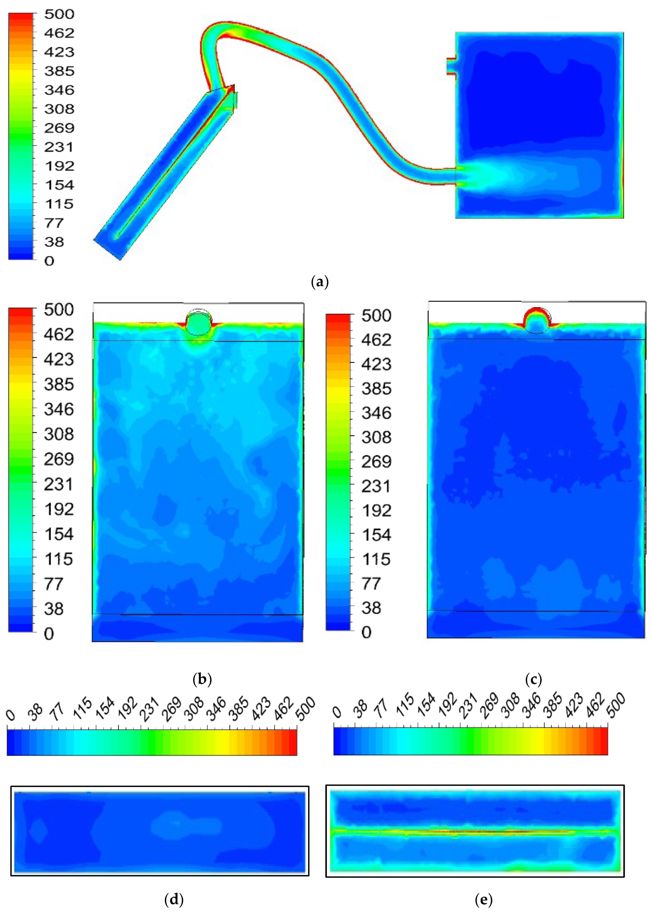
4.1. Velocity Fields

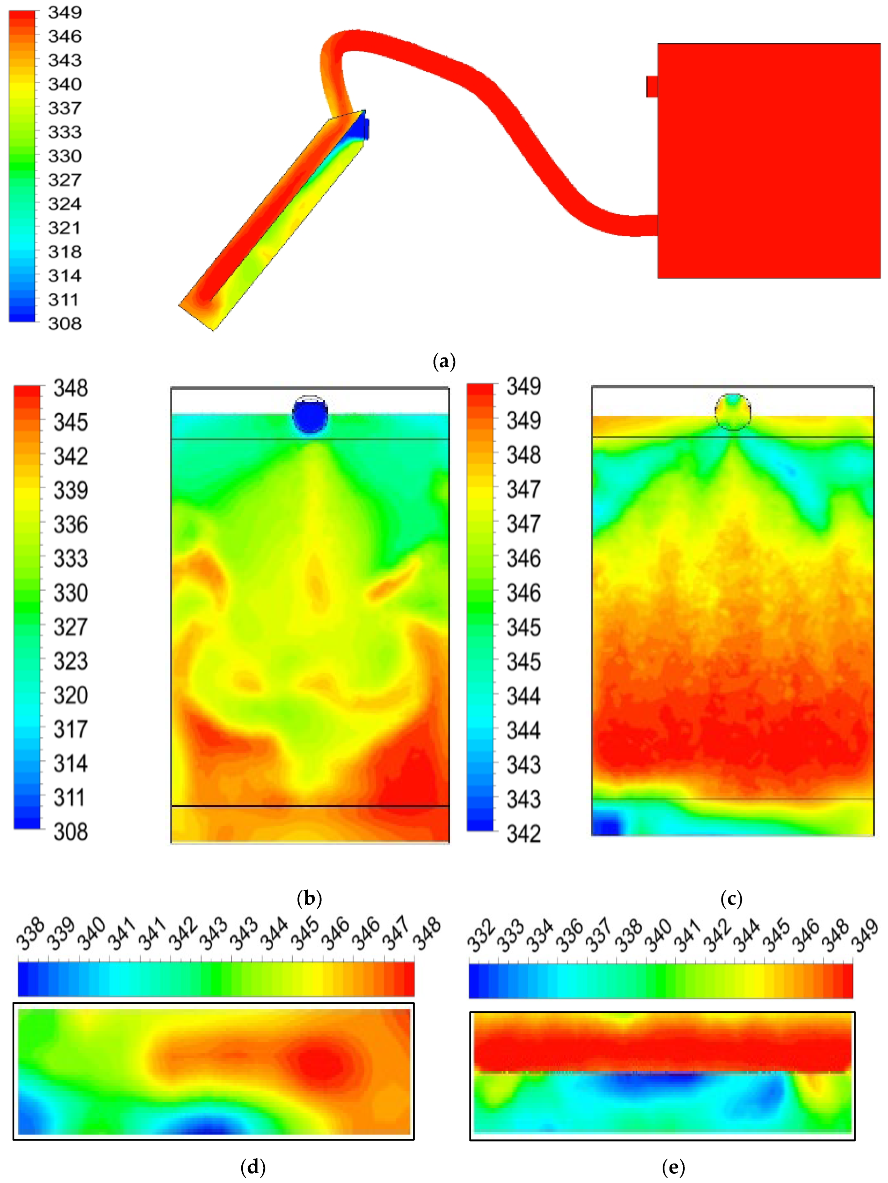
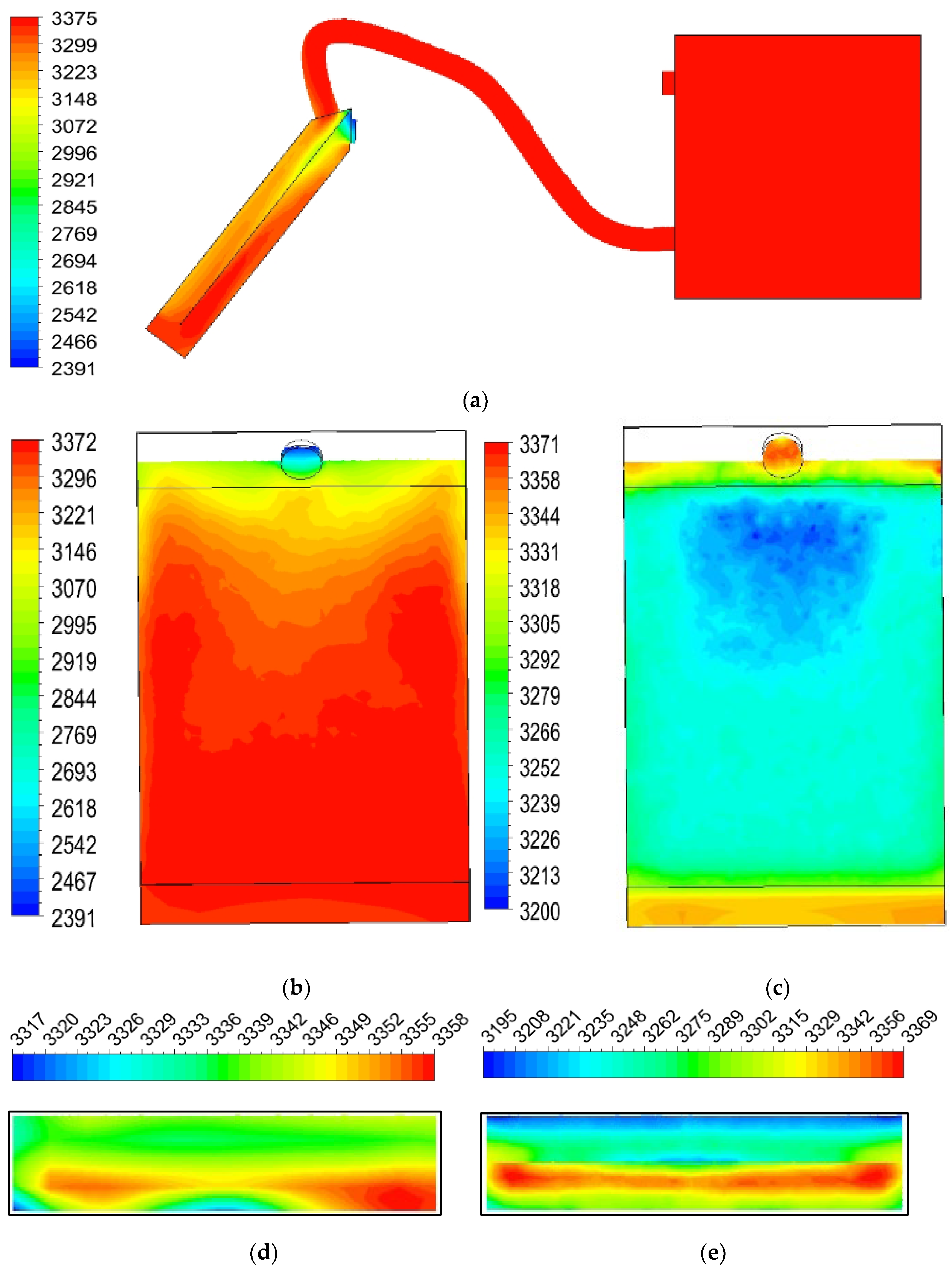
Figure 6 illustrates the velocity fields across various longitudinal and transverse planes within the first and second passages of the SAH system which reveals critical insights into the flow behavior and efficiency. In the longitudinal planes, the velocity profiles show the development of boundary layers and potential flow separation, with variations influenced by geometry and obstructions. The transverse planes highlight the distribution of velocity across the cross-section, indicating areas of high and low flow, and revealing any asymmetries or dead zones. These velocity patterns are essential for optimizing the design, improving flow uniformity, and enhancing heat transfer within the SAH system. Based on the obtained results, the first passage shows a flow decrease and the appearance of recirculation zones. Indeed, as the flow transitions to the second section, this effect becomes increasingly pronounced until the point of exit from the SAH. At this point, the speed of movement attains a velocity of V = 5 m/s. Subsequently, a discharge zone forms at the inlet hole of the box prototype via the conduit that divides the SAH from the prototype, extending towards the near wall. This phenomenon is contingent on the placement of the box prototype, which receives the heat flow from the SAH device pipe. In this area, the velocity changes, and two axial flows are detected: an upward flow, which creates a recirculation zone within the box prototype area, and a downward flow emerging at the bottom due to the presence of a dead zone. This movement persists through the outlet until the airflow exits, reaching a peak speed of V = 4 m/s. Within the discharge area, the average velocity stands at approximately V = 1.5 m/s, indicating significantly lower velocities in other areas.

4.2. Temperature

In the context of the first and second flows through the SAH device feeding the prototype, Figure 7 illustrates the temperature across different longitudinal and lateral sections. From these findings, it is observed that the temperature at the entrance is governed by the boundary condition which is set at 308 K. During the first flow, this temperature rises significantly, achieving an average of 338 K. In the subsequent flow, it escalates further to 349 K.

The temperature distribution across different longitudinal and lateral sections of the SAH system provides a comprehensive view of its thermal performance. Longitudinal sections reveal how temperature gradients develop along the flow path, indicating areas of heat gain or loss and highlighting thermal boundary layer development. These insights are crucial for optimizing thermal efficiency and ensuring a uniform temperature distribution throughout the system.

4.3. Radiation of the Heat Flux

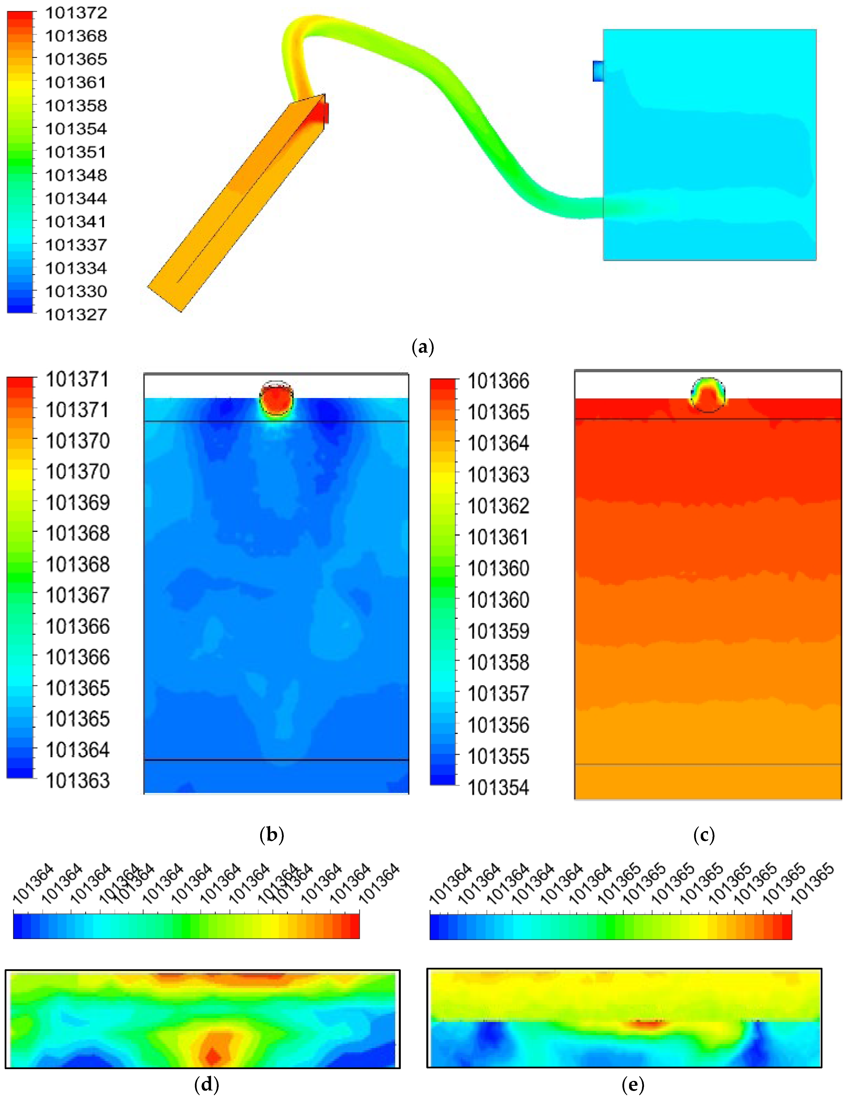
Figure 8 displays the distribution of the radiant heat flux across various longitudinal and lateral planes for the first and second flows through the SAH. From this analysis, it is noted that the radiation level at the SAH’s entry point starts at a minimal intensity of I = 2500 W·m⁻² in the central area of the initial flow. This intensity increases, peaking at I = 3375 W·m⁻² close to the absorber surface. However, during the second flow, there is a noticeable reduction in radiation levels, averaging at I = 3200 W·m⁻².

In the middle section of the second flow through the SAH device, the lowest observed radiation level is equal to I = 2650 W·m⁻². At this point, the radiation peaks at I = 3375 W·m⁻² across all areas of the box prototype, starting from the pipe inlet linked to the SAH. This peak value is maintained through to the outlet hole of the prototype.

The distribution of radiant heat flux across longitudinal and lateral planes for the first and second flows through the SAH system reveals critical insights into energy transfer efficiency. In the longitudinal planes, these patterns show how effectively solar energy is absorbed along the flow path, highlighting zones of peak absorption and potential energy losses. Analyzing these distributions helps to assess the overall performance and optimize the design to improve the uniformity and effectiveness of solar energy utilization within the SAH system.

4.4. Pressure

Figure 9 illustrates how pressure is distributed across both longitudinal and transverse sections during the initial and subsequent traverses through the SAH system feeding the prototype box. It reveals a zone of maximum compression at the collector’s entrance, where the highestpressure value is noted. Following this, the pressure diminishes and settles at a constant P = 101,365 Pa throughout the extent of both SAH system traverses. Towards the close of the second traverse, there is a continuous decline in pressure within the conduit, culminating in P = 101,347 Pa at the entrance to the prototype box.

The pressure distribution across the longitudinal and transverse sections during the initial and subsequent passages through the SAH system feeding the prototype box unveils the crucial airflow dynamics. This detailed pressure mapping is vital for optimizing the system design, ensuring an efficient airflow, and maintaining a consistent performance throughout the SAH system.

4.5. Turbulent Kinetic Energy

Turbulent kinetic energy denotes and represents the average kinetic energy per unit mass arising from eddies in turbulent flow, and is identified and calculated from the root-mean-square velocity fluctuations. This metric serves to quantify the turbulence intensity in fluid systems, essential for assessing its distribution and influence across applications like aerodynamics, industrial mixing, and environmental fluid dynamics. By assessing the turbulent kinetic energy, engineers and researchers can grasp the energetic dynamics of turbulent flows, informing better system designs and optimizing for enhanced operational effectiveness and efficiency.

Figure 9 illustrates how this turbulent kinetic energy is distributed across various longitudinal and transverse sections during the initial and subsequent flows through the SAH system into the box prototype. The findings indicate a distinct wake zone with the highest turbulent kinetic energy levels found near the SAH system’s collector inlet. This wake zone extends in the first flow close to the absorber side and reaches up to the mid-plane, as shown in Figure 10a,b.

Under these circumstances, the peak of the turbulent kinetic energy reaches a value of k = 0.95 m²·s⁻². Beyond this zone, the turbulent kinetic energy remains significantly low, except near the lower leading edge of the absorber where it reaches k = 0.08 m²·s⁻². Following the exit of the second passage, another wake zone indicative of the turbulent kinetic energy emerges and continues along the initial section of the conduit linking the SAH to the box. Subsequent to a reduction in the turbulent kinetic energy in the latter half of the conduit, a zone of expulsion becomes evident at the inlet hole of the box, extending to the discharge area up to the opposite wall. This phenomenon is attributed to a recirculation zone forming throughout the box prototype’s area. A marginal drop in the turbulent kinetic energy is noted outside of this zone. Nevertheless, at the box outlet, a wake zone signifying the turbulent kinetic energy is detected.

4.6. Specific Dissipation Rate

The specific dissipation rate measures how quickly kinetic energy converts into thermal energy within a fluid flow, offering a gauge of energy conversion efficiency. It indicates the frequency of this transformation, reflecting turbulence intensity and heat generation. This parameter is pivotal for understanding fluid dynamics, especially in turbulent environments like industrial processes or atmospheric studies. Engineers and researchers use specific dissipation rate analysis to enhance energy efficiency and optimize thermal management systems.

Figure 11 illustrates how this rate of dissipation varies across various longitudinal and transverse sections within the first and second passages of the SAH system that feeds into the box prototype. The findings reveal the formation of a wake zone exhibiting the highest specific turbulent dissipation rate beginning at the SAH system’s collector inlet, where the rate stands at a moderate ω = 300 s⁻¹. This zone extends through the first passage adjacent to the absorber side up to the central plane, as depicted in Figure 10a,b, where the specific dissipation rate peaks at ω = 500 s⁻¹. Beyond this region, the rate diminishes, dropping to a lower rate of ω = 40 s⁻¹ near the collector’s base, close to the insulator’s location. As the flow moves through the second passage, distancing itself from both the absorber and the glass, the specific dissipation rate falls further, eventually reaching zero in the upper half plane. However, within the conduit linking the SAH to the box, there is an upsurge in the dissipation rate, hitting a maximum again at ω = 500 s⁻¹.

When examining the two segments of the pipe, it is noteworthy that a steady decline in the dissipation rate was observed from the first to the second part. At the entrance of the hole leading into the box prototype, an expulsion zone emerges, extending through to the discharge area and up to the back wall. This phenomenon can be attributed to the formation of a recirculation zone throughout the entirety of the box prototype’s area. Additionally, a minor reduction in the specific dissipation rate is detected in the regions surrounding this zone. Nonetheless, at the box prototype exit, there has been a noticeable surge in the dissipation rate close to the wall.

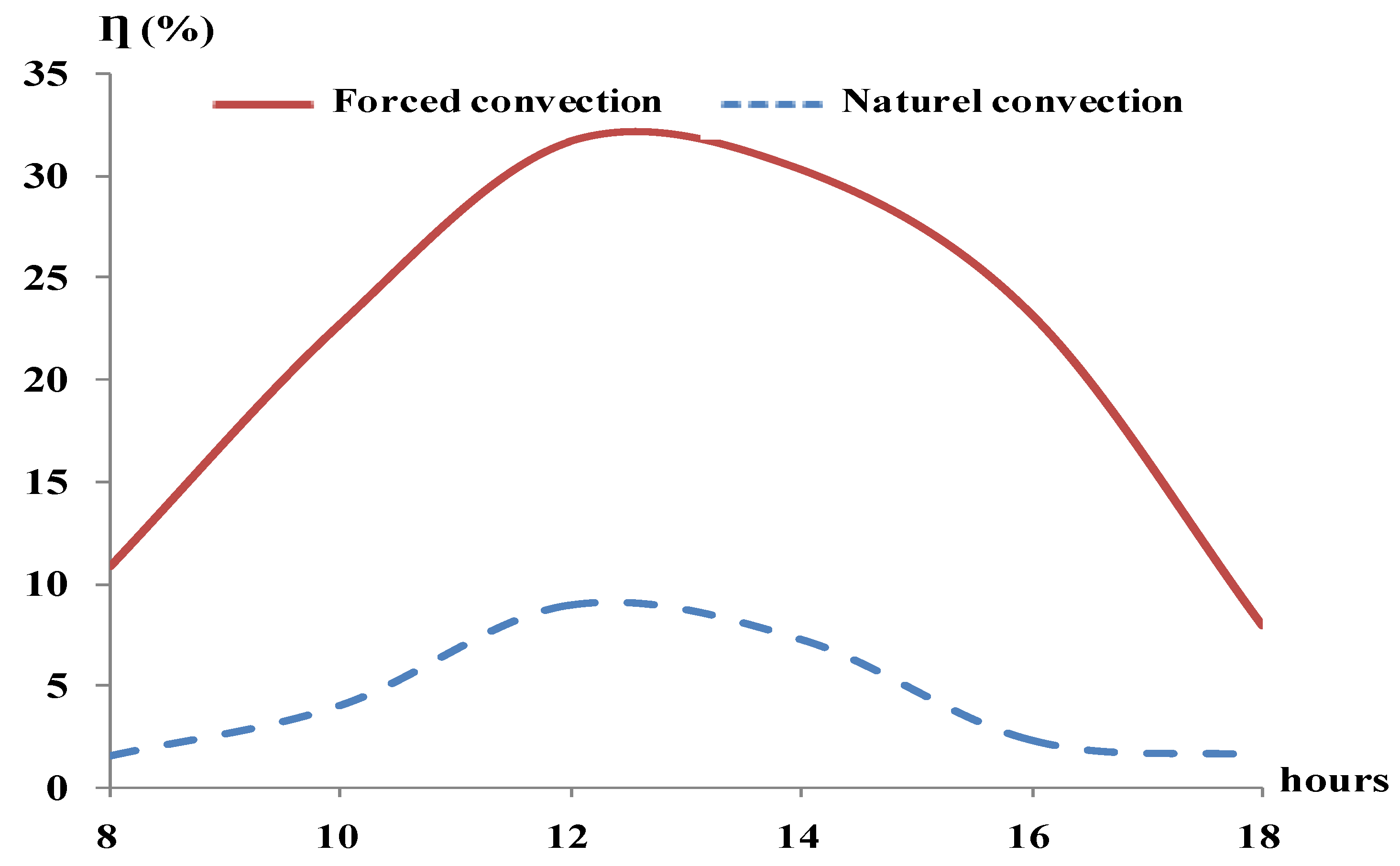
5. Energy Efficiency

Figure 12 presents a comparison of the energy efficiency profiles over time between the free and forced convection modes, derived using the following formula:

$$\mathsf{\eta }=\frac{\dot{\mathrm{m}}\hspace{0.17em}{\mathrm{c}}_{\mathrm{p}}\hspace{0.17em}({\mathrm{T}}_{\mathrm{out}}-{\mathrm{T}}_{\mathrm{in}})}{\mathrm{I}\mathrm{A}}$$

(15)

where

$\dot{\mathrm{m}}$: mass flow rate (kg·s⁻¹), c_p: specific heat capacity of the air at constant pressure (J·kg⁻¹·K⁻¹), T_out: outlet temperature (K), T_in: inlet temperature (K), I: solar radiation (W·m⁻²), A: area of the solar air heater (m²).

The shape and tendency of natural and forced convection efficiencies differ primarily due to their distinct mechanisms of heat transfer. Natural convection relies on buoyancy-driven flow caused by temperature differences, leading to a gradual increase in efficiency as thermal gradients strengthen and fluid circulation improves. The efficiency typically plateaus as the system reaches a steady state. In contrast, forced convection uses external mechanisms like pumps or fans to enhance the flow velocity over a surface, resulting in higher initial efficiencies that can further increase with higher flow rates. The relationship between efficiency and flow characteristics in forced convection tends to be more linear or positively accelerating, reflecting the direct control over heat transfer rates imposed by external forces. Thus, while natural convection follows a sigmoid or S-curve shape, forced convection exhibits a more responsive and potentially higher efficiency trend with an increased flow velocity. The findings indicate that energy efficiency starts off at relatively low levels at the day’s onset. As temperatures rise over the course of the day, energy efficiency correspondingly increases, peaking around noon with efficiency rates of η = 8.93% for free convection and η = 31.8% for forced convection. A significant improvement in the energy efficiency is observed, particularly in the morning, after t = 10 h. Into the afternoon, there is a steady decline in energy efficiency.

Under these circumstances, the relationship between the energy efficiency and time for the forced convection mode is given by the following equation:

η = 0.006 t⁴ − 0.339 t³ + 5.848 t² − 34.69 t + 62.34

(16)

For the natural convection, the correlated equation is written as follows:

η = 0.021 t⁴ − 1.1 t³ + 20.31 t² − 158.4 t + 446.5

(17)

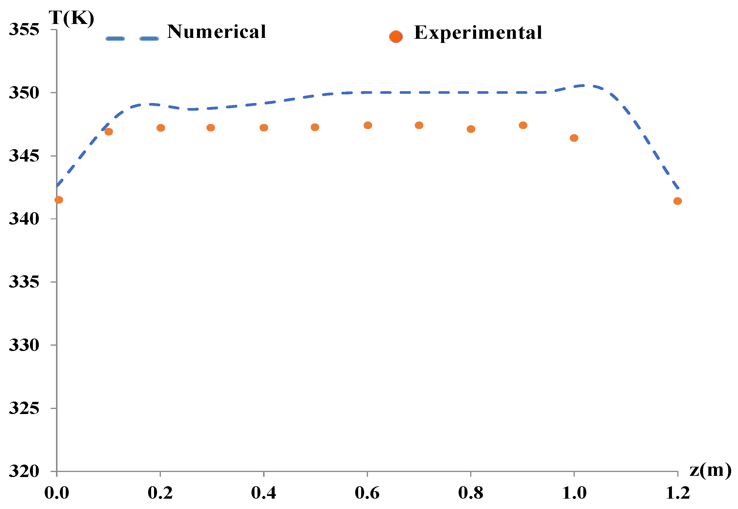
6. Comparison with Experimental Outcomes

Figure 13 displays the computational findings for temperature profiles within the second channel, juxtaposed with experimental outcomes when a fan is positioned alongside the insulation, operating in a delivery mode. The considered direction constitutes the principal tracked line of the heated airflow excluded from the outlet holes of the SAH system. Based on these findings, it is evident that the temperature attains a level of 343.10 K at the entry point of the second passage in the SAH system.

This value increases rapidly until 348.55 K and remains constant through the path of the airflow alongside the glass. Approaching the outlet holes of the SAH system, the temperature decreases until it reaches 340.30 K. On the other hand, the curves of the experimental and computational findings have a similar appearance across the board, with a 6% difference between them. As a result, the numerical method’s validity is confirmed by this good agreement.

7. Conclusions

This paper discusses the development and construction of a novel SAH test bench aimed at assessing the efficiency of solar systems. Specifically, the system in focus includes a dual-passage SAH configuration, divided by an absorber, and features a distribution fan positioned at the insulation’s inlet side. This fan is linked to a box via a conduit on the side of the glass. A piece of glass is then mounted on the device’s front side, with an absorber placed within. Consequently, this setup channels the flow of hot air into the box prototype, which is equipped with two circular openings on the same side; the entry opening acts as the hot air intake.

On the other hand, the outlet holes allow hot air to dissipate into the atmosphere. Numerical simulations were developed to investigate the turbulent flow in question. Under these conditions, the flow velocity deceleration and recirculation zones are visible in the first passage. This effect is more observable when the flow is transferred into the second passage. However, until its exit from the SAH system, the flow becomes uniform. Then, through the conduit separating the SAH from the prototype box, the discharge surface appears in the inlet holes and invades the opposite wall. On this side, velocity changes its direction and two axial flows are observed. Moreover, the flow causes the appearance of the recirculation region in the entire surface of the prototype. In fact, it is the dead zone, which has emerged in the down area, caused by the descending flow. This fact is due to the airflow entering at room temperature and passing into the passage between the absorber plate and the insulation, which begins to warm up. Then, the temperature of the airflow is more critical in the second passage because the movement between the glass and the absorber is influenced by the solar radiations. Thus, a continuous air heater heats the enclosure in this way.

This technology holds significant potential due to its ability to offer renewable energy and replace expensive traditional technologies, making it highly advantageous. Therefore, this research is valuable for comprehending airflow dynamics within indoor settings, underscoring the technology’s substantial benefits. Future research will explore how the geometry of the cabin prototype influences airflow characteristics.

References

1. Elsanossi, H.I. Performance analysis of solar air heater with different absorber material in single pass. Int. Res. J. Eng. Technol. 2018, 5, 2795–2801. [Google Scholar]
2. Abdullah, A.S.; Amro, M.; Younes, M.; Omara, Z.; Kabeel, A.; Essa, F. Experimental investigation of single pass solar air heater with reflectors and turbulators. Alex. Eng. J. 2020, 59, 579–587. [Google Scholar] [CrossRef]
3. Salmi, M.; Afif, B.; Akgul, A.; Jarrar, R.; Shanak, H.; Menni, Y.; Ahmad, H.; Asad, J. Turbulent flows around rectangular and triangular turbulators in baffled channels a computational analysis. Therm. Sci. 2022, 26, S191–S199. [Google Scholar] [CrossRef]
4. Singh, T.S.; Verma, T.N.; Jahiya, M.; Singh, P.K.; Kheiruddin, M.; Ajitkumar, K.; Singh, N.W.; Singh, H.D. Forced Convective Solar Air Heater: Effect of Thermal Storage Materials. Int. J. Appl. Eng. Res. 2018, 13, 5877–5880. [Google Scholar]
5. Zhou, C.; Wang, Z.; Chen, Q.; Jiang, Y.; Pei, J. Design optimization and field demonstration of natural ventilation for high-rise residential buildings. Energy Build. 2014, 82, 457–465. [Google Scholar] [CrossRef]
6. Abdulmunem, A.R.; Abed, A.; Hussien, H.; Samin, P.; Rahman, H. Improving the performance of solar air heater using high thermal storage materials. Ann. Chim.—Sci. Matér. 2019, 43, 389–394. [Google Scholar] [CrossRef]
7. Ostadijafari, M.; Dubey, A. Tube-Based Model Predictive Controller for Building’s Heating Ventilation and Air Conditioning (HVAC) System. IEEE Syst. J. 2021, 15, 4735–4744. [Google Scholar] [CrossRef]
8. Sharma, S.; Das, R.K.; Kulkarni, K. Computational and experimental assessment of solar air heater roughened with six different baffles. Case Stud. Therm. Eng. 2021, 27, 101350. [Google Scholar] [CrossRef]
9. Moradi, H.; Mirjalily, S.A.A.; Oloomi, S.A.A.; Karimi, H. Performance evaluation of a solar air heating system integrated with a phase change materials energy storage tank for efficient thermal energy storage and management. Renew. Energy 2022, 191, 974–986. [Google Scholar] [CrossRef]
10. Balakrishnan, V.; Gurunathan, M.; Parthasarathy, R.; Poluru, V.R. Experimental analysis of solar air heater using polygonal ribs in absorber plate integrated with phase change material. Therm. Sci. 2022, 26, 3187–3199. [Google Scholar] [CrossRef]
11. Chan, A.L.S. Investigation on the appropriate floor level of residential building for installing balcony, from a view point of energy and environmental performance: A case study in subtropical Hong Kong. Energy 2015, 85, 620–634. [Google Scholar] [CrossRef]
12. Homod, R.Z. Assessment regarding energy saving and decoupling for different AHU (air handling unit) and control strategies in the hot-humid climatic region of Iraq. Energy 2014, 74, 762–774. [Google Scholar] [CrossRef]
13. Rauf, A.; Crawford, R.H. Building service life and its effect on the life cycle embodied energy of buildings. Energy 2015, 79, 140–148. [Google Scholar] [CrossRef]
14. Boixo, S.; Diaz-Vicente, M.; Colmenar, A.; Castro, M.A. Potential energy savings from cool roofs in Spain and Andalusia. Energy 2012, 38, 425–438. [Google Scholar] [CrossRef]
15. Oliveira Panão, M.J.N.; Camelo, S.M.; Gonçalves, H.J. Assessment of the Portuguese building thermal code: Newly revised requirements for cooling energy needs used to prevent the overheating of buildings in the summer. Energy 2011, 36, 3262–3271. [Google Scholar] [CrossRef]
16. Nagaraj, M.; Reddy, M.K.; Sheshadri, A.K.H.; Karanth, K.V. Numerical Analysis of an Aerofoil Fin Integrated Double Pass Solar Air Heater for Thermal Performance Enhancement. Sustainability 2023, 15, 591. [Google Scholar] [CrossRef]
17. El-Sebaii, A.A.; Aboul-Enein, S.; Ramadan, M.; Shalaby, S.; Moharram, B. Thermal performance investigation of double pass-finned plate solar air heater. Appl. Energy 2011, 88, 1727–1739. [Google Scholar] [CrossRef]
18. Wazed, M.A.; Nukman, Y.; Islam, M. Design fabrication of a cost effective solar air heater for Bangladesh. Appl. Energy 2010, 87, 3030–3036. [Google Scholar] [CrossRef]
19. Sopian, K.; Alghoul, M.; Alfegi, E.M.; Sulaiman, M.; Musa, E. Evaluation of thermal efficiency of double-pass solar collector with porous-nonporous media. Renew. Energy 2009, 34, 640–645. [Google Scholar] [CrossRef]
20. Esen, H. Experimental energy and exergy analysis of a double-flow solar air heater having different obstacles on absorber plates. Build. Environ. 2008, 43, 1046–1054. [Google Scholar] [CrossRef]
21. Ozgen, F.; Esen, M.; Esen, H. Experimental investigation of thermal performance of a double-flow solar air heater having aluminum cans. Renew. Energy 2009, 34, 2391–2398. [Google Scholar] [CrossRef]
22. Teodosius, C.; Kuznik, F.; Teodosiu, R. CFD modeling of buoyancy driven cavities with internal heat source: Application to heated rooms. Energy Build. 2014, 68, 403–411. [Google Scholar] [CrossRef]
23. Han, H.J.; Jeon, Y.I.; Lim, S.H.; Kim, W.W.; Chen, K. New developments in illumination, heating and cooling technologies for energy-efficient buildings. Energy 2010, 35, 2647–2653. [Google Scholar] [CrossRef]
24. Satcunanathan, S.; Deonarine, S. A two-pass solar air heater. Sol. Energy 1973, 15, 41–49. [Google Scholar] [CrossRef]
25. Hassan, H.; Abo-Elfadl, S. Experimental study on the performance of double pass and two inlet ports solar air heater (SAH) at different configurations of the absorber plate. Renew. Energy 2018, 116, 728–740. [Google Scholar] [CrossRef]
26. Alam, T.; Kim, M.-H. Performance improvement of double-pass solar air heater—A state of art of review. Renew. Sustain. Energy Rev. 2017, 79, 779–793. [Google Scholar] [CrossRef]
27. Goodarzi, M.; Nouri, E. A new double-pass parallel-plate heat exchanger with better wall temperature uniformity under uniform heat flux. Int. J. Therm. Sci. 2016, 102, 137–144. [Google Scholar] [CrossRef]
28. Singh, S.; Dhiman, P. Thermal performance of double pass packed bed solar air heaters—A comprehensive review. Renew. Sustain. Energy Rev. 2016, 53, 1010–1031. [Google Scholar] [CrossRef]
29. Benguesmia, H.; Bakri, B.; Driss, Z.; Ketata, A.; Driss, S. Effect of the turbulence model on the heat ventilation analysis in a box prototype. Diagnostyka 2020, 21, 55–66. [Google Scholar]
Figure 1. (a)SAH test bench. (b) Geometrical arrangements.
Sustainability 16 06055 g001
Figure 2. Boundary conditions.
Sustainability 16 06055 g002
Figure 3. Meshing.
Sustainability 16 06055 g003
Figure 4. Velocity profiles.
Sustainability 16 06055 g004
Figure 5. Graphical planes.
Sustainability 16 06055 g005
Figure 6. Velocity field distribution: (a) along the longitudinal plane; (b) within the first passage; (c) through the second passage; (d) across the first transverse plane; and (e) over the second transverse plane.
Sustainability 16 06055 g006
Figure 7. Distribution of the temperature. (a) along the longitudinal plane; (b) within the first passage; (c) through the second passage; (d) across the first transverse plane; and (e) over the second transverse plane.
Sustainability 16 06055 g007
Figure 8. Distribution of the radiation of the heat flux. (a) along the longitudinal plane; (b) within the first passage; (c) through the second passage; (d) across the first transverse plane; and (e) over the second transverse plane.
Sustainability 16 06055 g008
Figure 9. Distribution of the pressure. (a) along the longitudinal plane; (b) within the first passage; (c) through the second passage; (d) across the first transverse plane; and (e) over the second transverse plane.
Sustainability 16 06055 g009
Figure 10. Distribution of the turbulent kinetic energy. (a) along the longitudinal plane; (b) within the first passage; (c) through the second passage; (d) across the first transverse plane; and (e) over the second transverse plane.
Sustainability 16 06055 g010
Figure 11. Distribution of the specific dissipation rate. (a) along the longitudinal plane; (b) within the first passage; (c) through the second passage; (d) across the first transverse plane; and (e) over the second transverse plane.
Sustainability 16 06055 g011
Figure 12. Energy efficiency profiles.
Sustainability 16 06055 g012
Figure 13. Temperature profiles in the second channel.
Sustainability 16 06055 g013