Article

Trend and Variability Analysis of Annual Maximum Rainfall Using Observed and Remotely Sensed Data in the Tropical Climate Zones of Uganda

Department of Civil Engineering, Stellenbosch University, Private Bag X1, Matieland 7602, South Africa
*
Author to whom correspondence should be addressed.
Sustainability 2024, 16(14), 6081; https://doi.org/10.3390/su16146081
Submission received: 3 May 2024 / Revised: 9 July 2024 / Accepted: 13 July 2024 / Published: 16 July 2024

Abstract

:
Understanding rainfall variability and trends is crucial for effective water resource management and disaster preparedness, particularly in tropical regions like Uganda. This study analyzes the trends and variability of the Annual Maximum Series (AMS) and seasonal rainfall data across four rainfall stations in Uganda, comparing observed data with various Remotely Sensed Rainfall (RSR) products. The key methods used in this study include the Mann–Kendall test and Sen’s slope estimator for trend analysis, AMS rainfall variability analysis using statistical performance metrics such as the Nash–Sutcliffe Coefficient of Efficiency (NSE) and Percent Bias (PBIAS), and data distribution comparisons based on goodness-of-fit evaluation using the Kolmogorov–Smirnov (KS) test. The results indicate that most trends in the seasonal rainfall and AMS data are statistically insignificant. However, the September to November (SON) observed rainfall at the Gulu station shows a statistically significant increasing trend of 7.68 mm/year (p-value = 0.03). Based on the PBIAS metric, GPCC and NOAA_CPC products outperform other RSR data products. At the Jinja station, NOAA_CPC has a PBIAS value of −12.93% and GPCC, −14.64%; at Soroti, GPCC has −9.66% and NOAA_CPC, −14.79%; at Mbarara, GPCC has −5.93% and NOAA_CPC, −11.63%; and at Gulu, GPCC has −3.05% and NOAA_CPC, −19.23%. The KS test results show significant differences in the distribution of RSR data and observed rainfall data, though GPCC shows significant agreement at the Gulu (p-value = 0.60) and Mbarara (p-value = 0.14) stations. Additionally, NOAA_CPC outperforms other RSR data products at the Mbarara station, with a KS p-value of 0.24. This study highlights the limitations of current RSR datasets in replicating observed AMS rainfall data. Based on KS test results, GPCC is identified as a better product for hydrological applications at the Gulu, Jinja, and Soroti station areas compared to other RSR products. For the Mbarara station, NOAA_CPC outperforms other RSR products.

1. Introduction

Uganda has a diverse climate landscape, subdivided into nine distinctive climatic zones (Figure 1). Among these zones, tropical climates are predominant, encompassing the tropical rainforest (Af), tropical monsoon (Am), and tropical savannah (Aw) categories. These tropical zones collectively account for 96.5% (estimated from the Köppen–Geiger climate classification map using ArcGIS 10.8. 2 software) of the total land surface area.
Trewin [1] noted that tropical regions are characterized by relatively stable temperatures, but exhibit strong seasonal variations in rainfall. The 2020 World Bank report noted that the frequency and intensity of extreme weather events, including floods, droughts, and landslides, have risen markedly over the past 30 years in Uganda [2]. This increase is largely attributed to more intense rainfall patterns, which not only lead to more frequent flooding but also magnify the impact due to the expansion of infrastructure, human settlements, and overall national development. Specific areas like Gulu District face significant challenges during the rainy seasons, with roads becoming impassable, cutting off access to critical services such as health facilities and schools. Furthermore, the same World Bank report notes that floods in Uganda annually affect nearly 50,000 people and result in losses exceeding $62 million. The recent floods of April 2024 caused widespread displacement, loss of life, crop destruction, and hindered access to essential services such as healthcare, education, and business operations according to the 2024 International Federation of Red Cross (IFRC) report for Uganda [3]. The floods affected approximately 14 districts and displaced 4463 families since April 2024. The issue of floods is recurrent across several districts in Uganda, particularly in the Western, Central, and Eastern regions. In his publication, Onyutha [4] noted several flood–prone areas in Uganda, including Western regions like Kasese and Eastern regions such as Mbale, Soroti, and Kumi, along with the Central regions. He pointed to several historical floods experienced in the country in the years 2007, 2010, 2013, up to 2016. Furthermore, he noted that understanding extreme rainfall events is directly linked to strategic planning and the management of risk in hydrometeorological applications.
Despite ongoing efforts by government agencies, including the Uganda National Roads Authority (UNRA), municipal councils, and district local governments, to repair and rehabilitate roads, bridges, and culverts, these infrastructures are often destroyed repeatedly. This cycle of damage and repair underscores the importance of understanding rainfall trends and variability. By incorporating the effects of increasing trends and variabilities, we can design more resilient hydrological structures capable of withstanding the intensified rainfall threats in the tropical regions of Uganda. Hydrological structures such as culverts, stormwater drainage channels, bridges, and spillways play a pivotal role in managing storm water resources, and their design necessitates the consideration of various parameters, with peak discharge derived from rainfall intensity being a critical one. Rainfall intensity can be estimated using several methods, with intensity–duration–frequency (IDF) curves being a widely used approach. IDF curves are a global tool, extensively employed in the design, operation, and maintenance of various hydrological and water management infrastructure, as noted by Andre et al. [5]. According to Wageningen and Du Plessis [6], engineers rely on a design discharge, corresponding to a specific storm duration and return period obtained from IDF curves, to appropriately size these structures. IDF curves are constructed using AMS rainfall data for different storm durations curves, as noted by Jokowinarno et al. [7]. Thus, the frequency of heavy rainfall (highest 24 h rainfall) is of significant interest to hydrologists for several reasons, including the design of hydrological and hydraulic structures such as bridges, culverts, and flood alleviation schemes according to Robinson and Ward [8]. By analyzing the AMS, hydrologists can estimate the probability and return period of extreme rainfall events, which is crucial for designing flood defenses and managing flood risks. Engineers use AMS data to ensure that hydrological structures can withstand extreme rainfall events of specific magnitudes and return periods. Additionally, the AMS is used to detect trends and changes in the frequency and intensity of extreme rainfall events over time, aiding in understanding the impacts of climate change on weather extremes. Additionally, in areas where ground-based observed rainfall data are non–existent, suitable RSR products offer an alternative worth investigating. Within Uganda, the Word Bank report [2] and Luwa et al. [9] noted that there is a persistent limitation regarding the availability of observed rainfall data across the country. This highlights the necessity of exploring the usability of available open-source RSR data. Moreover, understanding the nature of seasonal rainfall trends can inform effective strategic water resource management and disaster risk preparedness.
Extreme rainfall events have been extensively studied worldwide, including in regions like Bangladesh, Peninsular Malaysia, Germany, and Africa, as noted by Onyutha [4]. In Uganda, research into extreme rainfall events has been undertaken by various authors and organizations such as the World Bank. The World Bank [2] reported an increase in the intensity of rainfall during the SON season, with a reduction in the March–April–May (MAM) rainfalls. Nsubuga et al. [10] studied seasonal rainfall trends across Uganda from 1940 to 2009 using statistical methods such as the Mann–Kendall test and Sen’s slope estimator. Another significant study by Majaliwa et al. [11] examined historical seasonal and annual rainfall trends across eight climatologically homogenous zones in Uganda for the period 1970–2000, employing regression analysis to conduct trend tests. In their 2016 study, Ogwang et al. [12] employed the Mann–Kendall analysis to investigate the sudden changes in the mean SON rainfall across the country using Climate Research Unit rainfall data for 1901 to 2013. In neighboring Kenya, Macharia et al. [13] assessed the accuracy of various RSR products in predicting rainfall patterns between 1998 and 2013, utilizing statistical performance metrics like Mean Error (ME), Mean Absolute Error (MAE), Root Mean Square Error (RMSE), and Coefficient of Determination (R2). Among the RSR products evaluated by Macharia et al. [13] were the gauge-interpolated Global Precipitation Climatology Centre (GPCC) product and the reanalysis Modern-Era Retrospective Analysis for Research and Applications (MERRA) product.
Despite the previous research conducted by various authors and organizations, there remains some knowledge and information gaps in hydrological-specific studies, particularly concerning the analysis of AMS rainfall data. Studies undertaken in Uganda by organizations such as the World Bank [2], and by authors like Luwa et al. [9], Nsubuga et al. [10], and Egeru et al. [14], focused on analyzing trends in seasonal and annual rainfall totals. However, these studies fall short of the daily temporal resolution required for estimating discharge for hydrological infrastructure design. Additionally, the viability of readily available RSR products as alternatives to observed data has not been sufficiently evaluated. This evaluation is particularly necessary in areas where ground-based rainfall data are scarce or non–existent, which is often the case in remote locations. Furthermore, while the World Bank [2] report noted an increase in extreme weather events over the past 30 years, existing research in Uganda—conducted by scholars such as Onyutha [4], Nsubuga et al. [10], Majaliwa et al. [11], and Ogwang et al. [12]—did not cover the critical period from 1991 to 2020. This period reflects the current global climate zoning, as indicated by Beck et al. [15], and is defined by the World Meteorological Organization (WMO) as the latest climate normal period [16]. Structuring climate periods in 30-year intervals facilitates easier comparison of results across the same timeframe.
The primary objective of this research is to conduct seasonal and AMS rainfall trend analysis, and to analyze the variability of AMS observed rainfall data compared to RSR data products. The specific objectives of this study are:
  • To analyze the trends of MAM and SON seasonal rainfall.
  • To analyze the trends of AMS observed rainfall and RSR datasets.
  • To assess the variability in the AMS between observed rainfall and RSR datasets.
  • To evaluate the fit between observed rainfall and RSR data distributions.
This study tests the following hypotheses:
  • Are there significant trends in MAM and SON seasonal rainfall?
  • Do AMS rainfall data show significant trends across the different climatic zones?
  • Are there identifiable patterns of variability in RSR AMS data comparable to observed AMS rainfall data?
  • Does the distribution of RSR datasets significantly differ from observed AMS rainfall data?
The significance of this research lies in its potential to enhance strategic planning and management of hydrological infrastructure. Understanding seasonal rainfall trends can inform better water resource management strategies and boost community resilience against climate-related risks. Furthermore, the results of comparative analysis of observed and RSR datasets offer viable alternatives to traditionally observed rainfall data in areas where ground-based rainfall monitoring is non-existent.

2. Materials and Methods

2.1. Description of the Study Area

Uganda, a landlocked country situated in the East Africa region (Figure 1), has a surface area totaling approximately 241,550 square kilometers. Within this surface area, 41,743 square kilometers (equivalent to 17.2%) is characterized by open water bodies and swamps, while the remaining 199,807 square kilometers constitute open land according to Majaliwa et al. [11] and the Ministry of Water and Environment (MWE) [17]. Uganda has a diverse climate landscape, subdivided into nine distinctive climatic zones, as illustrated in Figure 1. The climate zones were extracted from the Köppen–Geiger global climate classification raster data by Beck et al. [15] for the period 1991–2020, with a spatial resolution of 1 km by 1 km.
Uganda experiences two distinct rainfall seasons in the Eastern, Southern, and Western regions, whereas the Northern region experiences only one rainfall season. The two rainfall seasons occur from March to May (MAM) and from September to November (SON). The World Bank report [2] noted a reduction in the MAM season rainfall and the Uganda National Meteorological Authority (UNMA) report [18] noted an increase in the SON season rainfall. In the Northern region, a single extended rainfall season prevails, spanning from March to mid–October. As a general overview, the country typically receives an annual average of 1200 mm of rainfall according to MWE [17]. The monthly average rainfall exhibits variations, with January experiencing slightly less than 50 mm of rainfall and October receiving slightly more than 150 mm of rainfall on average according to the World Bank report [2].

2.2. Rainfall Datasets

The rainfall data used in this research cover a 30-year period from 1 January 1991 to 31 December 2020. As mentioned earlier, this period of 1991–2020 is the current global climatic zoning by Beck et al. [15] and is defined by the WMO [16] as the latest climate normal period. Furthermore, the data length of 30 years is considered sufficient for hydrological studies, as noted by Raes [19].

2.2.1. Observed Rainfall Data

The daily observed rainfall data of four stations, i.e., Jinja, Soroti, Gulu, and Mbarara, were obtained from the UNMA. These stations were chosen for their consistent and continuous data and were located at airstrips across the country, with Gulu in the north, Soroti in the east, Jinja in the Central region, and Mbarara in the southwest. The Gulu, Soroti, and Mbarara stations fall within the tropical savannah climate zone, while Jinja is in the tropical rainforest climate zone (Figure 1). The Gulu and Soroti stations are located north of the equator, while the Mbarara station is located south of it.

2.2.2. Remotely Sensed Rainfall Products

In this research, RSR products, commonly known in the literature as gridded precipitation products, are categorized as follows:
  • Gauge-only products: These rely exclusively on observations from rain gauge stations, using various interpolation methods to construct the data. An example includes the Global Precipitation Climatology Centre daily rainfall product, which solely utilizes rain gauge data. This product is often available at a coarser spatial resolution exceeding 0.5° according to Macharia et al. [13] and Duan et al. [20]. GPCC data can be accessed from: https://opendata.dwd.de/climate_environment/GPCC/full_data_daily_v2022/ (accessed on 16 June 2024).
  • Satellite-gauge combined products: These integrate gauge-only and satellite-only data through various bias correction or blending procedures:
    • Climate Hazards Group Infrared Precipitation with Stations (CHIRPS): This product merges rain gauge measurements with satellite observations. It offers a spatial resolution of 4.8 km and covers latitudes between 50° N and 50° S from 1981 to the near present according to Du Plessis and Kibii [21].
    • National Oceanic and Atmospheric Administration Climate Prediction Centre (NOAA_CPC): Developed from the CPC Unified Precipitation Project, this product combines a global dataset (55 km resolution) and a dataset for the conterminous United States (28 km resolution), providing daily data from 1979 to the near present.
    • The Precipitation Estimation from Remotely Sensed Information using Artificial Neural Networks (PERSIANN)—Climate Data Record (CDR) is a rainfall dataset offering a 24 km spatial resolution with daily updates, covering the period from 1983 to the near present. It spans latitudes from 60° N to 60° S. Developed by the Centre for Hydrometeorology and Remote Sensing (CHRS) at the University of California, Irvine, this dataset leverages remotely sensed data processed through artificial neural networks to estimate precipitation according to Macharia et al. [13] and Duan et al. [20]. Further information can be found at: https://chrsdata.eng.uci.edu/ (accessed on 16 December 2022).
  • Numerical weather prediction products: These rainfall products from atmospheric models use a combination of satellite and in situ observations:
    • MERRA2: Developed by NASA’s Global Modeling and Assimilation Office, MERRA2 offers data with a spatial resolution of 50 km, covering the period from 1980 to the near present according to [13].
    • European Centre for Medium-Range Weather Forecasts (ECMWF) reanalysis version 5 (ERA5): This fifth-generation global reanalysis dataset provides a daily precipitation dataset with a spatial resolution of 24 km from 1979 to the near present, available through the climate data store: https://cds.climate.copernicus.eu/cdsapp#!/home (accessed on 16 December 2022).
    • ERA5_AG (for Agriculture): Specifically designed for agricultural and agro-ecological applications, this dataset offers daily precipitation data at a spatial resolution of 9.6 km from 1979 to the near present. The data is developed by ECMWF’s Copernicus climate change service and is available at: https://cds.climate.copernicus.eu/cdsapp#!/home (accessed on 16 December 2022).
The selection of these RSR data products for evaluations was based on the length of data records (1991–2020), temporal resolution (daily), and open-source availability, ensuring that they are readily accessible. The RSR data of the same temporal resolution were extracted from the same point locations as the observed rainfall data for direct comparisons and point-based analysis.

2.2.3. Annual Maximum Series Rainfall Data

The Annual Maximum Series (AMS) refers to a time series composed of the maximum value of a specific variable, in this case, rainfall, recorded each year over a specified period at a particular location. For hydrological studies, the AMS typically represents the highest daily rainfall (24 h) amount observed each year according to Subramanya [22].
To construct the AMS rainfall data, daily rainfall records are collected over a specific period, ideally spanning multiple years. For each calendar year, the day with the highest recorded 24 h rainfall is identified. This maximum 24 h rainfall value represents the annual maximum for that year. These annual maximum values are then compiled into a time series, resulting in a dataset where each entry represents the maximum daily rainfall for a given year.

2.3. Methodology

Figure 2, the methodology flow chart, illustrates the sequential steps undertaken for the analysis of AMS rainfall trends in both observed and satellite-based datasets. The process commences with rainfall data pre-processing, encompassing data quality checks. Subsequently, the data undergo analysis, involving homogeneity and normality tests, followed by the extraction of daily AMS rainfall data values. Lastly, the data are evaluated by conducting trend analysis, employing the Mann–Kendall method, and quantifying the magnitudes of these trends through the application of the Sen slope’s method.

2.3.1. Data Pre-Processing

  • Rainfall data quality control
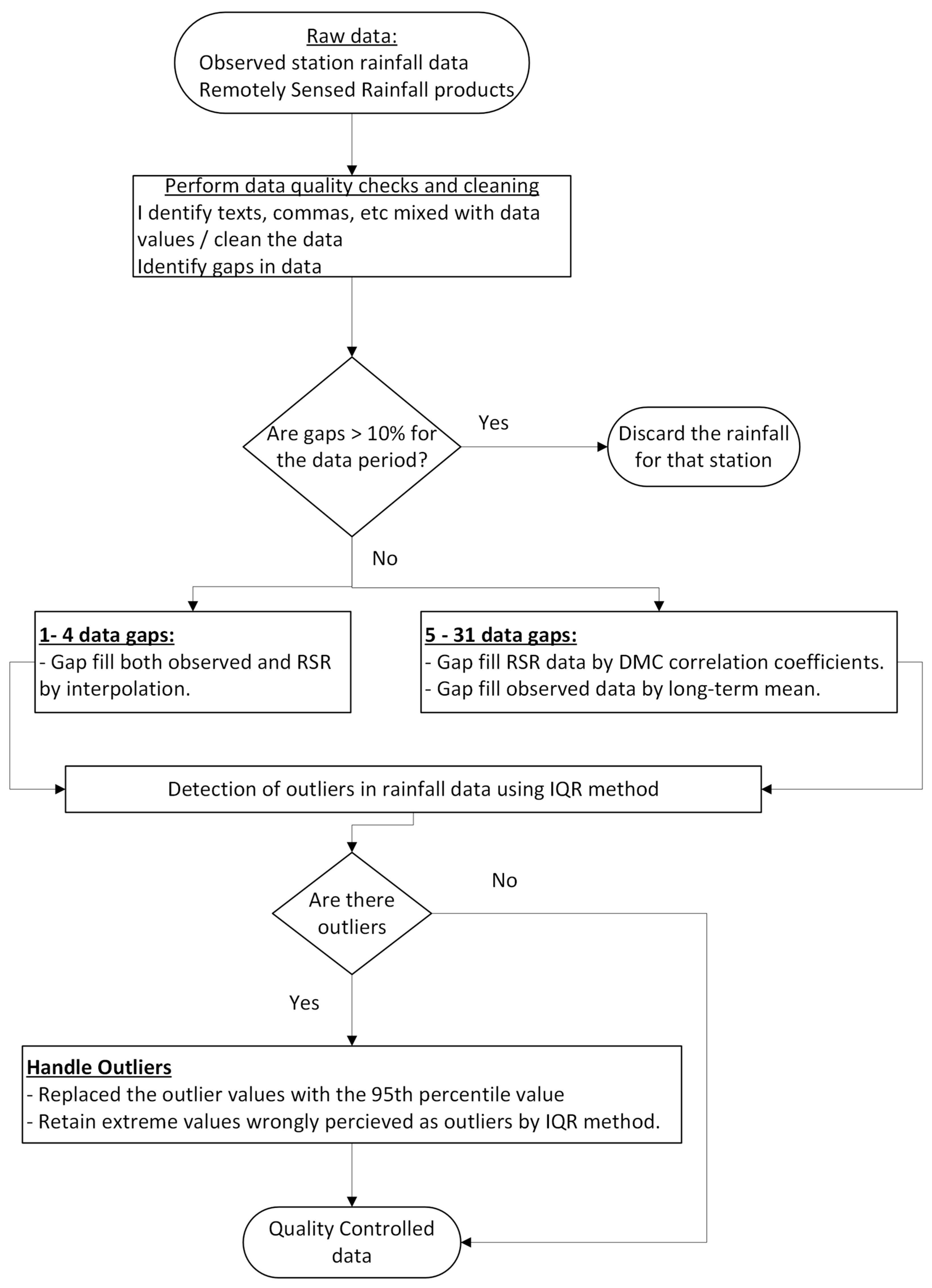
Both the observed and RSR daily rainfall data underwent rigorous data quality checks and control, as outlined in the flow chart depicted in Figure 3. Prior to analysis, the data were subjected to standard quality assessments that included verifying continuity over time (to identify gaps in the rainfall time series); checking for the presence of texts, commas, and symbols mixed with rainfall data; ensuring data coverage for the study period from 1991 to 2020; and identifying outliers (which may represent either erroneous entries or extreme values). The detailed procedures for these quality checks are described in Subramanya [22].
  • Gap filling of observed rainfall data
Following the procedure outlined in the methodological flow chart (Figure 3), gaps in the observed time series were filled using two methods: linear interpolation and long-term mean averages (arithmetic mean). Specifically, gaps spanning 1 to 4 days were addressed through linear interpolation, while longer gaps ranging from 1 to 31 days were filled using the long-term mean. In their study, Nsubuga et al. [10] similarly utilized the long-term mean to address data gaps of up to one month. This approach involved the following steps: Each missing value in the rainfall data was matched with the corresponding day of the month. It was then replaced with the long-term mean rainfall calculated specifically for that day. For example, if rainfall data for the 1st of January were missing, the gap would be filled using the historical average rainfall for the 1st of January.
  • Gap filling of RSR data products
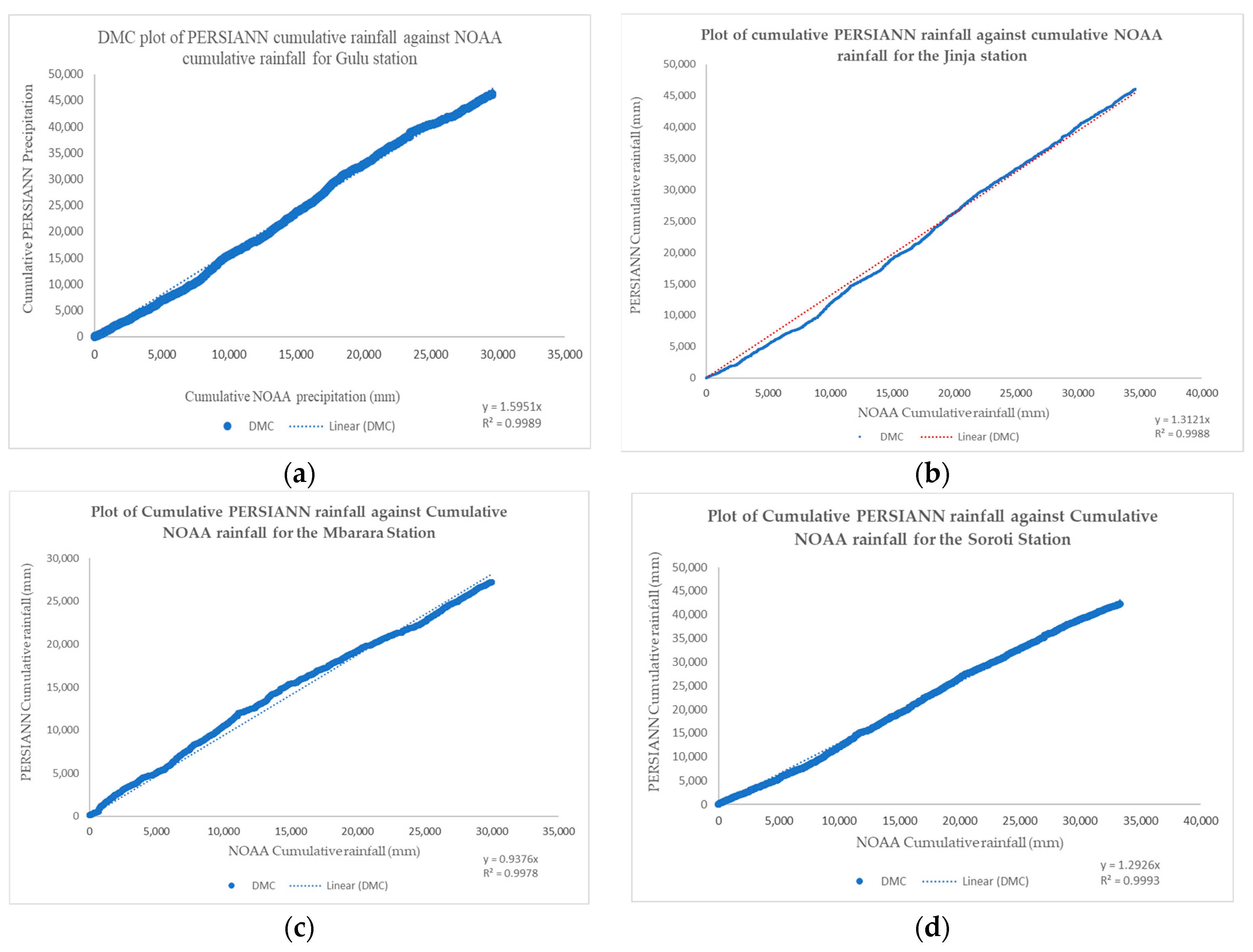
To address gaps in the RSR rainfall data, a two-step process was implemented. Firstly, linear interpolation was utilized for gaps lasting 1 to 4 days. Secondly, for longer gaps ranging from 1 to 31 days, station correlation coefficients derived from Double Mass Curve (DMC) plots were employed to estimate the missing values, as indicated in Equation (1). For the NOAA_CPC satellite rainfall product, which had data gaps of 1 to 2 days, linear interpolation was used for gap filling. The gaps in the PERSIANN data were filled by multiplying the NOAA data values (at the same location as PERSIANN) by the correlation coefficients from the DMC plots (Figure A1) shown in Appendix A. Table 1 lists the equations derived from the DMC plots, which were used to estimate the missing rainfall data values.
y = m x
where:
-
y represents the missing PERSIANN rainfall data value;
-
m denotes a constant derived from the Double Mass Curve (DMC) plot;
-
x represents the NOAA rainfall data value.
Table 1. Equations for estimating missing rainfall data values in PERSIANN satellite product.
Rainfall StationCorrelation CoefficientEquationR2 Value
Jinja1.312 y = 1.3121 x 0.9988
Soroti1.2926 y = 1.2926 x 0.9993
Gulu1.5951 y = 1.5951 x 0.9989
Mbarara0.9376 y = 0.9337 x 0.9978
  • Outlier detection
The Interquartile Range (IQR) method, a widely used non-parametric tool for detecting outliers in datasets, was utilized alongside visual inspection of time series rainfall data plots to identify stark anomalies in some values. The IQR method is based on the principles of the boxplot and calculates the IQR as the difference between the 75th percentile (Q3) and 25th percentile (Q1) of the data. Data points that fall below (Q1 − 1.5 × IQR) or above (Q3 + 1.5 × IQR) are typically considered outliers according to Zhao and Yang [23]. The outlier data values were corrected with the 95th-percentile values for the respective years.
  • Homogeneity test
Following the daily data quality test processes, homogeneity tests were applied to all the daily rainfall datasets to assess their consistency over time. The homogeneity tests applied included the Pettitt test, Standard Normal Homogeneity Test (SNHT), Buishand Range (BR) test, and von Neumann test. These methods are among the most widely recognized and commonly utilized homogeneity testing techniques according to Bickici and Kahya [24] and Mohammed and Scholz [25]. Of these methods, the Pettitt test was selected due to its non-parametric nature according to Kocsis et al. [26]. The Pettitt approach does not rely on any underlying assumptions, such as the normality of the rainfall data distribution. The null and alternative hypotheses for the homogeneity test were: H0: Data are homogeneous and Ha: There is a date at which there is a change in the data. A p-value greater than the significance level of alpha = 0.05 indicated that the null hypothesis could not be rejected, while a p-value lower than the significance level of alpha = 0.05 indicated that the null hypothesis should be rejected. The homogeneity tests on the daily rainfall data were performed using an XLSTAT Version 2023.1.2 application in a Microsoft Excel environment.

2.3.2. Data Analysis

  • Trend Analysis
The methodology employed for trend analysis was a combination of the Mann–Kendall (MK) test and the Sen slope (illustrated in flow chart, Figure 4). This approach was selected for three main reasons: First, the MK test is a widely used non-parametric method for detecting monotonic trends in various data types, including environmental, climate, and hydrological datasets according to Pohlert [27]. This method has also been utilized in Uganda by Nsubuga et al. [10] and Ogwang et al. [12] for trend analysis of rainfall data. Second, the method does not assume any specific underlying distribution for the data according to Nsubuga et al. [10] and Maity [28]. Third, it is robust against outliers in the dataset, as noted by Nsubuga at al. and other authors [10,27,28]. The test was used to detect monotonic trends in the data series, while the Sen slope was used to estimate the magnitude of these trends.
The trend analysis was conducted using the XLSTAT application within the MS Excel environment. The null and alternative hypotheses used for the trend analysis test were: H0: There is no trend in the series and Ha: There is a trend in the series. A p-value greater than the significance level of alpha = 0.05 indicated that the null hypothesis could not be rejected, while a p-value lower than the significance level of alpha = 0.05 indicated that the null hypothesis should be rejected. The step-by-step approach for performing the Mann–Kendall test is presented in a flow chart (Figure 4) and is outlined below. Further elaboration on the method is provided in Maity [28] and Meals and Spooner [29]:
  • Step 1: Prepare the rainfall data
  • Quality Control: The data underwent a quality control process as depicted in Figure 3.
  • Data Extraction and Organization: AMS rainfall data were extracted and organized to facilitate the computation of the MK statistics, S. Additionally, for seasonal trend analysis, the rainfall totals for MAM and SON were calculated and properly organized.
  • Step 2: Compute the MK statistic (S)
  • Compute the differences in data points. For each data point, xi, compute the difference with all subsequent data points, xj.
  • Calculate the sign function. For each pair (xi, xj), determine the sign of (xj − xi)
Sum the Signs (S). Add all the sign values together to obtain the MK test statistics.
The MK test statistic, S, is calculated using Equation (2) according to Pohlert and several other authors [27,30,31,32,33,34,35]:
S = i = 1 n 1 j = i + 1 n s g n x j x i
The test computes the difference between the time series values in the later year with all the early years (xj − xi), where j is the later year and i represents the early years; therefore, in all cases j > i. The xj and xi are time series and n is the number of data points in the time series. The “sgn” sign function is expressed as shown in Equation (3):
s g n x j x i = + 1 ,     w h e n   x j x i > 0   0 ,     w h e n   x j x i = 0 1 ,     w h e n   x j x i < 0
  • Step 3: Calculate the variance of S
The variance of the Mann–Kendall test, Var(S), is given by Equation (4) according to Rahman and Azim [36]:
V a r S = n n 1 2 n + 5 i = 1 m t i i i 1 2 i + 5 / 18
where ti is the number of ties up to sample i.
  • Step 4: Compute the test statistic (Z)
The standardized test statistic, Zc, is given by Equation (5):
Z c = S 1 V a r S ,     w h e n   S > 0 0 ,                                       w h e n   S = 0 S + 1 V a r S ,     w h e n   S < 0
  • Step 5: Results and interpretation
  • If the Zc value exceeds the critical value of 1.96, corresponding to a 95% confidence level (5% significance level), reject the null hypothesis that there is no trend.
  • The negative value of Zc indicates a decreasing trend, while the positive value indicates an increasing trend.
  • Sen’s slope estimator
The most widely used method to estimate the magnitude of rainfall trends is Sen’s Slope Estimator Test according to Rahman and Azim [36]. The method is not affected by data outliers (low and high rainfall data values) according to Rathnayake [33]. The slope for all data pairs can be calculated as shown in Equation (6) according to Pohlert and other authors [27,32,33,35]:
T i = x j x k / j k ,   f o r   i = 1 ,   2 ,   3 , , n ;   j > k
where Ti is the slope and xj and xk are data values at times j and k, respectively. The median of the n values of Ti is symbolized as Sen’s slope estimator (Qi) and is given by Equation (7) according to Rathnayake [33]:
Q i = T n + 1 / 2 ,                                             w h e n   n   i s   o d d , 1 2 T n / 2 + T n + 2 / 2 ,     w h e n   n   i s   e v e n .
  • Seasonal rainfall trend analysis
The Seasonal Kendall test statistic was computed by performing individual Mann–Kendall calculations for each rainfall season, specifically, MAM and SON. Each season’s observations were compared exclusively within the same season, with no cross-seasonal comparisons. For example, MAM observations were only compared with other MAM observations, and similarly for SON observations. The Seasonal Mann–Kendall statistic, Sk, was calculated as the sum of the S values from each season, as outlined by Meals and Spooner [29]. The remaining procedural steps align with those detailed in Figure 4 of the flowchart, except for the calculations specific to the Seasonal Mann–Kendall statistics.

2.3.3. Data Evaluation

The performance evaluation of RSR products involved a comparative analysis of the AMS variability between the observed and RSR datasets. This analysis was conducted using two approaches: (i) Evaluating the variability based on statistical performance metrics and (ii) comparing the distributions of the rainfall datasets.
  • Statistical performance metrics
The statistical performance metrics applied in this study included Percent Bias, Mean Absolute Error, Pearson’s Correlation Coefficient (R), Normalized Root Mean Square Error (NRMSE), Percent Bias (PBIAS), Nash–Sutcliffe Coefficient of Efficiency (NSE), Coefficient of Determination (R2), Standard Deviation, and Coefficient of Variation (CoV). These standard performance metrics are widely used and well-documented in the literature by Macharia et al. and several other authors [13,21,28,37,38,39,40,41].
  • Comparison of rainfall dataset distributions
The most widely used and popular goodness-of-fit tests to compare cumulative distribution functions (CDF) are the (i) chi-squared test and (ii) Kolmogorov–Smirnov test. The chi-squared test performs better where the sample size is large but when the sample size is smaller, like in our case, the Kolmogorov–Smirnov test performs better according to Karamouz et al. [42]. The Kolmogorov–Smirnov test is a non-parametric test to assess the difference between cumulative distributions according to Maity [28]. The goodness-of-fit test used in this study was the Kolmogorov–Smirnov test to compare the distribution of observed data with that of RSR products. In the case of a two-sample test, the hypothesis whether two independent samples come from identical distributions is tested. Lower KS statistic values and higher p-values indicate better agreement. A high p-value (>0.05) indicates that the null hypothesis (that the distributions are the same) cannot be rejected, suggesting good agreement between the distributions. The KS goodness-of-fit test is estimated as shown in Equation (8) according to Maity [28].
D = m a x F n x F m x  
where Fn(x) and Fm(x) are the empirical CDFs of the two samples.

3. Results

3.1. Data Pre-Processing Results

3.1.1. Gaps in Observed Rainfall Data

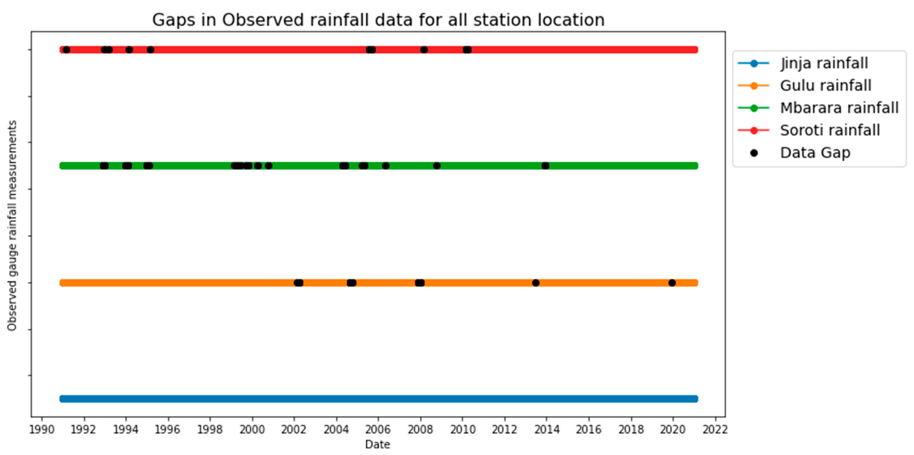
Apart from the Jinja rainfall station, the gauge rainfall observed measurements for the other three stations (Gulu, Soroti, and Mbarara) contained data gaps, ranging from 1 day up to a maximum of 31 days (Figure 5). The percentage of missing rainfall data for the Gulu observed rainfall station was calculated as 0.86%, for the Mbarara station it was 1.80%, and for the Soroti station it was 0.62%, over the 30-year period.

3.1.2. Gaps in Satellite-Based Rainfall Data Products

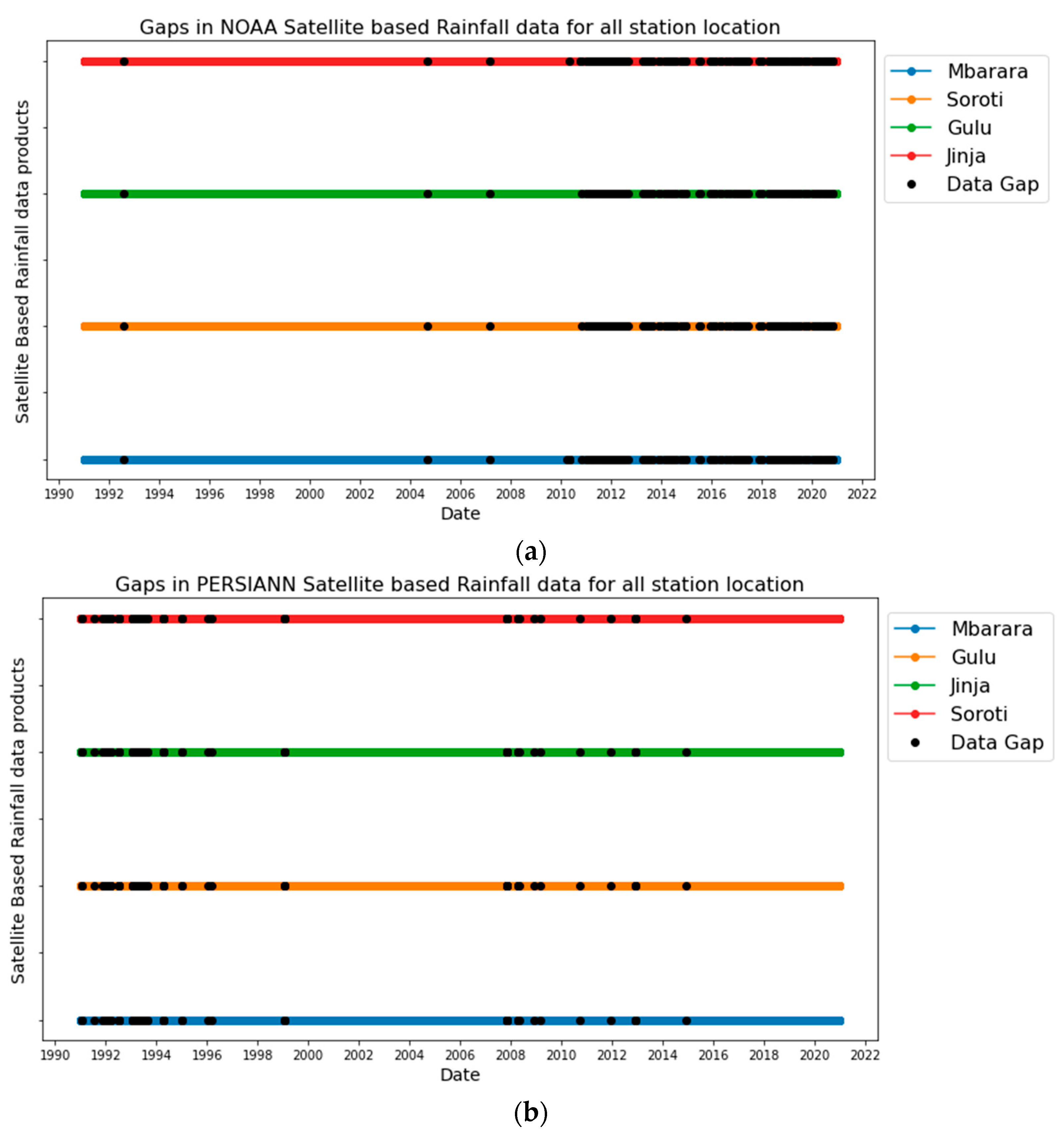
The NOAA_CPC and NOAA_PERSIAAN_CDR satellite datasets exhibited gaps in the rainfall time series for all four rain gauge stations at the Jinja, Mbarara, Soroti, and Gulu locations. The data gaps in the NOAA_CPC rainfall product ranged from 1 to 2 days across all stations during the period of 1991–2020. In the case of PERSIANN_CDR, the data gaps varied from 1 day to a maximum of 29 days (specifically, in February 1992) during the same period (1991–2020) across all stations, as depicted in Figure 6. The percentage of missing rainfall data for the NOAA_CPC remote sensing rainfall product was 1.3%, while for PERSIANN_CDR, it was 0.95% over the 30-year period under consideration. After subjecting all datasets to the quality control procedure, only the NOAA and PERSIANN datasets were found to have gaps in the rainfall data; the rest of the RSR products do not have gaps.

3.1.3. Outlier Test Results

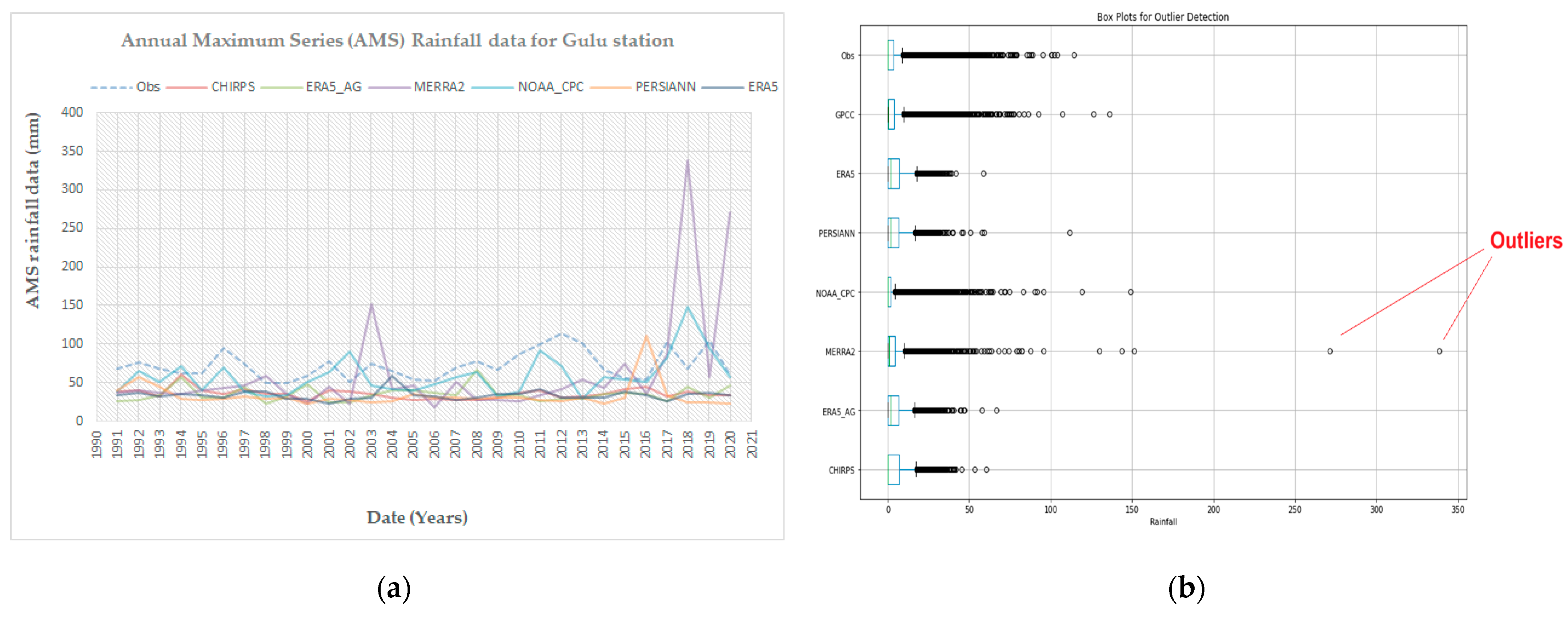
Visual inspections of time series rainfall plots for each station indicated that all four stations were free from outliers except for one RSR product, MERRA2, at the Gulu rainfall station. Applying the IQR method to the same data at the Gulu station confirmed the presence of these outliers in the MERRA2 dataset (Figure 7). The two extreme values identified in the MERRA2 rainfall data were 271.257 mm, recorded on 9 December 2020, and 338.5629 mm, recorded on 27 April 2018. These values were more than 120 mm higher than other rainfall values at the same station. The IQR method (Figure 7b) indicated that almost all rainfall datasets at this station were outliers. However, when applying the IQR methodology alongside other methods, such as visualization from time series plots and pattern comparisons among the datasets (Figure 7a), only the same two values in the MERRA2 datasets were identified as outliers. The rest of the datasets identified as outliers by the IQR method were retained, as they did not appear to be outliers when considering pattern comparisons and simple time series plots. Visualization to identify outliers is not new and has been employed by several authors, including Zhang et al. [43] and Mdegela et al. [44].The only outlier values corrected were for the MERRA2 product, and they were corrected with the 95th-percentile values for the respective years.

3.1.4. Annual Maximum Series Rainfall Data

The AMS rainfall data, extracted from the daily rainfall datasets for all stations, are visually presented in Figure A2 in Appendix A.

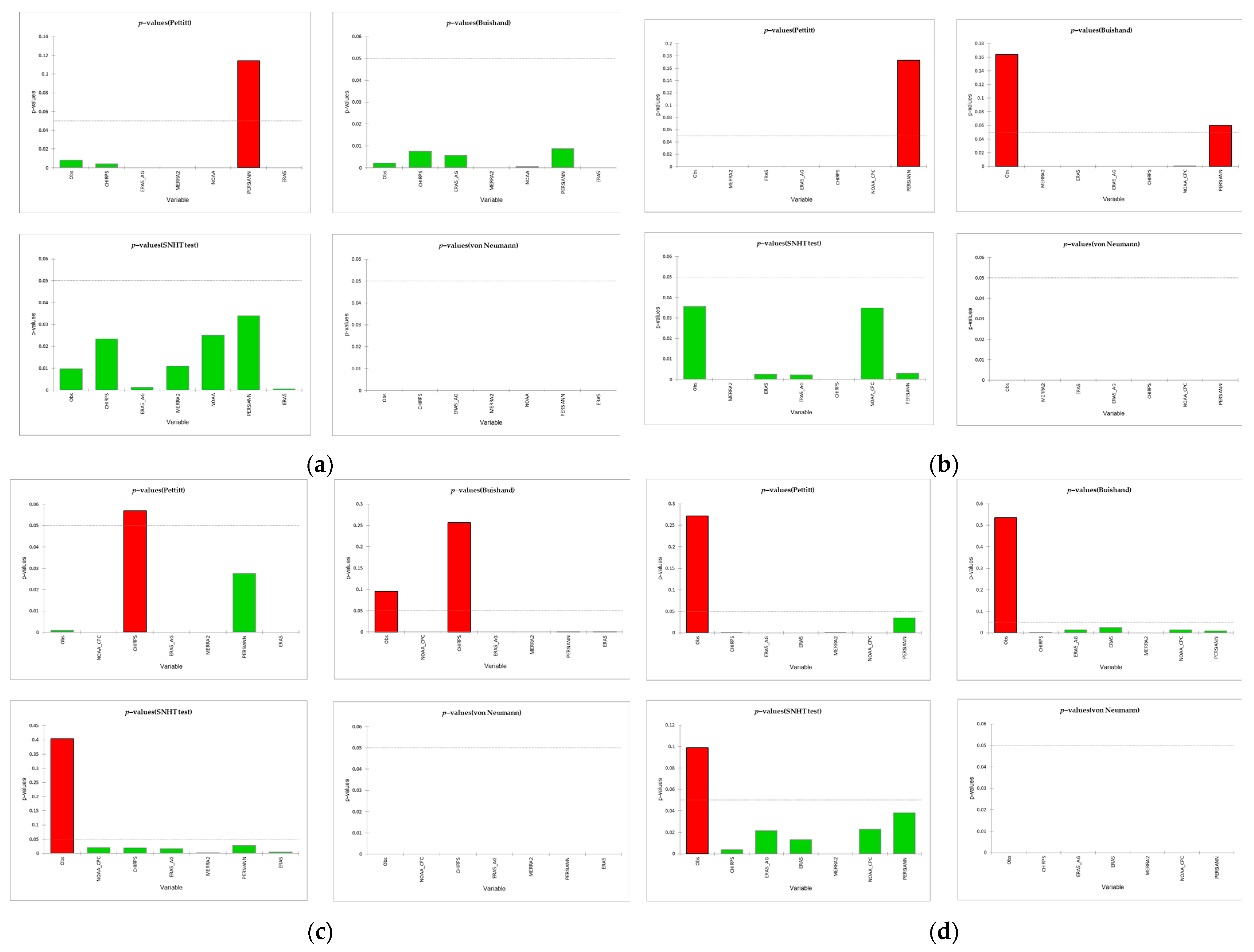
3.1.5. Homogeneity Test Results

Considering the Pettitt homogeneity test method applied to the daily rainfall data, the following results were observed:
  • At the Jinja and Gulu rainfall stations, only the PERSIANN satellite rainfall product exhibits homogeneity, while the remaining satellite and observed rainfall data series demonstrate non-homogeneity.
  • At the Mbarara rainfall station, only the CHIRPS satellite rainfall product displays homogeneity, while the other satellite and observed rainfall data series show non-homogeneity.
  • At the Soroti rainfall station, only the observed rainfall data demonstrate homogeneity, while the other satellite rainfall data products exhibit non-homogeneity.
These results are presented in Table A1, Table A2, Table A3 and Table A4 and Figure A3 in Appendix A.

3.2. Trend Analysis Results

The results of the seasonal and AMS rainfall trend analysis are presented in subsequent sections.

3.2.1. Trends in MAM and SON Seasonal Rainfall

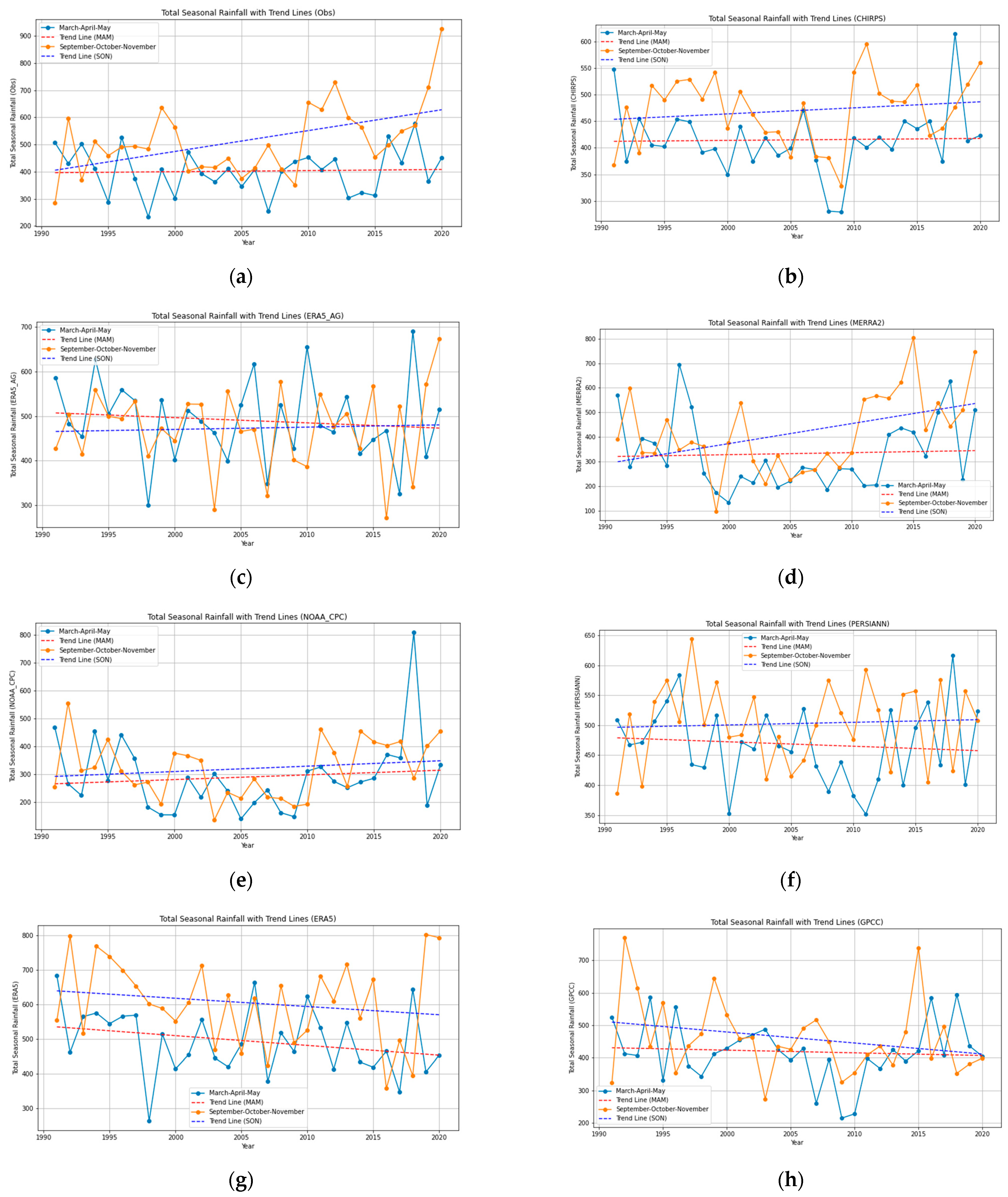
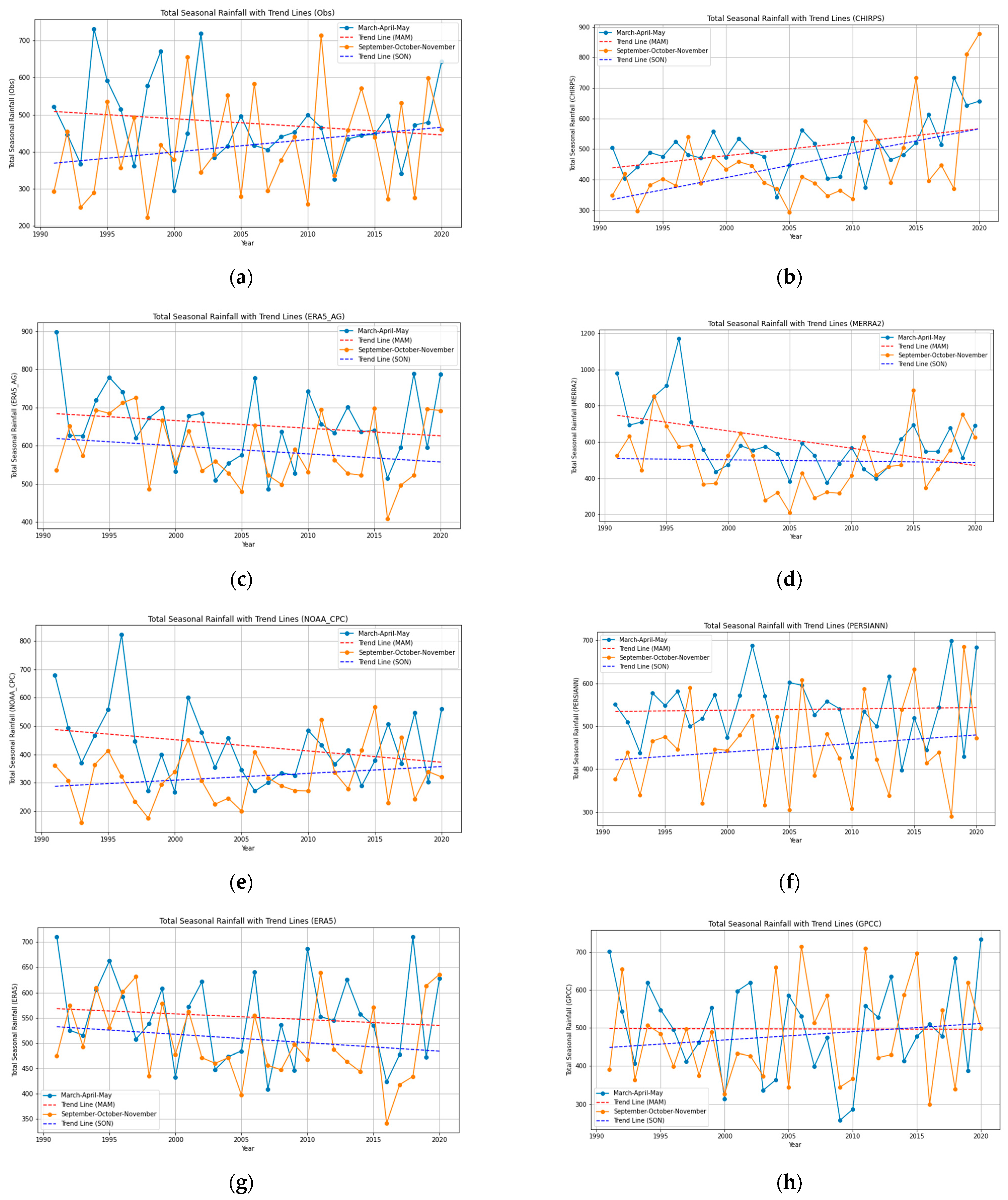
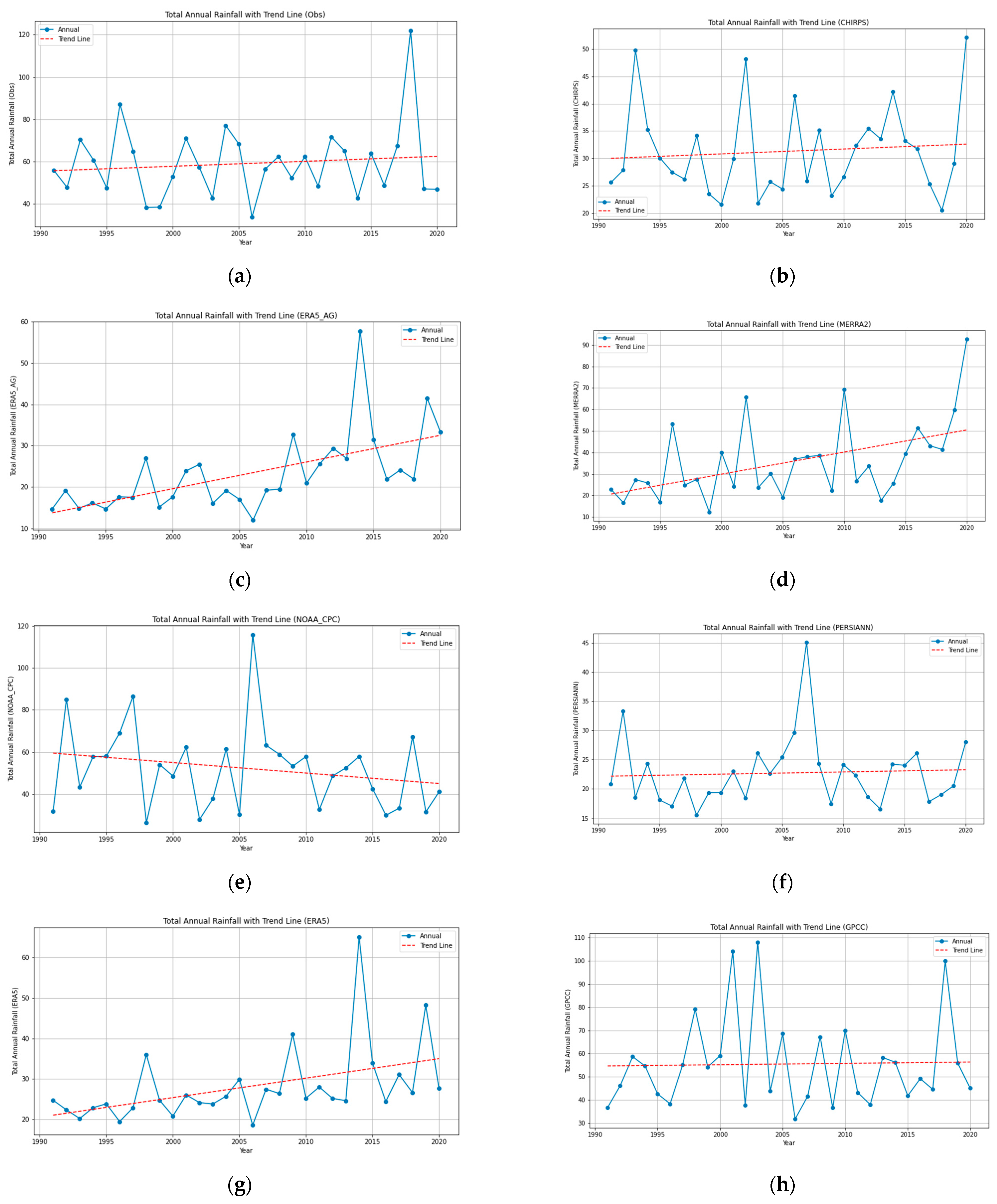
  • At the Gulu rainfall station, the MAM rainfall from observed data show a statistically insignificant increasing trend at a rate of 0.41 mm/year. Similarly, the RSR products, CHIRPS, MERRA2, and NOAA_CPC, show statistically insignificant increasing trends at different rates. The ERA5_AG, ERA5, GPCC, and PERSIANN RSR datasets show a decreasing trend (Table 2).
  • Considering the SON seasonal trends, the observed data show a statistically significant increasing trend at a rate of 7.68 mm/year. The other RSR products that also show increasing trends at different rates are CHIRPS, ERA5_AG, MERRA2, NOAA_CPC, and PERSIANN. The other RSR products (ERA5 and GPCC) show decreasing trends for the SON season.
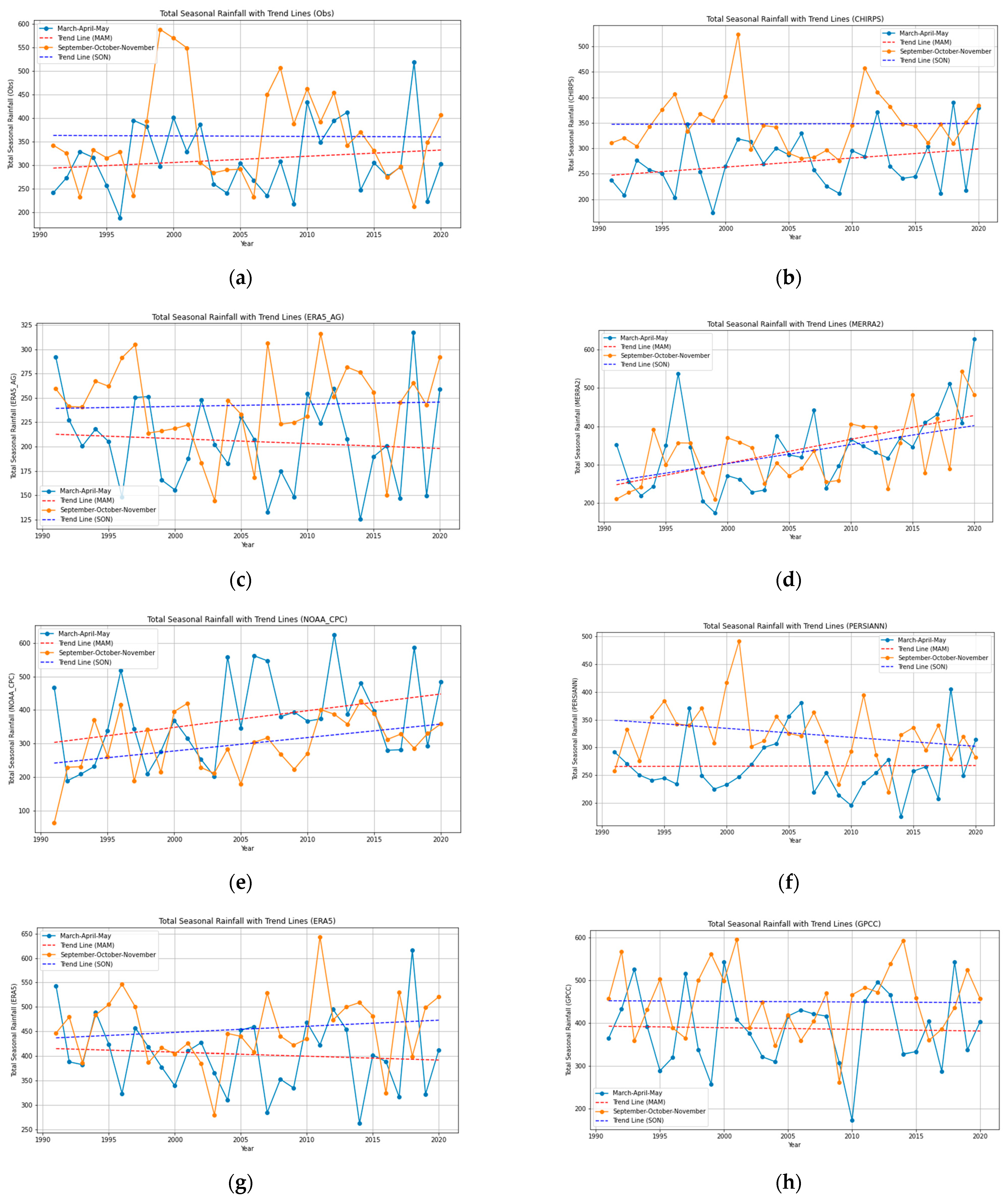
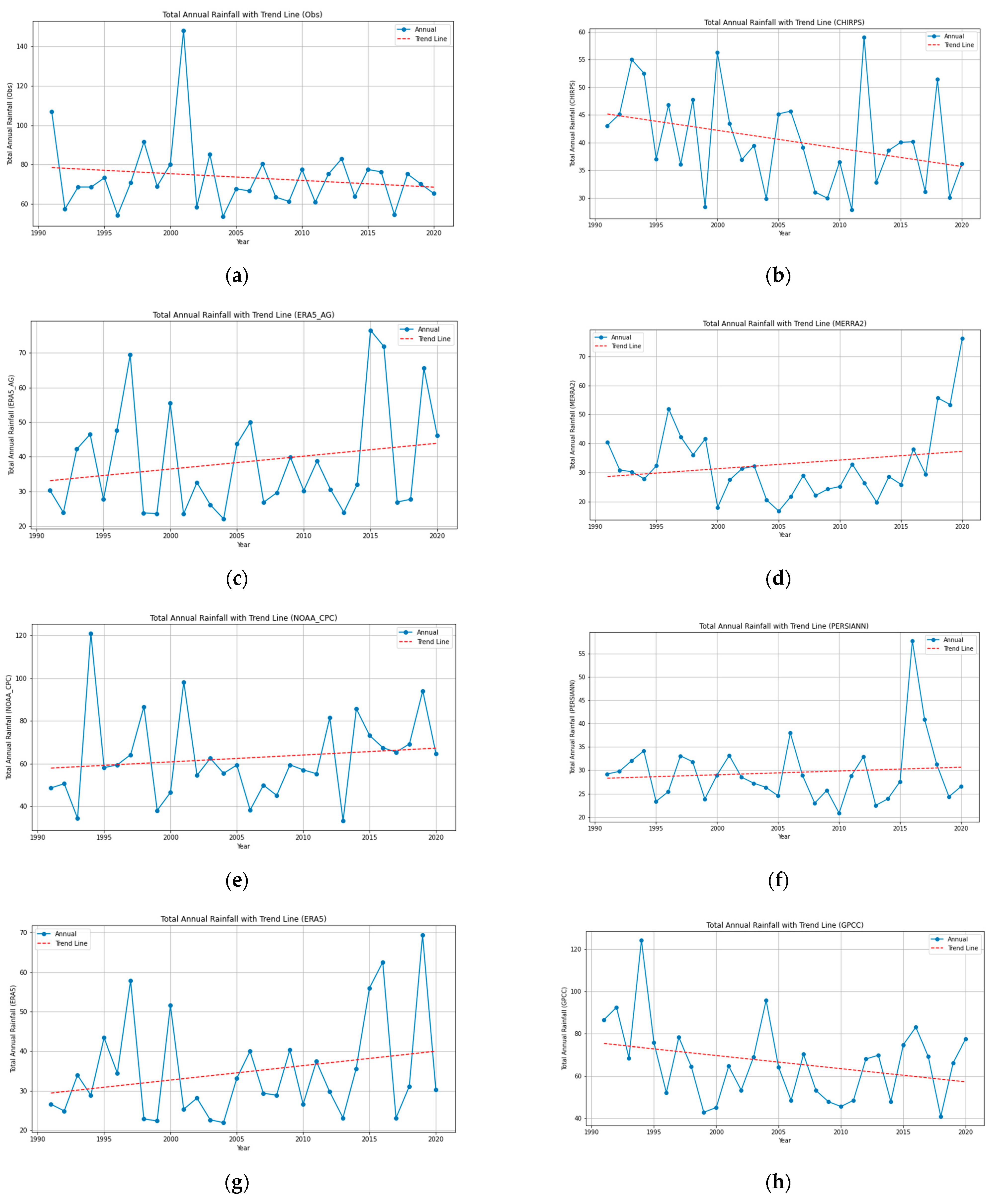
Table 2, Table 3, Table 4 and Table 5 present the MAM and SON seasonal rainfall trend results, which are also illustrated on a map in Figure 8 and in trend graphical plots in Figure A4 and Figure A5 in Appendix A.
Table 2. Trend analysis test results for seasonal rainfall at the Gulu station.
RainfallSeasonTaup-ValueSlope (mm/Year)R2 ValueTrendStatistical Significancy
ObservedMAM0.030.860.410IncreasingNot significant
SON0.290.037.680.26IncreasingSignificant
CHIRPSMAM0.010.940.190IncreasingNot significant
SON0.080.571.140.02IncreasingNot significant
ERA5_AGMAM−0.130.34−1.170.01DecreasingNot significant
SON0.050.70.510IncreasingNot significant
MERRA2MAM0.060.670.820IncreasingNot significant
SON0.250.068.170.2IncreasingNot significant
NOAA_CPCMAM0.060.671.680.01IncreasingNot significant
SON0.110.421.940.03IncreasingNot significant
PERSIANNMAM−0.110.42−0.740.01DecreasingNot significant
SON0.080.570.440IncreasingNot significant
ERA5MAM−0.240.07−2.820.07DecreasingNot significant
SON−0.110.4−2.390.03DecreasingNot significant
GPCCMAM−0.040.75−0.820.01DecreasingNot significant
SON−0.190.14−3.390.07DecreasingNot significant

3.2.2. Trends in AMS Rainfall

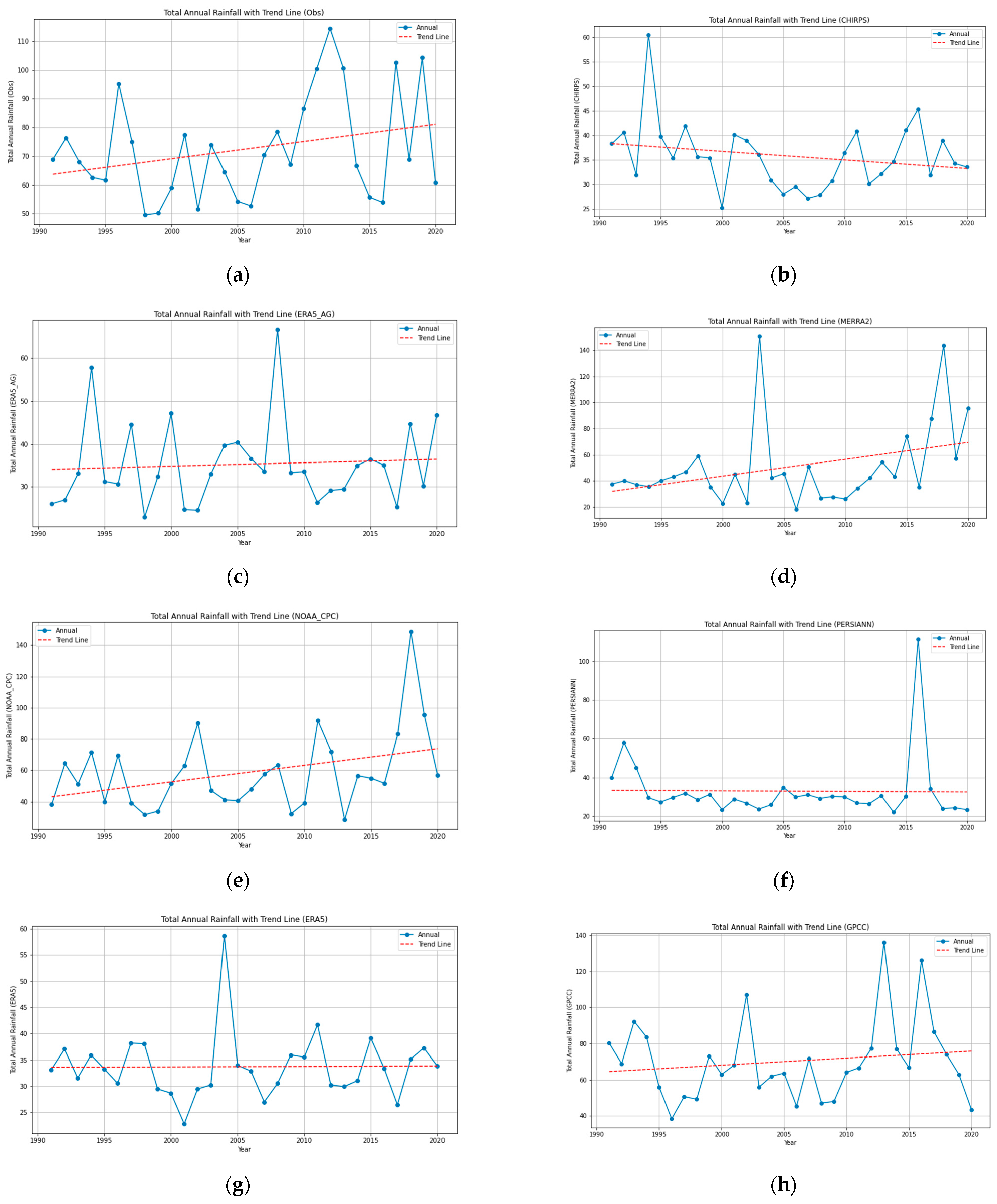
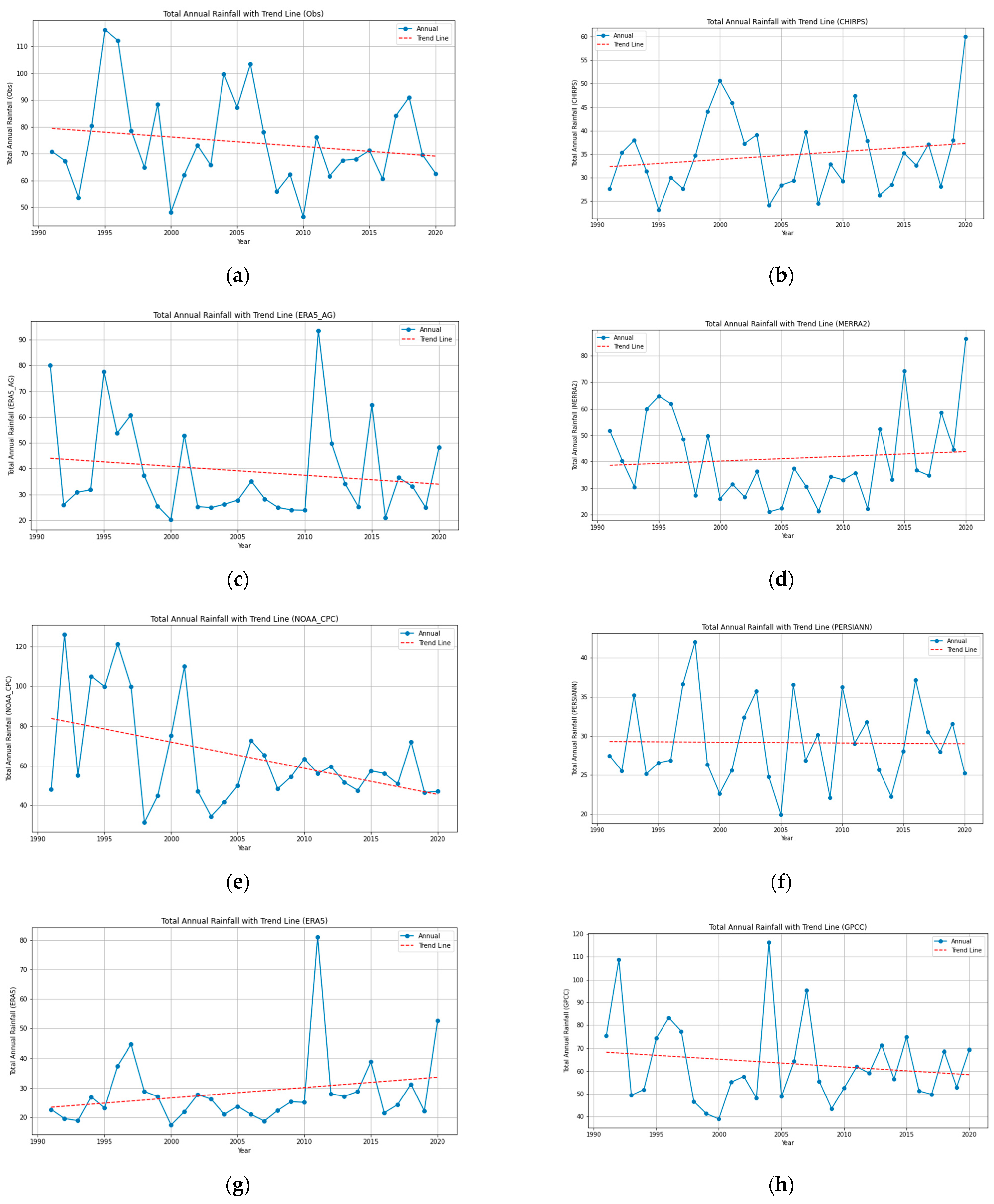
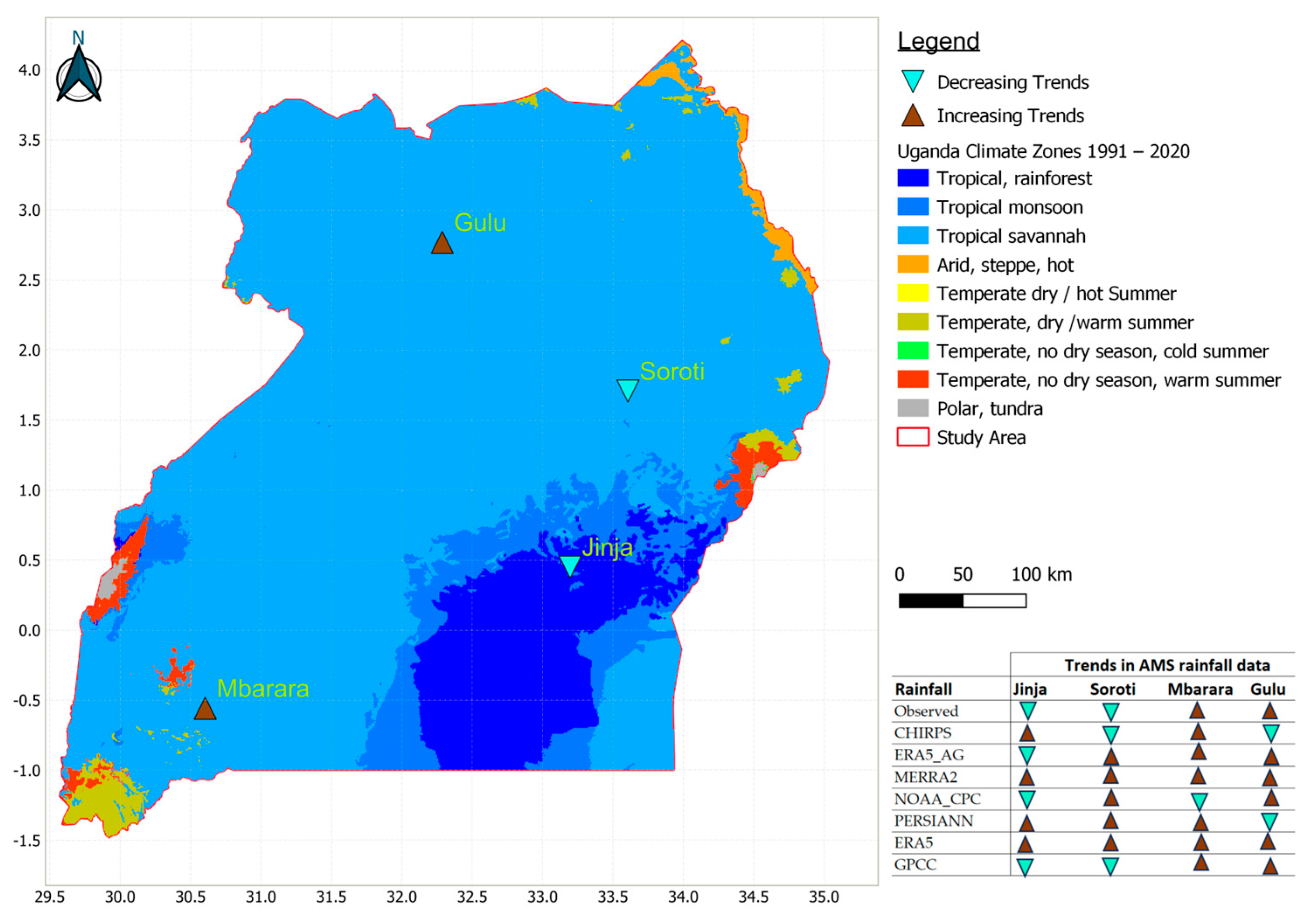
In general, there are statistically insignificant trends in AMS observed rainfall data and in RSR data products at all four stations, except for ERA5_AG and MERRA2, which show statistically significant increasing trends at the Mbarara station. The observed rainfall data at the Gulu and Mbarara stations show that there is a positive increasing trend in the AMS, with rates (Sen slope values) of 0.6 mm/year and 0.23 mm/year, respectively. Conversely, the Soroti and Jinja AMS rainfall data exhibit a negative decreasing trend, with rates (Sen slope values) of −0.34 mm/year and −0.36 mm/year, respectively. Table 6, Table 7, Table 8 and Table 9 show the MK and Sen’s slope trend results and Figure 9 shows a map with different trends at different locations, while in the appendices, Figure A8, Figure A9, Figure A10 and Figure A11 show the graphical trend representation for the AMS rainfall data at the four locations.
The trend analysis conducted on RSR products shows the following results:
  • At the Mbarara station, all RSR products, except NOAA_CPC, exhibit positive increasing trends in AMS rainfall data the same as the observed rainfall.
  • At the Soroti station, only CHIRPS and GPCC display negative decreasing trends in AMS rainfall data the same as the observed rainfall.
  • At the Jinja station, only ERA5_AG, GPCC, and NOAA_CPC display negative decreasing trends in AMS rainfall data the same as the observed rainfall.
  • At the Gulu station, all RSR products, except CHIRPS and PERSIANN, exhibit positive increasing trends the same as the observed rainfall.

3.3. Data Evaluation Results

3.3.1. Results of AMS Variability Analysis

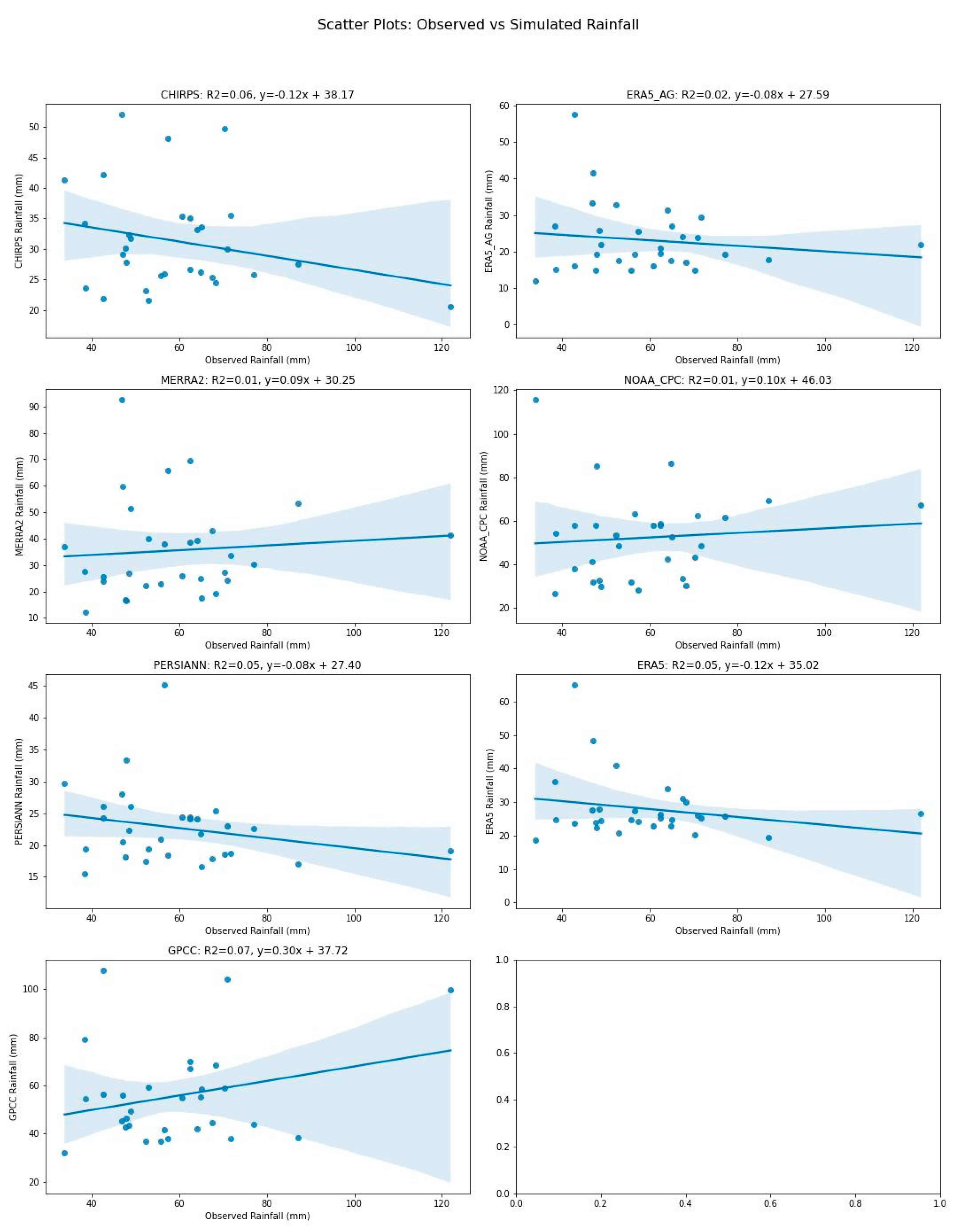
The AMS variability analysis compared the performance of different RSR datasets against observed data, with the results presented in Table 10, Table 11, Table 12 and Table 13 and Figure 10, Figure 11, Figure 12 and Figure 13. The blue shading on the scatter plots shown in Figure 10, Figure 11, Figure 12 and Figure 13 represents the 95% confidence interval (lower and upper bounds) around the regression line. The performance metrics indicate varying degrees of agreement between the observed and RSR data across different locations. In general, for all stations, the negative NSE values for all datasets suggest poor performance, as the observed data significantly deviate from the RSR estimates. Specifically:
  • At the Jinja station, the results show that the GPCC dataset has the highest correlation with observed data (R = 0.41), indicating better performance compared to other datasets.
  • At the Soroti station, the NOAA_CPC (with R = 0.27) performs better compared to the rest of the SRS products.
  • At the Mbarara station, the GPCC dataset has the highest correlation with observed data (R = 0.26), indicating better performance compared to other RSR datasets.
  • At the Gulu station, the NOAA_CPC (with R = 0.30) performed better compared to the rest of the SRS products.
Figure 10. Scatter plots of AMS observed rainfall against the RSR datasets for the Jinja station.
Sustainability 16 06081 g010
Figure 11. Scatter plots of AMS observed rainfall against the RSR datasets for the Soroti station.
Sustainability 16 06081 g011
Figure 12. Scatter plots of AMS observed rainfall against the RSR datasets for the Mbarara station.
Sustainability 16 06081 g012
Figure 13. Scatter plots of AMS observed rainfall against the RSR datasets for the Gulu station.
Sustainability 16 06081 g013
Table 10. Results of the performance metrics tests on AMS rainfall at the Jinja station.
RainfallRMSEMAERR2NRMSEPBIASNSESDCoV
CHIRPS45.0939.64−0.380.140.61−53.18−5.908.400.24
ERA5_AG41.3037.040.300.090.56−47.51−4.7919.080.49
MERRA238.5234.870.300.090.52−44.57−4.0416.250.39
NOAA_CPC27.6323.420.300.090.37−12.93−1.5925.230.39
PERSIANN48.8845.10−0.180.030.66−60.76−7.115.310.18
ERA550.0446.030.080.010.67−61.57−7.5012.390.43
GPCC22.2217.560.410.170.30−14.64−0.6818.540.29
Table 11. Results of the performance metrics tests on AMS rainfall at the Soroti station.
RainfallRMSEMAERR2NRMSEPBIASNSESDCoV
CHIRPS37.6733.070.230.050.51−45.00−3.398.5937.67
ERA5_AG43.3035.02−0.150.020.59−47.65−4.8015.6143.30
MERRA246.4141.27−0.060.000.63−55.16−5.6712.6846.41
NOAA_CPC25.2419.030.270.070.34−14.79−0.9719.5725.24
PERSIANN47.8044.020.100.010.65−59.89−6.076.9647.80
ERA545.0238.76−0.090.010.61−52.74−5.2812.6245.02
GPCC26.0818.910.040.000.35−9.66−1.1118.2926.08
Table 12. Results of the performance metrics tests on AMS rainfall at the Mbarara station.
RainfallRMSEMAERR2NRMSEPBIASNSESDCoV
CHIRPS34.5628.61−0.240.060.59−46.99−3.138.230.26
ERA5_AG41.3636.94−0.140.020.70−60.85−4.929.270.40
MERRA233.3528.830.080.010.56−39.85−2.8517.910.50
NOAA_CPC25.7719.510.090.010.44−11.63−1.3019.700.38
PERSIANN41.1036.33−0.230.050.70−61.51−4.845.840.26
ERA537.4832.59−0.220.050.63−52.53−3.869.210.33
GPCC22.6216.600.260.070.38−5.93−0.7719.630.35
Table 13. Results of the performance metrics tests on AMS rainfall at the Gulu station.
RainfallRMSEMAERR2NRMSEPBIASNSESDCoV
CHIRPS41.6436.62−0.120.020.58−50.59−4.456.730.19
ERA5_AG43.2737.14−0.230.050.60−51.32−4.899.790.28
MERRA240.7536.060.090.010.56−30.01−4.2231.140.61
NOAA_CPC29.2022.440.300.090.40−19.23−1.6824.690.42
PERSIANN47.3043.28−0.180.030.65−54.50−6.0316.180.49
ERA543.2938.66−0.110.010.60−53.41−4.896.180.18
GPCC27.4621.150.080.010.38−3.05−1.3722.280.32

3.3.2. Goodness-of-Fit Test Results

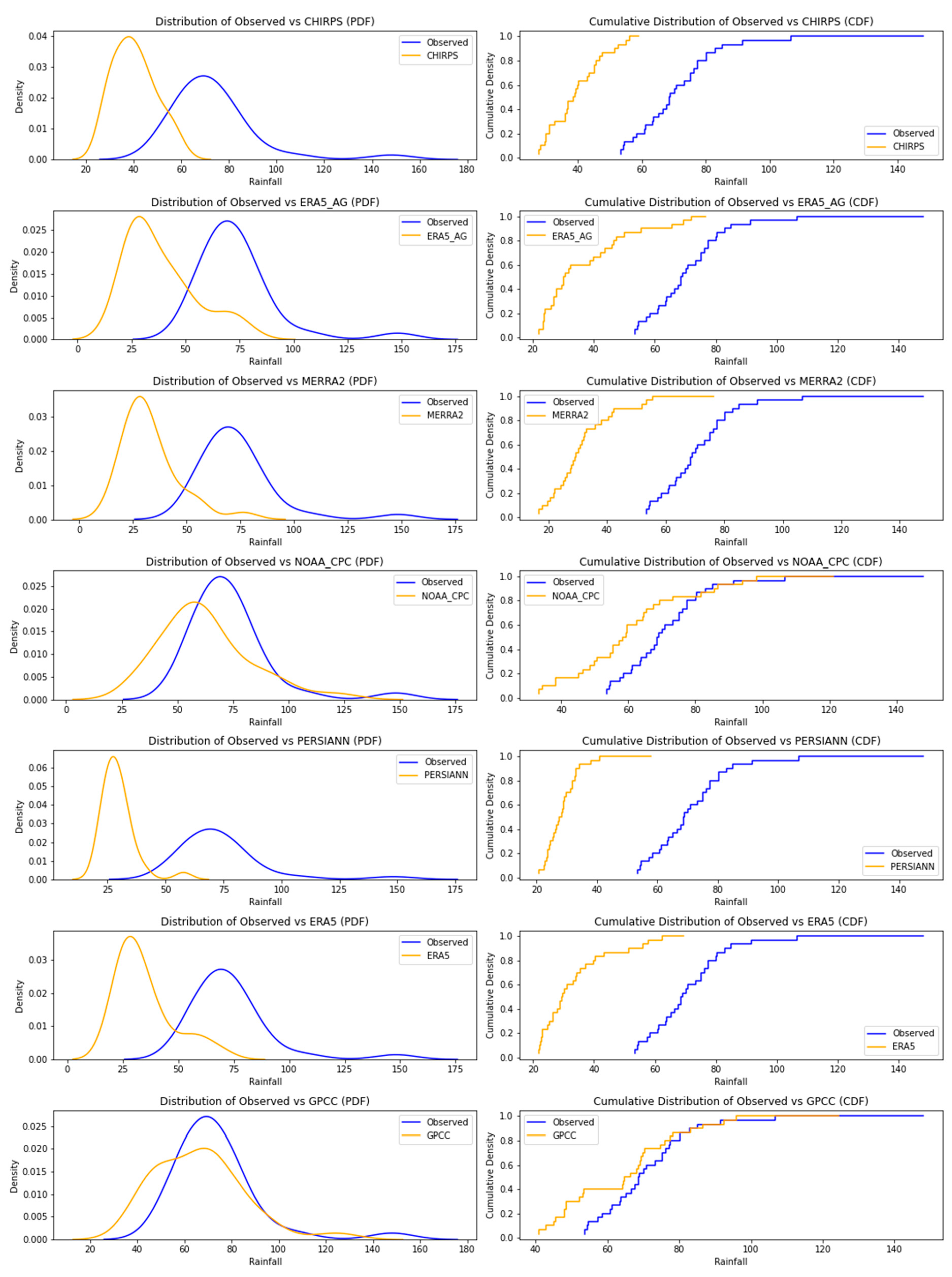
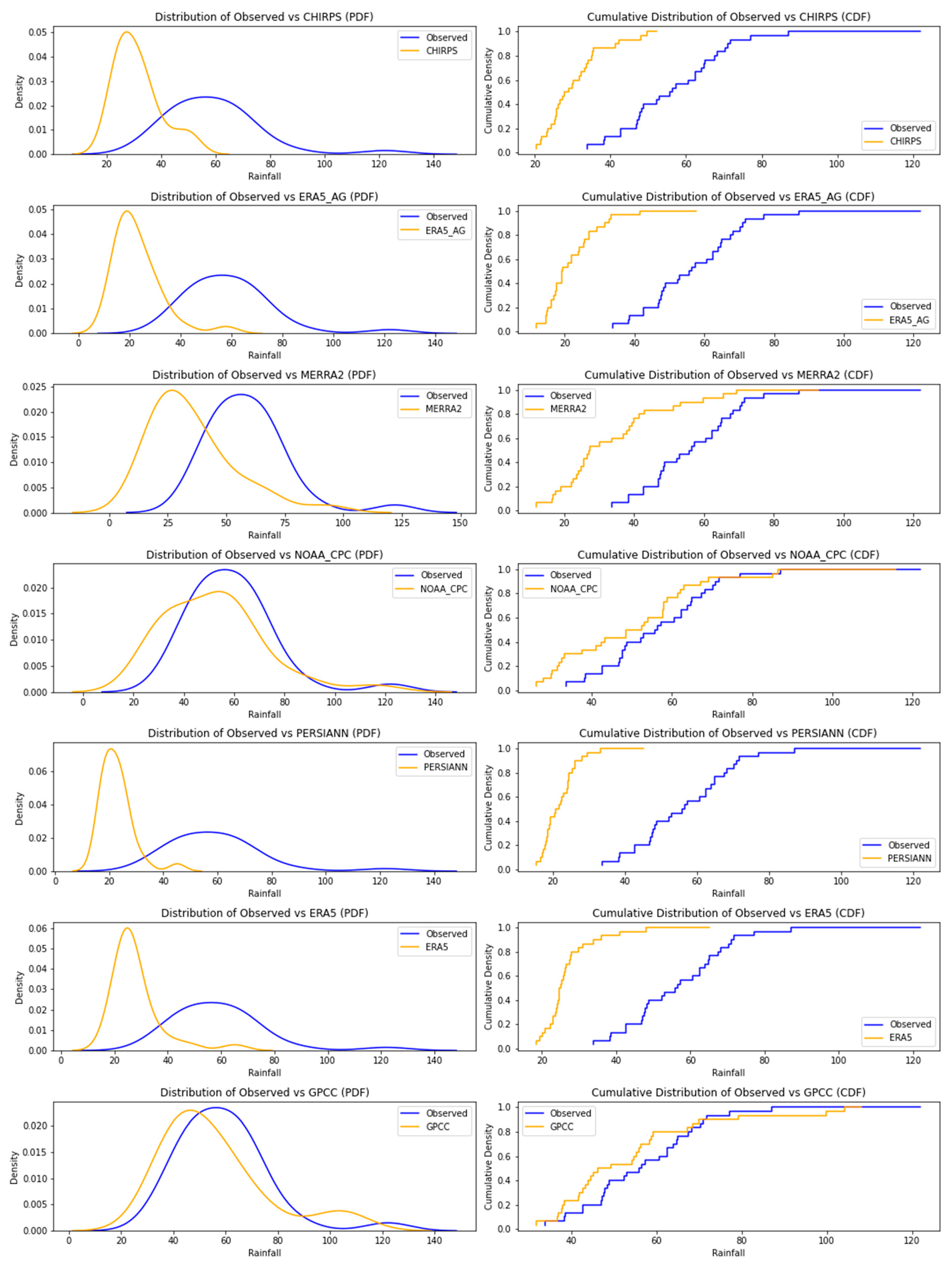
The Kolmogorov–Smirnov test results indicated significant differences in the distribution of the observed data compared to most RSR datasets, as shown in Table 14 and Figure 11, Figure 12, Figure 13 and Figure 14.
  • At the Jinja station, the goodness-of-fit test results show that the GPCC RSR data product, with a KS value of 0.43, outperforms all other products. However, the p-value is less than the 5% significance level, indicating a poor fit.
  • Similarly, at the Soroti station, the fit between the observed data and the other RSR products is also poor (p-value less than 5%), although the GPCC product is relatively better with a lower KS value of 0.37.
  • At the Gulu and Mbarara stations, the KS test results show a significant agreement between the GPCC dataset and the observed rainfall data, outperforming the other RSR products. The KS p-values for the GPCC distribution against the observed rainfall at the Gulu and Mbarara stations were 0.60 and 0.14, respectively. This suggests that the GPCC data are the most comparable to the observed data in terms of distribution, whereas other datasets exhibit significant biases. Another product that showed a good fit with the observed data distribution is NOAA_CPC, with a p-value of 0.24 at the Mbarara station.
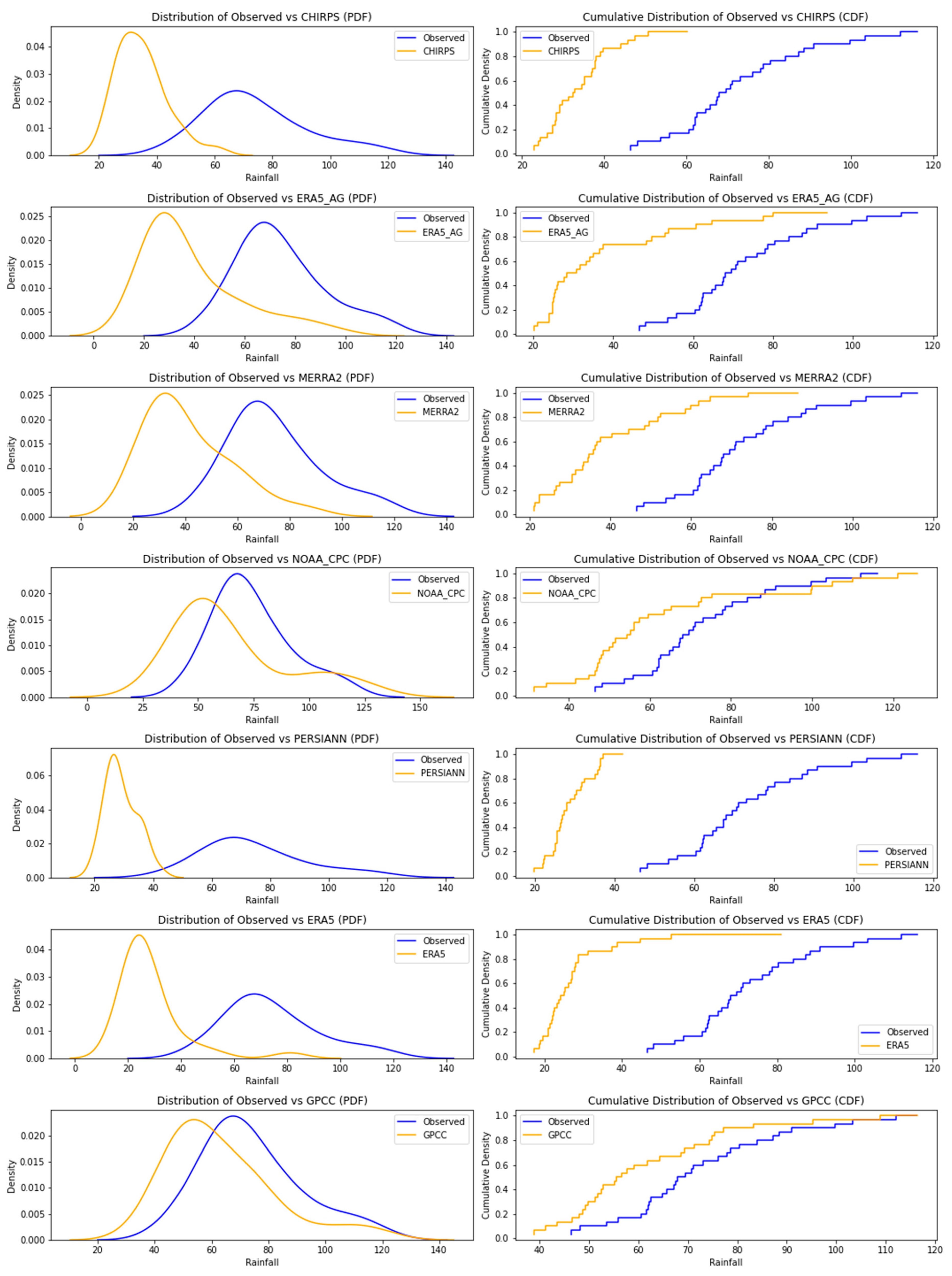
Table 14 and Figure 14, Figure 15, Figure 16 and Figure 17 provide the KS statistics and p-values for the distributions of the RSR datasets compared to the observed data distribution.
Figure 14. PDF and CDF of distributions of the observed AMS and RSR dataset at the Jinja station.
Sustainability 16 06081 g014
Table 14. Goodness-of-fit test results for all stations.
Jinja StationSoroti StationMbarara StationGulu Station
RainfallKSp-ValueKSp-ValueKSp-ValueKSp-Value
CHIRPS0.900.000.900.000.800.000.970.00
ERA5_AG0.730.000.830.000.930.000.930.00
MERRA20.730.000.930.000.670.000.700.00
NOAA_CPC0.500.000.400.020.270.240.400.02
PERSIANN1.000.000.970.000.970.000.930.00
ERA50.930.000.870.000.870.000.970.00
GPCC0.430.010.370.030.300.140.200.60

4. Discussion

4.1. Trends in Seasonal and AMS Rainfall Data

The results of the seasonal and AMS rainfall trend analysis across the four rainfall stations revealed both increasing and decreasing trends. Most of these trends were statistically insignificant, as the computed p-values were above the 5% significance level.
Notably, the SON seasonal rainfall trend at the Gulu station was statistically significant (p-value = 0.03), with an increasing rate of 7.68 mm/year. This increase in SON rainfall aligns with previous studies on rainfall trends in tropical regions, where shifts in seasonal rainfall patterns have been observed. For instance, Nsubuga et al. [10] reported increasing SON seasonal rainfall across all four subbasins in Uganda. The World Bank [2] also noted an increase in SON seasonal rainfall in northern Uganda, specifically in the Gulu region. Additionally, Majaliwa et al. [11] observed similar increasing trends in SON seasonal rainfall in northern Uganda.
Regarding AMS rainfall trends, the observed rainfall at all four stations displays insignificant increasing (at the Gulu and Mbarara rainfall stations) and decreasing trends (at the Jinja rainfall station). Similarly, all RSR products show insignificant trends, except for MERRA2 and ERA5_AG, which exhibit statistically significant increasing trends at the Mbarara station. While the trend analysis on the AMS showed no statistically significant increasing trends, the World Bank report indicated increased flooding in Uganda [2]. Based on the findings of this research, the increased flooding incidents may not be attributed to increasing trends in the AMS but are probably due to increased rainfall intensities.

4.2. Variability of Observed AMS and RSR Products

The AMS variability analysis based on statistical metrics (RMSE, MAE, R, R2, NRMSE, PBIAS, NSE, SD, and CoV) shows varying degrees of agreement between the RSR data and observed data across different station locations. Considering the negative NSE values, all the RSR datasets suggest poor performance at all four stations considered in this study.
Considering the PBIAS performance metric, the GPCC and NOAA_CPC data products outperform other RSR data products. In hydrological applications, PBIAS values of less than ±10% are considered very good performance, ±10% to ±15% indicate good performance, and ±15% to ±25% indicate fair performance according to Moriasi et al. [45]. Therefore, based on the PBIAS performance metric, the best products are as follows:
  • At the Jinja station location (tropical rainforest climate zone), the best performing product is NOAA_CPC with a PBIAS value of −12.93%, followed by GPCC with a PBIAS value of −14.64%.
  • At the Soroti station location (tropical savannah climate zone in eastern Uganda), the best performing product is GPCC with a PBIAS value of −9.66%, followed by NOAA_CPC with a PBIAS value of −14.79%.
  • At the Mbarara station location (tropical savannah climate zone in southwest Uganda), the best performing product is GPCC with a PBIAS value of −5.93%, followed by NOAA_CPC with a PBIAS value of −11.63%.
  • At the Gulu station location (tropical savannah climate zone in northern Uganda), the best performing product is GPCC with a PBIAS value of −3.05%, followed by NOAA_CPC with a PBIAS value of −19.23%.
In general, the statistical performance metrics highlight the challenges in accurately capturing AMS rainfall using RSR datasets, as each metric tends to favor different products. However, based on the PBIAS metric, this research reveals identifiable patterns in the variability of GPCC and NOAA_CPC AMS rainfall data comparable to observed AMS rainfall data, with GPCC and NOAA_CPC outperforming other RSR datasets at all four locations.
In the region, Macharia et al. [13] evaluated the performance of various RSR products (CHIRPS, GPCC, MERRA, and others) in neighboring country Kenya, determining their suitability for use in the eight agro-ecological zones of Kenya based on monthly temporal resolutions. Similarly, other studies by Nsubuga et al. [10] and Majaliwa et al. [11] also used monthly timesteps for their analyses. In contrast, our research employed higher temporal resolution (daily timestep) datasets to identify suitable RSR products for hydrological infrastructure design in different climatic regions of Uganda.

4.3. Distribution of RSR Data Compared to Observed AMS Rainfall Data

The Kolmogorov–Smirnov test results indicate significant differences in the RSR data distributions compared to the observed data distribution. However, at the Gulu and Mbarara stations, the KS test results show significant agreement between the GPCC dataset and the observed rainfall data, with KS p-values of 0.60 and 0.14, respectively. Another well-performing product based on the KS test is NOAA_CPC, which demonstrates a good fit with observed data at the Mbarara station, with a p-value of 0.24. In fact, at the Mbarara station, NOAA_CPC is the best-performing RSR product.
The good agreement of the GPCC and NOAA_CPC products with observed data based on KS test results, particularly at the Gulu and Mbarara stations, suggests that they could be viable alternatives for use in areas without observed data for hydrological applications. Despite lower p-values at the Jinja and Soroti locations, the GPCC dataset still outperforms other RSR products. Thus, in regions lacking observed data, the GPCC dataset offers a reliable alternative for hydrological studies.

5. Conclusions

This research aimed to analyze the trends and variability of the AMS and seasonal rainfall data in Uganda, comparing observed data with various RSR products.

5.1. Trends in Seasonal and AMS Rainfall Data

The results of the seasonal and AMS rainfall trend analysis across the four rainfall stations show both increasing and decreasing trends. However, most of these trends are statistically insignificant, as the computed p-values exceed the 5% significance level.
For seasonal rainfall, only the SON observed rainfall trends at the Gulu station is statistically significant (p-value = 0.03), with an increasing rate of 7.68 mm/year. This finding aligns with previous studies (such as the World Bank [2], Nsubuga et al. [10], and Majaliwa et al. [11]) indicating an increase in the SON season rainfall in northern Uganda.
The rest of the trends (both increasing and decreasing) in RSR data products at the Gulu station are statistically insignificant. Similarly, the trends in seasonal observed rainfalls (both increasing and decreasing) at the other three stations (Soroti, Jinja, and Mbarara) are also statistically insignificant. At the Jinja and Soroti stations, the MAM rainfall shows decreasing trends of −2.17 mm/year and −2.17 mm/year, respectively, while SON rainfall shows increasing trends of 3.34 mm/year and 1.28 mm/year, respectively. At the Mbarara station, the MAM season observed rainfall shows increasing trends at a rate of 1.32 mm/year, while SON season rainfall shows decreasing trends at a rate of −0.11 mm/year.
At all four stations, there are statistically insignificant trends in AMS observed rainfall data and in RSR data products, except for ERA5_AG and MERRA2, which show statistically significant increasing trends at the Mbarara station. The observed rainfall data at the Gulu and Mbarara stations show that there is a positive increasing trend in the AMS, with rates of 0.6 mm/year and 0.23 mm/year, respectively. Conversely, the Soroti and Jinja AMS observed rainfall data exhibit a negative decreasing trend, with rates of −0.34 mm/year and −0.36 mm/year, respectively.
This study reveals several statistically significant trends in rainfall data:
  • At the Gulu station, there are statistically significant increasing trends in observed SON season rainfall.
  • At the Mbarara station, MERRA2 and NOAA_CPC RSR data show statistically significant increasing trends for both MAM and SON seasons.
  • At the Jinja station, CHIRPS rainfall product shows statistically significant increasing trends for the MAM season, while MERRA2 rainfall product shows statistically significant decreasing trends for the MAM season.
  • Only the ERA5_AG and MERRA2 datasets exhibit statistically significant increasing trends in AMS rainfall data at the Mbarara station.
These statistically significant trends address the hypotheses about the significance of trends in seasonal and AMS rainfall data. The significant increasing trends in seasonal rainfall suggest the need for strategic planning to adapt to increasing SON seasonal rainfall. Regarding AMS observed rainfall data, there are no statistically significant trends, indicating that AMS trends may not adequately inform hydrological infrastructure design. Further research is needed to determine whether the insignificant increasing trends in observed AMS rainfall data could impact hydrological infrastructure design.

5.2. Variability in AMS Rainfall Data

The variability in AMS rainfall data based on statistical performance metrics (RMSE, MAE, R, R2, NRMSE, PBIAS, NSE, SD, and CoV) shows varying degrees of agreement between the RSR data and observed data across the four station locations. Considering the negative NSE values, all the RSR datasets suggest poor performance at the four stations analyzed in this study. However, based on the PBIAS performance metric, the GPCC and NOAA_CPC data products outperform other RSR datasets. The performance based on the PBIAS metric is as follows:
  • At the Jinja station (tropical rainforest climate zone), NOAA_CPC performs best with a PBIAS value of −12.93%, followed by GPCC with a PBIAS value of −14.64%.
  • At the Soroti station (tropical savannah climate zone in eastern Uganda), GPCC performs best with a PBIAS value of −9.66%, followed by NOAA_CPC with a PBIAS value of −14.79%.
  • At the Mbarara station (tropical savannah climate zone in southwest Uganda), GPCC performs best with a PBIAS value of −5.93%, followed by NOAA_CPC with a PBIAS value of −11.63%.
  • At the Gulu station (tropical savannah climate zone in northern Uganda), GPCC performs best with a PBIAS value of −3.05%, followed by NOAA_CPC with a PBIAS value of −19.23%.
Overall, the statistical performance metrics highlight the challenges in accurately capturing AMS rainfall using RSR datasets, as each metric tends to favor different products. However, based on the PBIAS metric, this research reveals identifiable patterns in the variability of GPCC and NOAA_CPC AMS rainfall data comparable to observed AMS rainfall data, with GPCC and NOAA_CPC outperforming other RSR datasets at all four locations.

5.3. Distribution of RSR Data Compared to Observed Rainfall Data Distribution

The Kolmogorov–Smirnov test results indicate significant differences in the RSR data distributions compared to the observed data distribution, except for GPCC and NOAA_CPC at the Gulu and Mbarara stations. At these stations, the GPCC dataset shows significant agreement with the observed data, with KS p-values of 0.60 and 0.14, respectively. Another well-performing product based on the KS test is NOAA_CPC, which shows a good fit with the observed data at the Mbarara station, with a p-value of 0.24.
Overall, the GPCC RSR product outperforms other RSR products at the Gulu, Soroti, and Jinja stations based on the goodness-of-fit test results, while at the Mbarara station, the NOAA_CPC rainfall data outperform other RSR products based on the same test.

5.4. Research Limitations

One of the primary limitations of this study is the potential uncertainty inherent in both observed and RSR data. Observed data, while generally accurate, can suffer from inconsistencies due to equipment malfunctions, human error in data recording, and incomplete datasets, evidenced by the homogeneity tests performed. Despite our efforts to fill gaps using linear interpolation and other methods, some residual inaccuracies may persist. Similarly, to observed data, RSR datasets also have gaps (PERSIANN and NOAA_CPC datasets at all four stations) and anomalies (MERRA2 at the Gulu station). These issues can introduce additional uncertainty into the trend and variability analysis.

5.5. Potential Areas for Further Studies

The potential areas for further studies are:
  • Investigating the frequency and intensity of extreme weather events, such as droughts and storms, and their correlation with rainfall trends can provide deeper insights into climate variability and its impact on hydrological systems.
  • Assessing the long-term impacts of identified trends on water resources, agriculture, and urban infrastructure will be of great value. This could involve hydrological modeling to simulate the effects of changing rainfall patterns on river flows, groundwater recharge, and flood risks.

5.6. Principal Conclusions

This research highlights the limitations of current RSR datasets in accurately replicating observed AMS rainfall data and proposes viable alternatives for use in areas lacking observed data. In general, GPCC and NOAA_CPC products are identified as suitable alternatives for all the Gulu, Soroti, Jinja, and Mbarara stations, outperforming other RSR products based on the PBIAS metric. Based on KS test results, GPCC is identified as the better product for hydrological applications at the Gulu, Jinja, and Soroti station areas. For the Mbarara station, NOAA_CPC outperforms other RSR products based on the goodness-of-fit test.

Author Contributions

Conceptualization, M.O.; methodology, M.O.; software, M.O.; validation, M.O. and J.D.P.; formal analysis, M.O. and J.D.P.; investigation, M.O. and J.D.P.; resources, M.O. and J.D.P.; data curation, M.O.; writing—original draft preparation, M.O.; writing—review and editing, M.O. and J.D.P.; visualization, M.O. and J.D.P.; supervision, J.D.P.; project administration, J.D.P.; funding acquisition, M.O. and J.D.P. All authors have read and agreed to the published version of this manuscript.

Funding

This research received no external funding.

Institutional Review Board Statement

Not applicable.

Informed Consent Statement

Not applicable.

Data Availability Statement

The Uganda National Meteorological Authority (UNMA) provided the observed daily rainfall data for the four rain gauge stations. The observed daily rainfall raw data supporting the conclusions of this article will be made available by the authors on request. The satellite-based rainfall data presented in this research is openly available at https://app.climateengine.com/climateEngine, accessed on 16 December 2022.

Acknowledgments

The authors wish to greatly appreciate the anonymous peer reviewers from Sustainability MDPI journal for their valuable inputs and suggestions to the article.

Conflicts of Interest

The authors declare no conflicts of interest.

Appendix A

Figure A1. Double Mass Curve (DMC) plots depicting cumulative PERSIANN rainfall data (in millimeters) against cumulative NOAA rainfall data for the following four stations: (a) Gulu rainfall station, (b) Jinja rainfall station, (c) Mbarara rainfall station, and (d) Soroti rainfall station.
Sustainability 16 06081 g0a1
Figure A2. Annual Maximum Series rainfall data extracted from daily rainfall data for the following stations: (a) Gulu rainfall station, (b) Jinja rainfall station, (c) Mbarara rainfall station, and (d) Soroti rainfall station.
Sustainability 16 06081 g0a2aSustainability 16 06081 g0a2b
Figure A3. Homogeneity test p–values on daily rainfall data for the following stations: (a) Gulu rainfall station, (b) Jinja rainfall station, (c) Mbarara rainfall station, and (d) Soroti rainfall station.
Sustainability 16 06081 g0a3
Table A1. Homogeneity test computed p-values for daily rainfall products at the Gulu station.
Rainfall ProductsPettittSNHT TestBuishandvon Neumann
Observed0.0080.0100.002<0.0001
CHIRPS0.0040.0230.008<0.0001
ERA5_AG<0.00010.0010.006<0.0001
MERRA2<0.00010.011<0.0001<0.0001
NOAA<0.00010.0250.001<0.0001
PERSIANN0.1140.0340.009<0.0001
ERA5<0.00010.001<0.0001<0.0001
Table A2. Homogeneity test computed p-values for daily rainfall products at the Jinja station.
Rainfall ProductsPettittSNHT TestBuishandvon Neumann
Observed<0.00010.0360.164<0.0001
MERRA2<0.0001<0.0001<0.0001<0.0001
ERA5<0.00010.003<0.0001<0.0001
ERA5_AG<0.00010.002<0.0001<0.0001
CHIRPS<0.0001<0.0001<0.0001<0.0001
NOAA_CPC<0.00010.0350.001<0.0001
PERSIANN0.1730.0030.060<0.0001
Table A3. Homogeneity test computed p-values for daily rainfall products at the Mbarara station.
Rainfall ProductsPettittSNHT TestBuishandvon Neumann
Observed0.0010.4040.096<0.0001
NOAA_CPC<0.00010.020<0.0001<0.0001
CHIRPS0.0570.0190.257<0.0001
ERA5_AG<0.00010.016<0.0001<0.0001
MERRA2<0.00010.001<0.0001<0.0001
PERSIANN0.0280.0290.000<0.0001
ERA5<0.00010.0040.000<0.0001
Table A4. Homogeneity test computed p-values for daily rainfall products at the Soroti station.
Rainfall ProductsPettittSNHT TestBuishandvon Neumann
Observed0.2710.0990.535<0.0001
CHIRPS0.0010.0040.003<0.0001
ERA5_AG<0.00010.0220.015<0.0001
ERA5<0.00010.0130.024<0.0001
MERRA20.000<0.0001<0.0001<0.0001
NOAA_CPC<0.00010.0230.014<0.0001
PERSIANN0.0350.0380.009<0.0001
Figure A4. MAM and SON seasonal rainfall trend analysis results at the Gulu station: (a) Observed data, (b) CHIRPS, (c) ERA5_AG, (d) MERRA2, (e), NOAA_CPC, (f) PERSIANN, (g) ERA5, and (h) GPCC.
Sustainability 16 06081 g0a4
Figure A5. MAM and SON seasonal rainfall trend analysis results at the Jinja station: (a) Observed data, (b) CHIRPS, (c) ERA5_AG, (d) MERRA2, (e), NOAA_CPC, (f) PERSIANN, (g) ERA5, and (h) GPCC.
Sustainability 16 06081 g0a5
Figure A6. MAM and SON seasonal rainfall trend analysis results at the Mbarara station: (a) Observed data, (b) CHIRPS, (c) ERA5_AG, (d) MERRA2, (e), NOAA_CPC, (f) PERSIANN, (g) ERA5, and (h) GPCC.
Sustainability 16 06081 g0a6
Figure A7. MAM and SON seasonal rainfall trend analysis results at the Soroti station: (a) Observed data, (b) CHIRPS, (c) ERA5_AG, (d) MERRA2, (e), NOAA_CPC, (f) PERSIANN, (g) ERA5, and (h) GPCC.
Sustainability 16 06081 g0a7
Figure A8. AMS rainfall trend analysis results at the Gulu station: (a) Observed data, (b) CHIRPS, (c) ERA5_AG, (d) MERRA2, (e), NOAA_CPC, (f) PERSIANN, (g) ERA5, and (h) GPCC.
Sustainability 16 06081 g0a8
Figure A9. AMS rainfall trend analysis results at the Jinja station: (a) Observed data, (b) CHIRPS, (c) ERA5_AG, (d) MERRA2, (e), NOAA_CPC, (f) PERSIANN, (g) ERA5, and (h) GPCC.
Sustainability 16 06081 g0a9
Figure A10. AMS rainfall trend analysis results at the Mbarara station: (a) Observed data, (b) CHIRPS, (c) ERA5_AG, (d) MERRA2, (e), NOAA_CPC, (f) PERSIANN, (g) ERA5, and (h) GPCC.
Sustainability 16 06081 g0a10
Figure A11. AMS rainfall trend analysis results at the Soroti station: (a) Observed data, (b) CHIRPS, (c) ERA5_AG, (d) MERRA2, (e), NOAA_CPC, (f) PERSIANN, (g) ERA5, and (h) GPCC.
Sustainability 16 06081 g0a11

References

  1. Trewin, B. The Climates of the Tropics, and How They Are Changing. Bureau of Meteorology, 2014; pp. 39–51. Available online: https://www.jcu.edu.au/state-of-the-tropics/publications/2014-state-of-the-tropics-report/2014-essay-pdfs/Essay-1-Trewin.pdf (accessed on 9 September 2023).
  2. World Bank. Climate Risk Country Profile—Uganda. 2020, p. 36. Available online: https://www.worldbank.org (accessed on 16 December 2022).
  3. IFRC. DREF Operation MDRSV013; IFRC: Geneva, Switzerland, 2024. [Google Scholar]
  4. Onyutha, C. Geospatial trends and decadal anomalies in extreme rainfall over Uganda, East Africa. Adv. Meteorol. 2016, 2016, 935912. [Google Scholar] [CrossRef]
  5. Andre, S.; Abhishek, G.; Slobodan, P.S.; Sandink, D. Computerized Tool for the Development of Intensity-Duration- Frequency Curves Under a Changing Climate, Computerized Tool for the Development of Intensity-Duration- Frequency Curves Under a Changing Climate, Technical Manual; Version 3; The University of Western Ontario, Department of Civil and Environmental Engineering and Institute for Catastrophic Loss Reduction: London, ON, Canada, 2018; Available online: https://www.idf-cc-uwo.ca (accessed on 27 November 2022).
  6. Van Wageningen, A.; Plessis, J.D. Are rainfall intensities changing, could climate change be blamed and what could be the impact for hydrologists? Water SA 2007, 33, 571–574. [Google Scholar]
  7. Jokowinarno, D.; Banuwa, I.S.; Yuwono, S.B.; Tugiyono; Bakri, S.; Setiawan, A. IDF (intensity-duration-frequency) curve and unit hydrograph as signature of characteristic changing of Way Kuala Garuntang Watershed. IOP Conf. Ser. Earth Environ. Sci. 2021, 739, 012023. [Google Scholar] [CrossRef]
  8. Robinson, M.; Ward, R. Hydrology Principles and Processes; IWA Publishing: London, UK, 2017; Volume 4. [Google Scholar]
  9. Kilama Luwa, J.; Majaliwa, J.-G.M.; Bamutaze, Y.; Kabenge, I.; Pilesjo, P.; Oriangi, G.; Bagula Mukengere, E. Variabilities and Trends of Rainfall, Temperature, and River Flow in Sipi Sub-Catchment on the Slopes of Mt. Elgon, Uganda. Water 2021, 13, 1834. [Google Scholar] [CrossRef]
  10. Nsubuga, F.W.N.; Botai, O.J.; Olwoch, J.M.; Rautenbach, C.J.D.; Bevis, Y.; Adetunji, A.O. The nature of rainfall in the main drainage sub-basins of Uganda. Hydrol. Sci. J. 2014, 59, 278–299. [Google Scholar] [CrossRef]
  11. Majaliwa, J.G.M.; Tenywa, M.M.; Bamanya, D.; Majugu, W.; Isabirye, P.; Nandozi, C.; Nampijja, J.; Musinguzi, P.; Nimusiima, A.; Luswata, K.C.; et al. Characterization of Historical Seasonal and Annual Rainfall and Temperature Trends in Selected Climatological Homogenous Rainfall Zones of Uganda. Glob. J. Sci. Front. Res. 2015, 15, 21–40. [Google Scholar]
  12. Ogwang, B.A.; Ayesiga, G.; Ojara, M.; Kalema, A.; Nimusiima, A.; Tindamanyire, T.; Serwanga, M.N.; Ssebabi, F.; Gugwa, G.; Nsubuga, Y.; et al. Characteristics and changes in SON rainfall over Uganda (1901–2013). J. Environ. Agric. Sci. 2018, 8, 45–53. Available online: https://www.researchgate.net/publication/306324232 (accessed on 22 April 2024).
  13. Macharia, J.M.; Ngetich, F.K.; Shisanya, C.A. Comparison of satellite remote sensing derived precipitation estimates and observed data in Kenya. Agric. For. Meteorol. 2020, 284, 107875. [Google Scholar] [CrossRef]
  14. Egeru, A.; MacOpiyo, R.L.; Mburu, J.; Majaliwa, M.G.J.; Aleper, D. Trend in climate variation in Karamoja Sub-region, northern eastern Uganda. In Proceedings of the Fourth RUFORUM Biennial Conference, Maputo, Mozambique, 21–25 July 2014; pp. 449–456. [Google Scholar]
  15. Beck, H.E.; McVicar, T.R.; Vergopolan, N.; Berg, A.; Lutsko, N.J.; Dufour, A.; Zeng, Z.; Jiang, X.; van Dijk, A.I.J.M.; Miralles, D.G. High-resolution (1 km) Köppen-Geiger maps for 1901–2099 based on constrained CMIP6 projections. Sci. Data 2023, 10, 724. [Google Scholar] [CrossRef]
  16. WMO. WMO Guidelines on the Calculation of Climate Normals; WMO-No. 1203; WMO: Geneva, Switzerland, 2017; p. 29. Available online: https://library.wmo.int/doc_num.php?explnum_id=4166 (accessed on 25 June 2024).
  17. MWE. Uganda Wetlands Atlas—Volume One: Kampala City, Mukono and Wakiso Districts; Ministry of Water and Environment: Kampala, Uganda, 2015.
  18. Uganda National Meteorological Authority. The State of Climate of Uganda in 2019; Uganda National Meteorological Authority: Kampala, Uganda, 2020.
  19. Raes, D. Frequency Analysis of Rainfall Data. College on Soil Physics—30th Anniversary (1983–2013). 2013, p. 42. Available online: http://indico.ictp.it/event/a12165/session/21/contribution/16/material/0/0.pdf (accessed on 2 June 2023).
  20. Duan, Z.; Liu, J.; Tuo, Y.; Chiogna, G.; Disse, M. Evaluation of eight high spatial resolution gridded precipitation products in Adige Basin (Italy) at multiple temporal and spatial scales. Sci. Total Environ. 2016, 573, 1536–1553. [Google Scholar] [CrossRef]
  21. Plessis, J.D.; Kibii, J. Applicability of CHIRPS-based satellite rainfall estimates for South Africa. J. S. Afr. Inst. Civ. Eng. 2021, 63, 43–54. [Google Scholar] [CrossRef]
  22. Subramanya, K. Engineering Hydrology; Tata McGraw-Hill: New York, NY, USA, 2008. [Google Scholar]
  23. Zhao, C.; Yang, J. A Robust Skewed Boxplot for Detecting Outliers in Rainfall Observations in Real-Time Flood Forecasting. Adv. Meteorol. 2019, 2019, 795673. [Google Scholar] [CrossRef]
  24. Arikan, B.B.; Kahya, E. Homogeneity revisited: Analysis of updated precipitation series in Turkey. Theor. Appl. Climatol. 2019, 135, 211–220. [Google Scholar] [CrossRef]
  25. Mohammed, R.; Scholz, M. Quality Control and Homogeneity Analysis of Precipitation Time Series in the Climatic Region of Iraq. Atmosphere 2023, 14, 197. [Google Scholar] [CrossRef]
  26. Kocsis, T.; Kovács-Székely, I.; Anda, A. Homogeneity tests and non-parametric analyses of tendencies in precipitation time series in Keszthely, Western Hungary. Theor. Appl. Climatol. 2020, 139, 849–859. [Google Scholar] [CrossRef]
  27. Pohlert, T. trend: Non-Parametric Trend Tests and Change-Point Detection. 2020, pp. 1–18. Available online: http://download.nust.na/pub3/cran/web/packages/trend/vignettes/trend.pdf (accessed on 9 December 2022).
  28. Maity, R. Statistical Methods in Hydrology, 2nd ed.; Springer: Singapore, 2022. [Google Scholar] [CrossRef]
  29. Meals, D.W.; Spooner, J.; Dressing, S.A.; Jon, B.H. Statistical Analysis for Monotonic Trends; Tech Notes 6; Tetra Tech, Inc.: Fairfax, VA, USA, 2011. [Google Scholar] [CrossRef]
  30. Ay, M.; Kisi, O. Investigation of trend analysis of monthly total precipitation by an innovative method. Theor. Appl. Climatol. 2015, 120, 617–629. [Google Scholar] [CrossRef]
  31. Caloiero, T.; Coscarelli, R.; Ferrari, E. Application of the Innovative Trend Analysis Method for the Trend Analysis of Rainfall Anomalies in Southern Italy. Water Resour. Manag. 2018, 32, 4971–4983. [Google Scholar] [CrossRef]
  32. Ali, R.; Kuriqi, A.; Abubaker, S.; Kisi, O. Long-term trends and seasonality detection of the observed flow in Yangtze River using Mann-Kendall and Sen’s innovative trend method. Water 2019, 11, 1855. [Google Scholar] [CrossRef]
  33. Rathnayake, U. Comparison of Statistical Methods to Graphical Methods in Rainfall Trend Analysis: Case Studies from Tropical Catchments. Adv. Meteorol. 2019, 2019, 8603586. [Google Scholar] [CrossRef]
  34. Pathak, A.A.; Dodamani, B.M. Trend analysis of rainfall, rainy days and drought: A case study of Ghataprabha River Basin, India. Model. Earth Syst. Environ. 2020, 6, 1357–1372. [Google Scholar] [CrossRef]
  35. Saini, A.; Sahu, N.; Kumar, P.; Nayak, S.; Duan, W.; Avtar, R.; Behera, S. Advanced rainfall trend analysis of 117 years over west coast plain and hill agro-climatic region of India. Atmosphere 2020, 11, 1225. [Google Scholar] [CrossRef]
  36. Rahman, M.N.; Azim, S.A. Spatiotemporal evaluation of rainfall trend during 1979-2019 in seven climatic zones of Bangladesh. Geol. Ecol. Landsc. 2021, 7, 340–355. [Google Scholar] [CrossRef]
  37. Mirhosseini, G.; Puneet, S.; Xing, F. Developing Rainfall Intensity-Duration-Frequency Curves for Alabama under Future Climate Scenarios Using Artificial Neural Networks. J. Hydrol. Eng. 2014, 19, 04014022. [Google Scholar] [CrossRef]
  38. Naghettini, M. Fundamentals of Statistical Hydrology; Springer: Cham, Switzerland, 2016. [Google Scholar] [CrossRef]
  39. Noor, M.; Ismail, T.; Chung, E.S.; Shahid, S.; Sung, J.H. Uncertainty in rainfall intensity duration frequency curves of Peninsular Malaysia under changing climate scenarios. Water 2018, 10, 1750. [Google Scholar] [CrossRef]
  40. Eini, M.R.; Olyaei, M.A.; Kamyab, T.; Teymoori, J.; Brocca, L.; Piniewski, M. Evaluating three non-gauge-corrected satellite precipitation estimates by a regional gauge interpolated dataset over Iran. J. Hydrol. Reg. Stud. 2021, 38, 100942. [Google Scholar] [CrossRef]
  41. Legates, D.R.; McCabe, G.J. Evaluating the use of ‘goodness-of-fit’ measures in hydrologic and hydroclimatic model validation. Water Resour. Res. 1999, 35, 233–241. [Google Scholar] [CrossRef]
  42. Karamouz, M.; Nazif, S.; Falahi, M. Hydrology and Hydroclimatology: Principles and Applications; CRC Press: Boca Raton, FL, USA, 2012. [Google Scholar] [CrossRef]
  43. Zhang, J.; Xu, J.; Dai, X.; Ruan, H.; Liu, X.; Jing, W. Multi-Source Precipitation Data Merging for Heavy Rainfall Events Based on Cokriging and Machine Learning Methods. Remote Sens. 2022, 14, 1750. [Google Scholar] [CrossRef]
  44. Mdegela, L.; Municio, E.; De Bock, Y.; Luhanga, E.; Leo, J.; Mannens, E. Extreme Rainfall Event Classification Using Machine Learning for Kikuletwa River Floods. Water 2023, 15, 1021. [Google Scholar] [CrossRef]
  45. Moriasi, D.N.; Arnold, J.G.; Van Liew, M.W.; Bingner, R.L.; Harmel, R.D.; Veith, T.L. Model evaluation guidelines for systematic quantification of accuracy in watershed simulations. Am. Soc. Agric. Biol. Eng. 2007, 50, 885–900. [Google Scholar]
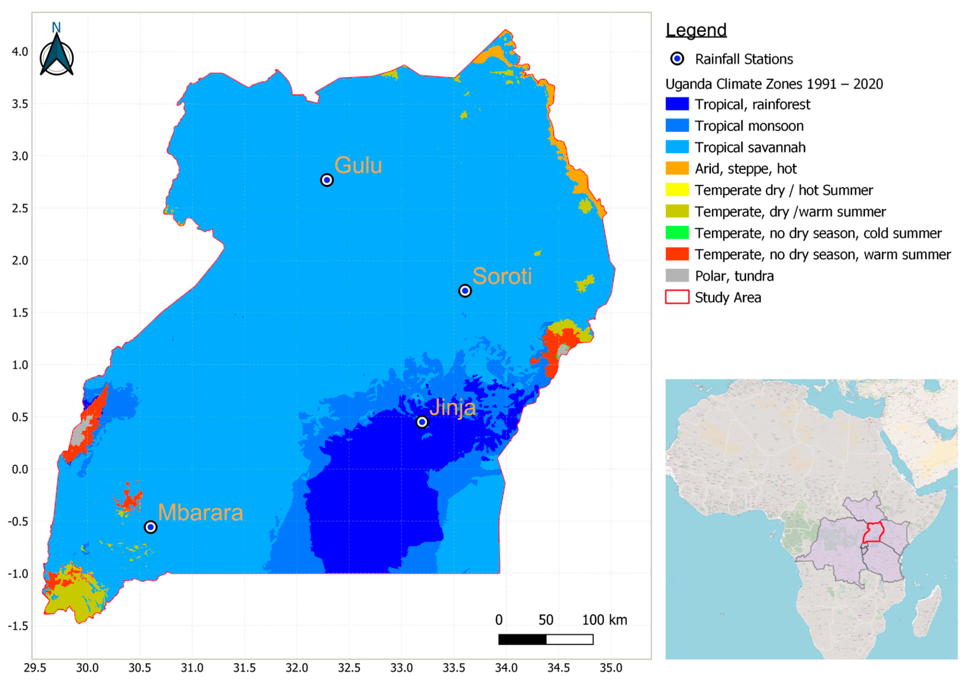
Figure 1. Map of Uganda showing four rainfall stations across three climatic zones.
Sustainability 16 06081 g001
Figure 2. Flowchart of methodology.
Sustainability 16 06081 g002
Figure 3. Flow chart of rainfall data quality control process.
Sustainability 16 06081 g003
Figure 4. Trend analysis methodological flow chart.
Sustainability 16 06081 g004
Figure 5. Gaps in observed rainfall data at the Jinja, Gulu, Mbarara, and Soroti rainfall stations.
Sustainability 16 06081 g005
Figure 6. Gaps in satellite-based rainfall data at the Jinja, Gulu, Mbarara, and Soroti rainfall stations: (a) Gaps in NOAA satellite rainfall data product and (b) gaps in PERSIANN satellite rainfall product.
Sustainability 16 06081 g006
Figure 7. Outlier detection at the Gulu rainfall station: (a) From time series plot and (b) from IQR boxplot.
Sustainability 16 06081 g007
Figure 8. Trends in seasonal rainfall: (a) MAM season and (b) SON season.
Sustainability 16 06081 g008
Figure 9. Trends in AMS rainfall data.
Sustainability 16 06081 g009
Figure 15. PDF and CDF of distributions of the observed AMS and RSR dataset at the Soroti station.
Sustainability 16 06081 g015
Figure 16. PDF and CDF of distributions of the observed AMS and RSR dataset at the Mbarara station.
Sustainability 16 06081 g016
Figure 17. PDF and CDF of distributions of the observed AMS and RSR dataset at the Gulu station.
Sustainability 16 06081 g017
Table 3. Trend analysis test results for seasonal rainfall at the Mbarara station.
RainfallSeasonTaup-ValueSlope (mm/Year)R2 ValueTrendStatistical Significancy
ObservedMAM0.050.721.320.02IncreasingNot significant
SON−0.010.95−0.110DecreasingNot significant
CHIRPSMAM0.150.241.780.08IncreasingNot significant
SON0.030.80.060IncreasingNot significant
ERA5_AGMAM−0.080.57−0.50.01DecreasingNot significant
SON0.090.480.220IncreasingNot significant
MERRA2MAM0.406.230.28IncreasingSignificant
SON0.310.024.950.26IncreasingSignificant
NOAA_CPCMAM0.30.024.970.12IncreasingSignificant
SON0.260.0440.17IncreasingSignificant
PERSIANNMAM−0.010.940.060IncreasingNot significant
SON−0.20.13−1.620.07DecreasingNot significant
ERA5MAM−0.10.46−0.790.01DecreasingNot significant
SON0.140.31.250.02IncreasingNot significant
GPCCMAM−0.0011−0.380DecreasingNot significant
SON01−0.150DecreasingNot significant
Table 4. Trend analysis test results for seasonal rainfall at the Soroti station.
RainfallSeasonTaup-ValueSlope (mm/Year)R2 ValueTrendStatistical Significancy
ObservedMAM0.010.97−2.170.03DecreasingNot significant
SON−0.020.891.280.01IncreasingNot significant
CHIRPSMAM0.090.480.990.01IncreasingNot significant
SON0.130.323.630.11IncreasingNot significant
ERA5_AGMAM−0.10.44−1.410.03DecreasingNot significant
SON010.380IncreasingNot significant
MERRA2MAM0.130.322.370.04IncreasingNot significant
SON0.170.194.730.15IncreasingNot significant
NOAA_CPCMAM0.030.860.750IncreasingNot significant
SON0.070.620.920.01IncreasingNot significant
PERSIANNMAM−0.090.48−1.130.02DecreasingNot significant
SON−0.060.67−0.290DecreasingNot significant
ERA5MAM−0.120.36−1.80.05DecreasingNot significant
SON0.050.71.140.01IncreasingNot significant
GPCCMAM0.110.41.920.02IncreasingNot significant
SON0.090.51.660.02IncreasingNot significant
Table 5. Trend analysis test results for seasonal rainfall at the Jinja station.
RainfallSeasonTaup-ValueSlope (mm/Year)R2 ValueTrendStatistical Significancy
ObservedMAM−0.040.75−2.170.03DecreasingNot Significant
SON0.150.263.340.05IncreasingNot Significant
CHIRPSMAM0.280.034.410.22IncreasingSignificant
SON0.240.067.990.25IncreasingNot Significant
ERA5_AGMAM−0.090.48−2.000.03DecreasingNot Significant
SON−0.170.19−2.120.05DecreasingNot Significant
MERRA2MAM−0.260.04−9.550.22DecreasingSignificant
SON−0.030.83−0.750.00DecreasingNot Significant
NOAA_CPCMAM−0.130.34−3.960.07DecreasingNot Significant
SON0.090.482.400.05IncreasingNot Significant
PERSIANNMAM−0.030.800.310.00DecreasingNot Significant
SON0.080.552.000.03IncreasingNot Significant
ERA5MAM−0.080.57−1.150.01DecreasingNot Significant
SON−0.190.14−1.660.03DecreasingNot Significant
GPCCMAM−0.020.92−0.070.00DecreasingNot Significant
SON0.070.622.170.02IncreasingNot Significant
Table 6. Trend analysis test results for AMS rainfall at the Jinja station.
RainfallTaup-ValueSlope (mm/Year)R2 ValueTrendStatistical Significancy
Observed−0.090.50−0.360.03DecreasingNot Significant
CHIRPS0.090.500.170.03IncreasingNot Significant
ERA5_AG−0.130.32−0.340.02DecreasingNot Significant
MERRA20.040.780.180.01IncreasingNot Significant
NOAA_CPC−0.200.13−1.320.21DecreasingNot Significant
PERSIANN0.020.89−0.010.00IncreasingNot Significant
ERA50.190.150.350.06IncreasingNot Significant
GPCC−0.010.94−0.340.03DecreasingNot Significant
Table 7. Trend analysis test results for AMS rainfall at the Soroti station.
RainfallTaup-ValueSlope (mm/Year)R2 ValueTrendStatistical Significancy
Observed−0.050.68−0.340.03DecreasingNot Significant
CHIRPS−0.220.09−0.330.11DecreasingNot Significant
ERA5_AG0.130.340.370.04IncreasingNot Significant
MERRA20.020.920.300.04IncreasingNot Significant
NOAA_CPC0.210.110.320.02IncreasingNot Significant
PERSIANN−0.100.460.080.01IncreasingNot Significant
ERA50.160.210.370.06IncreasingNot Significant
GPCC−0.140.30−0.620.09DecreasingNot Significant
Table 8. Trend analysis test results for AMS rainfall at the Mbarara station.
RainfallTaup-ValueSlope (mm/year)R2 ValueTrendStatistical Significancy
Observed0.010.930.230.01IncreasingNot Significant
CHIRPS0.040.780.090.01IncreasingNot Significant
ERA5_AG0.540.000.650.37IncreasingSignificant
MERRA20.370.001.030.25IncreasingSignificant
NOAA_CPC−0.150.24−0.500.05DecreasingNot Significant
PERSIANN0.080.550.040.00IncreasingNot Significant
ERA50.430.000.480.21IncreasingNot Significant
GPCC0.040.780.060.00IncreasingNot Significant
Table 9. Trend analysis test results for AMS rainfall at the Gulu station.
RainfallTaup-ValueSlope (mm/Year)R2 ValueTrendStatistical Significancy
Observed0.160.210.600.08IncreasingNot Significant
CHIRPS−0.110.42−0.170.05DecreasingNot Significant
ERA5_AG0.130.320.080.01IncreasingNot Significant
MERRA20.250.051.300.13IncreasingNot Significant
NOAA_CPC0.220.091.060.14IncreasingNot Significant
PERSIANN−0.220.09−0.030.00DecreasingNot Significant
ERA50.030.830.010.00IncreasingNot Significant
GPCC0.050.700.390.02IncreasingNot Significant
Disclaimer/Publisher’s Note: The statements, opinions and data contained in all publications are solely those of the individual author(s) and contributor(s) and not of MDPI and/or the editor(s). MDPI and/or the editor(s) disclaim responsibility for any injury to people or property resulting from any ideas, methods, instructions or products referred to in the content.