Abstract
The advent of high-resolution minute-level traffic flow data from video surveillance on roads has opened up new opportunities for enhancing the estimation of traffic noise levels. In this study, we propose an innovative method that utilizes time series traffic flow data (TSTFD) to estimate traffic noise levels using a deep learning Convolutional Neural Network (CNN). Unlike traditional traffic flow data, TSTFD offer a unique structure and composition suitable for multidimensional data analysis. Our method was evaluated in a pilot study conducted in Foshan City, China, utilizing traffic flow information obtained from roadside video surveillance systems. Our results indicated that the CNN-based model surpassed traditional data-driven statistical models in estimating traffic noise levels, achieving a reduction in mean squared error (MSE) by 10.16%, mean absolute error (MAE) by 4.48%, and an improvement in the coefficient of determination (R²) by 1.73%. The model demonstrated robust generalization capabilities throughout the test period, exhibiting mean errors ranging from 0.790 to 1.007 dBA. However, the model’s applicability is constrained by the acoustic propagation environment, demonstrating effectiveness on roads with similar surroundings while showing limited applicability to those with different surroundings. Overall, this method is cost-effective and offers enhanced accuracy for the estimation of traffic noise level.
1. Introduction
Traffic noise pollution has surged significantly with the exponential growth in vehicle traffic, posing a major environmental challenge in densely populated urban areas globally [1,2,3]. Prolonged exposure to a noise-polluted environment can precipitate a range of psychological and physiological issues, including hearing impairment, diabetes mellitus, annoyance, hypertension, and cardiovascular disease [4,5,6,7,8]. The accurate and quantitative characterization of traffic noise is essential for assessing its suitability for human habitation [9,10]. Generally, traffic noise is quantified either through physical monitoring or mathematical modeling [11]. While physical monitoring is resource-intensive and costly, mathematical modeling offers a more economical alternative, utilizing traffic flow data often gathered from existing roadside video surveillance systems.
Since the 1950s, various mathematical models have been developed to estimate traffic noise levels [11]. These models fall into two primary categories: acoustic-based numerical models and data-driven statistical models. Acoustic-based numerical models, such as the Federal Highway Administration (FHWA) model in the U.S., the Calculation of Road Traffic Noise (CRTN) model in the UK, the European Common Noise Assessment Methods in Europe model (CNOSSOS-EU), and the Chinese criterion model of the Technical Guidelines for Noise Impact Assessment (HJ-21) in China [12,13,14,15,16], focus on the propagation, reflection, and absorption of sound but require specialized knowledge and are based on strict assumptions [17]. Conversely, data-driven statistical models like Artificial Neural Network (ANN) models, Support Vector Machine (SVM) models, and Multiple Linear Regression (MLR) models leverage diverse data types and advanced statistical techniques to model complex relationships among variables, enhancing the precision of traffic noise levels estimations [18,19,20,21,22,23,24,25,26]. A comparison of the different features of the models is shown in Table 1.

Table 1.
Comparison of developed models.
Historically, aggregated traffic flow data (ATFD) have been used, which are averaged and aggregated over the estimation period due to resource constraints [1,27,28]. However, this approach may not adequately account for traffic flow fluctuation variations. To tackle this issue, utilizing time series traffic flow data (TSTFD) becomes crucial, as they offer high-resolution minute-level traffic data to capture traffic flow fluctuations effectively, thereby enhancing the accuracy of traffic noise level estimations. Time series data are becoming more accessible due to the proliferation of video surveillance systems along roads [29]. While TSTFD have been extensively used in traffic flow prediction [30,31], their application to the estimation of traffic noise levels is rarely reported publicly. Compared to the aforementioned mathematical models, the Convolutional Neural Network (CNN), known for its proficiency in extracting features from multidimensional structured data, presents a promising method for utilizing TSTFD in noise estimation [32,33]. Although the CNN is widely used in various domains like image classification, target localization, and facial recognition [34,35,36], its potential in traffic noise modeling is yet to be fully explored.
In this study, we propose a novel method to estimate traffic noise levels by utilizing CNN based on TSTFD. To comprehensively evaluate the performance of this method, we compared it with widely used traditional models like the ANN, MLR, and HJ-21. Subsequently, a pilot study was conducted in Foshan City, China, renowned for its substantial traffic noise pollution, to validate the method’s performance. The results from our study indicate that the CNN model significantly enhances the accuracy of traffic noise level estimations, demonstrating the effectiveness of this innovative method.
2. Material and Method
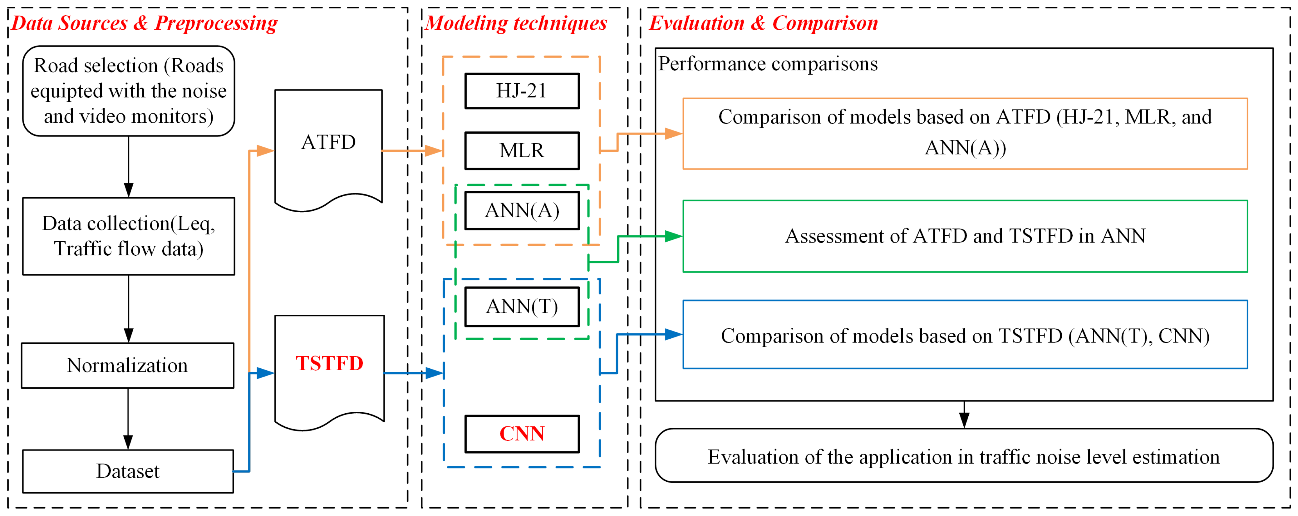
The study methodology comprises three stages, as illustrated in Figure 1. Initially, five roads equipped with noise monitors and video surveillance systems were selected to collect equivalent continuous sound pressure levels (Leq) and traffic flow data. The traffic flow data were processed using two different types of data: ATFD and TSTFD. Subsequently, various modeling techniques, including the CNN, ANN, MLR, and HJ-21, were utilized to develop a total of five estimation models. The ANN stands out as a prevalent deep learning model known for its high performance at present [26]. Meanwhile, MLR has been extensively utilized in early research for traffic noise level estimations [23]. Additionally, HJ-21, developed by the Ministry of Ecology and Environment of China, serves as a traffic noise estimation model tailored for urban roads in China [16]. Finally, comparative analyses were conducted to evaluate the performance improvement in traffic noise level estimation achieved by utilizing the CNN model based on TSTFD. Further details are provided below.
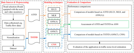
Figure 1.
Technical flow diagram for enhanced estimation of traffic noise levels through a Convolutional Neural Network. Note: HJ-21, MLR, and ANN(A) models are developed using aggregated traffic flow data (ATFD); ANN(T) and CNN models are developed using time series traffic flow data (TSTFD).
2.1. Data Sources and Preprocessing
In 2022, 43.4% of monitored roads (out of the 300.73 km) in Foshan, China had an excessive ambient noise problem, exceeding 70 dBA. Following the road selection criteria listed in Supporting Information (SI) (Section S1), the selected five roads in Foshan were LZ Road (Road_1), FC Road (Road_2), BC Road (Road_3), GN Road (Road_4), and CC Road (Road_5) (Figures S1 and S2). These roads were divided into two groups, Group A and Group B, based on the similarity of their surroundings, to develop the models and evaluate their performance (Section S2). The fundamental features of the roads are listed in (Table S1). Data collection was conducted in July 2023 on the aforementioned roads (Section S3). The traffic flow data consisted of six variables: light, medium, and heavy vehicle flows, as well as light, medium, and heavy vehicle speeds. Due to the varying dimensions of these variables, normalization was applied to standardize the input variables (Section S5), thereby mitigating the potential masking of low-value variables by those with higher values [37,38]. Subsequently, each successive 10 min segment of the traffic flow data was processed using two different data types: ATFD and TSTFD (Section S6), to assess and compare the performance of estimating traffic noise levels. ATFD were calculated by aggregating and averaging the data over each 10 min interval, while TSTFD consisted of these data arranged in chronological order. Finally, the datasets for 10 min intervals are listed in (Table S4).
2.2. Convolutional Neural Network
The architecture of the CNN is specifically designed to handle multidimensional structured data, leveraging the highly effective convolutional kernel for feature extraction [32]. TSTFD can be considered as two-dimensional data continuously sampled along the time axis, encompassing variable and temporal dimensions. Therefore, the CNN is expected to extract features of traffic flow fluctuations from such time series data. The process of modeling the CNN is as follows.
Firstly, the activation function in multilayer neural networks plays a crucial role in enabling nonlinear mappings between inputs and outputs, which is essential in modeling complex relationships, such as those between traffic flow variables and noise levels. The Sigmoid function had been widely applied in traffic noise estimation tasks [25,37] and was selected as the activation function in this study. The formulation can be expressed as Equation (1).
where x is the input value.
Secondly, the Adaptive Moment Estimation (Adam) optimization algorithm was utilized to train deep learning models. Adam combines the momentum technique with an adaptive learning rate to enhance the efficiency of the gradient descent algorithm [39]. The formulations can be expressed as Equations (2)–(6).
where is the momentum at the current moment, is the gradient at the current moment, is the momentum decay coefficient, and is the uncentered variance at the current moment. is the uncentered variance decay coefficient, is the bias-corrected mt, is the bias-corrected , is the model parameter at the current moment, and is a small constant added for numerical stability.
Next, the loss function quantifies the error between the outputs and the actual values. This error is directly measured using the mean squared error (MSE), providing an intuitive assessment of a regression model’s estimated accuracy [40]. The MSE was selected as the loss function due to the regression problem of estimating traffic noise levels. The formulation can be expressed as Equation (7).
where m is the total number of data samples, yi is the actual value, is the estimated output, and is the average value of the actual value.
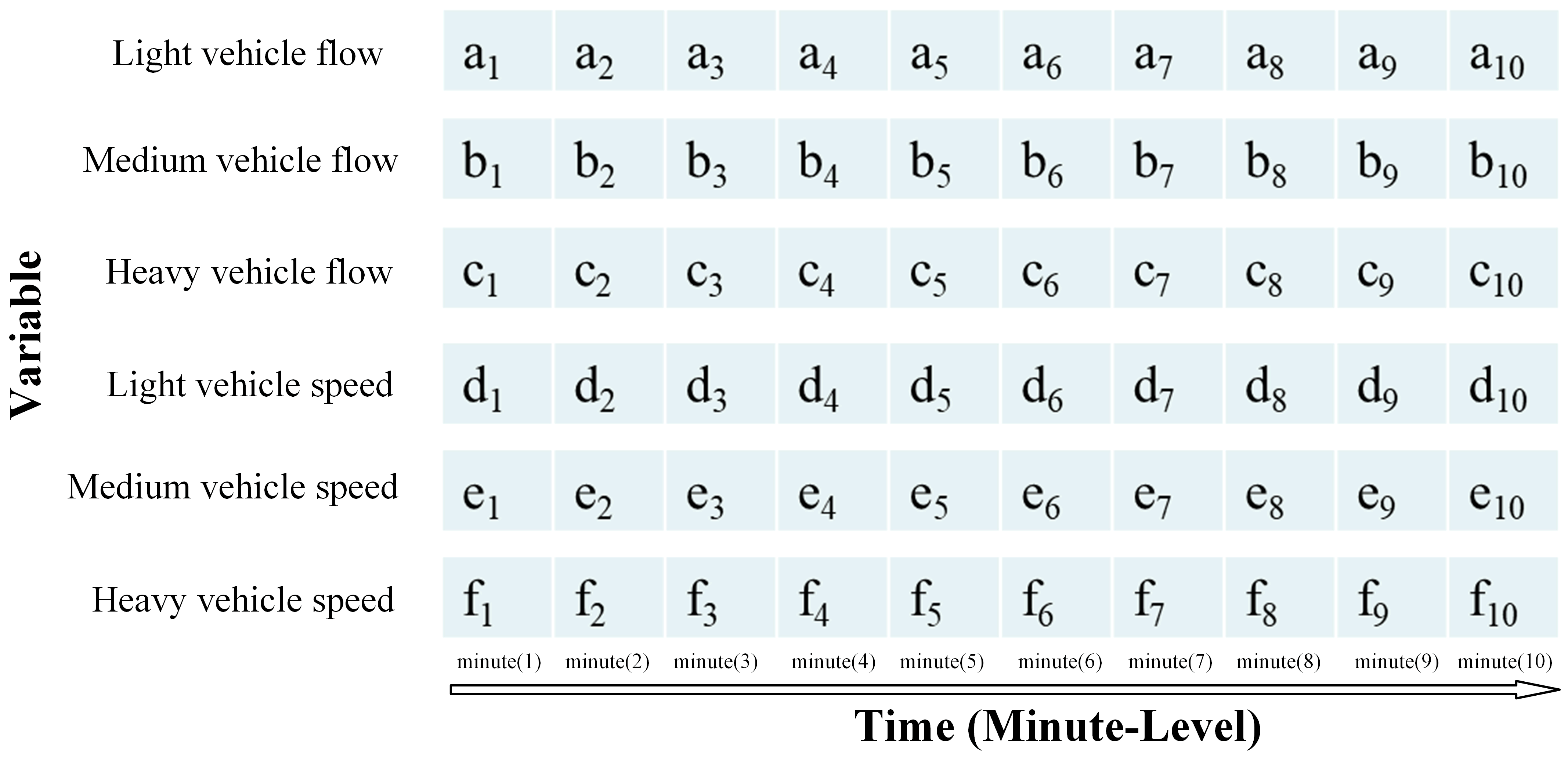
When designing the CNN architecture, two crucial considerations arise: (1) determining the relevant hyperparameters for the convolutional layers and pooling layers, including the size of the convolutional kernel, the size of the pooling window, and the pooling method selection; and (2) deciding the depth of the architecture [41]. The time series data for each variable were represented as a vector of length 10, which combined to form a two-dimensional matrix with a size of 6 × 10, corresponding to the six variables it represented Figure 2. Considering the input size of 6 × 10, a 1 × 3 one-dimensional convolutional kernel was chosen, and the pooling window size was set to 1 × 2. In the case of the same receptive field, smaller convolutional kernels and pooling windows help to build a deeper network architecture, improving the ability of the model to extract features [42]. The max pooling method was utilized to emphasize the prominent features within the input. The CNN model extracted traffic flow features through the following process: (1) The two-dimensional traffic flow matrix underwent processing in a convolutional block, comprising convolutional layers and a max pooling layer. The convolution layer organized units into feature maps, with the max pooling layer consolidating semantic features into a unified map [43]. (2) The matrix traversed all convolution blocks until reaching the fully connected layer, which included a flattened layer and multiple dense layers. The flattened layer reduced the feature map to a single column for input into the fully connected layer, while the dense layers established connections within the neural network. (3) Consequently, the layer preceding the fully connected layer extracted crucial “traffic flow features” from the matrix.
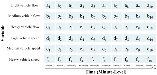
Figure 2.
The data structure of time series traffic flow data.
In this study, the depth of the CNN architecture proposed is derived from LeNet-5, a commercially available CNN structure known for its excellent performance [44,45]. To determine the optimal depth of the network architecture, experiments with three different depths were conducted using a trial-and-error method (Figure S4). The experimental results showed that increasing the model depth did not improve the performance (Table S5). The model architecture with two convolutional layers was selected as the final network architecture (Figure S4a). Additional hyperparameter configurations are elaborated in Section S7.
2.3. Model Training and Evaluation
Three sets of controlled experiments were conducted to thoroughly evaluate the performance improvement in estimating traffic noise levels by utilizing a CNN model based on TSTFD. Firstly, the performances of commonly used models, such as the ANN, MLR, and HJ-21 (Section S8), were evaluated. Secondly, using the ANN model, we assessed the performance of TSTFD and ATFD in estimating traffic noise levels under various traffic flow fluctuations. Finally, the performances of the ANN and CNN based on TSTFD were compared to evaluate their improvement for this task. As a result, a total of five estimation models were developed by using four modeling techniques, either based on ATFD or TSTFD (Figure S6). Estimation models were developed separately for each modeled road to mitigate the influence of other factors, such as road characteristics and the surrounding environment. The TensorFlow platform was utilized to construct and train the estimation models. The configuration of the experimental environment is listed in Table S6.
The models presented above utilized a 10-fold cross-validation method (Section S9) to select the parameter with the best performance. To investigate the interpretability of the model, a feature sensitivity analysis was conducted to identify the primary factor that had a significant impact on traffic noise (Section S10). Subsequently, further analysis of the fluctuations in this factor was conducted to uncover the underlying reasons for the observed performance improvement. Furthermore, the estimation models were applied to estimate traffic noise levels on different roads. The performance metrics, including the coefficient of determination (R2), mean squared error (MSE), and mean absolute error (MAE), were utilized to provide a measure of estimation accuracy (Section S11).
3. Result and Discussion
3.1. Improvement of Estimation Accuracy
The evaluation results for the modeled roads, including Road_1, Road_2, and Road_3, are presented in (Figure S7) using a 10-fold cross-validation method. Among the traditional models based on ATFD, the average performance was measured using the MSE values for the ANN(A), MLR, and HJ-21 models, which were 1.543, 2.502, and 4.486, respectively. The results indicated that the ANN(A) model exhibited the best performance, followed by the MLR model, and finally the HJ-21 model. The superior performance of the ANN(A) model can be attributed to its ability to extract complex nonlinear relationships within traffic noise systems as supported by previous studies comparing the ANN and MLR models for traffic noise level estimation [19,24]. On the other hand, the poorest performance of the HJ-21 model can be attributed to the need for domain-specific expertise in calibrating acoustic-based numerical models, as well as the stricter underlying assumptions associated with such models [17].
In addition to ATFD, this study proposed to estimate traffic noise levels by using TSTFD. Considering that TSTFD offer unique information not found in ATFD, it is crucial to quantify the fluctuations in traffic flow to better evaluate the performance of utilizing TSTFD. Firstly, the relative importance of traffic flow features was quantified by a feature removal sensitivity analysis method based on the ANN(A), ANN(T), and CNN models, as illustrated in Figure 3. The results indicated that light vehicle flow (LF) was the most important feature for Road_1 and Road_2, while medium vehicle flow (MF) held the most importance for Road_3. This difference in importance may arise from the traffic composition of Road_3, where the higher proportion of MF (14.92%) resulted in a greater contribution to the traffic noise level compared to Road_1 and Road_2, due to the positive correlation between traffic flow and noise levels Table 2. Conversely, the lower proportion of LF (71.53%) in Road_3 led to a reduced contribution compared to Road_1 and Road_2 Table 2. As a result, the contribution of MF to the traffic noise levels on Road_3 might exceed that of LF, making MF the most important feature. Secondly, the fluctuations in these traffic flow features were quantified by the average value of variances (AVOV) (Section S12). The AVOV values for the most important feature, LF, on Road_1 and Road_2, were 125.333 and 61.13, respectively. The MF on Road_3 had a much lower AVOV value of only 5.195 (Table 2). According to the AVOV values, the ranking of the degree of fluctuation in the most important feature for the modeled road was as follows: Road_1, Road_2, and Road_3, from largest to smallest.
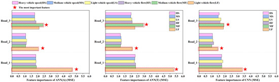
Figure 3.
The relative importance of traffic flow features in estimating traffic noise levels. Note: the red box represents the most important feature.
Table 2.
The proportion and AVOV of each vehicle type on the modeled roads.
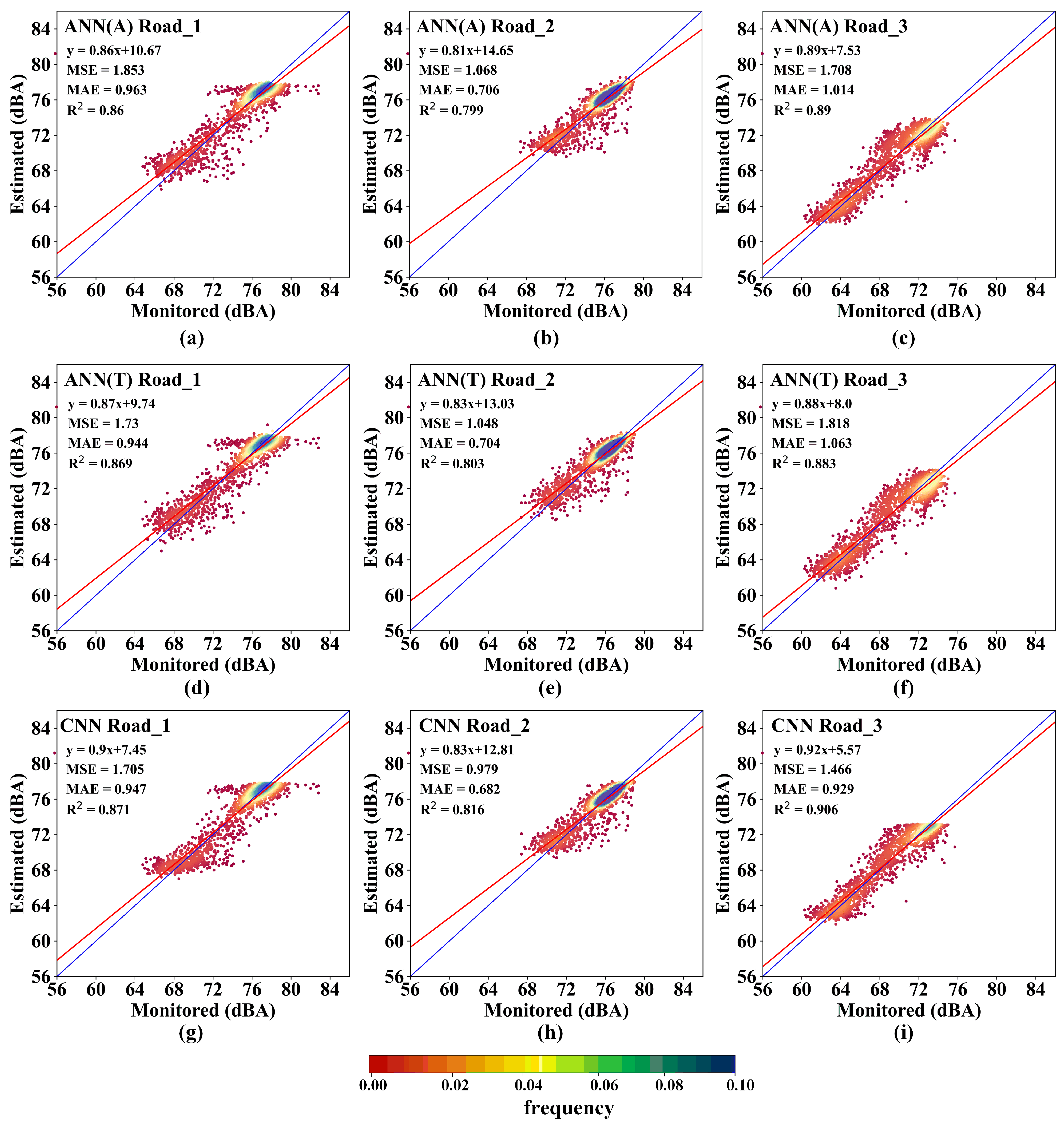
Based on the aforementioned results regarding traffic flow fluctuations, the performance of the models based on TSTFD and ATFD was evaluated by comparing the ANN(A) and ANN(T) models. The scatter density plots for the ANN(A) model and ANN(T) model are shown in Figure 4a–f. Figure 4 clearly illustrates that the data points are concentrated in areas with relatively high noise levels, suggesting that a significant proportion of the monitored data represent high-noise-level samples. Furthermore, the data points are clustered on both sides of the reference line (blue line), indicating a robust model fit. Compared to the ANN(A) model, the ANN(T) model exhibited improved performance in both Road_1 and Road_2. Particularly, the most significant improvement was observed in Road_1, where the MSE decreased by 6.66%, the MAE decreased by1.97%, and the R2 increased by 1.05%. In contrast, the performance of the ANN(T) model deteriorated in Road_3, resulting in an increase of 6.43% in MSE, an increase of 4.83% in MAE, and a decrease of 1.05% in R2. This trend aligned with the degree of fluctuation observed among the most important features of these roads. The utilization of TSTFD in the model development improved the accuracy of the traffic noise level estimations for Road_1 and Road_2, which experienced relatively larger traffic flow fluctuations (with AVOV values of 125.33 and 61.13, respectively). However, relying on TSTFD posed a disadvantage for the ANN model when the traffic flow fluctuation was relatively small, as in the case of Road_3. Road_3 exhibited the lowest fluctuation (with an AVOV value of 5.195) among the modeled roads, leading to more complex and subtle features of traffic flow fluctuation. The traditional ANN model demonstrated relative weakness in handling such complex and subtle feature extraction, necessitating a more powerful model. In contrast, the aggregated traffic flow depicted in ATFD may be more representative and better suited for the ANN model. To address this weakness, the CNN model was proposed to estimate traffic noise levels based on TSTFD, leveraging the advantages of feature extraction from multidimensional structured data.
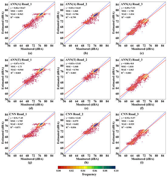
Figure 4.
Scattered density plots of the performance evaluation results. (a–c) ANN(A) model; (d–f) ANN(T) model; (g–i) CNN model. Note: the blue line represents the reference line, while the red line represents the fitted line.
The performance of the CNN model based on TSTFD for estimating traffic noise levels was evaluated by comparing them with the ANN model. The scatter density plots for the ANN(T) and CNN models are shown in Figure 4d–i. The CNN model consistently outperformed the ANN(T) model in estimating traffic noise levels for the modeled roads, with mean errors of 0.947 dBA, 0.682 dBA, and 0.929 dBA, respectively. The most significant improvement was observed in Road_3, where the MSE decreased by 19.33%, the MAE decreased by 12.61%, and the R2 increased by 2.60%. This was followed by Road_2 and Road_1. Notably, the magnitude of performance improvement correlated with the degree of the most important feature fluctuation, indicating that a smaller fluctuation resulted in a greater improvement. This improvement can be primarily attributed to the superior capability of the CNN model in extracting features from time series data compared to the ANN model [46]. This was elucidated as follows: (1) Utilizing a parameter-sharing mechanism, the CNN model facilitated weight sharing across various positions, thereby diminishing the number of model parameters [47]. (2) By leveraging the local receptive field of the convolutional layer, the CNN model adeptly extracted spatial features within the data [42]. (3) Through a series of multilayer convolution and pooling operations, the CNN model progressively extracted features of diverse data levels [48]. This advantage allowed the CNN model to handle smaller fluctuations with more complex and subtle features. Finally, the CNN model also outperformed the traditional model, such as the ANN(A) model, with an average performance decrease of 10.16% for MSE, 4.48% for MAE, and an increase of 1.73% for R2 across the modeled roads. Consequently, this study demonstrated the effectiveness of the novel method, a CNN model based on TSTFD, in improving the accuracy of traffic noise level estimation.
3.2. Evaluation of the Application in Traffic Noise Level Estimation
To evaluate the generalization performance of the CNN model based on TSTFD in practical applications, the model was applied to a new dataset that was collected for one day (15 July 2023) on the three modeled roads. The monitoring results indicate a positive correlation between traffic noise levels and traffic flow features, particularly the most important feature, with an R2 of 0.812, 0.714, and 0.827, respectively (Figure S8). In contrast, vehicle speed exhibited a weak correlation with traffic levels (Figure S8). These findings aligned with the results obtained from the feature sensitivity analysis discussed in the previous section. Throughout the nighttime, all monitored values exceeded the night noise level limit of 55 dBA, leading to a 0% night compliance rate. The traffic flow was relatively low or even negligible during this period, indicating that the background noise level on these roads might have already exceeded the night noise level limit. On the other hand, the daytime compliance rates for the modeled roads were 0%, 0%, and 17%, respectively. The low compliance rate was primarily attributed to the noise generated by vehicles due to the high traffic flow during the daytime.
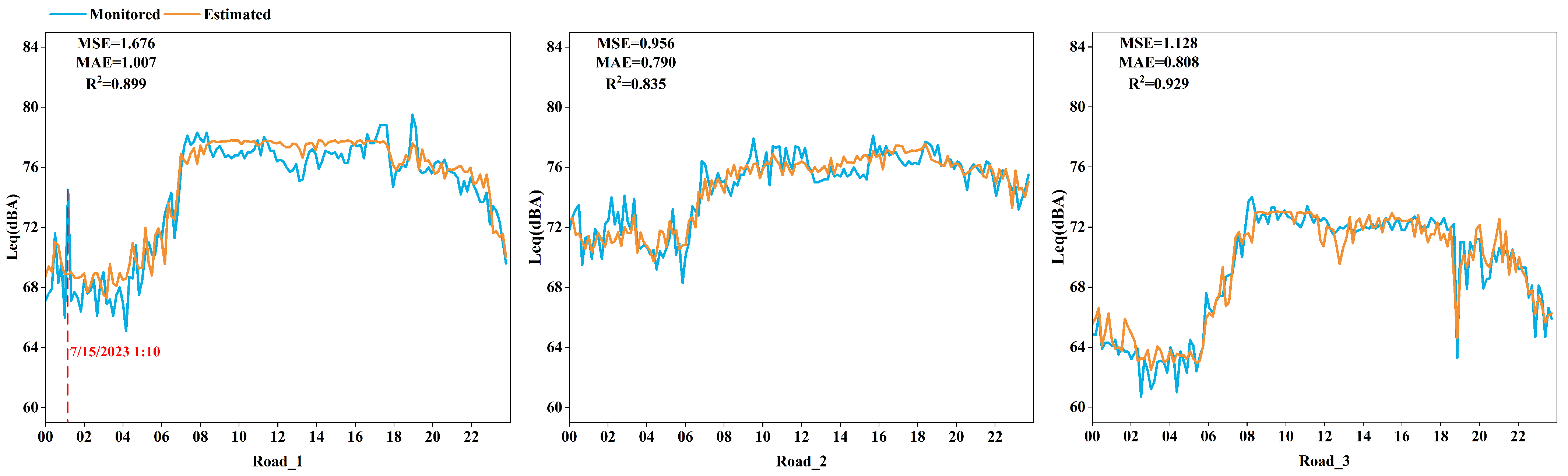
During the practical application, each fold model was utilized to assess the test data, resulting in 10 estimated results (comprising 10 fold models in each model). The average noise level from these 10 estimated results was considered as the model’s estimated results. The computational efficiency of the CNN, ANN(T), and ANN(A) models was assessed using 100 test samples. The results showed that the intricate structure and computational steps of the CNN led to a computation time almost double that of the ANN(T) and ANN(A) models (Table 3). The estimation results presented in Figure 5 show a significant overlap between the monitored and estimated values, with the MSE ranging from 0.956 to 1.676 and the R2 ranging from 0.835 to 0.929. These findings indicate the model’s ability to generalize well to unseen data during the training period. Compared to the ANN(A) and ANN(T) models, the CNN model demonstrated higher accuracy, with an MAE of 1.007, 0.790, and 0.808, respectively (Table S8). Among the results, the largest error occurred at 1:10 on 15 July 2023, on Road_1, with an estimation error of 5.3 dBA. The traffic flow information for the half hour before and after this time indicated that the traffic flow was relatively smooth (Table S9). Therefore, the error can be attributed to sudden noise events that are difficult for the model to capture.
Table 3.
The computation time of models tested for 100 samples.
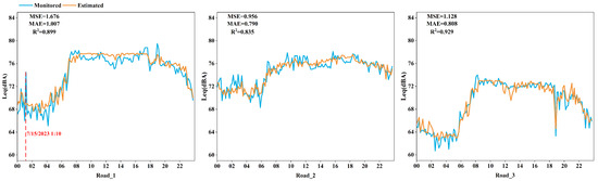
Figure 5.
Estimation results of the CNN model on the modeled roads (15 July 2023).
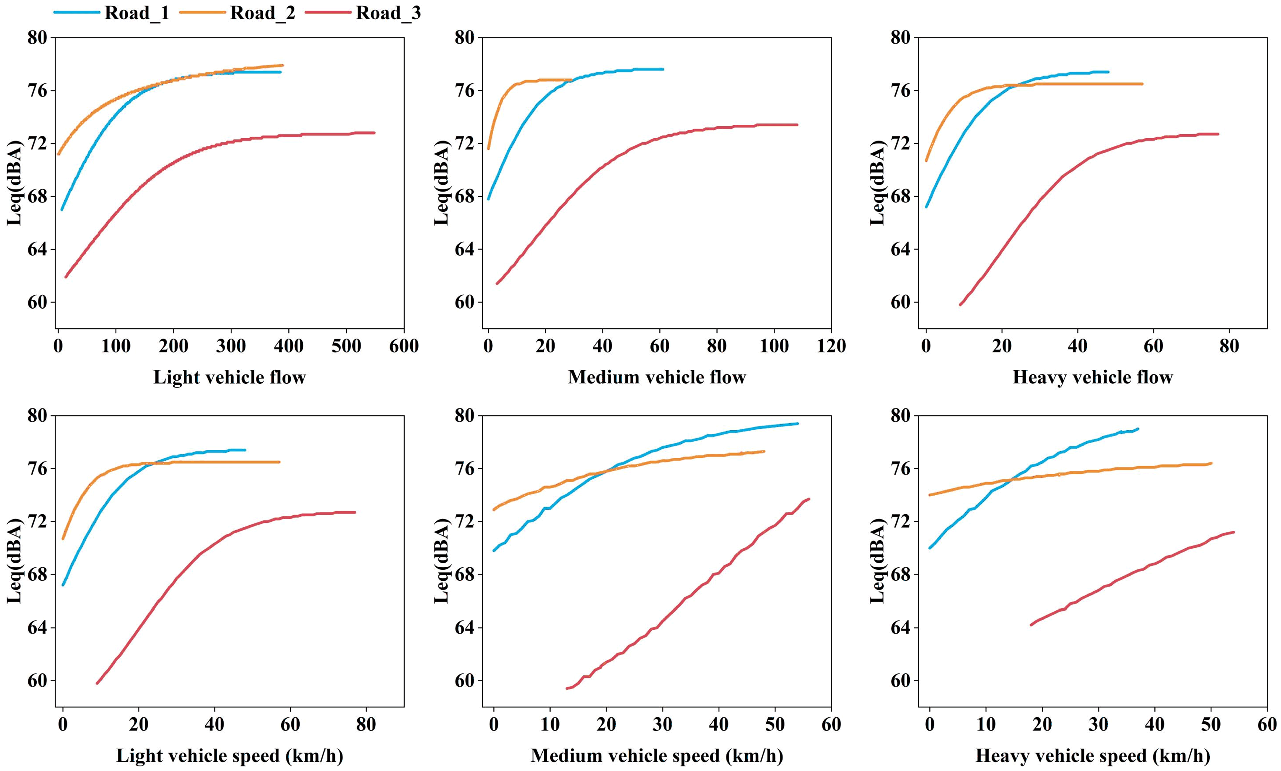
To further evaluate the generalization performance, we used the models to estimate traffic noise levels on different roads. Initially, this was conducted among the three modeled roads. For instance, the Road_1 model was applied to estimate traffic noise levels on Road_2 (hereinafter referred to as 1–2), and so on. Among the modeled roads, Road_1 and Road_2, which had similar surroundings, were classified as Group A, while Road_3 belonged to Group B. For the modeled road and its corresponding target road within the same group, such as 1–2 and 2–1, the average performance of the CNN model resulted in MSE values of 5.424 and 5.143, respectively (Table S10). Conversely, when they belonged to different groups, such as 1–3, 3–1, 2–3, and 3–2, the MSE values were 57.564, 67.865, 56.361, and 103.012, respectively (Table S10). These results demonstrated a significant performance improvement when estimating noise levels within the same group of roads compared to across different groups. This improvement was also observed in the ANN(T) and ANN(A) models (Table S10). This can be primarily attributed to the oversight of factors such as road surface conditions, obstructing buildings along roadsides, road width, and other factors influencing noise propagation. While these factors may have minimal impact on the modeled road itself, they significantly vary between the modeled road and the target road. Consequently, the mapping relationships between traffic flow features and traffic noise levels differed between the modeled road and the target road. The mapping relationships were quantitatively characterized using a single feature analysis method, as depicted in Figure 6. The similar surroundings of Road_1 and Road_2 imply that their noise propagation surroundings are similar, resulting in a similar mapping relationship. Thus, the generalization performance of the model improved when both the modeled road and the target road had similar surroundings.
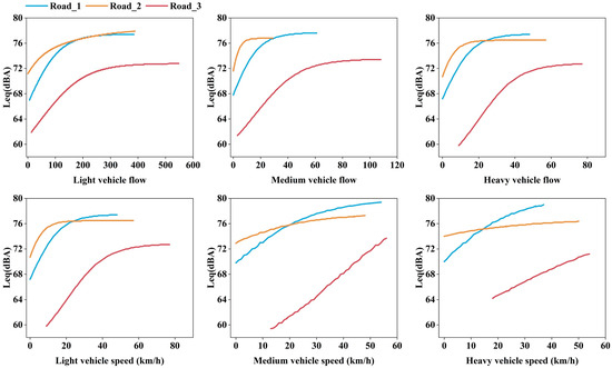
Figure 6.
The mapping relationships between traffic flow features and traffic noise levels.
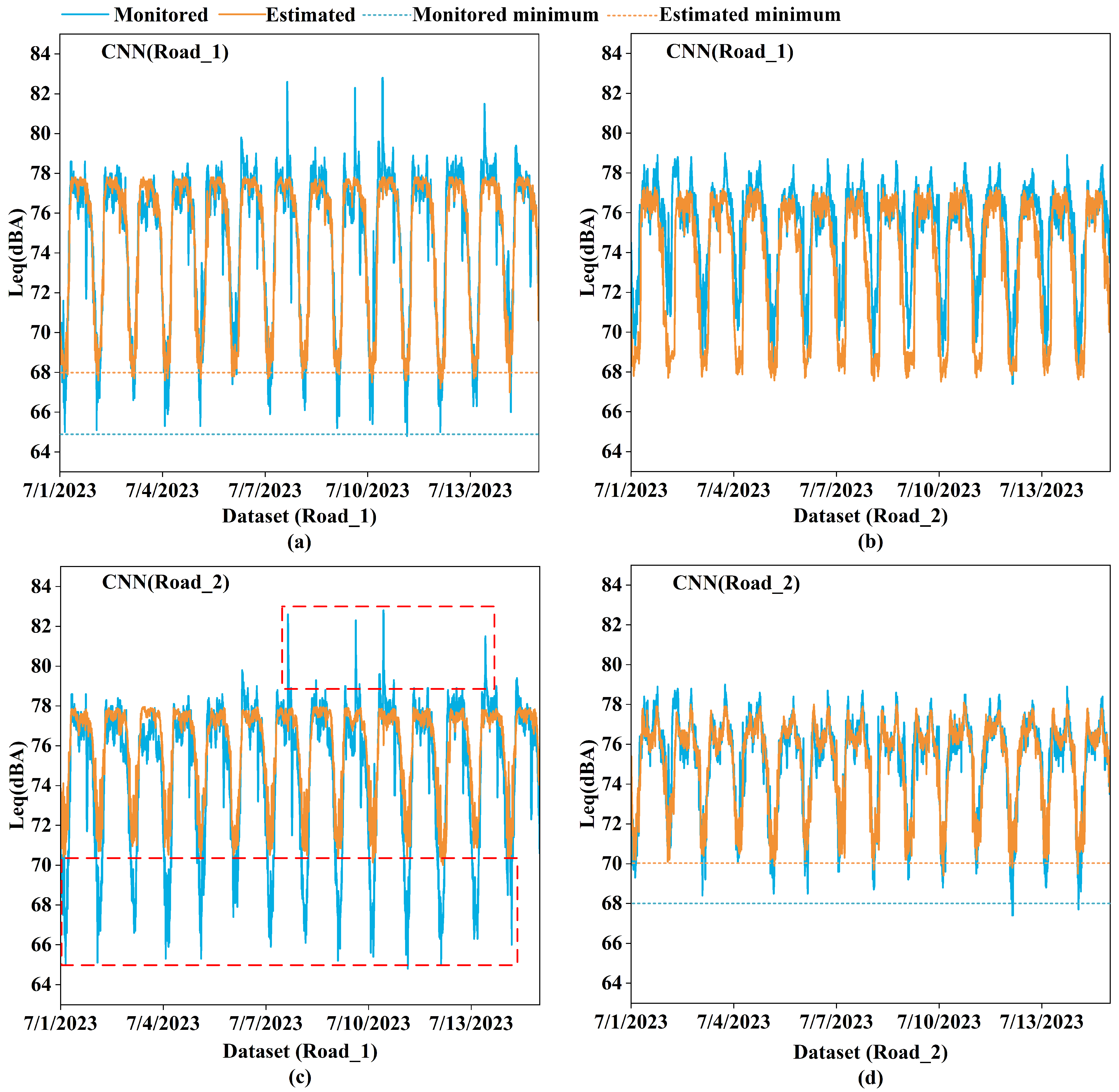
When evaluating the performance of similar roads, for the 1–2 performance, the MSE values of the CNN, ANN(T), and ANN(A) models were 5.124, 5.531, and 5.617, respectively (Table S10). Similarly, as for the 2–1 performance, the MSE values of the CNN, ANN(T), and ANN(A) models were 4.772, 5.010, and 5.756, respectively (Table S10). These results demonstrated that the CNN model outperformed both the ANN(T) model and the ANN(A) model. Comparing the ANN(A) model, the MSE values of the ANN(T) model decreased by 1.5% and 13.0%, respectively. This indicated that incorporating time series data proved advantageous in improving the generalization of the model. On the other hand, compared to the ANN(T) model, the MSE values of the CNN model decreased by 7.4% and 6.9%, respectively. The CNN model enhanced generality in tasks involving multidimensional structured data by reducing the number of parameters through mechanisms such as parameter sharing and weight sharing [49]. During cross-validation between Road_1 and Road_2, the estimation errors were mainly concentrated in the low-value range and the four peaks when using the Road_2 model to estimate traffic noise levels on Road_1, as depicted in the red box in Figure 7c. Low noise levels typically occurred at night when traffic flow was low. During these periods, Road_1 and Road_2 had monitored minimum values of 65 dBA and 68 dBA, respectively (Figure 7a,d).
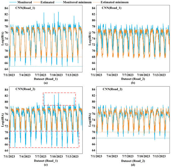
Figure 7.
Estimation results of the CNN model on Road_1 and Road_2. (a) shows the Road_1 model on Road_1; (b) shows the Road_1 model to estimate traffic noise levels on Road_2; (c) shows the Road_2 model to estimate traffic noise levels on Road_1; (d) shows the Road_2 model to estimate traffic noise levels on Road_2. Note: the red box indicates the primary concentration areas of estimation errors.
This difference arises from the distinct mapping relationships between traffic flow features and traffic noise levels for these two roads, with Road_1 exhibiting lower noise levels under low-traffic-flow conditions (Figure 6). In addition, the estimated minimum values were often higher than the monitored minimum values due to the insufficient sample data for extreme values, making it challenging to capture the features associated with these extreme values. There was a 5 dBA difference between the monitored minimum (65 dBA) value of Road_1 and the estimated minimum values (70 dBA) of the Road_2 model, resulting in larger estimation errors in the low-value range. As for the four estimation errors in peak noise levels, the traffic flow was relatively smooth during these periods (Tables S11 and S12). Therefore, these errors could be attributed to some sudden noise events occurring near the monitoring equipment along Road_1.
Additionally, we also applied the models to estimate traffic noise levels for Road_4 and Road_5, which served as outer verification cases. Road_4 was classified under Group A because of its similarity to the surroundings of Road_1 and Road_2, while Road_5 belonged to Group B. Regarding the CNN performance, the MSE values of the Road_1 and Road_2 models for estimating Road_4 were 2.460 and 1.808, respectively (Table 4). Similarly, for estimating Road_5, the MSE values were 40.684 and 56.688, respectively (Table 4). On the other hand, the Road_3 model had an MSE of 3.629 for estimating Road_5 and an MSE of 64.130 for estimating Road_4 (Table 4). These findings revealed that the CNN model of Road_1 and Road_2 exhibited higher accuracy in estimating traffic noise levels for Road_4 compared to Road_5. Similarly, the CNN model of Road_3 demonstrated higher accuracy in estimating the noise levels for Road_5 in comparison to Road_4. This result was also observed for the ANN(A) model and the ANN(T) model, further substantiating that the estimation models performed better in estimating noise levels when the modeled road and the target road had similar surroundings. Specifically, when the CNN model was applied to roads with similar surroundings, the average MSE of both Road_1 and Road_2 for Road_4 was 2.134, and the MSE of Road_3 for Road_5 was 3.629 (Table 4). These MSE values were lower than those in both the ANN(A) model and ANN(T) model, further demonstrating the superior generalizability of the CNN model in practical applications.
Table 4.
The generalization evaluation results of the model on Road_4 and Road_5 with the performance metric of MSE.
4. Conclusions
In this study, we introduced a novel method for estimating traffic noise levels by integrating TSTFD with a CNN model. The primary objective was to enhance the accuracy of traffic noise level estimations by effectively capturing the fluctuations in traffic flow. The application of this method in Foshan City, China, demonstrated its potential to outperform traditional methods significantly. Among the traditional methods, the ANN model based on ATFD showed commendable results, with performance metrics including an MSE of 1.543, an MAE of 0.894, and an R2 value of 0.849. The utilization of TSTFD improved the accuracy of traffic noise level estimation for roads with relatively larger traffic flow fluctuations. Furthermore, the application of the CNN model enhanced the feature extraction capability from TSTFD, resulting in a significant performance improvement compared to the traditional methods. Compared to the traditional method (the ANN model based on ATFD), there was a 10.16% decrease in MSE, a 4.48% decrease in MAE, and a 1.73% increase in R2. For the modeled roads, the MAE values were notably low, ranging between 0.682 dBA and 0.947 dBA. Therefore, this study substantiates that utilizing time series data can enhance the accuracy of traffic noise level estimations.
In practical applications, the proposed method demonstrated superior performance on the modeled road compared to traditional methods, with MAE values ranging from 0.790 to 1.007 dBA. While the method proved effective on roads with environmental conditions similar to those of the modeled roads, it faced limitations on roads with significantly different surroundings. This limitation suggests a need for model recalibration using localized data to ensure broader applicability. Moreover, additional variables will be integrated to broaden the model’s applicability across diverse road surroundings.
In conclusion, this study presents a cost-effective and technically advanced method for traffic noise level estimation. The use of existing roadside video surveillance systems for data collection underscores the practicality and scalability of this method, potentially setting a new standard in traffic noise assessment methodologies. Furthermore, it provides a robust framework to support environmental protection and traffic management authorities in making informed decisions to mitigate traffic noise pollution. Following the development of this method in the field of traffic noise estimation, it will be utilized in more challenging noise estimation scenarios, including social and industrial noise.
Supplementary Materials
The following supporting information can be downloaded at: https://www.mdpi.com/article/10.3390/su16146088/s1. References [37,50,51,52,53,54,55] are cited in the Supplementary Materials.
Author Contributions
Conceptualization, W.Y. (Wencheng Yu); methodology, W.Y. (Wencheng Yu); software, W.Y. (Wencheng Yu); validation, W.Y. (Wenwei Yang) and K.L.; formal analysis, J.-C.J., Y.Z. and J.P.; investigation, W.Y. (Wencheng Yu); resources, Y.Z.; data curation, W.Y. (Wencheng Yu); writing—original draft preparation, W.Y. (Wencheng Yu); writing—review and editing, J.-C.J., Y.Z., J.P., W.Y. (Wenwei Yang) and K.L.; visualization, W.Y. (Wencheng Yu); supervision, Y.Z.; project administration, Y.Z.; funding acquisition, Y.Z. All authors have read and agreed to the published version of the manuscript.
Funding
This research was funded by the National Key R&D Program of China (2023YFE0121300) and the High-end Foreign Experts Recruitment Plan of China (G2023163014L).
Institutional Review Board Statement
Not applicable.
Informed Consent Statement
Not applicable.
Data Availability Statement
The data presented in this study are available on request from the corresponding author.
Acknowledgments
The authors sincerely thank Yun Zhu for his assistance in the preparation and management of this paper.
Conflicts of Interest
Wenwei Yang is employed by Cloud & Information (Guangdong) Eco-Environment Science and Technology Co., Ltd. The remaining authors declare that the research was conducted in the absence of any commercial or financial relationships that could be construed as a potential conflict of interest.
References
- Singh, D.; Nigam, S.P.; Agrawal, V.P.; Kumar, M. Vehicular traffic noise prediction using soft computing approach. J. Environ. Manage. 2016, 183, 59–66. [Google Scholar] [CrossRef] [PubMed]
- Wu, J.; Zou, C.; He, S.; Sun, X.; Wang, X.; Yan, Q. Traffic noise exposure of high-rise residential buildings in urban area. Environ. Sci. Pollut. Res. 2019, 26, 8502–8515. [Google Scholar] [CrossRef] [PubMed]
- European Union. Environmental Noise in Europe; European Union: Brussels, Belgium, 2020. [Google Scholar] [CrossRef]
- Gjestland, T. On the temporal stability of people’s annoyance with road traffic noise. Int. J. Environ. Res. Public Health 2020, 17, 1374. [Google Scholar] [CrossRef] [PubMed]
- Munzel, T.; Sorensen, M.; Daiber, A. Transportation noise pollution and cardiovascular disease. Nat. Rev. Cardiol. 2021, 18, 619–636. [Google Scholar] [CrossRef] [PubMed]
- Manohare, M.; Rajasekar, E.; Parida, M.; Vij, S. Bibliometric analysis and review of auditory and non-auditory health impact due to road traffic noise exposure. Noise Mapp. 2022, 9, 67–88. [Google Scholar] [CrossRef]
- Sorensen, M.; Poulsen, A.H.; Hvidtfeldt, U.A.; Brandt, J.; Frohn, L.M.; Ketzel, M.; Christensen, J.H.; Im, U.; Khan, J.; Munzel, T.; et al. Air pollution, road traffic noise and lack of greenness and risk of type 2 diabetes: A multi-exposure prospective study covering Denmark. Environ. Int. 2022, 170, 107570. [Google Scholar] [CrossRef]
- Huang, J.; Yang, T.; Gulliver, J.; Hansell, A.L.; Mamouei, M.; Cai, Y.S.; Rahimi, K. Road traffic noise and incidence of primary hypertension: A prospective analysis in UK biobank. JACC Adv. 2023, 2, 100262. [Google Scholar] [CrossRef]
- Kim, K.; Shin, J.; Oh, M.; Jung, J.-K. Economic value of traffic noise reduction depending on residents’ annoyance level. Environ. Sci. Pollut. Res. 2019, 26, 7243–7255. [Google Scholar] [CrossRef] [PubMed]
- Paschalidou, A.K.; Kassomenos, P.; Chonianaki, F. Strategic noise maps and action plans for the reduction of population exposure in a mediterranean port city. Sci. Total Environ. 2019, 654, 144–153. [Google Scholar] [CrossRef]
- Ali Khalil, M.; Hamad, K.; Shanableh, A. Developing machine learning models to predict roadway traffic noise: An opportunity to escape conventional techniques. Transp. Res. Rec. 2019, 2673, 158–172. [Google Scholar] [CrossRef]
- Delany, M.E.; Harland, D.G.; Hood, R.A.; Scholes, W.E. The prediction of noise levels L10 due to road traffic. J. Sound Vib. 1976, 48, 305–325. [Google Scholar] [CrossRef]
- Menge, C.W.; Rossano, C.F.; Anderson, G.S.; Bajdek, C.J. FHWA Traffic Noise Model, Version 1.0 Technical Manual; U.S. Department of Transportation: Washington, DC, USA, 1998. Available online: https://rosap.ntl.bts.gov/view/dot/10000 (accessed on 14 July 2024).
- Joint Research Centre; Institute for Health and Consumer Protection; Anfosso-Lédée, F.; Paviotti, M.; Kephalopoulos, S. Common Noise Assessment Methods in Europe (CNOSSOS-EU)—To Be Used by the EU Member States for Strategic Noise Mapping following Adoption as Specified in the Environmental Noise Directive 2002/49/EC; European Union: Brussels, Belgium, 2012. [Google Scholar] [CrossRef]
- Garg, N.; Maji, S. A critical review of principal traffic noise models: Strategies and implications. Environ. Impact Assess. Rev. 2014, 46, 68–81. [Google Scholar] [CrossRef]
- HJ 2.4-2021; Technical Guidelines for Noise Impact Assessment. State Environmental Protection Administration of China: Beijing, China, 2021. Available online: https://www.mee.gov.cn/ywgz/fgbz/bz/bzwb/other/pjjsdz/202203/t20220323_972427.shtml (accessed on 14 July 2024).
- Fallah-Shorshani, M.; Yin, X.; McConnell, R.; Fruin, S.; Franklin, M. Estimating traffic noise over a large urban area: An evaluation of methods. Environ. Int. 2022, 170, 107583. [Google Scholar] [CrossRef] [PubMed]
- Ahmed, A.A.; Pradhan, B. Vehicular traffic noise prediction and propagation modelling using neural networks and geospatial information system. Environ. Monit. Assess. 2019, 191, 190. [Google Scholar] [CrossRef] [PubMed]
- Bravo-Moncayo, L.; Lucio-Naranjo, J.; Chávez, M.; Pavón-García, I.; Garzón, C. A machine learning approach for traffic-noise annoyance assessment. Appl. Acoust. 2019, 156, 262–270. [Google Scholar] [CrossRef]
- Chen, L.; Tang, B.; Liu, T.; Xiang, H.; Sheng, Q.; Gong, H. Modeling traffic noise in a mountainous city using artificial neural networks and gradient correction. Transport. Res. Part D Transport Environ. 2020, 78, 102196. [Google Scholar] [CrossRef]
- Awwal, A.; Mashros, N.; Hasan, S.A.; Hassan, N.A.; Darus, N.; Rahman, R. Road traffic noise for asphalt and concrete pavement. IOP Conf. Ser. Mater. Sci. Eng. 2021, 1144, 012082. [Google Scholar] [CrossRef]
- Chen, L.; Liu, T.; Tang, B.; Xiang, H.; Sheng, Q. Modelling traffic noise in a wide gradient interval using artificial neural networks. Environ. Technol. 2021, 42, 3561–3571. [Google Scholar] [CrossRef] [PubMed]
- Ranpise, R.B.; Tandel, B.N.; Darjee, C. Assessment and MLR modeling of traffic noise at major urban roads of residential and commercial areas of Surat city. Sustain. Environ. Eng. Sci. 2021, 93, 181–191. [Google Scholar] [CrossRef]
- Vellampalli, R.; Saigiri, N.; Chakribabu, K.; Sultana, S.; Dhanunjay, M. Modeling and Prediction of Traffic Noise Levels. IOSR J. Eng. 2021. Available online: https://api.semanticscholar.org/CorpusID:237632154 (accessed on 14 July 2024).
- Umar, I.K.; Nourani, V.; Gökçekuş, H.; Abba, S.I. An intelligent hybridized computing technique for the prediction of roadway traffic noise in urban environment. Soft Comput. 2023, 27, 10807–10825. [Google Scholar] [CrossRef]
- Wang, H.; Wu, Z.; Yan, X.; Chen, J. Impact evaluation of network structure differentiation on traffic noise during road network design. Sustainability 2023, 15, 6483. [Google Scholar] [CrossRef]
- Patthanaissaranukool, W. Applying mathematical modeling to predict road traffic noise in Phuket Province, Thailand. GEOMATE J. 2019, 17, 133–139. [Google Scholar] [CrossRef]
- Nourani, V.; Gökçekuş, H.; Umar, I.K. Artificial intelligence based ensemble model for prediction of vehicular traffic noise. Environ. Res. 2020, 180, 108852. [Google Scholar] [CrossRef]
- Hanif, A.; Mansoor, A.B.; Imran, A.S. Performance analysis of vehicle detection techniques: A concise survey. Trends Adv. Inf. Syst. Technol. 2018, 746, 491–500. [Google Scholar] [CrossRef]
- Ali, A.; Zhu, Y.M.; Zakarya, M. A data aggregation based approach to exploit dynamic spatio-temporal correlations for citywide crowd flows prediction in fog computing. Multimed. Tools Appl. 2021, 80, 31401–31433. [Google Scholar] [CrossRef]
- Zhang, T.Q.; Guo, G. Graph attention LSTM: A spatiotemporal approach for traffic flow forecasting. IEEE Intell. Transp. Syst. Mag. 2022, 14, 190–196. [Google Scholar] [CrossRef]
- Lloyd, M.; Carter, E.; Diaz, F.G.; Magara-Gomez, K.T.; Hong, K.Y.; Baumgartner, J.; Herrera, G.V.M.; Weichenthal, S. Predicting within-city spatial variations in outdoor ultrafine particle and black carbon concentrations in Bucaramanga, Colombia: A hybrid approach using open-source geographic data and digital images. Environ. Sci. Technol. 2021, 55, 12483–12492. [Google Scholar] [CrossRef]
- Zhang, G.; Wang, M.; Liu, K. Dynamic prediction of global monthly burned area with hybrid deep neural networks. Ecol. Appl. 2022, 32, e2610. [Google Scholar] [CrossRef] [PubMed]
- Chang, Y.L.; Tan, T.H.; Lee, W.H.; Chang, L.A.; Chen, Y.N.; Fan, K.C.; Alkhaleefah, M. Consolidated convolutional neural network for hyperspectral image classification. Remote Sens. 2022, 14, 1571. [Google Scholar] [CrossRef]
- Li, Y.D.; Zhang, S.S.; Wang, W.Q. A lightweight faster R-CNN for ship detection in SAR images. IEEE Geosci. Remote Sens. Lett. 2022, 19, 1–5. [Google Scholar] [CrossRef]
- Wieczorek, M.; Silka, J.; Wozniak, M.; Garg, S.; Hassan, M.M. Lightweight convolutional neural network model for human face detection in risk situations. IEEE Trans. Ind. Inform. 2022, 18, 4820–4829. [Google Scholar] [CrossRef]
- Nourani, V.; Gökçekuş, H.; Umar, I.K.; Najafi, H. An emotional artificial neural network for prediction of vehicular traffic noise. Sci. Total Environ. 2020, 707, 136134. [Google Scholar] [CrossRef] [PubMed]
- Tiwari, S.K.; Kumaraswamidhas, L.A.; Gautam, C.; Garg, N. An auto-encoder based LSTM model for prediction of ambient noise levels. Appl. Acoust. 2022, 195, 108849. [Google Scholar] [CrossRef]
- Zhang, Q.; Wu, S.; Wang, X.; Sun, B.; Liu, H. A PM2.5 concentration prediction model based on multi-task deep learning for intensive air quality monitoring stations. J. Clean. Prod. 2020, 275, 122722. [Google Scholar] [CrossRef]
- Chicco, D.; Warrens, M.J.; Jurman, G. The coefficient of determination R-squared is more informative than SMAPE, MAE, MAPE, MSE and RMSE in regression analysis evaluation. PeerJ Comput. Sci. 2021, 7, e623. [Google Scholar] [CrossRef] [PubMed]
- Ma, X.; Dai, Z.; He, Z.; Ma, J.; Wang, Y.; Wang, Y. Learning Traffic as Images: A Deep Convolutional Neural Network for Large-Scale Transportation Network Speed Prediction. Sensors 2017, 17, 818. [Google Scholar] [CrossRef] [PubMed]
- Liu, T.; Huang, H.; Lei, Z.; Fang, R.; Wu, D. Texture and motion aware perception in-loop filter for AV1. J. Vis. Commun. Image Represent. 2024, 98, 104025. [Google Scholar] [CrossRef]
- LeCun, Y.; Bengio, Y.; Hinton, G. Deep learning. Nature 2015, 521, 436–444. [Google Scholar] [CrossRef] [PubMed]
- Sun, Y.Y.; Liu, S.X.; Zhao, T.T.; Zou, Z.H.; Shen, B.; Yu, Y.; Zhang, S.; Zhang, H.Q. A New Hydrogen Sensor Fault Diagnosis Method Based on Transfer Learning With LeNet-5. Front. Neurorobotics 2021, 15, 664135. [Google Scholar] [CrossRef]
- Krichen, M. Convolutional Neural Networks: A Survey. Computers 2023, 12, 151. [Google Scholar] [CrossRef]
- Naved, M.; Devi, V.A.; Gaur, L.; Elngar, A.A. 10 E-Learning Modeling Technique and Convolution Neural Networks in Online Education. In IoT-enabled Convolutional Neural Networks: Techniques and Applications; River Publishers: Aalborg, Denmark, 2022; pp. 261–296. [Google Scholar]
- Liu, R.; Yang, B.; Hauptmann, A.G. Simultaneous Bearing Fault Recognition and Remaining Useful Life Prediction Using Joint-Loss Convolutional Neural Network. IEEE Trans. Ind. Inform. 2020, 16, 87–96. [Google Scholar] [CrossRef]
- Pan, Z.; Wang, J.; Shen, Z.; Chen, X.; Li, M. Multi-Layer Convolutional Features Concatenation with Semantic Feature Selector for Vein Recognition. IEEE Access 2019, 7, 90608–90619. [Google Scholar] [CrossRef]
- Lin, C.T.; Liu, J.; Fang, C.N.; Hsiao, S.Y.; Chang, Y.C.; Wang, Y.K. Multistream 3-D Convolution Neural Network with Parameter Sharing for Human State Estimation. IEEE Trans. Cogn. Dev. Syst. 2023, 15, 261–271. [Google Scholar] [CrossRef]
- Moayedi, H.; Mosallanezhad, M.; Rashid, A.S.A.; Jusoh, W.A.W.; Muazu, M.A. A systematic review and meta-analysis of artificial neural network application in geotechnical engineering: Theory and applications. Neural Comput. Appl. 2020, 32, 495–518. [Google Scholar] [CrossRef]
- Ali, M.; Prasad, R.; Xiang, Y.; Deo, R.C. Near real-time significant wave height forecasting with hybridized multiple linear regression algorithms. Renew. Sustain. Energy Rev. 2020, 132, 110003. [Google Scholar] [CrossRef]
- Ottoy, S.; Van Meerbeek, K.; Sindayihebura, A.; Hermy, M.; Van Orshoven, J. Assessing top- and subsoil organic carbon stocks of Low-Input High-Diversity systems using soil and vegetation characteristics. Sci. Total Environ. 2017, 589, 153–164. [Google Scholar] [CrossRef] [PubMed]
- Elkiran, G.; Nourani, V.; Abba, S.I.; Abdullahi, J. Artificial intelligence-based approaches for multi-station modelling of dissolve oxygen in river. Glob. J. Environ. Sci. Manag. 2018, 4, 439–450. [Google Scholar] [CrossRef]
- Nourani, V.; Elkiran, G.; Abdullahi, J.; Tahsin, A. Multi-region modeling of daily global solar radiation with artificial intelligence ensemble. Nat. Resour. Res. 2019, 28, 1217–1238. [Google Scholar] [CrossRef]
- Hamad, K.; Ali Khalil, M.; Shanableh, A. Modeling roadway traffic noise in a hot climate using artificial neural networks. Transport. Res. Part D-Transport. Environ. 2017, 53, 161–177. [Google Scholar] [CrossRef]

Disclaimer/Publisher’s Note: The statements, opinions and data contained in all publications are solely those of the individual author(s) and contributor(s) and not of MDPI and/or the editor(s). MDPI and/or the editor(s) disclaim responsibility for any injury to people or property resulting from any ideas, methods, instructions or products referred to in the content. |
© 2024 by the authors. Licensee MDPI, Basel, Switzerland. This article is an open access article distributed under the terms and conditions of the Creative Commons Attribution (CC BY) license (https://creativecommons.org/licenses/by/4.0/).