Abstract
Local indoor farming plays a significant role in the sustainable food production sector. The operation and energy costs, however, have led to bankruptcy and difficulties in cost management of indoor farming operations. To control the volatility and reduce the electricity costs for indoor farming, the agrivoltaics agrotunnel introduced here uses: (1) high insulation for a building dedicated to vertical growing, (2) high-efficiency light emitting diode (LED) lighting, (3) heat pumps (HPs), and (4) solar photovoltaics (PVs) to provide known electric costs for 25 years. In order to size the PV array, this study develops a thermal model for agrotunnel load calculations and validates it using the Hourly Analysis Program and measured data so the effect of plant evapotranspiration can be included. HPs are sized and plug loads (i.e., water pump energy needed to provide for the hybrid aeroponics/hydroponics system, DC power running the LEDs hung on grow walls, and dehumidifier assisting in moisture condensation in summer) are measured/modeled. Ultimately, all models are combined to establish an annual load profile for an agrotunnel that is then used to model the necessary PV to power the system throughout the year. The results find that agrivoltaics to power an agrotunnel range from 40 to 50 kW and make up an area from 3.2 to 10.48 m2/m2 of an agrotunnel footprint. Net zero agrotunnels are technically viable although future work is needed to deeply explore the economics of localized vertical food growing systems.
Keywords:
aeroponics; agrivoltaics; agrotunnel; hydroponics; photovoltaic; solar energy; vertical farming 1. Introduction
Agriculture has enormous negative impacts on the natural environment (22% of 2019 global greenhouse gas emissions) [1], but indoor growing can significantly reduce the environmental impact of agriculture, especially by minimizing transportation emissions [2,3]. Moreover, indoor growing can drastically reduce water usage compared to traditional farming methods. Indoor farming also allows increased crop productivity per unit area and reduces the time required to reach plant maturity [4]. Indoor growing can reduce and in some cases eliminate the use of harmful herbicides or pesticides promoting healthier produce [5]. Unlike traditional outdoor farming, indoor growing enables year-round production, ensuring a consistent food supply regardless of seasonal changes or weather conditions [6,7]. The technology also provides spatial efficiency and land use optimization [7]. With advancements in light emitting diode (LED) lighting technology and optimized envelope, indoor growing operations can minimize energy consumption, mitigating their carbon footprint [8,9]. Closed-loop systems in indoor growing can minimize waste production by recycling water, nutrients, and organic matter, contributing to a circular economy model [10,11]. Indoor growing also helps preserve biodiversity by allowing for more diverse and resilient ecosystems in agricultural regions [12]. Unfortunately, indoor growing in general has a major problem: increased energy costs have forced many indoor growing operations into bankruptcy [3], which hits vertical growers particularly hard [13]. High energy costs and energy price volatility have made even startups with hundreds of millions of dollars of funding go bankrupt [14].
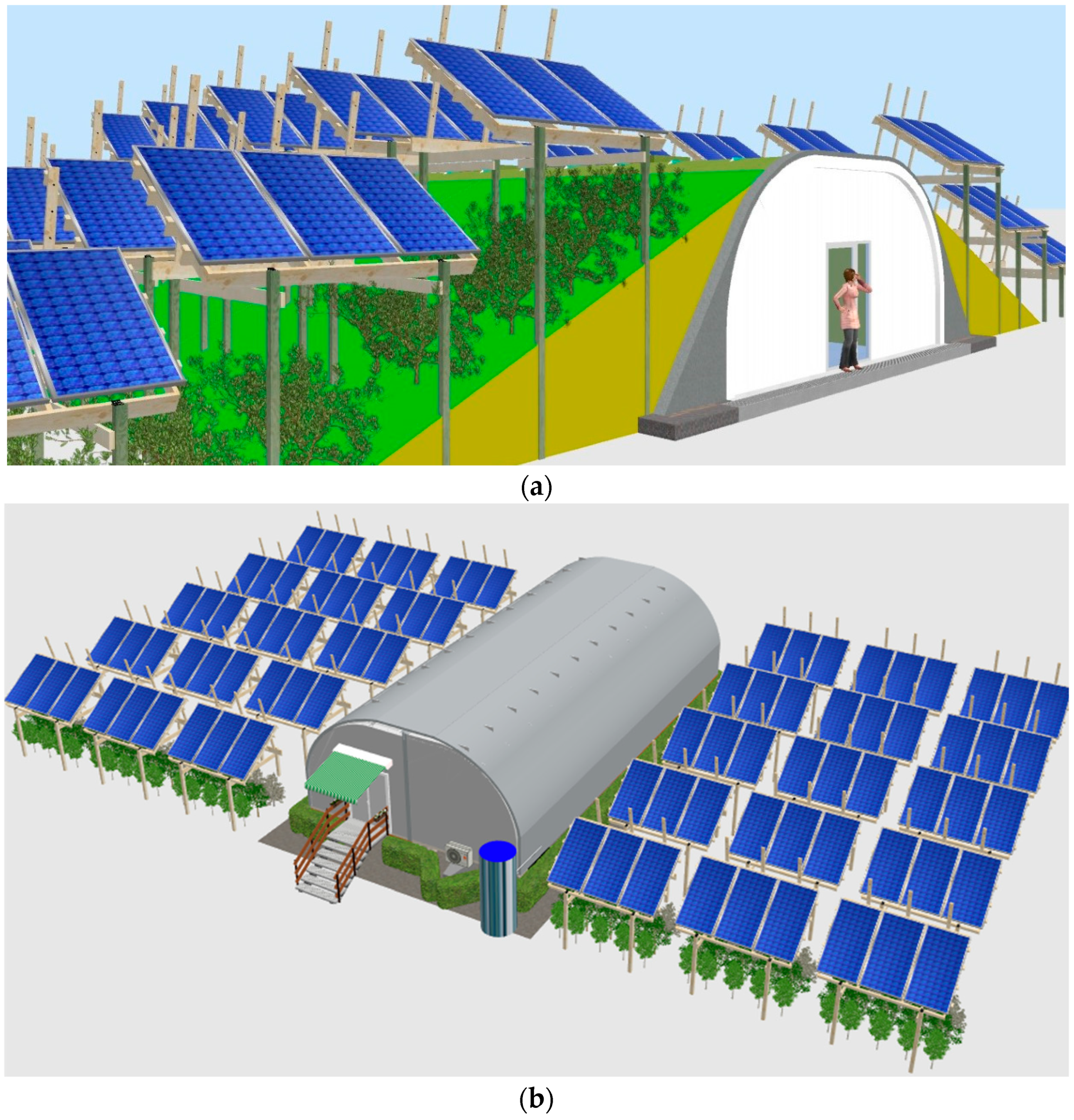
To overcome electrical costs for indoor farming, the agrivoltaics agrotunnel introduced here uses four approaches: (1) high insulation for a building dedicated to vertical growing, (2) high efficiency LEDs for lighting, (3) the use of heat pumps (HPs), and (4) to control the volatility and reduce the electricity costs, solar photovoltaics (PV) provide a known levelized cost of electricity (LCOE) and a 25-year lifetime. All these approaches have been combined in an agrivoltaics agrotunnel where agrivoltaics arrays on the outside provide power for the grow lights and water pumps and other electrical equipment on the inside. The core concept involves either an earth and vegetation-covered tunnel (Figure 1a) or a mobile unit (Figure 1b) housing high-density vertical aeroponic–hydroponic hybrid systems illuminated by high-efficiency LED grow lights. Next to the agrotunnel fixed/variable tilt agrivoltaics PV arrays [15] are shown, which provide all of the power necessary to operate the agrotunnel. Different types of agrivoltaics arrays could be used based on the type of outdoor crop coupled to the indoor production in the agrotunnel, such as conventional fixed tilt [16,17], stilt-based [18,19] systems, trellis systems [20,21,22], farm fence-based systems [23,24,25], single axis tracker [26,27] and fixed vertical [28,29,30] and dynamic vertical [31,32] arrays.
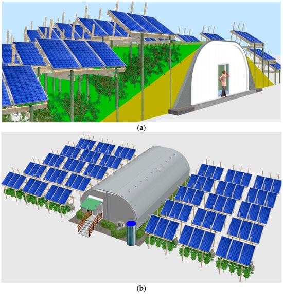
Figure 1.
Agrivoltaic agrotunnel: (a) subterranean agrivoltaic agrotunnel; (b) semi-mobile agrivoltaic agrotunnel.
PV technology has been declining in price for decades [33,34], making it the lowest-cost electricity generation technology [35,36]. This provides an opportunity to control the costs of indoor growing. Already because of this cost advantage, PV is the most rapidly expanding electricity source [37,38] and dominates new sources of power [39]. With the growth of PV, which demands large surface areas to provide large amounts of energy, there have been land-use conflicts associated with installing PV plants on farmland [40,41,42,43]. Fortunately, this can be rectified with agrivoltaics, which refers to the dual use of land for clean electricity generation with PV and agriculture [44,45,46,47,48]. This increases land efficiency [49,50] and agrivoltaic systems have proven to be economically viable as they provide farmers with dual stream of revenue—one through generation of electricity and one through the produce/crop yield [47,51,52,53,54,55]. To push this concept further, this paper investigates the potential of using agrivoltaics to power the even more land-use-efficient indoor growing inside an agrotunnel.
In order to size the net-zero agrivoltaics array that is necessary to support an agrotunnel, this study first develops a thermal model for load calculations in an agrotunnel, which has been validated using the results of a commercial building’s load calculation with the Hourly Analysis Program (HAP). Using measured data, the effect of plant evapotranspiration is included subsequently as it is not incorporated in HAP V 5.11 software. The size of heat pumps (HPs) needed to maintain a constant temperature in the agrotunnel is determined in the next step. Next, plug loads (i.e., water pump energy needed to provide for the hybrid aeroponics/hydroponics system, DC power running the LEDs hung on the grow walls, and dehumidifier assisting in moisture condensation in summer) are measured/modeled. Ultimately, all models are combined to establish an annual load profile for an agrotunnel (also verified based on two-month performance) that is then used to model the necessary PV to power the system throughout the year. The simulations of the developed model take place in Albany, Edmonton, Houston, London, Montreal, and San Francisco. The results are discussed, and future work is outlined to completely solarize agrivoltaics agrotunnels.
2. Agrivoltaic Agrotunnel
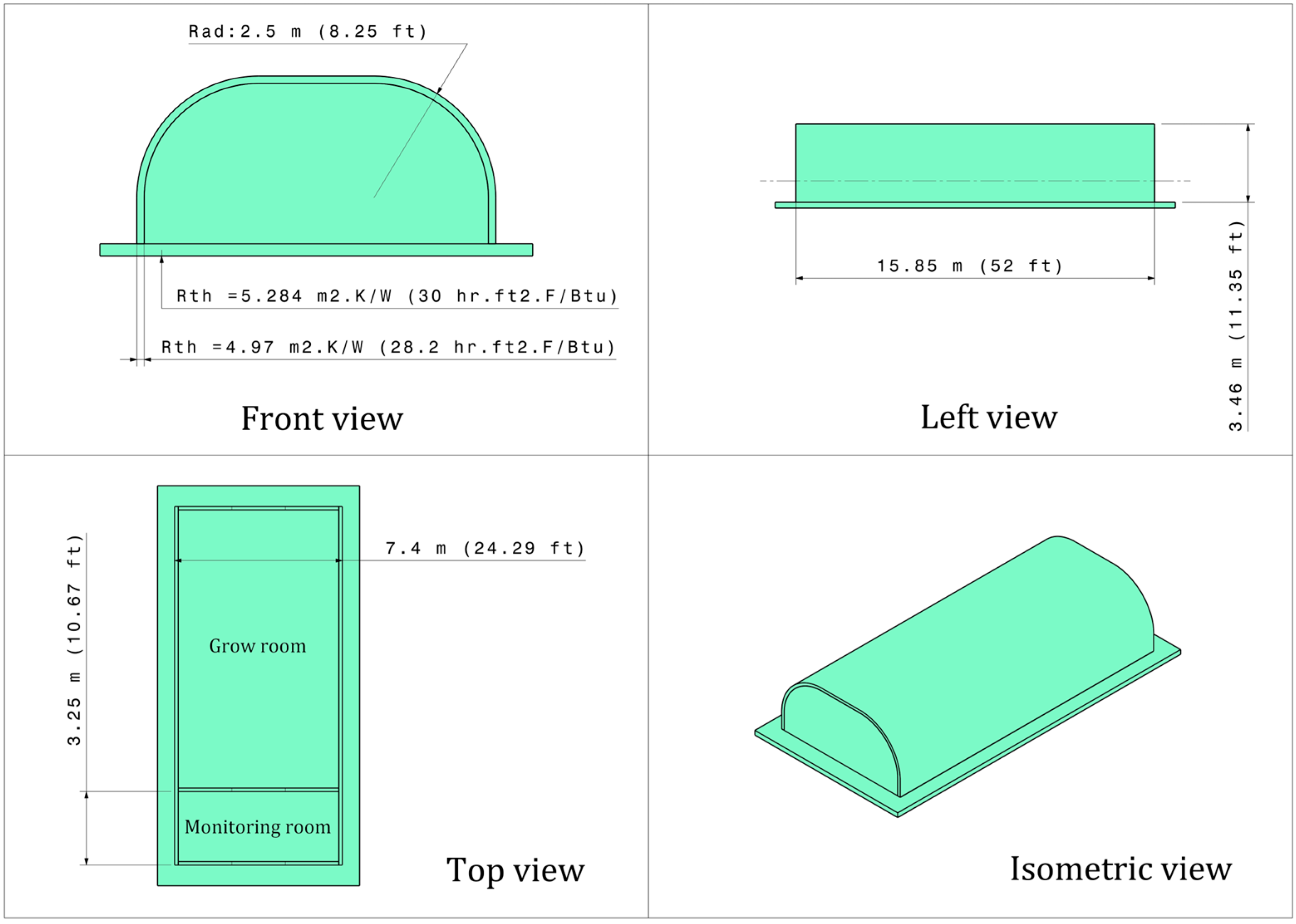
The agrotunnel (Food Security Structures Canada (FSSC) [56], London, ON, Canada) presents a solution to combat food insecurity by offering an easily assembled, scalable, and sustainable indoor vertical farming structure. It is designed to withstand extreme climate conditions and can be adapted to various locations. FSSC uses fiber reinforced polymer (FRP) construction to enhance its portability, strength, and its lightweight design to reduce the embodied energy and emissions for transportation. This innovative growing chamber enables precise control of light, humidity, and temperature, facilitating year-round cultivation of hybrid-aeroponic fruits and vegetables in harsh environments. Assembling the 1.2 m × 2.4 m panels allows for easy transportation of components. The detailed dimensions and thermal resistances of the agrotunnel envelope are illustrated in Figure 2.
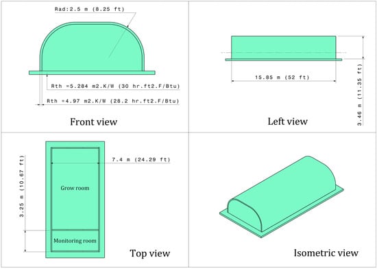
Figure 2.
The CAD model including the dimensions and the thermal resistances of the envelope.
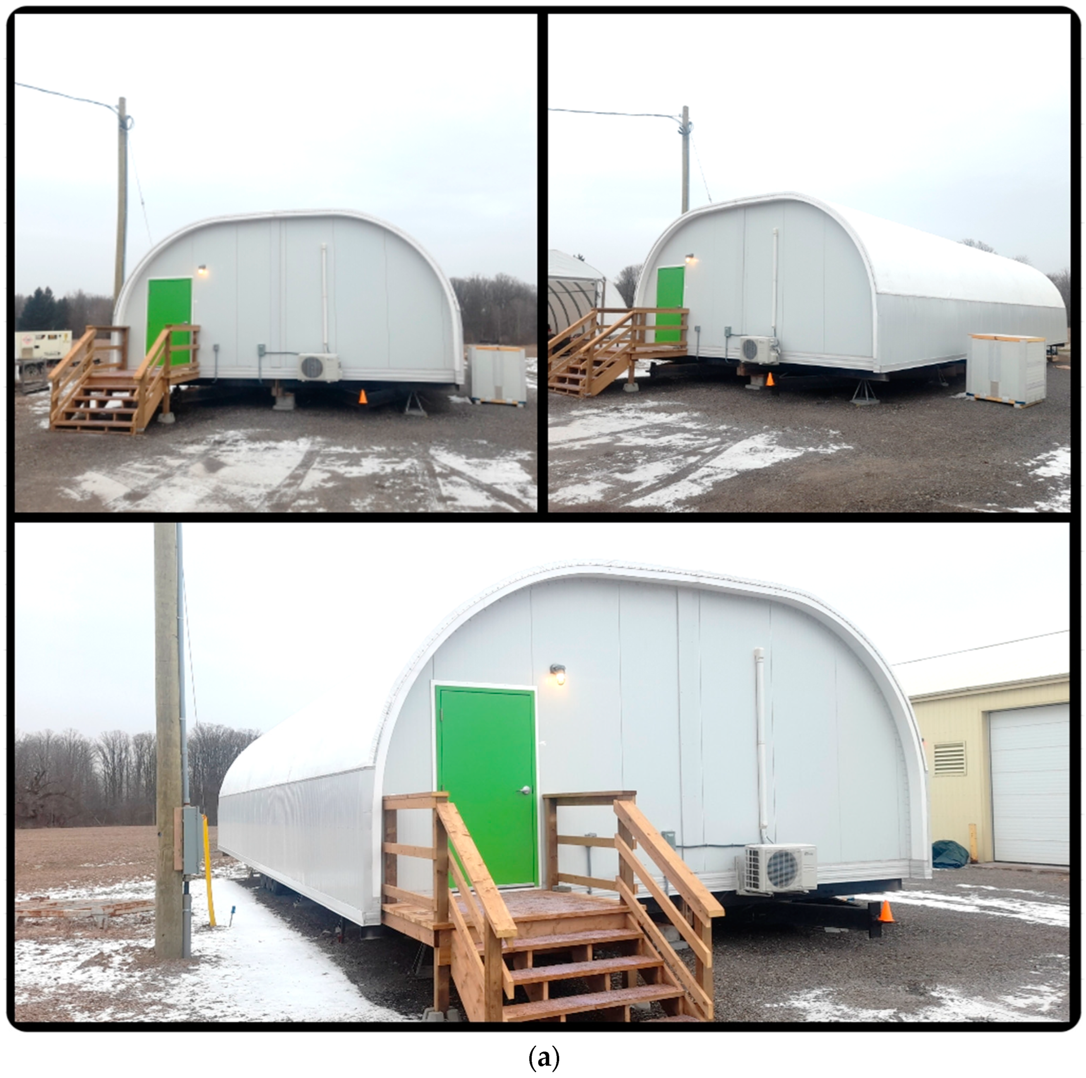
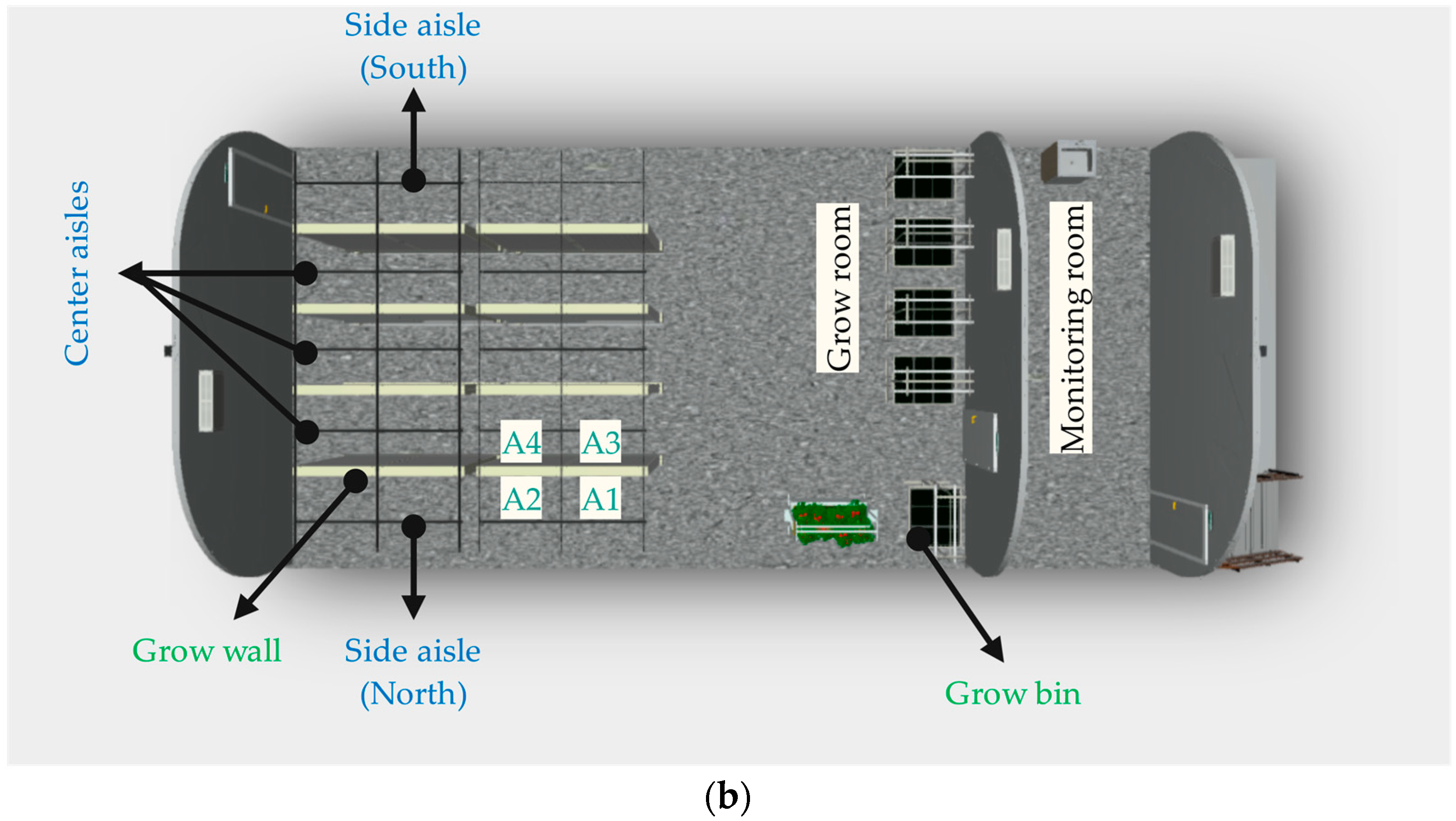
The agrotunnel under study is located at the Western Innovation for Renewable Energy Deployment (WIRED) in London, ON, Canada (Figure 3a). As shown in Figure 3b, the design is composed of two sections (grow room and monitoring room). Eight grow walls, each with two sides and two mini walls for each side, are installed in the growing room in addition to six grow bins. Utilizing the same growing technology as the grow walls featuring adjustable lighting brackets, the grow bins offer an ideal growing setting for root vegetables and other plants that demand greater space.
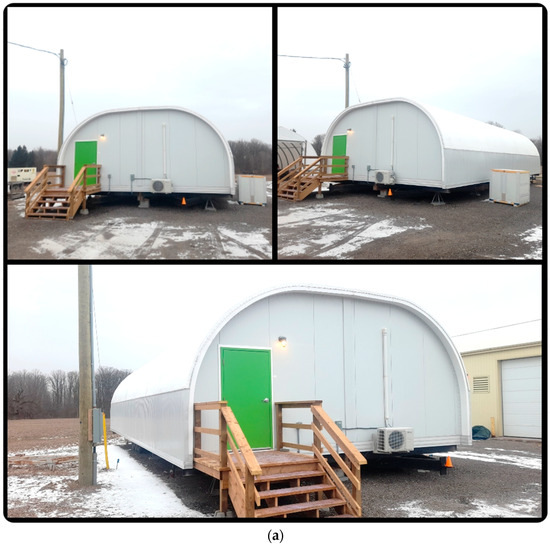
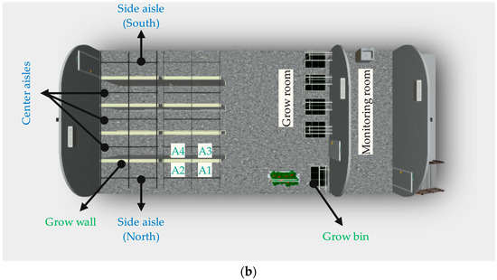
Figure 3.
The agrotunnel under study: (a) actual structure established at WIRED; (b) detailed model (top view).
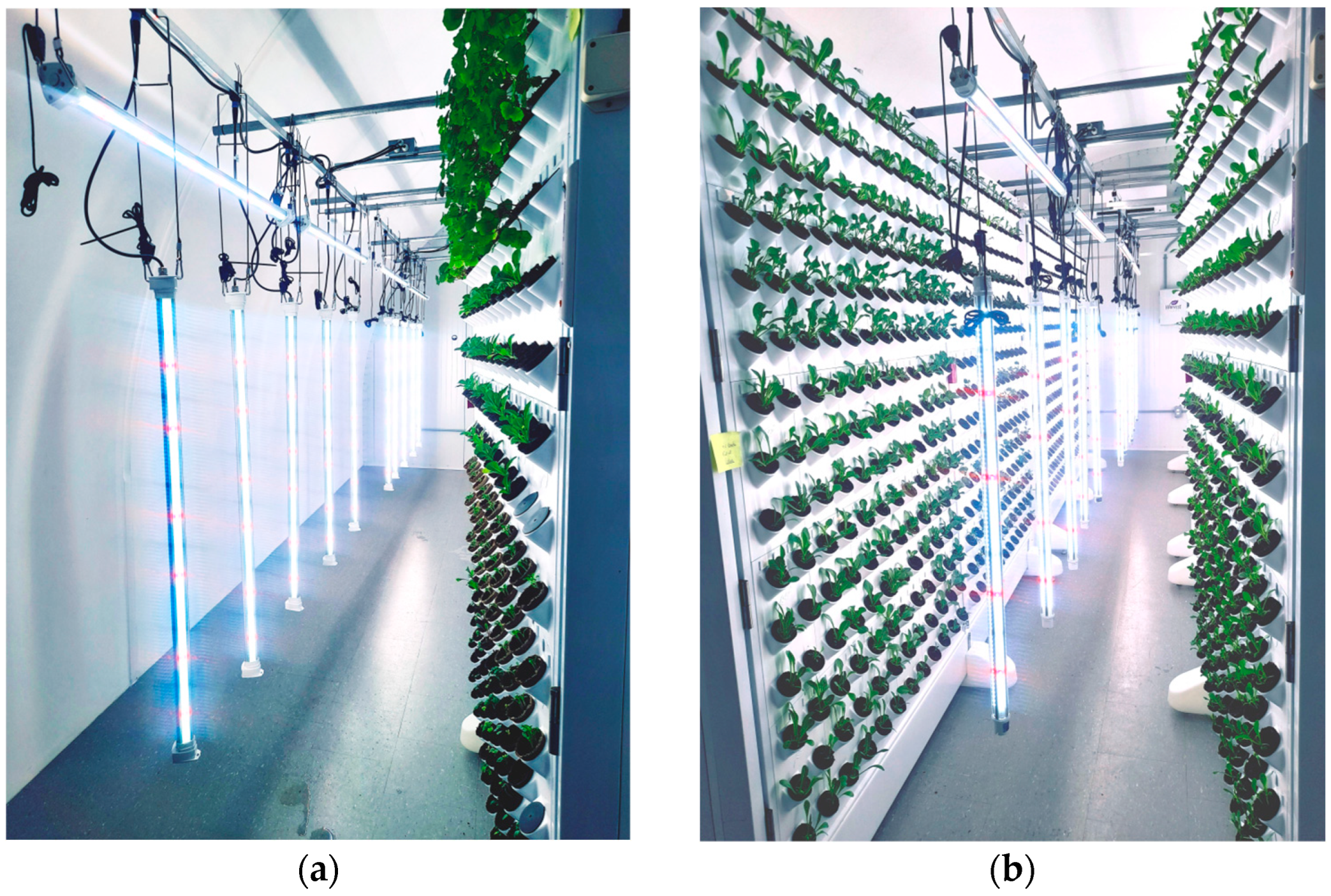
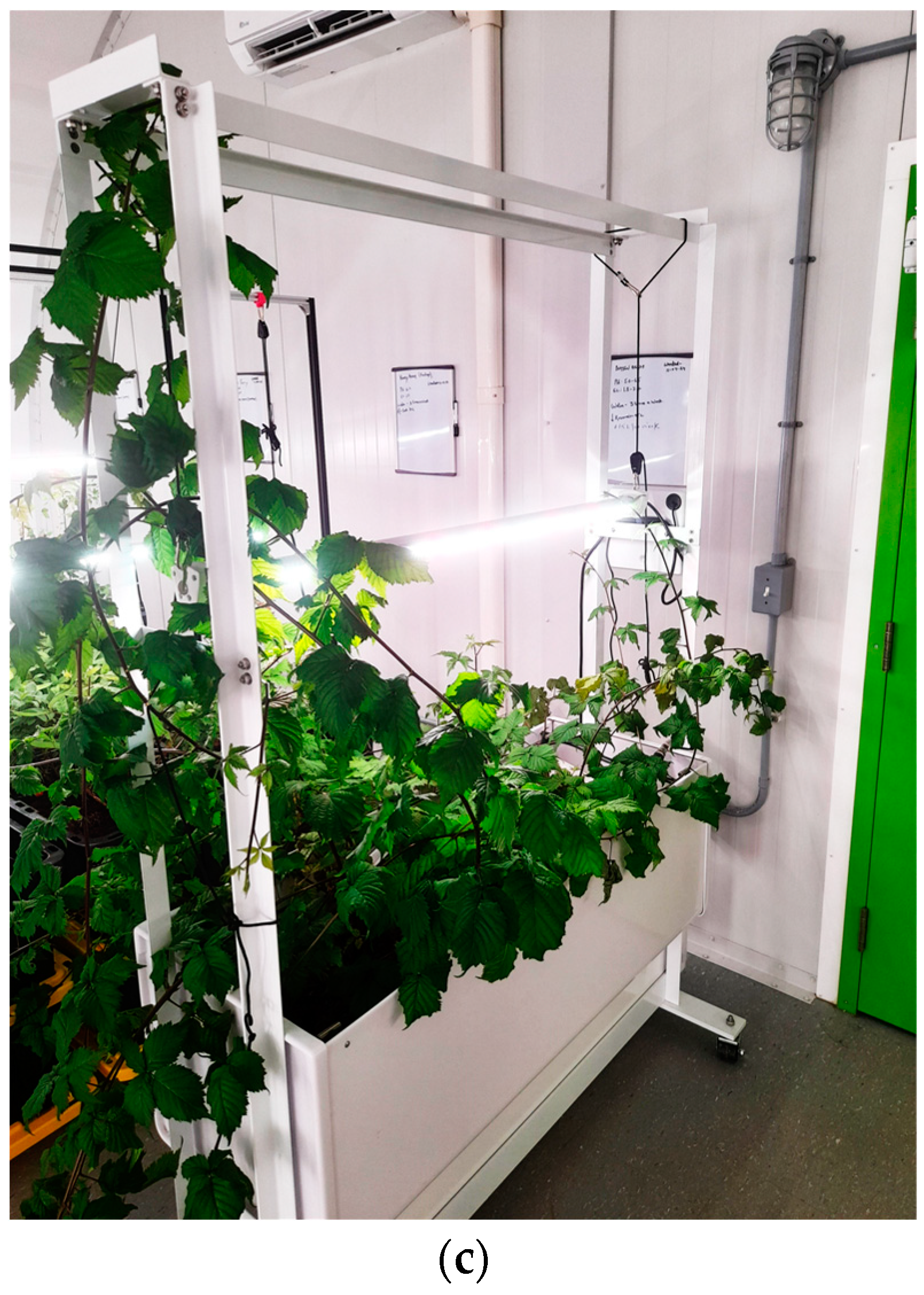
All the growing facilities are fed by low wattage and low voltage LED lights produced by Better Grow Lights [57]. These commercial lights are specifically designed for high density plant spacing and come with three 180° (BGL180A), 180° (BGL180C), and 360° (BGL360A) designs. BGL180A lights are hung on the side aisles as well as top of the grow bins, and BGL360A are hung on the center aisles, as shown in Figure 4. BGL180C are horizontally hung on top of the grow bins. In the agrotunnel, there are 28 BGL180A each with 75 W, 42 BGL360A each with 100 W, and 12 BGL180C each with 30 W wattage (11 in grow room and 1 in monitoring room).
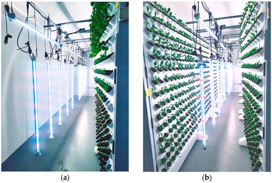

Figure 4.
The location of lights and their applications inside the agrotunnel: (a) BGL180A on the side aisles; (b) BGL360A on the center aisles; (c) BGL180C on the grow bins.
3. Methodology
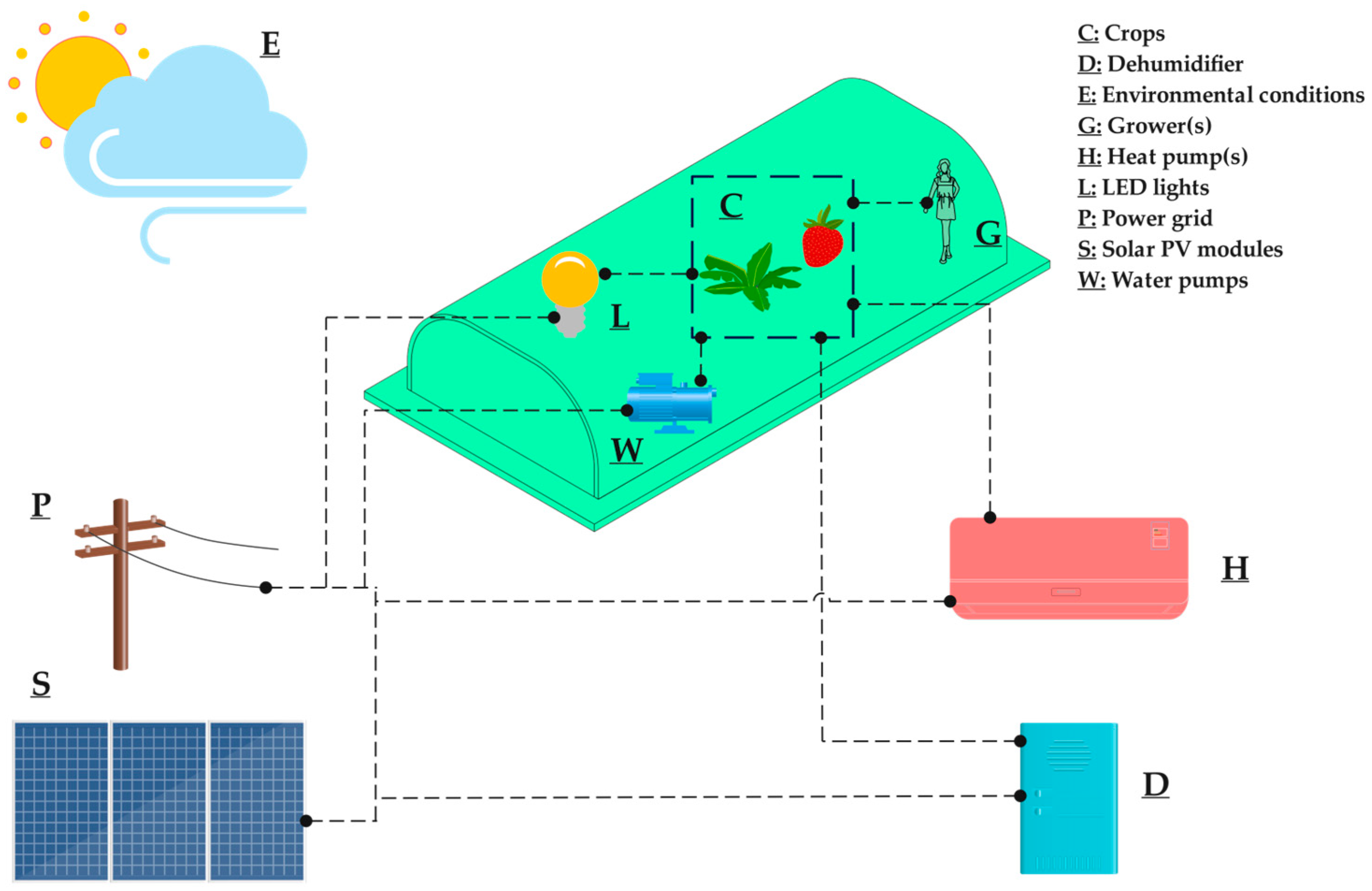
The agrotunnel’s load is made up of four sub systems: lights, water pumps, heat pump (HP), and a dehumidifier. A dehumidifier is operated to assist HPs in maintaining the relative humidity (RH) at a desired level. The HP is the major component in meeting the thermal (sensitive and latent) loads of the system. Artificial lighting also has a major contribution to increasing the temperature of the agrotunnel’s microclimate. All these loads are characterized as shown in Figure 5. Sizing all the thermal and electrical equipment would be done based on the loads as the results of the structure’s specifications and the circumstances the plants will grow under.
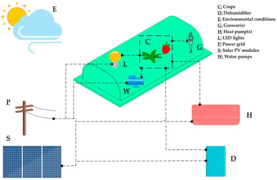
Figure 5.
Schematic of the agrotunnel integrated with the energy provision equipment.
3.1. Thermal Model
The load calculations of the agrotunnel are estimated using the following thermal model developed. It is assumed that all the lights are on and planted crops are mature enough. Meanwhile, one person is doing some non-strenuous work such as planting, harvesting, watering, etc. in the building. The following sub-models are developed based on the load calculation principles [58].
3.1.1. External Loads
CLTD/CLF method, described in the 1997 AHSRAE Fundamentals [59], is used to calculate the transmission load of the agrotunnel, which is the most practical method for sizing the HVAC equipment while being simple.
Equation (1) is used for calculating the heat gains through the walls, the roof, and the floor. Cooling load temperature difference (CLTD) considers the collective impact of variations in indoor and outdoor temperatures, daily temperature fluctuations, solar radiation, and heat retention within the building structure. The values are determined using the tables provided in Chapter 28 of the ASHRAE Fundamentals Handbook [59].
where represents the heat losses due to the conduction and convection transmission through the envelope. is the surface area of each part of the envelope (m2 or ft2) except for the floor and stands for the surface area of the floor. corresponds to the conduction and convection thermal resistance of each part of the envelope (m2·K/W or h·ft2·F/Btu), which can be calculated by Equation (2) [60]:
and are the indoor design temperature and the outdoor temperature (°C or °F), respectively. As the ASHRAE tables offer hourly CLTD values based on a standard scenario, such as an outdoor maximum temperature of 35 °C (95 °F), mean temperature of 29.44 °C (85 °F), and a daily temperature range of 11.67 °C (21 °F), Equation (1) is modified through Equations (3)–(5) to accommodate correction factors for situations deviating from this base case. CLTD values of the base case for the material used in the envelope are tabulated in Table 1 [59].
where the daily range of temperature (DRT) indicates the difference between the maximum and the minimum temperature within 24 h. For the floor transmission, () will be simply used.

Table 1.
CLTD values of the base case for the material used in the agrotunnel’s envelope [59] *.
The sensible and latent loads caused by infiltration can be calculated using Equations (6) and (7), respectively:
where is the total volume of the agrotunnel (m3 or ft3). and are the air density (kg/m3 or lbm/ft3) and specific heat capacity (kJ/kg·K or Btu/lbm·F), respectively. indicates the infiltration rate in ACH (h−1), which usually is 0.25 for a newly constructed and well-insulated building [61]; for this specific building without any windows and completely sealed walls, however, 0.1 will be a rational assumption. Also, and denote the indoor and outdoor humidity ratio in (kgw/kgda or lbm,w/lbm,da), respectively, and corresponds to the enthalpy of vaporization of water in (kJ/kg or Btu/lbm).
3.1.2. Lights
The waste heat dissipated by the LED lights mainly depends on their power and the cooling load factor (), which can vary within a day based on the operating schedule of lights. would be 1 for the case lights are on for 24 h. Otherwise, Table 2 will be used for one story building [59].
Table 2.
Cooling Load Factor (CLF) for lights [59] *.
Equation (8) gives the waste heat dissipated by lights in (W or Btu/h). , , , and are the number of lights used, the power of lights used in (W), the lights use factor, which can be assumed to be 1, and the ballast allowance factor, which can be assumed 1 for LED lights [62], respectively.
3.1.3. People
Each person working in an agrotunnel brings in both sensible and latent loads. Sensible and latent heat gained by a person carrying out sedentary (standing or walking slowly) or some light work are 92.4 W (315 Btu/h) and 95.3 W (325 Btu/h), respectively [59]. Total cooling load caused by the presence of the people in agrotunnel can be calculated using Equation (9):
where represents the total number of people who are working in the agrotunnel, and stands for the cooling load factor of people, based on the number of hours they work each day. In the basic scenario in the present study, it is assumed that one person is working 8 h for 7 days a week from 9 a.m. to 5 p.m. Therefore, using Table 3, the will be extracted. includes either 0 or 1 to consider the effect of the grower’s presence.
Table 3.
Cooling Load Factor (CLF) for people [59] *.
3.1.4. Evapotranspiration of Plants
There are many models of evapotranspiration [63,64], which incorporate the effect of various parameters, interpretation of which is beyond the scope of this study. In this case, the structure was designed with eight walls (each with 720 pots, totalizing 5760 pots); all are watered aeroponically at potentially different stages of growth and different species present an enormously complicated system. A more straightforward way to estimate the evapotranspiration load in a grow room involves calculating the net water consumption of plants. This entails measuring the volume of irrigation water introduced into the agrotunnel and subtracting the volume of water drained away [65]. The average amount of water consumed () can be estimated in kg/s or lbm/h. Hence, the heat of vaporization will be calculated using Equation (10):
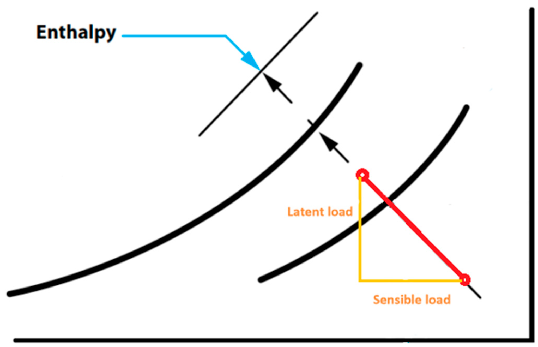
During this process, the moisture of the soil and the plants’ leaves absorbs heat from the environment, causing a temperature drop (sensible heating load) and then evaporating. The energy absorbed is converted to latent heat of vapor in the air, which causes an increase in the humidity level of the microclimate (the latent cooling load). This transfer in energy leads to a constant enthalpy process, which is shown in Figure 6.
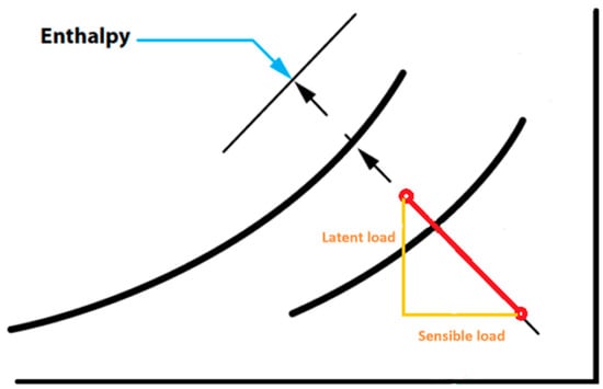
Figure 6.
The isenthalpic process of evapotranspiration that takes place in humid air.
Total sensible and latent thermal loads of the agrotunnel will be calculated using Equations (11) and (12), respectively.
The following assumptions are considered to run the simulation:
- It is assumed that the growing room and the monitoring room are at the same temperature such that no heat transmission occurs between them.
- It is assumed that the air inside the agrotunnel is uniformly mixed, which is appropriate as the HP locations and clearance over the grow walls ensure paths of airflow.
- The design conditions of the agrotunnel are the temperature of 22 °C and the relative humidity (RH) of 68%.
- The thermal resistance of the still air () on the vertical walls is 0.12 m2·K/W [61].
- The thermal resistance of the still air () on the ceiling is 0.11 m2·K/W whenever the indoor temperature is higher than the outdoor temperature, and is 0.16 m2·K/W when the indoor temperature is lower than the outdoor temperature [61].
- The thermal resistance of the still air () on the floor is 0.16 m2·K/W whenever the indoor temperature is higher than the outdoor temperature, and is 0.11 m2·K/W when the indoor temperature is lower than the outdoor temperature [61].
- The thermal resistance of the outdoor moving air () is 0.029 m2·K/W [61].
3.1.5. Maximum Heating Load Model
In order to size HP, the maximum cooling load obtained by the CLTD method will be compared to the maximum heating load under the worst-case scenario. The worst-case scenario for heating load estimations is defined for an evacuated agrotunnel, where conduction and convection heat transfer along with the infiltration losses are the only factors included. Total sensible heat loss from the agrotunnel is calculated by Equation (13) in W or BTU/h [61]:
Total latent heat loss through infiltration is calculated using Equation (7). Accordingly, the maximum total heating load will be calculated by Equation (14):
3.2. Heat Pump Model
The black box heat pump model is created by utilizing the performance datasheet of GSZ16 Goodman Air-to-Air Split heat pump (16 SEER and 9 HSPF) for both heating and cooling functions [66]. A supervised regression approach is implemented in Python to derive mathematical functions for the COP (Coefficient of Performance) of heat pumps within a nominal capacity range of 18,000–60,000 BTU/h. Drawing from Li et al.’s correlations for load demand and COP of an air-conditioning heat pump [67], it is anticipated that the COP regressions would follow a second-degree polynomial pattern based on indoor and ambient temperatures.
3.2.1. Heating Mode
The correlation of COP is dependent on the ambient temperature () in (°C) as Equation (15):
where the coefficients are extracted using the polynomial curve fitting technique and are shown for all rated capacities of GSZ16 Goodman Heat Pumps in Table 4 for heating mode. The fitting curve of heating COP for 18,000 BTU/h heat pump is shown in Figure 7a.
Table 4.
Coefficients of polynomial correlations of COP in heating mode.
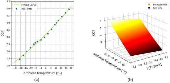
Figure 7.
Fitting curves of COP for 18,000 Btu/h heat pump: (a) heating mode; (b) cooling mode.
3.2.2. Cooling Mode
The manufacturer’s datasheet for cooling mode was created considering fluctuations in 3 variables (ambient temperature, indoor dry bulb temperature, and indoor wet bulb temperature) [66]. Hence, the regression is carried out in two steps: first, fitting a 2D curve as a function of indoor dry bulb and wet bulb temperatures; second, fitting a 3D surface as a function of first formulation and the outdoor temperature. Figure 7b depicts the fitting surface for the COP of an 18,000 Btu/h HP in cooling mode. The COP for the cooling mode is determined using Equation (16). The coefficients are shown for all rated capacities of GSZ16 Goodman Heat Pumps in Table 5 for cooling mode.
Table 5.
Coefficients of polynomial correlations of COP in cooling mode.
When the maximum heating and cooling load of the agrotunnel on the coldest/warmest day of the year is calculated, the size of HP can be determined. After selecting the HP, its COP correlation is used to calculate the power consumption in kW.
3.3. Electrical Loads
The power demanded by the lighting system and the HPs can be calculated as mentioned in the previous section. The load imposed by the water pumps and dehumidifier is included in this section.
3.3.1. Water Pump
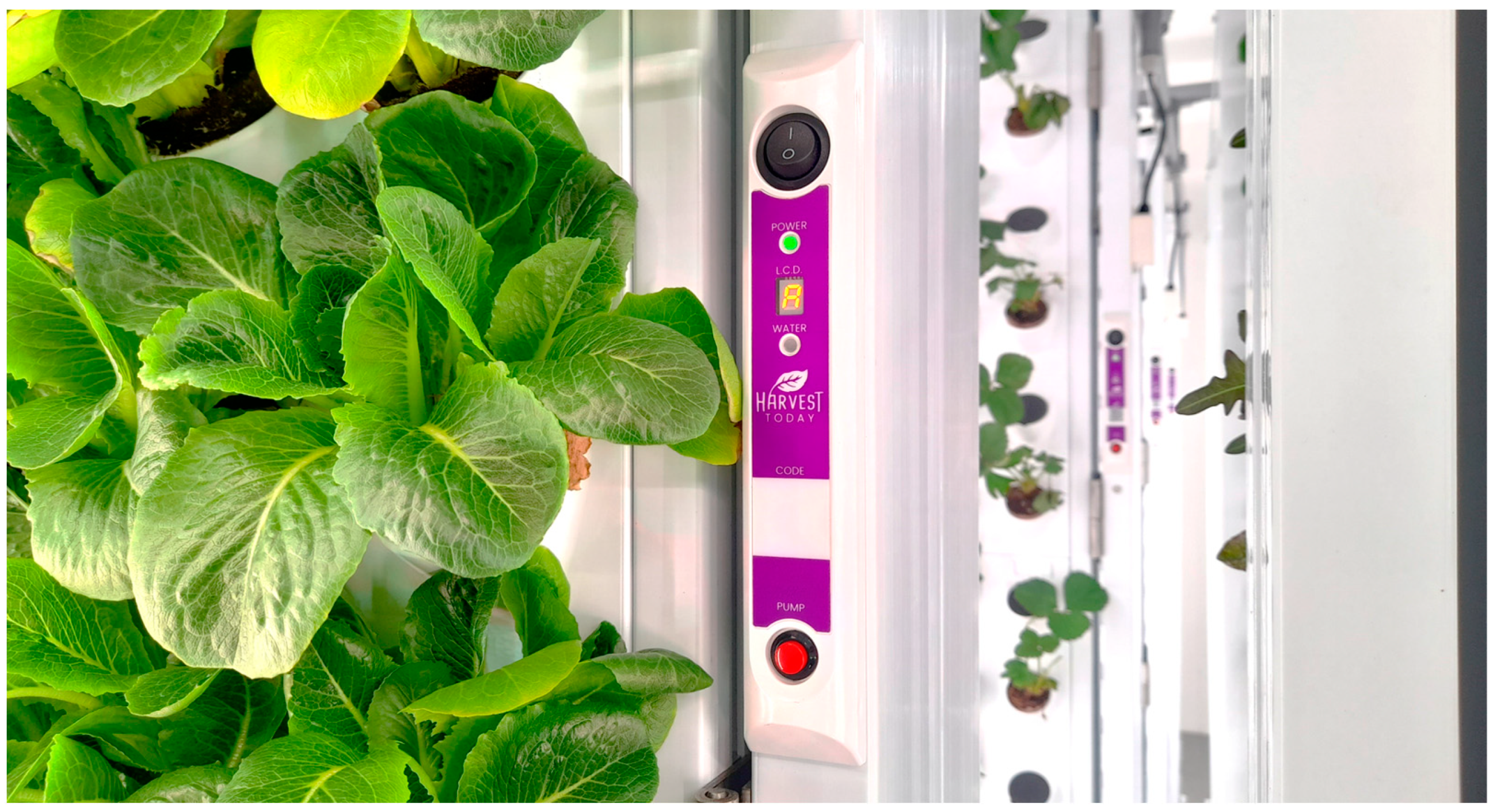
Water pumps are integrated into the grow walls, and they operate 2–4 times per day (1–2 mins each time) based on the requirements of the plants according to their stage (seedlings or mature) (Figure 8). Therefore, the average power consumption of water pumps is reported based on the data recorded by clamp meter [68]. The average power demand by the water pumps is 0.038 kWh.
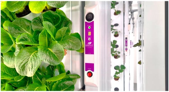
Figure 8.
Water pump integrated into the grow wall.
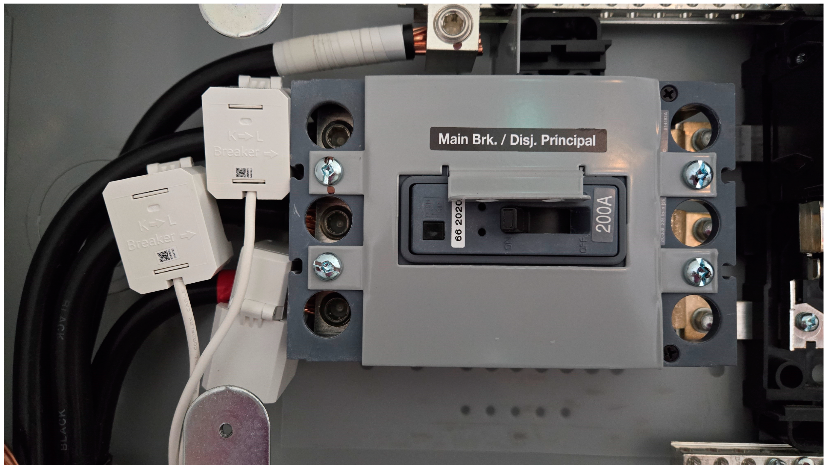
The power consumption data for the agrotunnel were measured using the Emporia Energy Vue 8 Smart 3-Phase Gen 2 Home Energy Monitor manufactured by Emporia Renewable Energy Corporation, CO, USA [68], although an open source meter could be used [69,70]. The Energy Vue meter is capable of measuring current up to 200 A from the mains. The electrical breaker panel is a 200-A, 3-phase panel. The three main clamps are connected to the three hot wires coming from the grid to the panel (Figure 9).
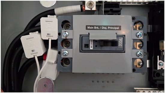
Figure 9.
Three main clamps connected to the main hot wires coming from the power grid to the agrotunnel’s circuit breaker box.
3.3.2. Dehumidifier
A commercial 23.7 L/day (50 pits/day) refrigerant dehumidifier [70] with the integrated energy efficiency (IEF) of 1.9 L/kWh is used in cases the heat pump cannot meet the latent load inside the agrotunnel [71]. Based on previous work it is assumed that if the latent load of the agrotunnel is higher than one third (which can be usually provided by HPs) of the maximum sensible load, the rest will be met by the dehumidifier [72]. To be conservative, it is considered that all the grow walls are filled with mature plants. Table 6 reports the average water added to each pot of a mature plant during a week, which is measured in an agrotunnel similar to the one under study [73]. In the basic scenario, it is assumed that all pots are equally allocated for planting four types of crops with the cultivation time (seeding to first harvest time) of 6–7 weeks, 4 weeks, 6–8 weeks, and 4 weeks, respectively for kale, lettuce, herbs (specific types only), and fruits and vegetables (specific types only).
Table 6.
Water demand of the mature crops in the agrotunnel (per pot per week).
3.4. Solar PV Sizing
PV system sizing was carried out by determining the 1-kW PV potential using the open-source System Advisor Model (SAM) [74] for each of the six locations: Albany, Edmonton, Houston, London, Montreal, and San Francisco. Using the total annual electrical energy required for agrotunnel operation (, in kWh) in each location and the annual energy potential of 1-kW PV system determined from SAM (, in (kWh)), the total PV system size () required to meet the annual electrical load is ascertained. The formula for determining the PV size in (kW) is given by Equation (17):
The PV system capacity determined through the estimate calculation is then used as input in SAM to run a detailed simulation at the appropriate scale. The simulations are run for each location and double checked if they meet the annual electrical load of the agrotunnel. Additionally, the land area required for PV systems, considering their modules’ transparency levels ranging from 0% (conventional silicon modules) to 69% (semi-transparent modules) will be reported. Table 7 details the assumptions used to perform the final modelling in SAM. A novel fixed-tilt racking design, adaptable into a variable-tilt racking system [15], is considered for use in this research. Soiling losses, DC power losses, and AC power losses are kept as default.
Self-consumption (SC) and self-sufficiency (SS) are important metrics for assessing the energy performance of distributed energy systems at the local level [75]. SC measures the proportion of locally produced energy that is consumed locally, calculated as the energy generated by the PV system () minus the energy sent to the grid (), divided by the total energy generated by the PV system () as seen in Equation (18). SS, on the other hand, indicates the extent to which local energy production meets local energy demand, calculated as the energy generated by the PV system minus the energy sent to the grid, divided by the local energy consumption () (Equation (19)). Both metrics exclude nighttime hours when the PV system is not operational, and all energy is sourced from the grid, thus SC and SS are set to zero during these times. These metrics can be formulated through Equations (18) and (19) [76,77].
Table 7.
Input parameter for SAM for PV system sizing for the agrotunnel.
Table 7.
Input parameter for SAM for PV system sizing for the agrotunnel.
| Parameters | London | Albany | Edmonton | Houston | Montreal | San Francisco |
|---|---|---|---|---|---|---|
| PV module | Heliene 144HC-460 Bifacial [78] | |||||
| Module type | Mono Crystalline Silicon—Bifacial | |||||
| Tilt angle | 34° [31] | 34° [79] | 53° [80] | 27° [81] | 30° [82] | 32° [83] |
| Azimuth | 180° | |||||
| Soiling losses | 5% | |||||
| DC power losses | 4.44% | |||||
| AC power losses | 1% | |||||
3.5. Data Presentation
The outcomes of the current study will be presented in the following section, starting with the analysis of the thermal and electrical loads of the agrotunnel across six locations. Next, the sensitivity of the total thermal and electrical loads to various influencing factors will be examined and presented. Subsequently, the results of PV sizing for the six locations will be detailed, followed by a performance analysis of the PV system specifically for London, ON. A comprehensive discussion will be provided in Section 4.
4. Results
The assessment of thermal loads will account for the impact of various geographical locations, including London, ON, Canada; Montreal, QC, Canada; Edmonton, AB, Canada; Albany, NY, USA; San Francisco, CA, USA; and Houston, TX, USA. Additionally, a sensitivity analysis will be performed to examine the effects of key variables such as envelope thermal resistance, number of lights, crop type, and indoor design conditions.
4.1. Validation
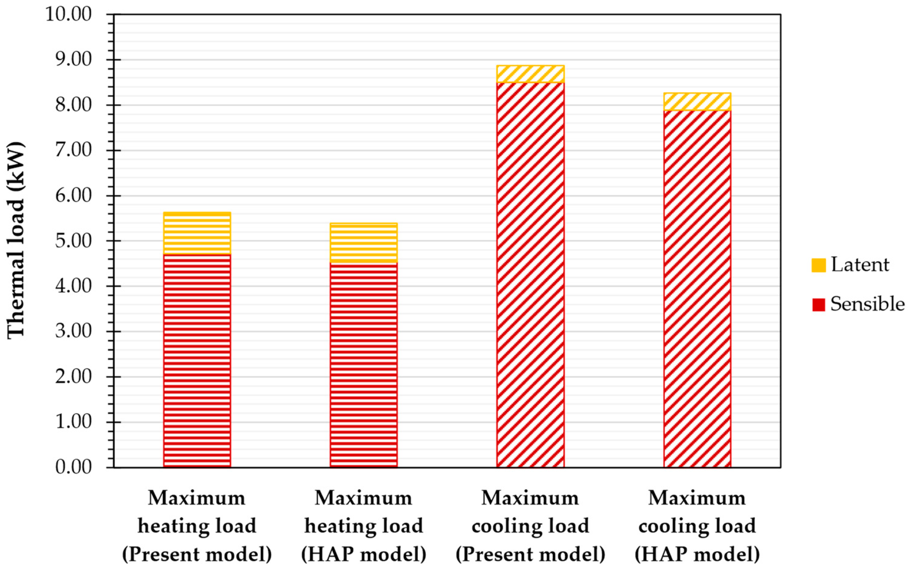
The methodology for both the CLTD and the maximum heating requirement model is validated against the results obtained from HAP. For the minimum dry bulb and wet bulb ambient temperatures of −19.4 and −20.22 °C, respectively, and the maximum dry bulb and wet bulb ambient temperatures of 29.44 and 21.67 °C, respectively, the heating and cooling loads of the agrotunnel in London, Ontario, Canada will be obtained using the current model, as shown in Figure 10. The average deviation of calculated heating and cooling loads from the HAP simulation results is 5.0 and 4.3%, respectively. The present model provides more conservative results for sizing the HVAC systems.
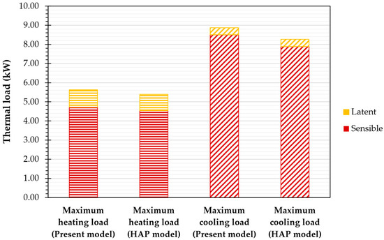
Figure 10.
The results of the present model vs. those of HAP model for calculation of heating and cooling loads.
Likewise, the HP model’s verification involves comparing it with the manufacturer datasheet of the GSZ16 series Goodman Air-to-Air heat pump. The average variance of the matched outcomes for heating COP with the manufacturer’s datasheet is determined to be 2.48%. Meanwhile, the average variance of the matched outcomes for cooling COP stands at 1.26%.
The total power demand of the agrotunnel has been verified using data recorded by a power clamp meter. Recording began in mid-February 2024, and as of mid-June 2024, data are available for March, April, and May 2024. March data, however, showed inconsistencies in both the climatic conditions of the agrotunnel and the data recording procedure. Therefore, the monthly power consumption of the entire system has been verified according to the conditions of April and May, reported in Table 8. Figure 11 illustrates the similarity between the modeling results and the recorded data, with an error ranging from 5.5% to 7.5%. The sources of error include real-world operational variations such as changes in planted crop types, RH setpoints, and the number of operating lights as experiments are adjusted. Additionally, temporary additions or removals of some equipment, such as water transfer pumps, contribute to these variations. Despite these factors, the current model tends to overestimate the total energy required, making it a more conservative estimate.
Table 8.
Conditions considered in the experimental verification of monthly total power demand.
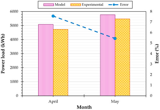
Figure 11.
Monthly power demand of the agrotunnel reported for April and May 2024 (modeling vs. experimental data).
4.2. Thermal/Electrical Load Analysis
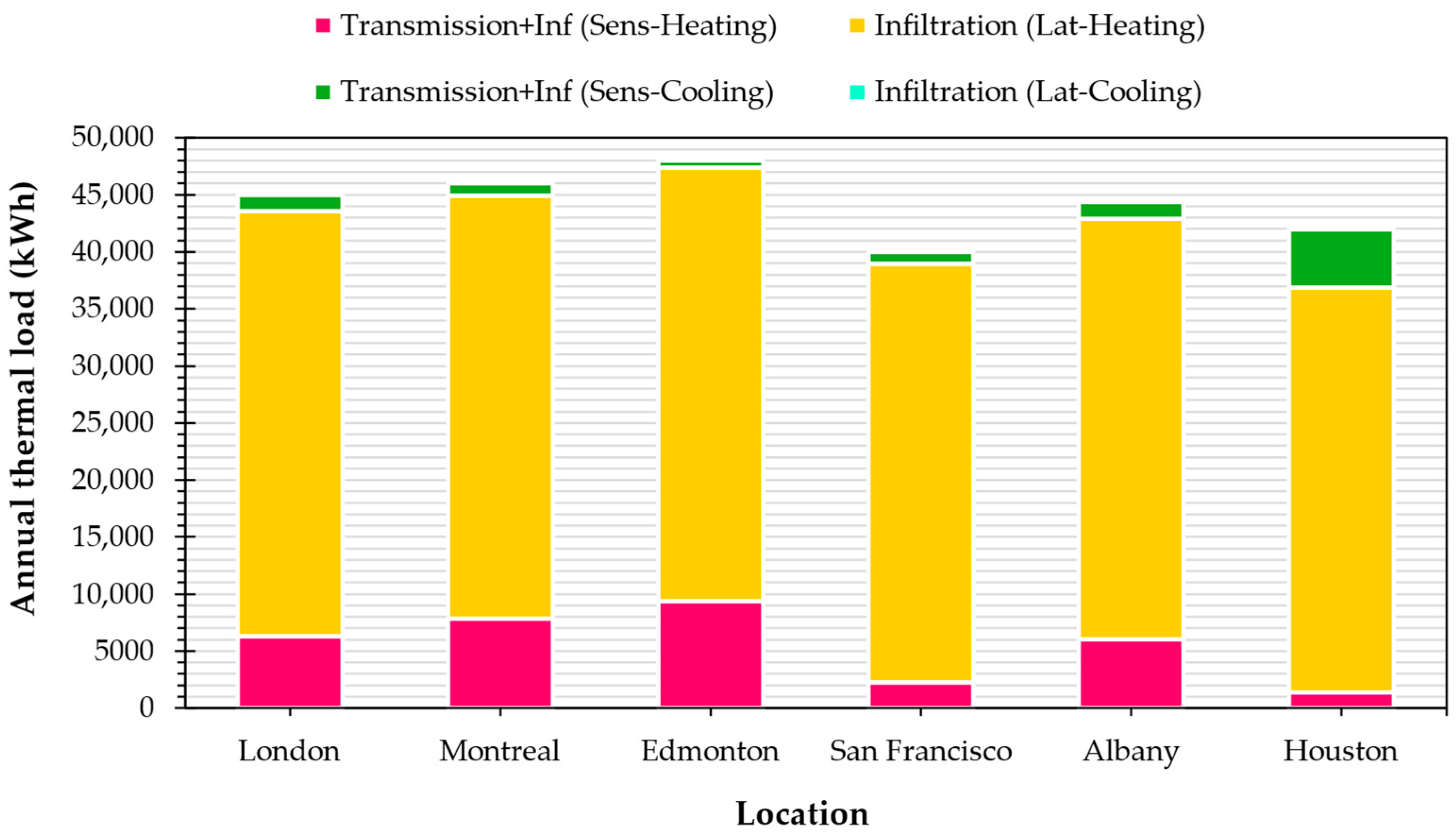
Initially, the year-round heating and cooling load of the agrotunnel is simulated based on the climatic conditions of the six selected case study locations. This section evaluates solely the sensible and latent loads induced by envelope transmission and infiltration, aiming to compare the impact of geographic location while disregarding constant thermal loads such as people, crops, and lights. Figure 12 illustrates the results of this comparison. Edmonton exhibits the highest total load (sensible heating load of 9370 kWh, latent heating load of 38,035 kWh, and the sensible cooling load of 603.5 kWh), whereas San Francisco displays the lowest (sensible heating load of 2255 kWh, latent heating load of 36,680.5 kWh, and the sensible cooling load of 1050.5 kWh), which aligns with their distinct climates as expected. San Francisco’s climate during the year undergoes fewer fluctuations such that the microclimate of the agrotunnel located there will have the least deviation from the outdoor conditions. Cities with the highest sensible heating loads demonstrate the lowest sensible cooling loads, and vice versa. Notably, a significant portion of the load corresponds to latent heating resulting from the humidity ratio difference between the agrotunnel and the exterior. This underscores the importance of maintaining this humidity level as a crucial HVAC measure.
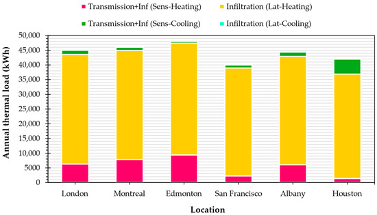
Figure 12.
Heating and cooling loads caused by heat transfer through the agrotunnel envelope and the infiltration.
Figure 13 illustrates the proportion of each heat transfer component of the individual thermal loads in an agrotunnel located in London, ON. It is evident that lights account for 40% of the thermal loads in the agrotunnel. Following closely, the evapotranspiration of plants places a substantial burden on the HVAC systems within the structure (32%). Sensible infiltration and wall transmission account for roughly a quarter of the load and finally the load imposed by the presence of the people has almost no impact.
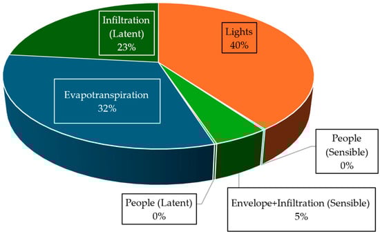
Figure 13.
Share of heat transfer components in the annual thermal load of the agrotunnel in London, ON, Canada.
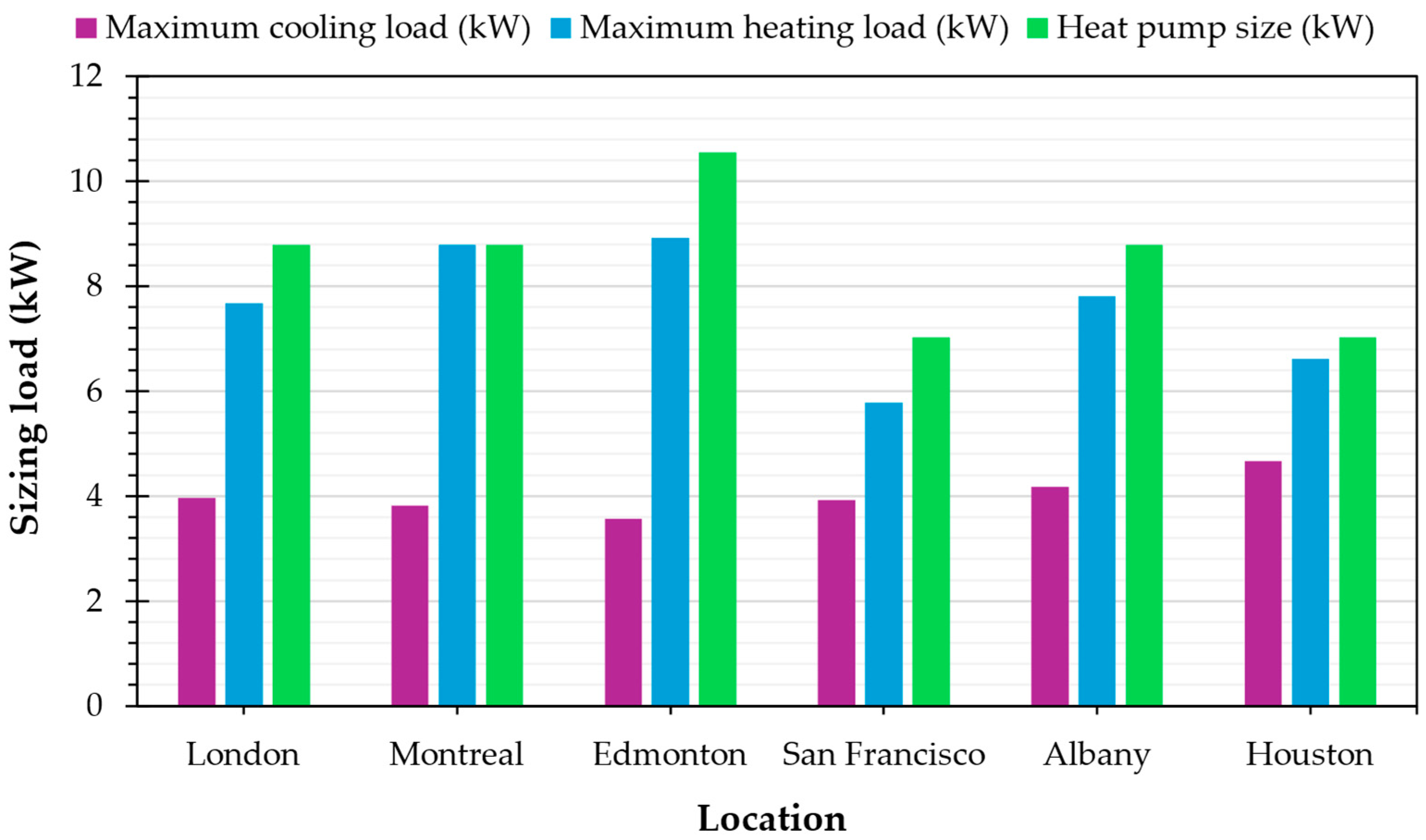
The heat pumps are sized and selected based on the worst-case scenario, encompassing either the maximum cooling or heating load within the building as illustrated in Figure 14. The considerable variance between the maximum heating and cooling loads, resulting in potential oversizing of the HP, is due to the definition of the worst-case scenario on the coldest day (evacuated agrotunnel devoid of plants and lights). This can be a subject for future deliberation in decision-making processes as it is only necessary to ensure heating to keep plants alive. The disparity between the heat pump’s size and the maximum heating load stems from commercially unavailable HP capacities. This indicates a market opportunity for more refined HP sizing to allow for closer optimizations. The largest HP capacity is designated for an agrotunnel situated in Edmonton (11 kW or 36,000 Btu/h), while the smallest is allocated for structures in San Francisco and Houston (7 kW or 24,000 Btu/h).
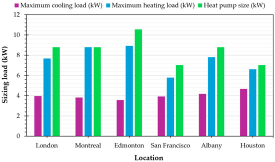
Figure 14.
The thermal load of the agrotunnel under worst-case scenario and HP sized to meet the maximum loads.
In the subsequent stage, Table 9 presents projections of the annual electricity required by four primary components: lights, HP, dehumidifier, and pumps, across three cities with varying levels of demand. Across all three locations, the highest power demand is attributed to the artificial lighting system, followed by the dehumidifier, with the pumps requiring the least power. In Edmonton, where the heating demand of the agrotunnel notably surpasses the cooling demand (as depicted in Figure 12), the HVAC system necessitates less power to cater to the cooling load of the structure. Additionally, the lighting system not only fulfills the heating requirement but also generates surplus cooling load, even on cold days. Consequently, the net value of HP power consumption during cold days is even smaller (2756 kWh, 4%). In conclusion, it can be argued that the colder the climate, the lower the predicted demand for the HVAC system within the current system design.
Table 9.
The annual electricity power demand of electrical equipment in the agrotunnel (kWh).
4.3. Sensitivity Analysis
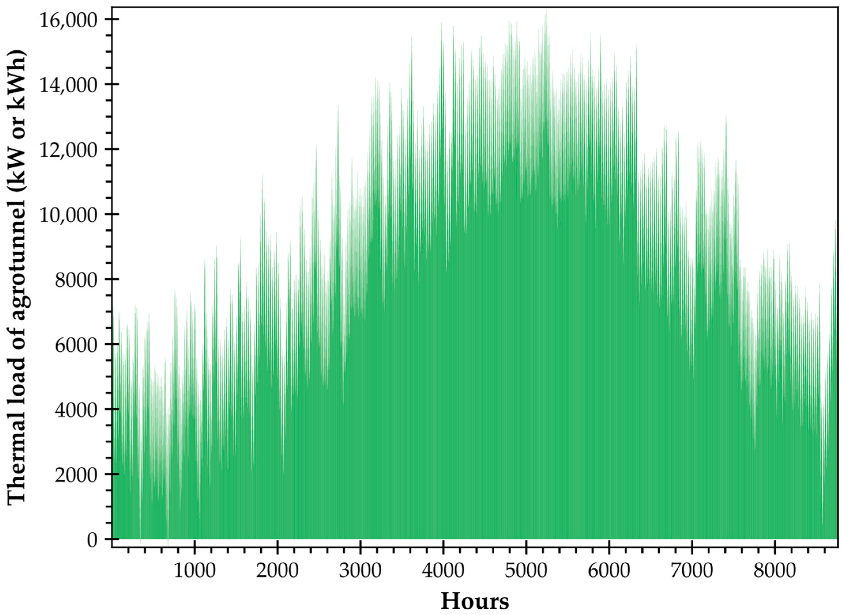
In this section, the sensitivity of two major energy indices (annual thermal load and annual power demand) are studied under the influence of the most significant parameter variations. The hourly thermal load requirements of the agrotunnel are first portrayed in Figure 15 for the year-round application. As a result of the continuous operation of lights, the building experiences a need for cooling throughout the year.
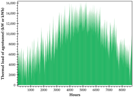
Figure 15.
The year-round hourly thermal load of the agrotunnel.
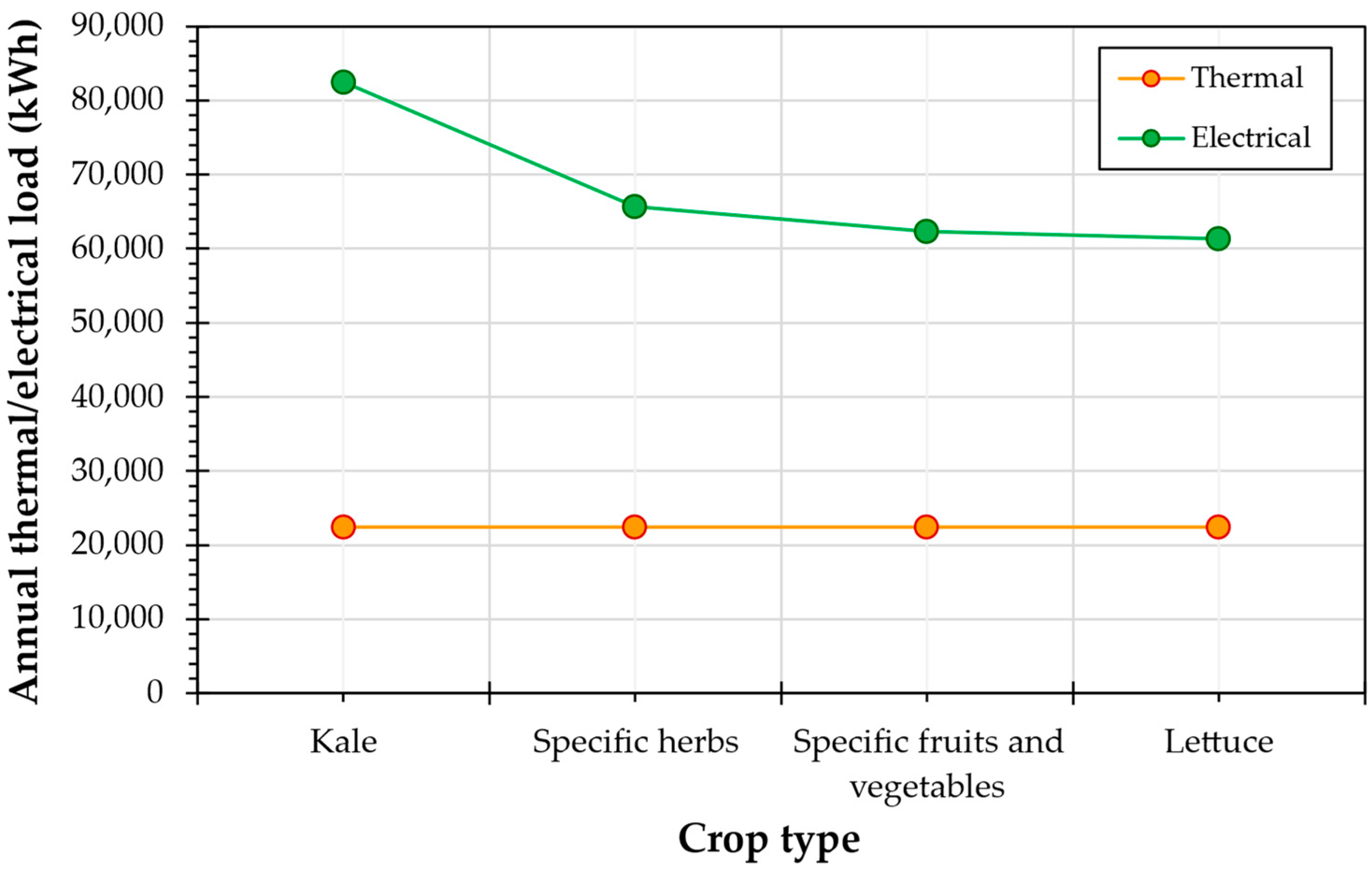
The choice of crop to be harvested in an agrotunnel greatly influences the water usage, as it directly impacts the evapotranspiration rate and consequently alters the load of the building. According to Figure 16, any variation in the evapotranspiration rate of the plants results in a consistent thermal load, as evapotranspiration is an isenthalpic process. There is, however, a reduction in power demand due to changes in the electricity consumption rate of dehumidifiers, resulting from a significant decrease in the latent load of the agrotunnel.
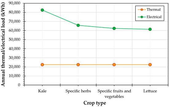
Figure 16.
Variation in annual thermal and electrical loads of the agrotunnel vs. change in crop type based on water use in grow walls for each specific crop type.
According to Figure 16, in an agrotunnel dedicated solely to growing kale, which requires more frequent watering cycles, there is a 25.53% increase in annual electricity demand compared to an agrotunnel for growing some specific herbs (from 65.46 to 82.42 MWh). This difference rises to 32.26 and 34.32% when compared to specific vegetables and lettuce, respectively.
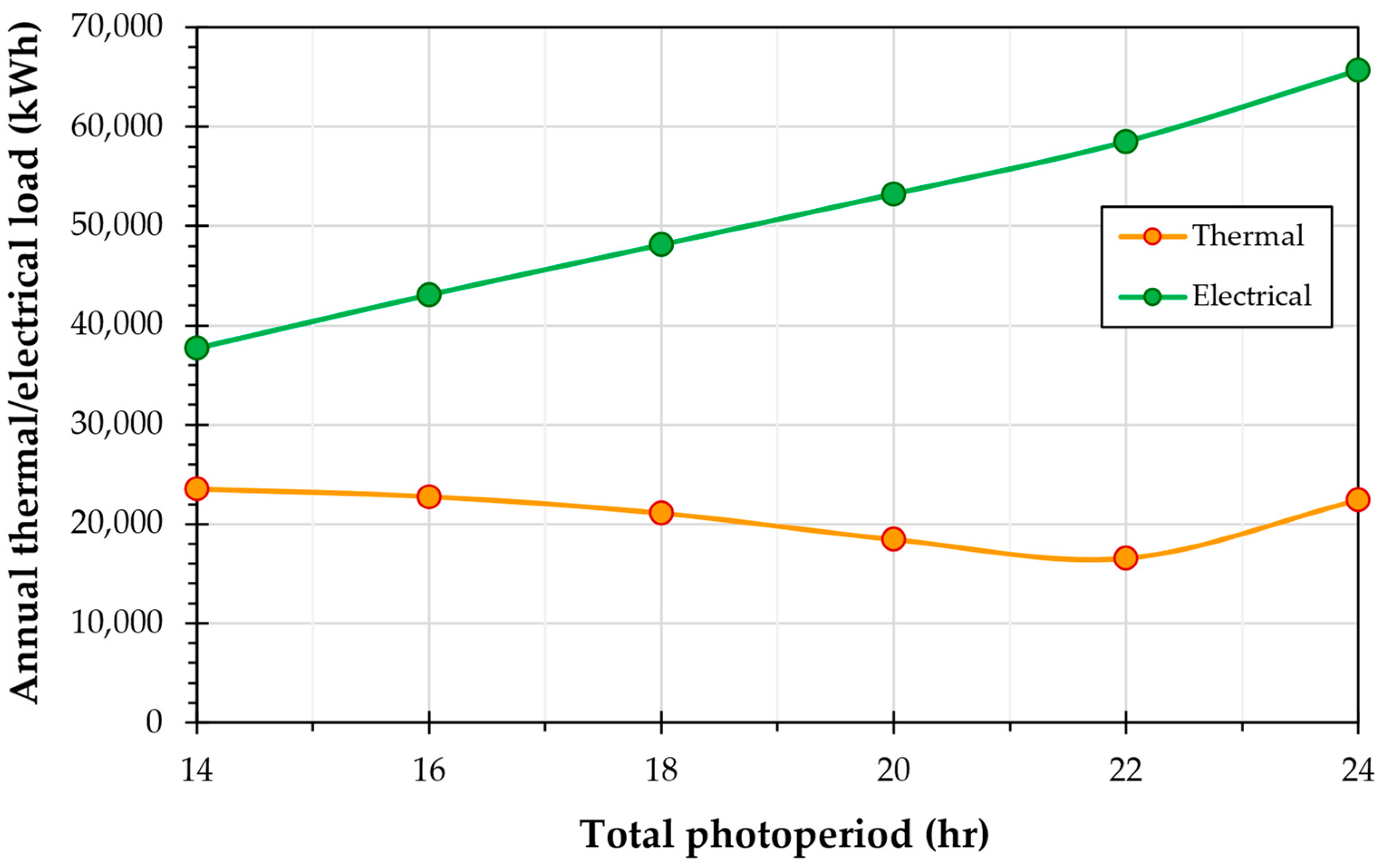
Figure 17 illustrates the variations in the annual thermal and electrical loads of the agrotunnel concerning changes in the photoperiod. Reducing the photoperiod from 24 to 14 h per day, a practice commonly applicable to many crops [85], results in a substantial decrease in the annual electrical load, dropping from 65,658 to 37,711 kWh, which was normally expected due to the reduction in the power load imposed by the lights. The annual thermal load, however, has a different trend. It decreases from 23,497 to 16,533 kWh with the reduction in the photoperiod from 14 to 22 h per day. A northern climate like London, ON, Canada is expected to have significant heating load rather than cooling load for an evacuated agrotunnel. Increasing the photoperiod will assist in providing the heating load of the building by lights’ dissipated energy. In other words, increasing the period in which the lights are on will neutralize the heating load of the agrotunnel. For photoperiods more than 22 h, the cooling load imposed by the lights will show up such that the decreasing trend in the annual thermal load of the agrotunnel will be converted to an increasing approach. Hence, optimization procedure on the influence of photoperiod on the annual thermal demands should be taken into account, especially for cases where the thermal demand is supplied by conventional non-electrical sources.
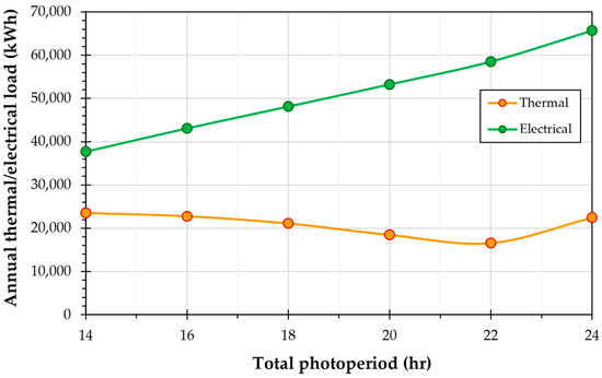
Figure 17.
Variation in annual thermal and electrical loads of the agrotunnel vs. change in the total photoperiod.
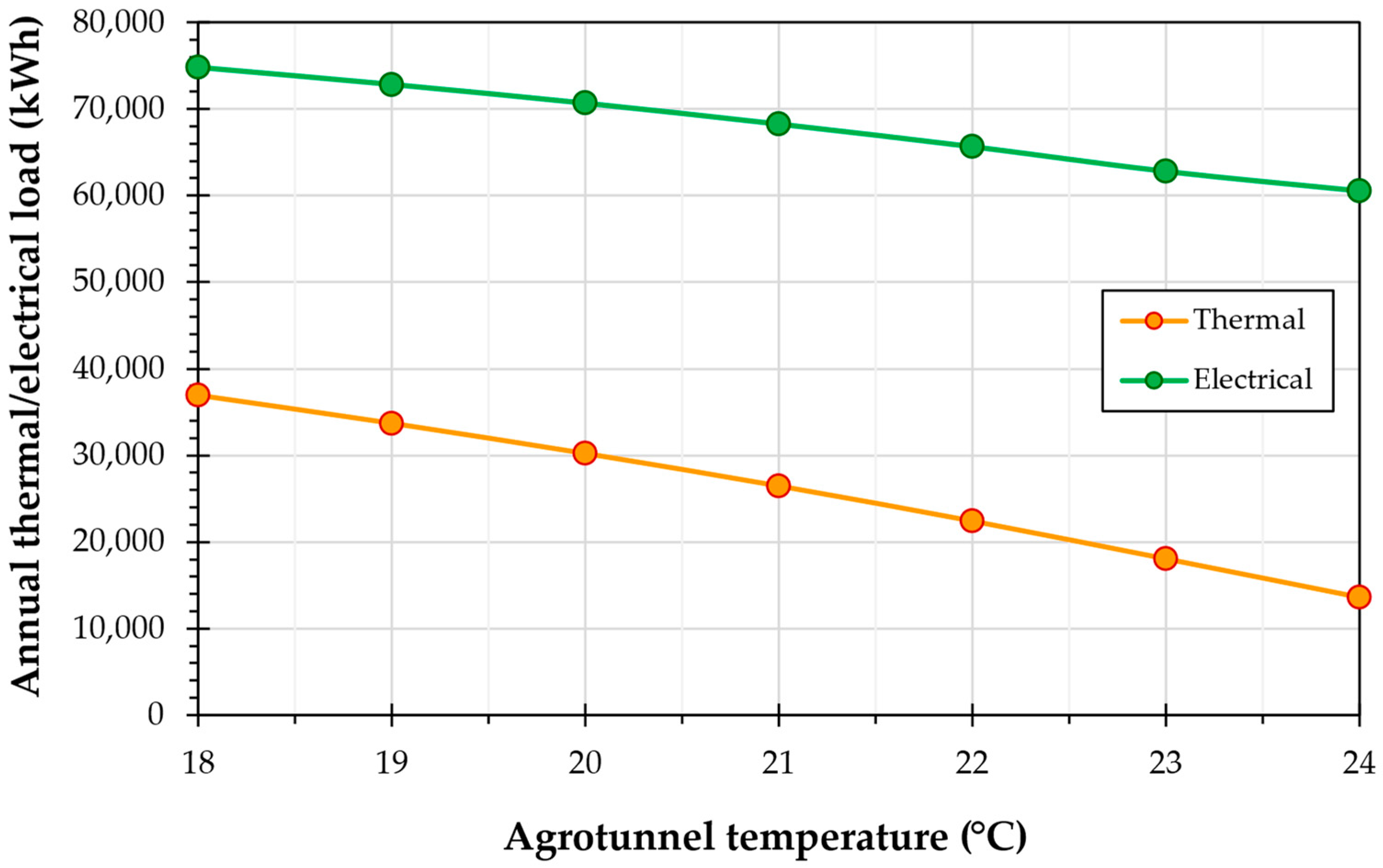
In Figure 18, it is evident that increasing the design temperature of the agrotunnel from 18 to 24 °C leads to a notable decrease in the building’s annual thermal loads, dropping from 36,942 to 13,573 kWh. This reduction primarily stems from decreased cooling demands. Consequently, the annual electrical load is expected to decrease from 74,811 to 67,943 kWh due to a drop in the electrical load of HP and dehumidifier. Notably, the design temperature emerges as a crucial parameter, significantly influencing both the thermal (with a sensitivity of 63.26%) and electrical (with a sensitivity of 19.05%) loads of the agrotunnel.
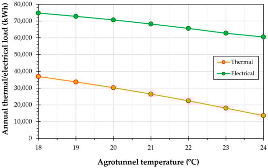
Figure 18.
Variation in annual thermal and electrical loads of the agrotunnel vs. change in the agrotunnel’s design temperature.
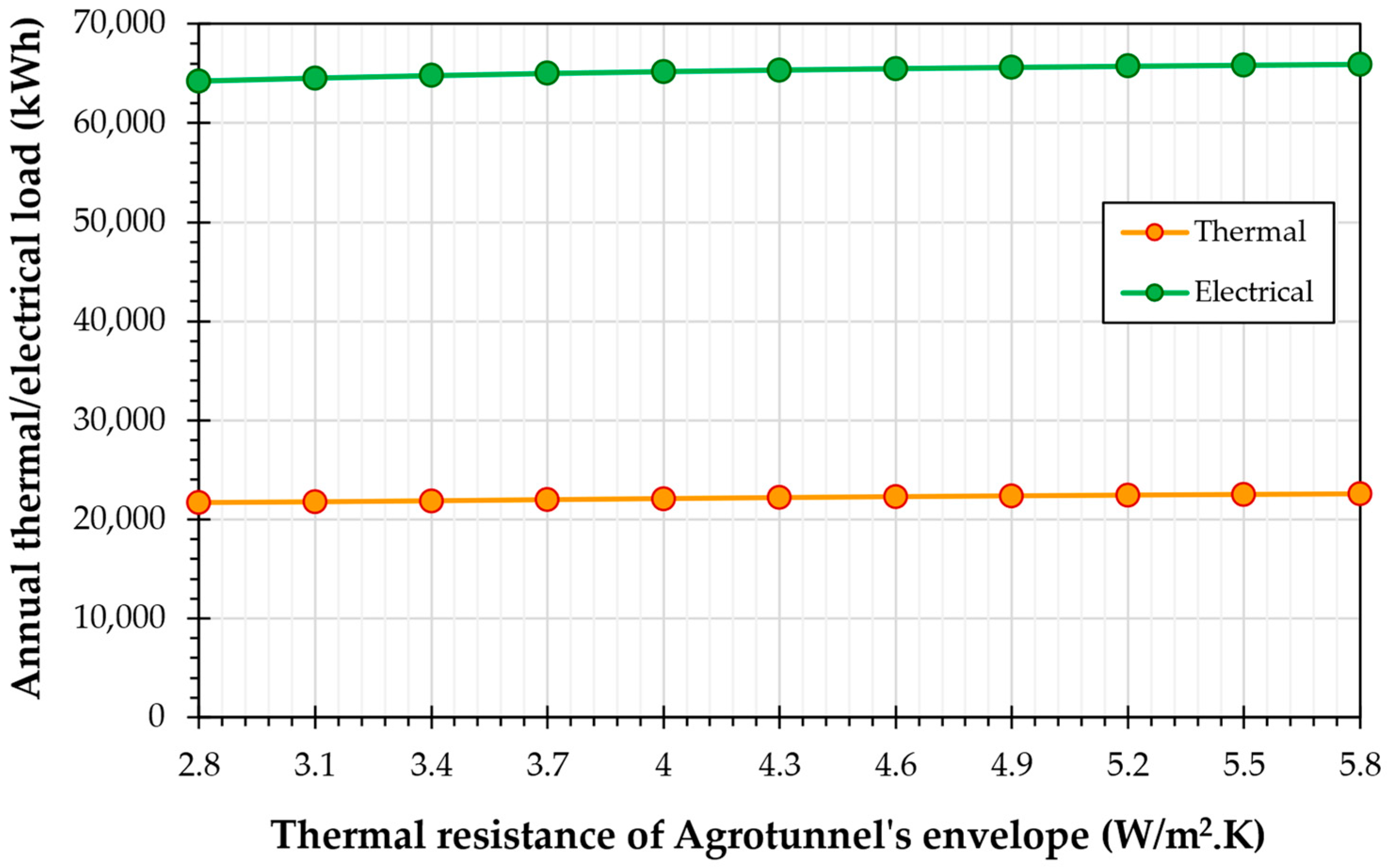
The impact of the building’s thermal resistance is investigated, with findings outlined in Figure 19. Analysis reveals that variations in the thermal resistance of the agrotunnel’s walls, ranging from 2.8 to 5.8 W/m2·K, do not yield significant changes in the thermal and electrical loads of the building. This observation suggests that factors such as lighting, evapotranspiration, and infiltration, as demonstrated in Figure 12, primarily dictate the thermal/electrical loads. Consequently, the thermal resistance parameter is not included among the influential variables.
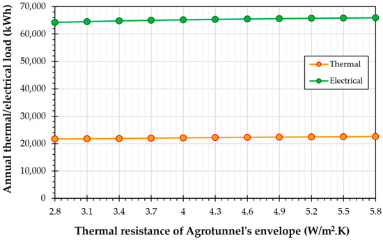
Figure 19.
Variation in annual thermal and electrical loads of the agrotunnel vs. change in the thermal resistance of the agrotunnel’s envelope.
4.4. PV System Sizing
The annual electrical energy requirements of the agrotunnel for the six locations are given in Table 10. According to Table 10, colder regions have lower energy requirements compared to warmer regions. This is because the excess heat generated by lights compensates for the heating needs imposed by the outdoor environment.
Table 10.
Annual electrical energy requirements for the agrotunnel.
The SAM results including the PV system size and the annual electrical energy generation for the six locations are detailed in Table 11.
Table 11.
PV system size for the agrotunnel.
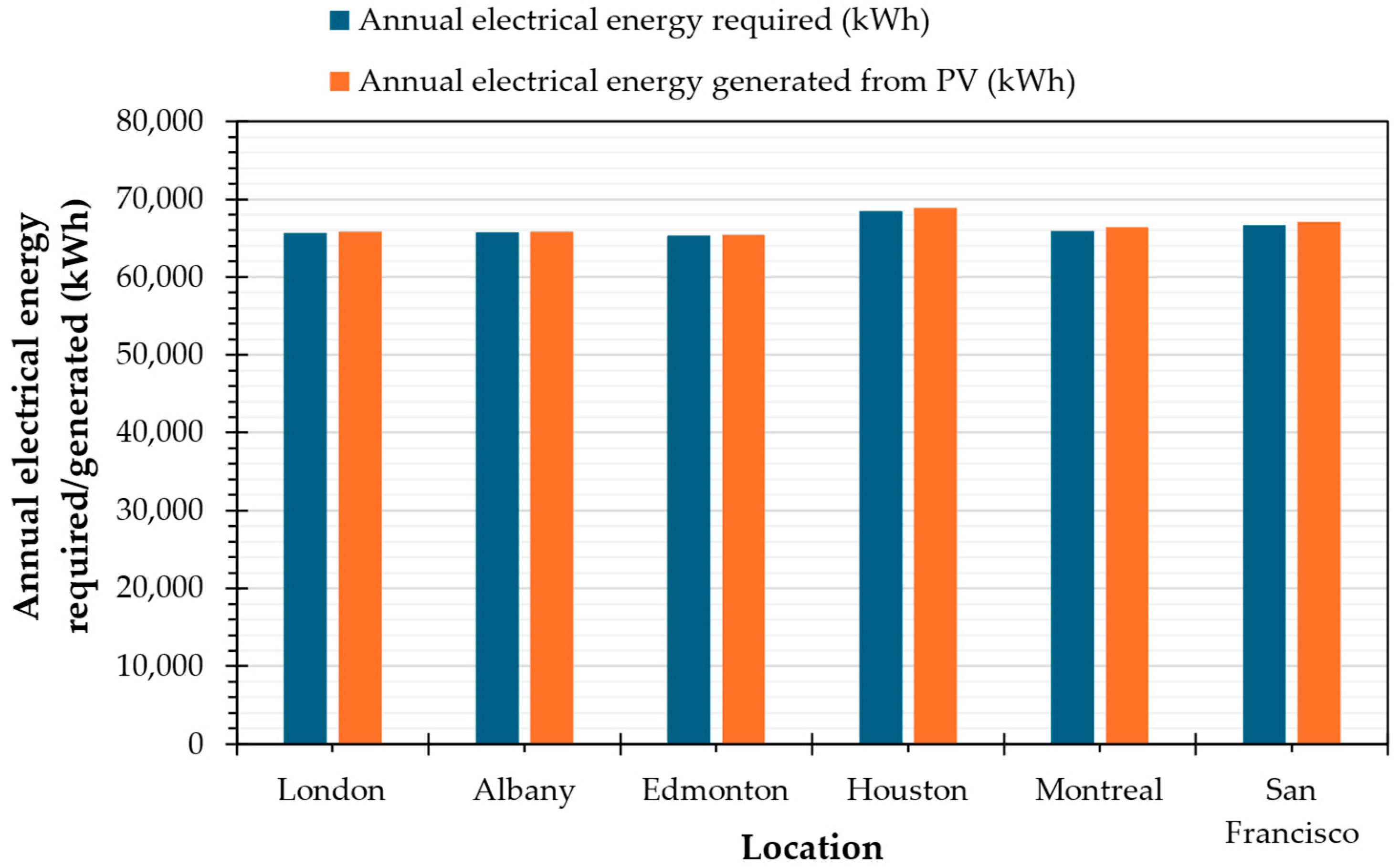
The bar graph in Figure 20 depicts the annual electrical energy required and produced by the associated PV systems for all the six locations. The chart clearly indicates that the net-zero approach has been achieved for all locations. The similar sizes of PV systems confirm that the agrotunnel’s performance is not sensitive to its location, particularly in northern climates. The smallest PV system size is needed in San Francisco (41.42 kW). Interestingly, the annual electrical output from the system in San Francisco comes out to be higher than London, Montreal, Edmonton and Albany since the electrical energy generation potential is higher in San Francisco (1641.5 kWh/kW) due to the higher level of solar irradiation there.
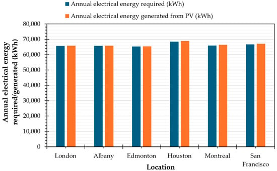
Figure 20.
Annual electrical energy required and generated for all the six locations.
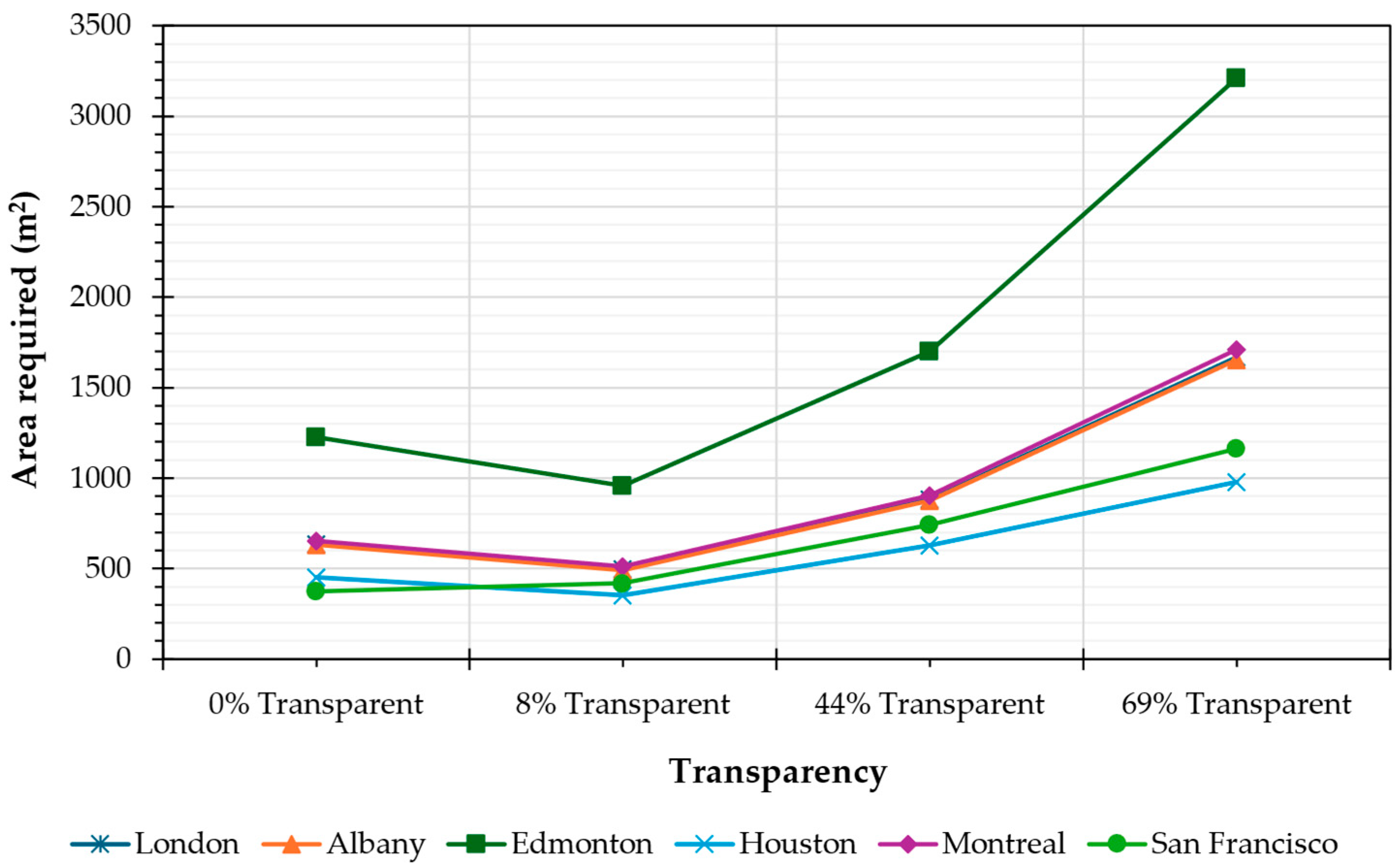
Figure 21 illustrates how the total land area used for PV installations changes with increasing module transparency. The data obtained from SAM for all locations are detailed in Table 12. A notable point in Figure 21 concerns the land required for PV system installations in Edmonton. Due to the high interrow spacing necessary to avoid shading, the total land area used for the PV system in Edmonton is considerably larger compared to other locations.
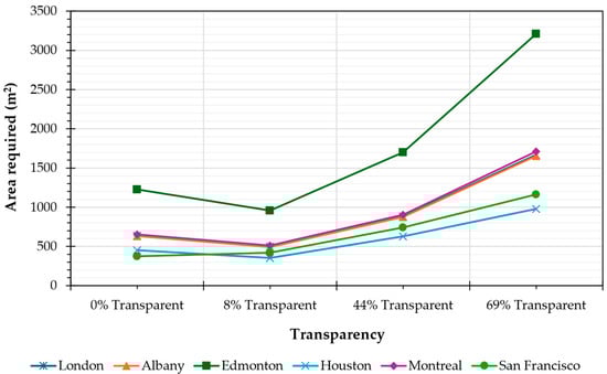
Figure 21.
Variations of land area required for PV systems with respect to the variations in the transparency of PV modules.
Table 12.
Total land area required for PV system installations.
Table 13 presents the SC and SS values for the six locations under study. Despite the higher electrical energy demand in warmer regions, such as Houston, the PV system capacity required to supply the agrotunnel is smaller. This results in higher SC and SS values due to the adequate solar irradiation levels. Among the cold regions, London, ON, Canada exhibits the highest SC and SS values.
Table 13.
Self-Consumption and Self-Sufficiency values for different locations.
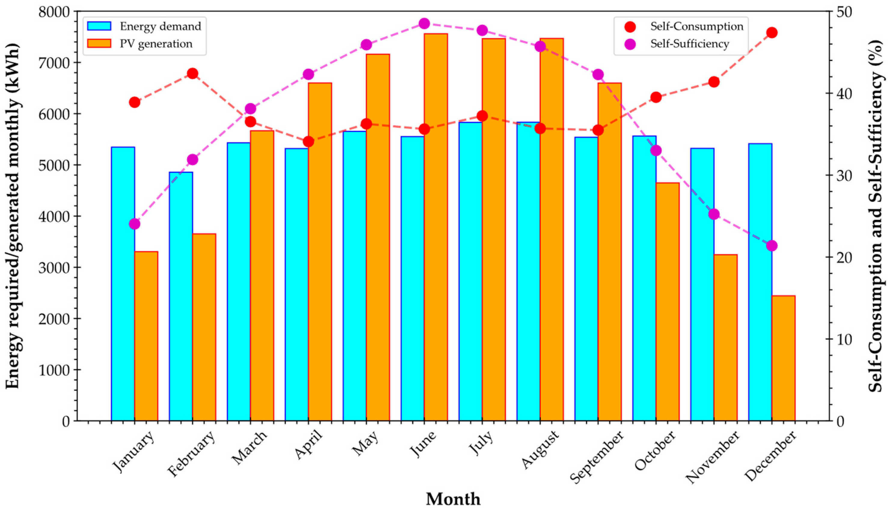
Figure 22 illustrates the monthly variations in SC and SS values over 12 months in London, ON, Canada. Figure 22 shows that SC and SS values exhibit opposite behaviors: SC increases when the electrical load exceeds the generation capacity of the PV system (e.g., in winter), whereas SS rises when the electrical demand is below the PV system’s total energy capacity (e.g., in summer).

Figure 22.
Monthly variations of self-consumption and self-sufficiency of PV system designed for London, ON, Canada.
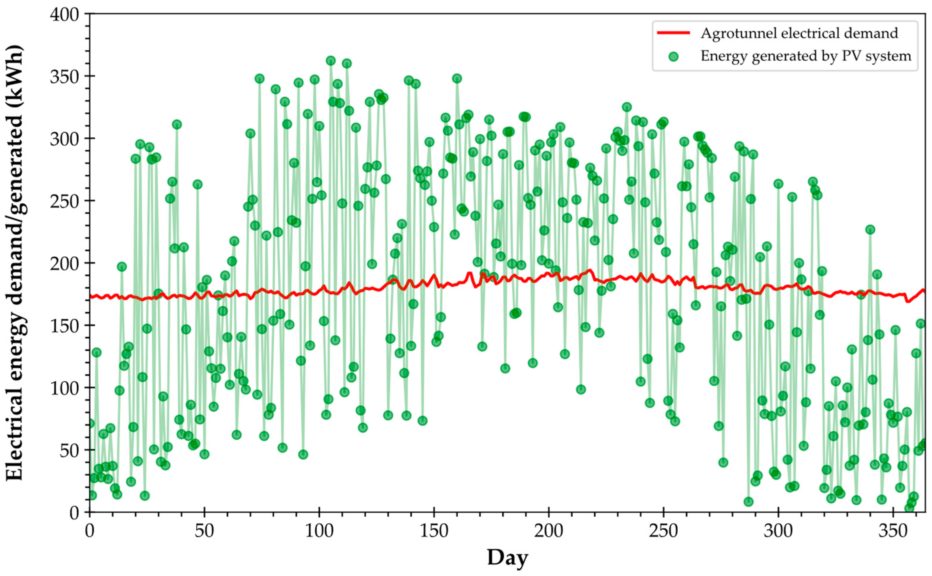
Figure 23 demonstrates that the electrical energy demand of the agrotunnel remains relatively consistent throughout the year, while the energy generated by the PV system fluctuates with variations in solar irradiation. To improve the compatibility between the load and the generated energy, and thereby increase the SS of the system, the use of electrical or thermal batteries can be considered.
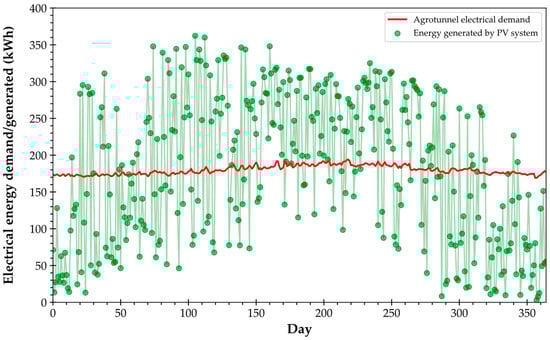
Figure 23.
Variations of daily electrical energy demand and daily energy generated by PV system over a year in London, ON, Canada.
5. Discussion
This study provides valuable insights into the feasibility of agrivoltaic agrotunnels. The PV sizes, ranging from 41.42 to 48.32 kW across locations with significantly different climates, indicate that the agrotunnel is not highly sensitive to location and climatic conditions. For conventional opaque PV modules, the required installation land area is 373 m2 in San Francisco, 453 m2 in Houston, 631 m2 in Albany, 637 m2 in London, 654 m2 in Montreal, and 1226 m2 in Edmonton. For an agrotunnel with a total surface area of 117 m2, the PV land index (total land area required by PV system to the total surface area of agrotunnel) is as follows: 3.2 m2/m2 for San Francisco, 3.87 m2/m2 for Houston, 5.39 m2/m2 for Albany, 5.44 m2/m2 for London, 5.59 m2/m2 for Montreal, and 10.48 m2/m2 for Edmonton. The solar flux level, commercial availability of PV moules and the interrow spacing alter the values for each location. The land requirements increase for systems with semi-transparent modules with transparencies of 8, 44, and 69%.
By utilizing single-axis tracking PV systems on just 1% of the total agricultural lands in Ontario, Quebec, and Alberta [86], it is possible to power more than 231, 220, and 534 thousands of agrotunnels in these regions, respectively. This demonstrates the potential of this technology to enhance food security, especially in areas with harsh climates where local food production is challenging and energy, operation, and transportation costs are high [87]. In grid-tied conventional formats, the high capital costs of indoor farming facilities and the vertical farming industry [88] have deterred many investors [89], leading to farm closures, asset sales, loan defaults, and company bankruptcies [90,91,92,93,94,95,96,97,98,99]. Some industry giants, operating multiple industrial-scale farms with significant funding, have gone bankrupt after 20 years [100], and many startups have failed due to high operational costs and lower-than-expected crop yields [100,101]. In this context, becoming less dependent on the electricity grid by using affordable renewable energy sources, such as PV technology, can help many companies survive. For this, an open-source thermal–electrical model has been developed in the current study for predicting the energy demands of a semi-commercial scale indoor vertical farming facility, the agrotunnel. The model has been validated using commercial software, industrial datasheets, and real-time data from the agrotunnel, making it reliable and applicable to various locations. Investors and farmers can use this model and the findings of this research to evaluate the energy requirements of indoor farming, thereby investing in such technologies with greater confidence. With the PV systems sized appropriately as shown here, agrivoltaics agrotunnel investors are completely insulated from electricity price fluctuations. Similarly, when compared to competitors that use natural gas for heating, the agrivoltaics agrotunnel economics are not impacted by natural gas fluctuations. An upfront cost in solar PV means that all operational energy for 25 years on the agrivoltaics agrotunnel is known and paid for via financing.
The open-source model provided in this study is available for researchers worldwide to assess, modify, and upgrade to address its limitations. Currently, the model only considers the plug loads in the agrotunnel. Safety factors must be incorporated for future potential loads. Moreover, the loads have been modeled based on assumptions regarding the types and ages of the crops. For more accurate energy predictions, a dynamic model can be developed that accounts for the plants’ growth over time. The heat pump model can be enhanced from a black-box model to a thermodynamic model, increasing compatibility with various conditions and environmental limitations. Additionally, a comprehensive economic model should be developed to compare capital, labor, and energy costs. Future economic investigations will offer more valuable insights for farmers and investors. This study focused on ensuring net zero energy grid tied systems. Ultimately, the feasibility of off-grid PV systems, capable of covering the electricity loads of the agrotunnel by 100% self-consumption, along with the necessary battery capacity sizing, can be assessed in future studies.
6. Conclusions
This study developed and validated a thermal–electrical model to size a net-zero agrivoltaics array for an indoor-growing agrotunnel. It incorporated wall transmission, infiltrations, and plant evapotranspiration effects in the thermal model, and heat pump sizing for temperature control, as well as using the measured plug loads such as those of water pumps, LED lighting, and dehumidifiers. Thermal analysis showed that in an agrotunnel in London, ON, Canada lights contributed 40% of the thermal load, while plant evapotranspiration added 32%. Sensible infiltration and wall transmission together accounted for about 25% of the thermal load, while the presence of people had a negligible impact on the thermal load.
The choice of crop in an agrotunnel could significantly impact the water usage and building load due to varying evapotranspiration rates of some crops. Although the thermal load remained consistent since the evapotranspiration is an isenthalpic process, power demand decreased as dehumidifier’s electricity consumption dropped as a result of reduced latent load. For example, growing kale, which requires frequent watering, increased annual electricity demand by 25.53% compared to herbs (basil, parsley, oregano, and rosemary), and by 32.26 and 34.32% compared to vegetables and fruits (tomatoes, beans, and strawberries) and lettuce, respectively.
Reducing the photoperiod from 24 to 14 h per day significantly decreased the annual electrical load of an agrotunnel from 65,658 to 37,711 kWh, primarily due to reduced lighting power. In colder climates, extended photoperiods helped offset heating demands due to lights’ dissipated energy. Hence, optimizing photoperiods is crucial, especially when conventional non-electrical sources supply thermal demands.
The design temperature was a crucial parameter, strongly influencing both thermal (63.26% sensitivity) and electrical (19.05% sensitivity) loads.
The agrotunnels located in colder regions have lower annual electrical energy requirements compared to those in warmer regions. In colder regions, the excess heat generated by the lights offsets the heating needs caused by the outdoor environment.
According to the PV sizing results, the net-zero target was achieved for the annual electrical energy requirements and production from PV systems across six locations (London, Montreal, Edmonton, Albany, San Francisco, and Houston). Albany required the largest PV capacity at 48.32 kW to meet its annual energy demand of 67,497 kWh. Conversely, San Francisco needed the smallest system size at 41.42 kW. The PV system capacity for an agrotunnel in warmer regions such as Houston was smaller due to ample solar irradiation. Consequently, these regions showed higher Self-Consumption (SC) and Self-Sufficiency (SS) values.
London, ON, among the colder regions, exhibited the highest SC and SS values overall. Additionally, evaluating the monthly trend of SC and SS values proved that they behave oppositely: SC increased during months when electrical demand surpassed PV system generation capacity (e.g., winter), while SS rose when demand fell below the PV system’s energy capacity (e.g., summer).
Author Contributions
Conceptualization, J.M.P.; methodology, N.A., U.J. and J.M.P.; software, N.A. and U.J.; validation, N.A., U.J. and J.M.P.; formal analysis, N.A., U.J. and J.M.P.; investigation, N.A. and U.J.; resources, J.M.P.; data curation, N.A. and U.J.; writing—original draft preparation, N.A., U.J. and J.M.P.; writing—review and editing, N.A., U.J. and J.M.P.; visualization, N.A. and U.J.; supervision, J.M.P.; project administration, J.M.P.; funding acquisition, J.M.P. All authors have read and agreed to the published version of the manuscript.
Funding
This work was supported by the Weston Family Foundation through the Homegrown Challenge, Carbon Solutions @ Western and the Thompson Endowment.
Institutional Review Board Statement
Not applicable.
Informed Consent Statement
Not applicable.
Data Availability Statement
Data for this manuscript is available at: https://osf.io/sdt74/files/osfstorage (accessed on 11 July 2024).
Acknowledgments
The authors would like to thank Greg Whiteside and Jeremy Van Maar for helpful discussion and technical assistance.
Conflicts of Interest
The authors declare no conflicts of interest.
References
- US EPA Organization. Global Greenhouse Gas Overview. Available online: https://www.epa.gov/ghgemissions/global-greenhouse-gas-overview (accessed on 19 June 2024).
- Beacham, A.M.; Vickers, L.H.; Monaghan, J.M. Vertical Farming: A Summary of Approaches to Growing Skywards. J. Hortic. Sci. Biotechnol. 2019, 94, 277–283. [Google Scholar] [CrossRef]
- Ampim, P.A.Y.; Obeng, E.; Olvera-Gonzalez, E. Indoor Vegetable Production: An Alternative Approach to Increasing Cultivation. Plants 2022, 11, 2843. Available online: https://www.mdpi.com/2223-7747/11/21/2843 (accessed on 19 June 2024). [CrossRef]
- Sadek, N.; Kamal, N.; Shehata, D. Internet of Things Based Smart Automated Indoor Hydroponics and Aeroponics Greenhouse in Egypt. Ain Shams Eng. J. 2024, 15, 102341. [Google Scholar] [CrossRef]
- Stein, E.W. The Transformative Environmental Effects Large-Scale Indoor Farming May Have on Air, Water, and Soil. Air Soil Water Res. 2021, 14. Available online: https://journals.sagepub.com/doi/full/10.1177/1178622121995819 (accessed on 19 June 2024). [CrossRef]
- Mitchell, C.A. History of Controlled Environment Horticulture: Indoor Farming and Its Key Technologies. HortScience 2022, 57, 247–256. [Google Scholar] [CrossRef]
- Ahamed, M.S.; Sultan, M.; Monfet, D.; Rahman, M.S.; Zhang, Y.; Zahid, A.; Bilal, M.; Ahsan, T.M.A.; Achour, Y. A Critical Review on Efficient Thermal Environment Controls in Indoor Vertical Farming. J. Clean. Prod. 2023, 425, 138923. [Google Scholar] [CrossRef]
- Sheibani, F.; Bourget, M.; Morrow, R.C.; Mitchell, C.A. Close-Canopy Lighting, an Effective Energy-Saving Strategy for Overhead Sole-Source LED Lighting in Indoor Farming. Front. Plant Sci. 2023, 14, 1215919. [Google Scholar] [CrossRef]
- Hachem-Vermette, C.; MacGregor, A. Energy Optimized Envelope for Cold Climate Indoor Agricultural Growing Center. Buildings 2017, 7, 59. [Google Scholar] [CrossRef]
- Avgoustaki, D.D.; Xydis, G. Indoor Vertical Farming in the Urban Nexus Context: Business Growth and Resource Savings. Sustainability 2020, 12, 1965. [Google Scholar] [CrossRef]
- Despommier, D. Vertical Farms, Building a Viable Indoor Farming Model for Cities. Field Actions Science Reports. J. Field Actions 2019, 14, 68–73. [Google Scholar]
- George, P.; George, N. Hydroponics-(Soilless Cultivation of Plants) for Biodiversity Conservation. Int. J. Mod. Trends Eng. Sci 2016, 3, 97–104. [Google Scholar]
- Pinstrup-Andersen, P. Is It Time to Take Vertical Indoor Farming Seriously? Glob. Food Secur. 2018, 17, 233–235. [Google Scholar] [CrossRef]
- Walling, M. As Indoor Farming Startups with Hundreds of Millions in Funding Head to Bankruptcy, Critic Says: “Boy, This Is a Dumb Idea”. Available online: https://fortune.com/2023/09/18/indoor-farming-startups-bankruptcy-dumb-idea-expensive/ (accessed on 29 March 2024).
- Vandewetering, N.; Hayibo, K.S.; Pearce, J.M. Open-Source Design and Economics of Manual Variable-Tilt Angle DIY Wood-Based Solar Photovoltaic Racking System. Designs 2022, 6, 54. [Google Scholar] [CrossRef]
- Riaz, M.H.; Imran, H.; Butt, N.Z. Optimization of PV Array Density for Fixed Tilt Bifacial Solar Panels for Efficient Agrivoltaic Systems. In Proceedings of the 2020 47th IEEE Photovoltaic Specialists Conference (PVSC), Calgary, AL, Canada, 15 June–21 August 2020; pp. 1349–1352. [Google Scholar]
- Tahir, Z.; Butt, N.Z. Implications of Spatial-Temporal Shading in Agrivoltaics under Fixed Tilt & Tracking Bifacial Photovoltaic Panels. Renew. Energy 2022, 190, 167–176. [Google Scholar] [CrossRef]
- Jamil, U.; Vandewetering, N.; Sadat, S.A.; Pearce, J.M. Wood- and Cable-Based Variable Tilt Stilt-Mounted Solar Photovoltaic Racking System. Designs 2024, 8, 6. [Google Scholar] [CrossRef]
- Krexner, T.; Bauer, A.; Gronauer, A.; Mikovits, C.; Schmidt, J.; Kral, I. Environmental Life Cycle Assessment of a Stilted and Vertical Bifacial Crop-Based Agrivoltaic Multi Land-Use System and Comparison with a Mono Land-Use of Agricultural Land. Renew. Sustain. Energy Rev. 2024, 196, 114321. [Google Scholar] [CrossRef]
- Jamil, U.; Vandewetering, N.; Pearce, J.M. Solar Photovoltaic Wood Racking Mechanical Design for Trellis-Based Agrivoltaics. PLoS ONE 2023, 18, e0294682. [Google Scholar] [CrossRef] [PubMed]
- Malu, P.R.; Sharma, U.S.; Pearce, J.M. Agrivoltaic Potential on Grape Farms in India. Sustain. Energy Technol. Assess. 2017, 23, 104–110. [Google Scholar] [CrossRef]
- Padilla, J.; Toledo, C.; Abad, J. Enovoltaics: Symbiotic Integration of Photovoltaics in Vineyards. Front. Energy Res. 2022, 10, 1007383. [Google Scholar] [CrossRef]
- Hayibo, K.S.; Pearce, J.M. Optimal Inverter and Wire Selection for Solar Photovoltaic Fencing Applications. Renew. Energy Focus 2022, 42, 115–128. [Google Scholar] [CrossRef]
- Masna, S.; Morse, S.M.; Hayibo, K.S.; Pearce, J.M. The Potential for Fencing to Be Used as Low-Cost Solar Photovoltaic Racking. Sol. Energy 2023, 253, 30–46. [Google Scholar] [CrossRef]
- Hwang, K.-W.; Lee, C.-Y. Estimating the Deterministic and Stochastic Levelized Cost of the Energy of Fence-Type Agrivoltaics. Energies 2024, 17, 1932. [Google Scholar] [CrossRef]
- Imran, H.; Riaz, M.H.; Butt, N.Z. Optimization of Single-Axis Tracking of Photovoltaic Modules for Agrivoltaic Systems. In Proceedings of the 2020 47th IEEE Photovoltaic Specialists Conference (PVSC), Calgary, AL, Canada, 15 June–21 August 2020; pp. 1353–1356. [Google Scholar]
- Casares de la Torre, F.J.; Varo, M.; López-Luque, R.; Ramírez-Faz, J.; Fernández-Ahumada, L.M. Design and Analysis of a Tracking/Backtracking Strategy for PV Plants with Horizontal Trackers after Their Conversion to Agrivoltaic Plants. Renew. Energy 2022, 187, 537–550. [Google Scholar] [CrossRef]
- Campana, P.E.; Stridh, B.; Amaducci, S.; Colauzzi, M. Optimisation of Vertically Mounted Agrivoltaic Systems. J. Clean. Prod. 2021, 325, 129091. [Google Scholar] [CrossRef]
- Jamil, U.; Bonnington, A.; Pearce, J.M. The Agrivoltaic Potential of Canada. Sustainability 2023, 15, 3228. [Google Scholar] [CrossRef]
- Riaz, M.H.; Imran, H.; Younas, R.; Butt, N.Z. The Optimization of Vertical Bifacial Photovoltaic Farms for Efficient Agrivoltaic Systems. Sol. Energy 2021, 230, 1004–1012. [Google Scholar] [CrossRef]
- Hayibo, K.S.; Pearce, J.M. Vertical Free-Swinging Photovoltaic Racking Energy Modeling: A Novel Approach to Agrivoltaics. Renew. Energy 2023, 218, 119343. [Google Scholar] [CrossRef]
- Vandewetering, N.; Hayibo, K.S.; Pearce, J.M. Open-Source Vertical Swinging Wood-Based Solar Photovoltaic Racking Systems. Designs 2023, 7, 34. [Google Scholar] [CrossRef]
- Fu, R.; Feldman, D.J.; Margolis, R.M. US Solar Photovoltaic System Cost Benchmark: Q1 2018; NREL: Golden, CO, USA, 2018.
- Walker, M. Solar Panel Cost: Avg. Solar Panel Cost in 2024, EnergySage. Solar News. 2024. Available online: https://www.energysage.com/local-data/solar-panel-cost/ (accessed on 17 June 2024).
- Dudley, D. Renewable Energy Will Be Consistently Cheaper than Fossil Fuels By 2020; Forbes: Jersey City, NJ, USA, 2019. [Google Scholar]
- Solar Industry Research Data|SEIA. Available online: https://www.seia.org/solar-industry-research-data (accessed on 2 January 2024).
- Saefong, M.P. Why Solar Is the Fastest-Growing Source of U.S. Electricity–MarketWatch. Available online: https://www.marketwatch.com/story/why-solar-is-the-fastest-growing-source-of-u-s-electricity-72e7d489 (accessed on 17 June 2024).
- Vaughan, A. Time to Shine: Solar Power Is Fastest-Growing Source of New Energy. The Guardian, 4 October 2017. [Google Scholar]
- Barbose, G.L.; Darghouth, N.R.; LaCommare, K.H.; Millstein, D.; Rand, J. Tracking the Sun: Installed Price Trends for Distributed Photovoltaic Systems in the United States—2018, 2018 ed.; Lawrence Berkeley National Laboratory: Berkeley, CA, USA, 2018.
- Calvert, K.; Mabee, W. More Solar Farms or More Bioenergy Crops? Mapping and Assessing Potential Land-Use Conflicts among Renewable Energy Technologies in Eastern Ontario, Canada. Appl. Geogr. 2015, 56, 209–221. [Google Scholar] [CrossRef]
- Calvert, K.; Pearce, J.M.; Mabee, W.E. Toward Renewable Energy Geo-Information Infrastructures: Applications of GIScience and Remote Sensing That Build Institutional Capacity. Renew. Sustain. Energy Rev. 2013, 18, 416–429. [Google Scholar] [CrossRef]
- Sovacool, B.K. Exploring and Contextualizing Public Opposition to Renewable Electricity in the United States. Sustainability 2009, 1, 702–721. [Google Scholar] [CrossRef]
- Sovacool, B.K.; Lakshmi Ratan, P. Conceptualizing the Acceptance of Wind and Solar Electricity. Renew. Sustain. Energy Rev. 2012, 16, 5268–5279. [Google Scholar] [CrossRef]
- Pearce, J.M. Agrivoltaics in Ontario Canada: Promise and Policy. Sustainability 2022, 14, 3037. [Google Scholar] [CrossRef]
- Dupraz, C.; Marrou, H.; Talbot, G.; Dufour, L.; Nogier, A.; Ferard, Y. Combining Solar Photovoltaic Panels and Food Crops for Optimising Land Use: Towards New Agrivoltaic Schemes. Renew. Energy 2011, 36, 2725–2732. [Google Scholar] [CrossRef]
- Guerin, T.F. Impacts and Opportunities from Large-Scale Solar Photovoltaic (PV) Electricity Generation on Agricultural Production. Environ. Qual. Manag. 2019, 28, 7–14. [Google Scholar] [CrossRef]
- Valle, B.; Simonneau, T.; Sourd, F.; Pechier, P.; Hamard, P.; Frisson, T.; Ryckewaert, M.; Christophe, A. Increasing the Total Productivity of a Land by Combining Mobile Photovoltaic Panels and Food Crops. Appl. Energy 2017, 206, 1495–1507. [Google Scholar] [CrossRef]
- Mavani, D.D.; Chauhan, P.M.; Joshi, V. Beauty of Agrivoltaic System Regarding Double Utilization of Same Piece of Land for Generation of Electricity & Food Production. Int. J. Sci. Eng. Res. 2019, 10, 118–148. [Google Scholar]
- Trommsdorff, M.; Kang, J.; Reise, C.; Schindele, S.; Bopp, G.; Ehmann, A.; Weselek, A.; Högy, P.; Obergfell, T. Combining Food and Energy Production: Design of an Agrivoltaic System Applied in Arable and Vegetable Farming in Germany. Renew. Sustain. Energy Rev. 2021, 140, 110694. [Google Scholar] [CrossRef]
- Mow, B. Solar Sheep and Voltaic Veggies: Uniting Solar Power and Agriculture. Available online: https://www.nrel.gov/state-local-tribal/blog/posts/solar-sheep-and-voltaic-veggies-uniting-solar-power-and-agriculture.html (accessed on 1 April 2023).
- Nassar, A.; Perez-Wulf, I.; Hameiri, Z. Improving Productivity of Cropland through Agrivoltaics; APVI: Sydney, Australia, 2020. [Google Scholar]
- Amaducci, S.; Yin, X.; Colauzzi, M. Agrivoltaic Systems to Optimise Land Use for Electric Energy Production. Appl. Energy 2018, 220, 545–561. [Google Scholar] [CrossRef]
- Reasoner, M.; Ghosh, A. Agrivoltaic Engineering and Layout Optimization Approaches in the Transition to Renewable Energy Technologies: A Review. Challenges 2022, 13, 43. [Google Scholar] [CrossRef]
- Kumpanalaisatit, M.; Setthapun, W.; Sintuya, H.; Pattiya, A.; Jansri, S.N. Current Status of Agrivoltaic Systems and Their Benefits to Energy, Food, Environment, Economy, and Society. Sustain. Prod. Consum. 2022, 33, 952–963. [Google Scholar] [CrossRef]
- Giri, N.C.; Mohanty, R.C. Agrivoltaic System: Experimental Analysis for Enhancing Land Productivity and Revenue of Farmers. Energy Sustain. Dev. 2022, 70, 54–61. [Google Scholar] [CrossRef]
- Food Security Structures Canada. Available online: https://www.foodsecuritystructures.ca/home (accessed on 25 March 2024).
- Food Security Structures Canada—Better Grow Lights. Available online: https://www.foodsecuritystructures.ca/growing-systems/better-grow-lights (accessed on 29 February 2024).
- Bhatia, A. Cooling Load Calculations and Principles; Continuing Education and Development, Inc.: Stony Point, NY, USA, 2001; p. 39. [Google Scholar]
- ASHRAE. ASHRAE Fundamentals Handbook; ASHRAE: Peachtree Corners, GA, USA, 1997. [Google Scholar]
- Cengel, Y.A. Heat Transfer: A Practical Approach; McGraw-Hill: New York, NY, USA, 1998. [Google Scholar]
- McQuiston, F.C.; Parker, J.D.; Spitler, J.D.; Taherian, H. Heating, Ventilating, and Air Conditioning: Analysis and Design; John Wiley & Sons: Hoboken, NJ, USA, 2023; ISBN 1-119-89416-6. [Google Scholar]
- Asgari, N.; McDonald, M.T.; Pearce, J.M. Energy Modeling and Techno-Economic Feasibility Analysis of Greenhouses for Tomato Cultivation Utilizing the Waste Heat of Cryptocurrency Miners. Energies 2023, 16, 1331. [Google Scholar] [CrossRef]
- Kumar, R.; Shankar, V.; Kumar, M. Modelling of Crop Reference Evapotranspiration: A Review. Univers. J. Environ. Res. Technol. 2011, 1, 239–242. [Google Scholar]
- Subedi, A.; Chávez, J.L. Crop Evapotranspiration (ET) Estimation Models: A Review and Discussion of the Applicability and Limitations of ET Methods. J. Agric. Sci. 2015, 7, p50. [Google Scholar] [CrossRef]
- Midwest Machinery. How to Size an HVAC for Maximum Grow Margin. Available online: https://midwestmachinery.net/wp-content/uploads/2020/01/Ultimate-Grow-Room-HVAC-Guide.pdf (accessed on 11 July 2024).
- Heat Pump | GSZ16 | Up to 16 SEER | 9.0 HSPF | Goodman. Available online: https://www.goodmanmfg.com/products/heat-pumps/16-seer-gsz16 (accessed on 25 March 2024).
- Li, S.; Gong, G.; Peng, J. Dynamic Coupling Method between Air-Source Heat Pumps and Buildings in China’s Hot-Summer/Cold-Winter Zone. Appl. Energy 2019, 254, 113664. [Google Scholar] [CrossRef]
- Emporia Energy. Energy Vue. Available online: https://web.emporiaenergy.com/ (accessed on 3 April 2024).
- Oberloier, S.; Pearce, J.M. Open source low-cost power monitoring system. HardwareX 2018, 4, e00044. [Google Scholar] [CrossRef]
- Viciana, E.; Alcayde, A.; Montoya, F.G.; Baños, R.; Arrabal-Campos, F.M.; Zapata-Sierra, A.; Manzano-Agugliaro, F. OpenZmeter: An Efficient Low-Cost Energy Smart Meter and Power Quality Analyzer. Sustainability 2018, 10, 4038. [Google Scholar] [CrossRef]
- NOMA 50 Pint LED Dehumidifier with Pump, Bucket/Continuous Drain, ENERGY STAR® Most Efficient, White | Canadian Tire. Available online: https://www.canadiantire.ca/en/pdp/noma-50-pint-led-dehumidifier-with-pump-bucket-continuous-drain-energy-star-most-efficient-white-0430755p.html (accessed on 27 March 2024).
- Rule of Thumb Calculations (400 Cfm/Ton). Available online: https://tranecds.custhelp.com/app/answers/detail/a_id/918/~/rule-of-thumb-calculations-%28400-cfm%2Fton%29 (accessed on 2 April 2024).
- Beekist Growers. Available online: https://www.facebook.com/p/Beekist-Growers-61551502111382/ (accessed on 9 July 2024).
- National Renewable Energy Laboratory SAM Open Source—System Advisor Model—SAM. Available online: https://sam.nrel.gov/sam-open-source.html (accessed on 15 December 2022).
- Ciocia, A.; Amato, A.; Di Leo, P.; Fichera, S.; Malgaroli, G.; Spertino, F.; Tzanova, S. Self-Consumption and Self-Sufficiency in Photovoltaic Systems: Effect of Grid Limitation and Storage Installation. Energies 2021, 14, 1591. [Google Scholar] [CrossRef]
- Asgari, N.; Hayibo, K.S.; Groza, J.; Rana, S.; Pearce, J.M. Greenhouse Applications of Solar Photovoltaic Driven Heat Pumps in Northern Environments; Western University: London, ON, Canada, 2024; to be published. [Google Scholar]
- Rana, S.; Jamil, U.; Asgari, N.; Hayibo, K.S.; Groza, J.; Pearce, J.M. Residential Sizing of Solar Photovoltaic Systems and Heat Pumps for Net Zero Sustainable Thermal Building Energy. Computation 2024, 12, 126. [Google Scholar] [CrossRef]
- Available online: https://heliene.com/144hc-m6-bifacial-module/ (accessed on 11 July 2024).
- Solar Power Calculator Ontario, Canada. Available online: https://solarcalculator.ca/province/Ontario/ (accessed on 22 June 2024).
- Alberta, S. Winter Effects on Solar PV Efficiency. Available online: https://solaralberta.ca/members/business-member-resources/alberta-solar-performance-data/ (accessed on 22 June 2024).
- Robinson, A. Solar PV Analysis of Houston, United States. Available online: https://profilesolar.com/locations/United-States/Houston/ (accessed on 22 June 2024).
- Available online: https://quebecsolar.ca/solar-energy-facts-quebec-solar-installation-company-montreal/ (accessed on 11 July 2024).
- Solar Panel Angles for San Francisco, California, US. Available online: https://solarific.co (accessed on 22 June 2024).
- London International Airport | Weather History & Climate. Available online: https://meteostat.net/en/station/71623?t=2024-02-17/2024-02-24 (accessed on 13 June 2024).
- Castilla, N. Greenhouse Technology and Management; Cabi: Delémont, Switzerland, 2013; ISBN 1-78064-103-6. [Google Scholar]
- Jamil, U.; Pearce, J.M. Maximizing Biomass with Agrivoltaics: Potential and Policy in Saskatchewan Canada. Biomass 2023, 3, 188–216. [Google Scholar] [CrossRef]
- D’Souza, S.; Guerriero, L.; Ellenwood, L.; Angelovski, I. What’s Behind Rising Food Costs in Canada’s North? Questions Emerge over How Retailer Sets Prices. CBC News, 23 February 2024. [Google Scholar]
- Lessons from Vertical Farming Bankruptcies, Layoffs, and Closures in 2023. Available online: https://www.verticalfarmdaily.com/article/9537965/lessons-from-vertical-farming-bankruptcies-layoffs-and-closures-in-2023/ (accessed on 23 June 2024).
- Riemenschneider, P. Indoor Farming Operations Face Bankruptcies, Layoffs, Closures; Produce Blue Book: Carol Stream, IL, USA, 2023. [Google Scholar]
- Johnson, G. 80 Acres Farms Makes Layoffs; Produce Blue Book: Carol Stream, IL, USA, 2023. [Google Scholar]
- Riemenschneider, P. AppHarvest Opens 60-Acre Kentucky Farm, Completes $127MM Sale-Leaseback with Mastronardi Berea LLC; Produce Blue Book: Carol Stream, IL, USA, 2022. [Google Scholar]
- Riemenschneider, P. AppHarvest Opens Salad Farm Backed by $30 Million Mastonardi Produce Loan; Produce Blue Book: Carol Stream, IL, USA, 2022. [Google Scholar]
- Johnson, G. Edible Garden Approves Reverse Stock Split; Produce Blue Book: Carol Stream, IL, USA, 2023. [Google Scholar]
- Riemenschneider, P. Faced with Nasdaq Delisting, Kalera Shareholders Approve Reverse Stock Split; Produce Blue Book: Carol Stream, IL, USA, 2022. [Google Scholar]
- Riemenschneider, P. Kalera Halts Orlando, Atlanta Production to Focus on Profitability at Other Facilities; Produce Blue Book: Carol Stream, IL, USA, 2023. [Google Scholar]
- Heater, B. Iron Ox Lays off 50, Amounting to Nearly Half Its Staff. Available online: https://techcrunch.com/2022/11/03/iron-ox-lays-off-50-amounting-to-nearly-half-its-staff/ (accessed on 23 June 2024).
- Marston, J. Brief: Plenty Confirms Closure of South San Francisco Vertical Farming Facility. Available online: https://agfundernews.com/plenty-confirms-closure-of-south-san-francisco-vertical-farming-facility (accessed on 23 June 2024).
- Johnson, G. Lakeside Produce Files Bankruptcy, Owes $188MM; Produce Blue Book: Carol Stream, IL, USA, 2023. [Google Scholar]
- Vertical Farming Robotics Startup Fifth Season Shuts Down. Available online: https://www.bizjournals.com/pittsburgh/news/2022/10/29/vertical-farming-startup-fifth-season-shuts-down.html (accessed on 23 June 2024).
- Indoor Agriculture Faces a Reckoning | Ambrook Research. Available online: https://ambrook.com/research/supply-chain/vertical-farms-venture-capital-chapter-11 (accessed on 23 June 2024).
- Indoor Farming Company AppHarvest Files for Bankruptcy. Available online: https://www.agriculturedive.com/news/appharvest-bankruptcy-indoor-farming-martha-stewart-jd-vance/689039/ (accessed on 23 June 2024).


Disclaimer/Publisher’s Note: The statements, opinions and data contained in all publications are solely those of the individual author(s) and contributor(s) and not of MDPI and/or the editor(s). MDPI and/or the editor(s) disclaim responsibility for any injury to people or property resulting from any ideas, methods, instructions or products referred to in the content. |
© 2024 by the authors. Licensee MDPI, Basel, Switzerland. This article is an open access article distributed under the terms and conditions of the Creative Commons Attribution (CC BY) license (https://creativecommons.org/licenses/by/4.0/).