Spatiotemporal Analysis of Air Quality and Its Driving Factors in Beijing’s Main Urban Area

Abstract

Urban air pollution is a critical global environmental issue, necessitating an analysis of the spatiotemporal characteristics of air quality and its driving factors for sustainable urban development. However, the traditional urban air quality assessment system ignores the impact of internal urban spatial structures. Therefore, this paper proposes an assessment system that integrates natural, socio-economic, and urban layout factors by utilizing the air quality index (AQI) and 14 types of multi-source geographic data in the main urban area of Beijing from 2016 to 2020 and constructs geographically weighted regression (GWR) and multi-scale geographically weighted regression (MGWR) models for spatiotemporal analysis. Our findings revealed an annual improvement in air quality, with a U-shaped seasonal pattern and significant spatial clustering (Global Moran’s I = 0.922). The MGWR model provided a superior fit over the GWR, capturing spatial variability more effectively. Variables such as NDVI, economic output (GDP), and humidity space adjustment capability (HSAC) showed significant positive spatial impacts on air quality, while population density (POP), temperature (TEMP), and road density (RD) exhibited negative effects. These results explain the changes in air quality in the main urban area of Beijing from a spatiotemporal perspective and provide planning input for urban air quality regulations.

1. Introduction

In light of rapid economic expansion and escalating urbanization [1], several cities in China currently face formidable environmental pollution challenges. These challenges encompass heightened greenhouse gas emissions, exacerbated urban heat island impacts, frequent occurrences of extreme high-temperature events, and the degradation of urban ecosystems [2,3,4,5]. These issues contradict the principles of sustainable development [6], threatening not only the health and well-being of current residents but also posing significant risks to future development. Among these, urban air pollution in China is particularly severe and is a globally recognized environmental challenge [7,8]. As the capital of China, Beijing has a high population density and a high level of economic activity. The city has experienced rapid urbanization and a large amount of transportation and industrial activities which have led to high concentrations of air pollutants such as particulate matter, nitrogen dioxide, and ozone. Excessive concentrations of these pollutants will seriously affect the health and overall quality of life of urban residents. Furthermore, the Beijing government places a significant emphasis on environmental protection and has implemented a multitude of rigorous air pollution control measures, which provides this study with a distinctive perspective from which to analyze and assess the level of urban air quality and then explore improvement measures to combat air pollution [9]. In conclusion, Beijing is a representative and exemplary city in the study of air pollution.

Urban air quality monitoring has often used the air quality index (AQI) as a numerical indicator of air quality and its potential health impacts [8]. The AQI serves as a straightforward method for the public to understand the level of air pollution, converting concentrations of various pollutants in the air into a standardized index value [9]. The AQI is a quantitative indicator of current air quality and potential health impacts developed by the World Health Organization (WHO) guidelines [10]. The higher the AQI value, the more severe the air pollution and the greater the potential health risks [11,12,13]. The classification standards of the AQI are shown in

Table A1. AQI classification standards.

AQI Value	Classification	Air Quality Level
0~50	Level 1	Good
51~100	Level 2	Moderate
101~150	Level 3	Lightly polluted
151~200	Level 4	Moderately polluted
201~300	Level 5	Heavily polluted
>300	Level 6	Seriously polluted

. Studying the spatiotemporal characteristics and driving factors of the AQI is crucial for assessing urban air quality and mitigating air pollution [14,15,16,17,18]. Numerous studies have quantitatively analyzed the spatiotemporal distribution and trends in the AQI in China from different regional perspectives. At the national scale, researchers analyzing AQI changes across the country have identified regions with consistently high AQIs primarily in North China, the Yangtze River Delta, and the Pearl River Delta [5,19,20]. At the urban scale, researchers have focused on areas or urban agglomerations with advanced urbanization and industrialization processes, identifying spatiotemporal patterns and the factors influencing air quality indices [21,22,23,24]. Recent studies have focused on smaller spatial scales, such as specific cities or their metropolitan areas, and scientists have adopted higher spatial and temporal resolutions to more finely characterize urban air quality and its drivers [25,26].

In urban areas, researchers have leveraged the high spatiotemporal resolution advantages of satellite remote sensing data to conduct many studies on the factors affecting air quality [27,28]. Initially, meteorological factors, including temperature, precipitation, relative humidity, and wind speed, were introduced as potential explanatory variables for variations in China’s air quality index and air pollutants [28,29,30]. Currently, the most classic indicator system consists of factors from natural environments and socio-economic indicators. From a natural perspective, vegetation indices such as the Normalized Difference Vegetation Index (NDVI) and the Enhanced Vegetation Index (EVI) are used to reflect the impact of the natural environment on air quality [31]. These products are positively correlated with improvements in air quality and health status due to vegetation’s ability to absorb and block air pollutants [32,33]. Socio-economic indicators include road network density, the Normalized Difference Built-up Index (NDBI) [34], nighttime light (NTL) [35], population density, per capita GDP, and other factors related to resident activities and energy consumption [36,37]. These studies effectively mine the specific sources of regional air pollution from both natural and socio-economic perspectives, but they also have limitations, such as neglecting differences in internal urban layouts and not recognizing the driving mechanisms of urban forms, industrial structures, and other urban layout attributes on the urban air environment [38,39,40]. Consequently, it is of paramount importance to select a range of urban layout indicators in addition to those concerned with natural and socio-economic impacts to enhance the depth of research into the factors influencing urban air quality.

To unveil the driving mechanisms behind urban air quality’s influencing factors, it is necessary to select appropriate spatiotemporal regression models for modeling and analyzing the drivers of air pollution. Early research on air quality time series utilized linear and nonlinear models to predict urban air quality, comparing the abilities of different models to forecast pollutant concentrations using meteorological factors and air quality monitoring data [41]. Currently, many scholars have explored spatial models based on geographic data, such as Inverse Distance Weighting (IDW) based on spatial autocorrelation and Land Use Regression models (LUR) [42]. Global and local Moran’s I can systematically measure the spatial autocorrelation of AQI values at the urban level in China, while Ordinary Least Squares (OLS), Spatial Autoregression (SAR), and Geographically Weighted Regression (GWR) quantitatively estimate the comprehensive impacts and spatial variations of urbanization on air quality [5]. The Geographically and Temporally Weighted Regression (GTWR) model can explain discontinuous AQI values and capture spatiotemporal non-stationarities that GWR does not consider [27]. Most models are limited by the collinearity among variables, which restricts their explanatory power and robustness, and fail to effectively identify scale-varying dominant influencing factors. The Multi-scale Geographically Weighted Regression (MGWR) model considers the multi-scale spatial effects between air quality and various variables, providing deeper insights into the spatial distribution of air quality and the spatial mechanisms of its influencing factors. This model is particularly suited for exploring complex environmental issues and formulating precise environmental management strategies.

This paper addresses a gap in the existing research, which lacks an understanding of the driving factors of urban air pollution from the perspective of urban spatial layout. By integrating time series data from air quality monitoring stations with multi-source geographic information data, a comprehensive indicator system for urban air pollution research is proposed. Utilizing the MGWR model, this study investigates the spatiotemporal characteristics of air quality in the main urban area of Beijing and the spatial heterogeneity and intensity of its multiple influencing factors.

2. Study Area and Data

2.1. Study Area

This study selected the main urban districts of Beijing, including Dongcheng, Xicheng, Chaoyang, Haidian, Shijingshan, and Fengtai. This area is the most densely populated and economically active region in Beijing, occupying less than 10% of the total area of Beijing but housing more than half of the city’s permanent population. Due to its unique geographical location and high level of urbanization, it has become an ideal area for studying the spatiotemporal heterogeneity of urban air pollution. In this study, a 1 km × 1 km grid sampling was conducted across these six districts, ultimately obtaining 1382 samples (Figure 1), providing foundational data for subsequent analysis.

2.2. Data Sources and Pre-Processing

The data used in the study primarily consist of station monitoring data, remote sensing product data, and open-access geographic big data (

Table 1. Data sources and their description.

Type	Name	Resolution		Source
		Temporal	Spatial
Raster	minimum temperature	2016–2020 monthly	2.5 min (~21 km2 at the equator)	WorldClim (https://www.worldclim.org/, accessed on 12 September 2023)
	maximum temperature
	precipitation
	NDVI	2016–2020 yearly	250 m	The Land Processes Distributed Active Archive Center (LP DAAC) (https://lpdaac.usgs.gov/, accessed on 20 September 2023)
	population		100 m	WorldPop (https://www.worldpop.org/, accessed on 23 September 2023)
	RDLS	2014	1 km	Global Change Research Data Publishing & Repository (https://www.geodoi.ac.cn/, accessed on 27 September 2023)
	Luojia 1–01 NPP-DNB product	2018	130 m	Luojia-1 satellite official website (http://59.175.109.173:8888/index.html, accessed on 10 October 2023)
Vector	OSM	2020	\	OpenStreetMap (https://www.openstreetmap.org/, accessed on 17 October 2023)
	POI		\	Gaode Map open platform
	AQI	2016–2020 hourly	\	Beijing Municipal Ecological and Environmental Monitoring Center (https://www.bjmemc.com.cn/, accessed on 22 October 2023)
	wind speed		\	National Centers for Environmental Information (https://www.ncei.noaa.gov/, accessed on 3 November 2023)
Statistics	per_GDP	2016–2020 yearly	\	Beijing Municipal Bureau of Statistics (https://tjj.beijing.gov.cn/, accessed on 19 November 2023)

). Below is an introduction to the data and their pre-processing steps.

2.2.1. Station Monitoring Data

The station monitoring data span from 2016 to 2020, including hourly air quality monitoring data from 35 stations in Beijing and daily ground meteorological monitoring data from 400 stations across the country, and will be used to generate the AQI and wind speed raster data for the study area, respectively.

2.2.2. Remote Sensing Product

The remote sensing imagery products include the global monthly maximum temperature, minimum temperature, and precipitation products from 2016 to 2020; average NDVI products; China population distribution data; the 2014 China topographic relief kilometer grid dataset; and the Luojia 1-01 NPP-DNB product. The Luojia 1-01 NPP-DNB product can reflect the intensity and distribution of human activities, making it a powerful tool for analyzing and estimating energy consumption levels. This study selected three cloud-free scenes from the NPP-DNB product for October 2018 and conducted pre-processing, which includes the radiance conversion formula, which is as follows:

$$L={{10}^{-10}·DN}^{3/2}$$

(1)

where $L$ is the radiance value after absolute radiometric calibration, expressed in units, and $W/({\mathrm{m}}^2·sr·\mathsf{\mu }\mathrm{m})$ is the image grayscale value.

2.2.3. OSM and POI Data

The 2020 China Shapefile vector format OSM was obtained from Geofabrik’s free download server (https://download.geofabrik.de/), and the data have been trimmed and topologically corrected. Additionally, 367,914 Points of Interest (POIs) within the study area were acquired through the Gaode open platform and categorized into eight classes: commercial residential, financial institutions, science and education culture, transportation facilities, corporate enterprises, leisure and entertainment, medical care, and lifestyle services.

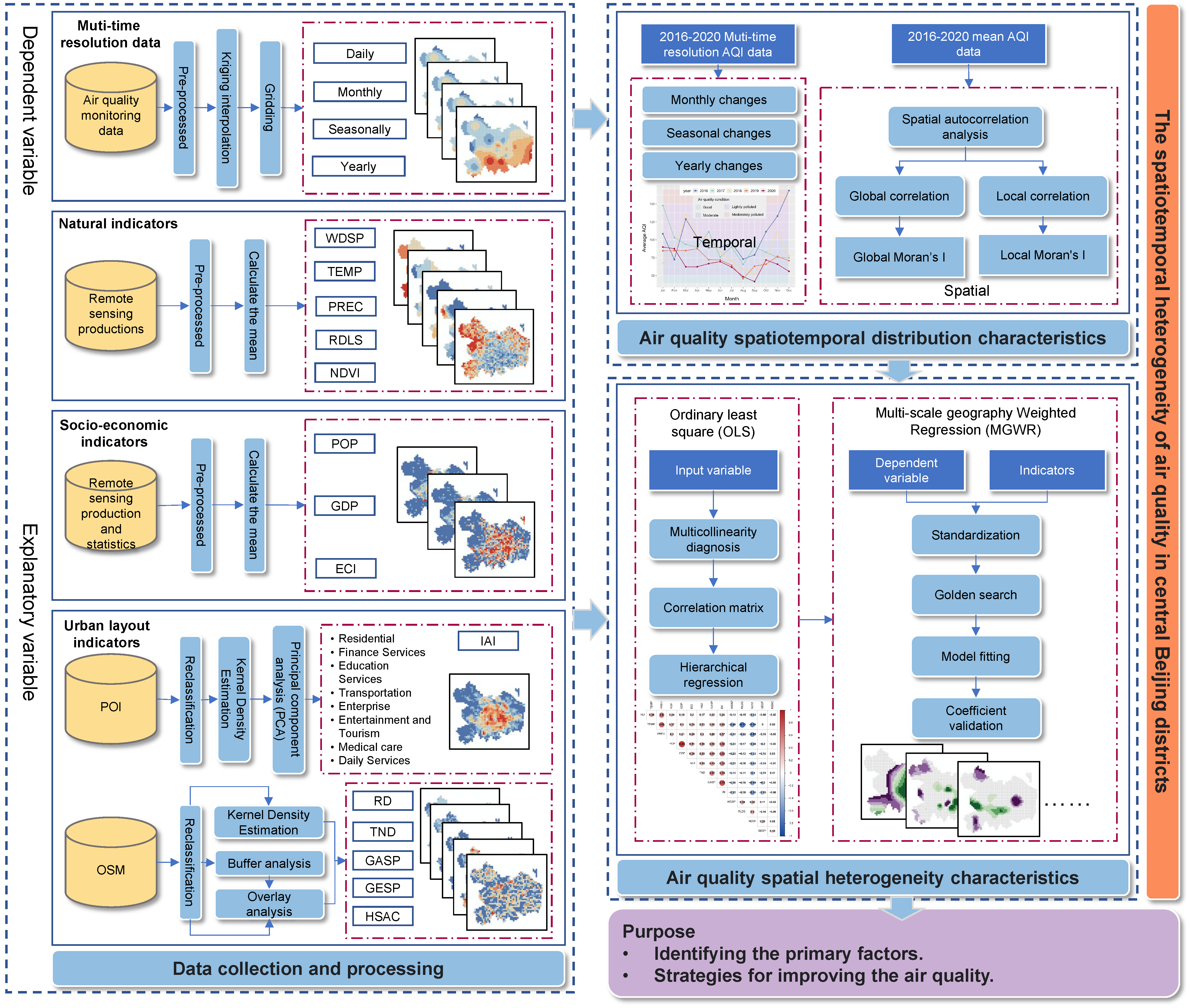
3. Methods and Models

The research framework of this article (Figure 2) encompasses the following aspects: (1) constructing an indicator system using urban air quality’s influencing factors based on natural environment, socio-economic, and urban layout dimensions; (2) conducting multi-temporal scale studies of air quality trends to analyze and compare the trends in the AQI at different time scales and using spatial autocorrelation to analyze the overall spatial distribution characteristics of the AQI; (3) Employing GWR and MGWR models to quantitatively analyze the impact strength and spatial heterogeneity of air quality driving factors, providing refined references for regional development.

3.1. IndicatorConstruction Module

Considering the natural environment, socio-economic factors, and urban spatial layout comprehensively, an evaluation indicator database for air quality driving factors at the urban scale has been constructed.

The Ordinary Kriging interpolation method is employed to interpolate discrete monitoring data, resulting in the distribution data of the AQI being used as the dependent variable. The Ordinary Kriging interpolation estimates that if there are $n$ known points $x_i\left(i=\mathrm{1,2},\cdots ,n\right)$ around a point, then the estimated value at point $x_0$ can be calculated using Equation (2):

$$Z\left(X_O\right)=\sum _{i=1}^n{\beta }_i·z\left(x_i\right)$$

(2)

$$\sum _{i=1}^n{\beta }_i=1$$

(3)

where ${\beta }_i$ is the weight assigned to $z\left(x_i\right)$ in the distribution. The weights are calculated using the Lagrange multipliers method, and the sum of the weights equals 1 (as stated in Equation (3)); $z\left(x_i\right)$ is the observed value at the known location $x_i$; $Z\left(x_0\right)$ is the estimated value at the estimation location $x_0$; and n is the number of actual observed values used to estimate ${Z(x}_0)$.

Natural environmental factors are composed of meteorological elements, topographic features, and vegetation cover. Meteorological factors include average temperature (TEMP), precipitation (PREC), and wind speed (WDSP). Wind speed data were also obtained by Ordinary Kriging interpolation, producing annual average values for 2016–2020. Topographic features are represented by the relief degree of land surface (RDLS), which describes the urban surface morphology. Vegetation cover is characterized by the NDVI.

The socio-economic characteristics used comprise population distribution (POP), the distribution of Gross Domestic Product (GDP), and energy consumption intensity (ECI). Nightlight remote sensing data represent energy consumption intensity.

Urban spatial layout is composed of the Industrial Agglomeration Index (IAI), traffic network density (TND), Residential Density (RD), Green Space Ratio (GESP), Grey Space Ratio (GASP), and Humidity Space Adjusted Capability (HSAC). Residential Density is used to identify areas with concentrated populations and relatively sparse areas. The Industrial Agglomeration Index reflects the spatial concentration of industries within the city. Based on the selected eight categories of POI data, urban functional areas are identified through a kernel density analysis. Subsequently, a Principal Component Analysis (PCA) is applied to these complex functional area classification data to derive key dimensions, resulting in the Industrial Agglomeration Index, which facilitates an intuitive understanding and analysis of the distribution of urban industries. Traffic network density reflects the aggregation of roads and railways within the study unit, and its calculation formula is as follows:

$$RD=({rail}_{len}+{road}_{len})/{grid}_{area}$$

(4)

where ${rail}_{len}$ is the total length of roads within the study unit, ${road}_{len}$ is the total length of railways within the study unit, and ${grid}_{area}$ is the area of the study unit.

The GESP and GASP represent the greenness space and floor area percentage in each grid, respectively. The urban humidity space is characterized by water bodies and analyzed using multilevel buffer zones. Buffer radii of 50 m, 100 m and 200 m are set sequentially, corresponding to the air quality regulation coefficients of 0.65, 0.25, and 0.1, respectively. Finally, the humidity space regulation capacity of each unit is calculated according to the following equation:

$$HSAC=\sum _{i=1}^n{x}_i·{\beta }_i$$

(5)

where ${\beta }_i$ is the adjustment factor and $x_i$ is the area of the buffer corresponding to ${\beta }_i$.

3.2. Spatial Distribution Feature Generation

Spatial autocorrelation is categorized into global autocorrelation and local autocorrelation. Global autocorrelation can be characterized by the Global Moran’s I statistic to characterize the overall spatial distribution of air quality. The formula is as follows:

$$I={\displaystyle \frac{n}{S_0}}{\displaystyle \frac{{\sum }_{i=1}^n\sum _{j=1}^n{w}_{i,j}{z}_i{z}_j}{{\sum }_{i=1}^n{z}_i^2}}$$

(6)

where $n$ is equal to the total number of elements, $S_0$ is the aggregation of all spatial weights, $z_i$ is the deviation between the attribute of element $i$ and its mean, and $w_{i,j}$ is the spatial weight between elements $i$ and $j$. A value > 0 indicates that there is a positive correlation in the spatial data, and a value < 0 indicates that there is a negative correlation in the spatial data. When the value is close to 0, there is no significant correlation.

Local Moran’s I values are categorized into spatial aggregation patterns of high–high (H-H), low–low (L-L), low–high (L-H), or high–low (H-L) based on aggregation. The calculation formula is as follows:

$$I_i={\displaystyle \frac{Z_i}{S^2}}\sum _{j\ne i}^n{w}_{i,j}{Z}_j$$

(7)

where $I_i$ is the local Moran’s I of region $i$, $S^2$ is the variance of all observations, $Z_i$ is the normalized observation, $w_{i,j}$ is the spatial weight between element $i$ and $j$, $Z_j$ is the standardized score of the attribute value of position $j$, and $n$ is the synthesis of all regions in the study area.

3.3. Spatial Heterogeneity Feature Generation

Spatial variation in the impact of different influencing factors on the AQI is analyzed using GWR and MGWR. GWR is a local modeling tool based on the optimization of global regression models, where each sampling location has its parameter within the following equation:

$$y_i={\beta }_0(u_i,v_i)+\sum _{j=1}^n{\beta }_j(u_i,v_i)x_{ij}+{\epsilon }_i$$

(8)

where $(u_i,v_i)$ are the coordinates of point $i$ in space, ${\beta }_j(u_i,v_i)$ is the regression coefficient of each variable at point $i$, ${\beta }_0(u_i,v_i)$ is a constant term, ${\epsilon }_i$ is the regression residual of the point $i$, and $n$ is the number of independent variables.

MGWR is an improved algorithm based on GWR, which can solve the problem of the GWR model defaulting to all the influencing factors playing a constant role on the spatial scale in the analysis of spatial heterogeneity, so that we can study the relationship between the influencing factors at different scales. The equation is as follows:

$$y_i={\beta }_{bw0}(u_i,v_i)+\sum _{j=1}^n{\beta }_{bwj}(u_i,v_i)x_{ij}+{\epsilon }_i$$

(9)

Each regression coefficient ${\beta }_{bwj}$ is obtained based on a local regression process and has different bandwidth settings, where $bw0$ is the intercept bandwidth, $bwj$ is the bandwidth of the variable $j$, and the remaining parameters are consistent with Equation (8).

To evaluate the effect of these two regression models, the coefficient of determination (R²), the corrected Akaike information criterion (AICc), and the residual sum of squares (RSS) are used as evaluation indicators.

4. Results and Discussion

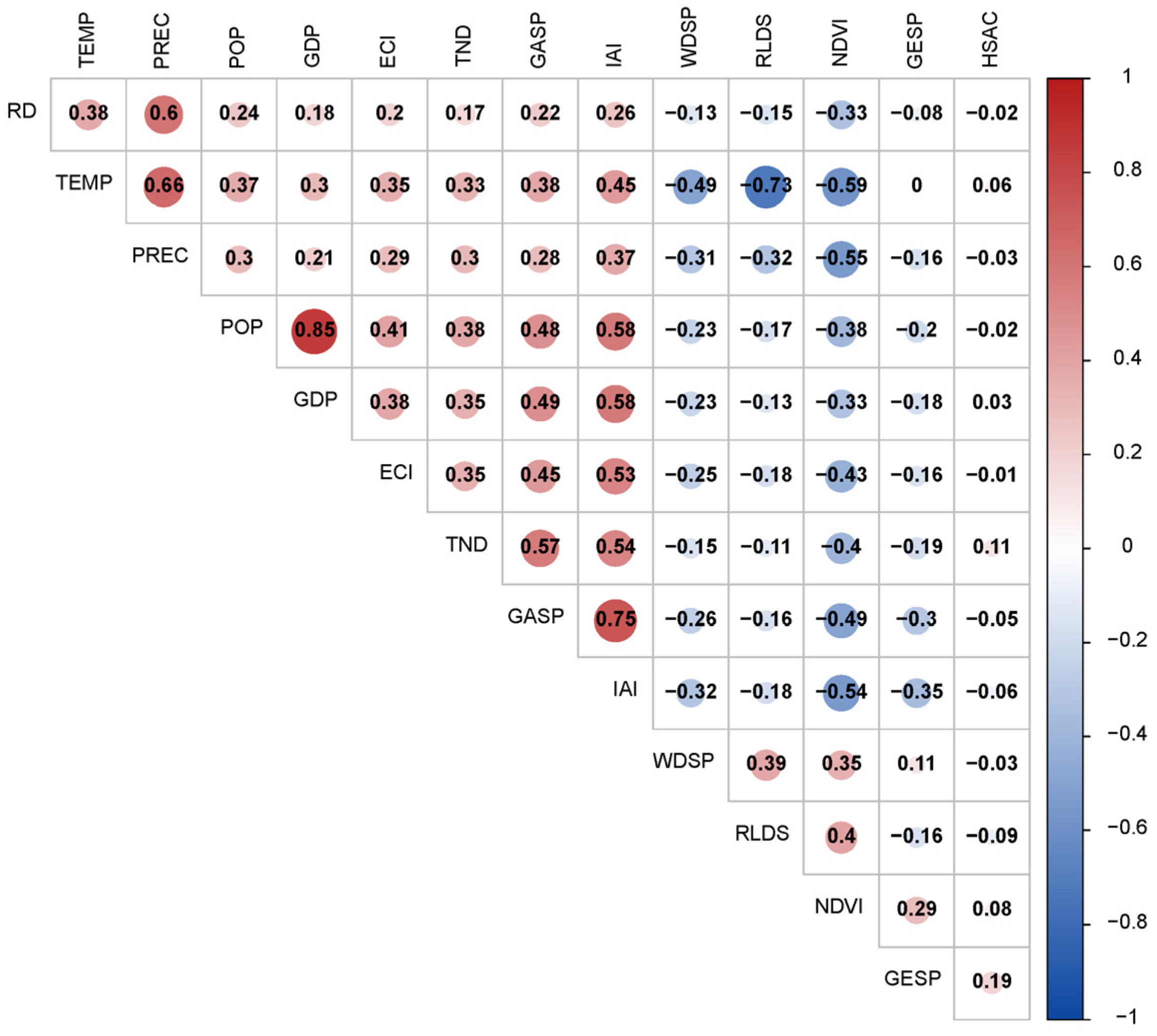
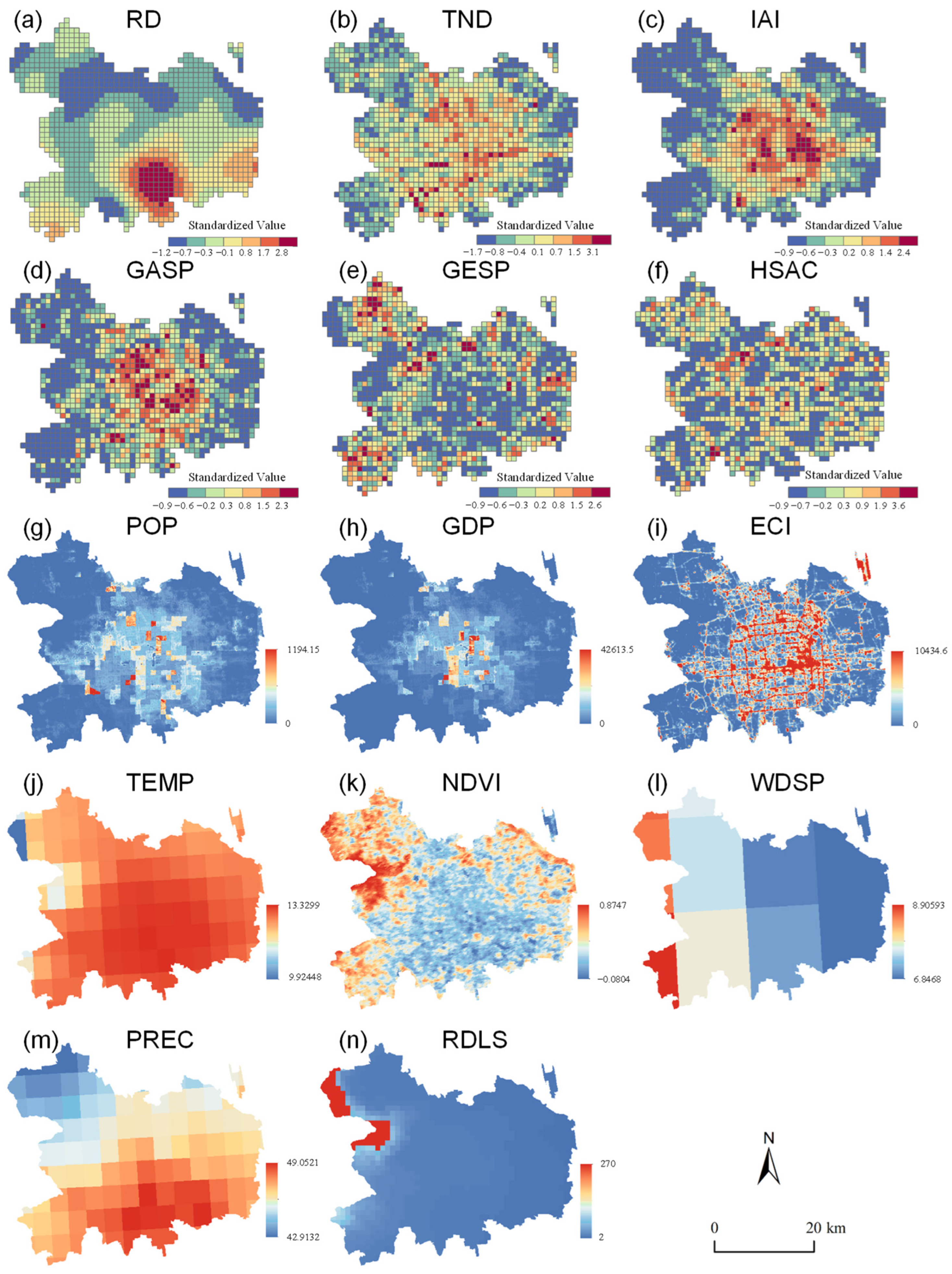
4.1. Dominant Impact Indicators

The air quality of the monitoring area is assessed using the average value of the historical data from each monitoring station over 5 years (Figure 3). The results indicate that the air quality in Fengtai District is the poorest, while that in Shijingshan District and Haidian District is the best. Chaoyang District, being large, shows minimal variation in its monitoring results and maintains a moderate air quality level. The eastern and western urban areas are the core areas of Beijing, exhibiting a high AQI in their north and south, but a low one in the middle. That is, the central area enjoys excellent air quality, whereas at the junction of peripheral urban areas it is generally lower.

The correlation analysis matrix (Figure 4) indicates that the correlation between POP and GDP is 0.85, and the correlation between IAI and GASP is 0.75, both of which show strong positive correlations. The correlation between TEMP and RDLS is −0.73, showing a strong negative correlation. A multicollinearity diagnosis further verifies whether these highly correlated indicators need to be eliminated. The diagnosis results (

Table 2. AQI-based explanatory variable index system and multicollinearity diagnostic results.

Indicator Category	Indicator	Abbreviation	Description	Unit	Collinearity Statistic
					Tolerance	VIF
Natural indicators	Wind speed	WDSP	Mean wind speed from 2016 to 2020	0.1 knots	0.720	1.390
	Temperature	TEMP	Mean temperature from 2016 to 2020	°C	0.215	4.659
	Precipitation	PREC	Mean precipitation from 2016 to 2020	mm	0.360	2.780
	Relief degree of land surface	RDLS	Comprehensive characterization of altitude and surface incision in 2014	\	0.383	2.613
	Normalized difference vegetation index	NDVI	Mean NDVI from 2016 to 2020	\	0.466	2.147
Socioeconomic indicators	Energy consumption intensity	ECI	Characterization using nighttime light remote sensing data in 2018	\	0.670	1.494
	Population	POP	Total population distribution	104 people	0.245	4.090
	Gross domestic product	GDP	Mean GDP from 2016 to 2020	104 yuan	0.248	4.034
Urban layout indicators	Industry aggregation index	IAI	Reflect the agglomeration of urban industries	\	0.304	3.295
	Transportation network density	TND	The ratio of road network length to unit area in each grid	m/km2	0.589	1.696
	Residential density	RD	Reflect the gathering situation of residential areas	\	0.618	1.617
	Green space percent	GESP	Green space area to unit ratio	%	0.736	1.358
	Gray space percent	GASP	Building area to unit ratio	%	0.381	2.627
	Humidity space adjustment capability	HSAC	Reflects the ability of wetlands to purify the air quality	\	0.907	1.103

) show that the VIF of all indicators is less than 5, proving that there are no collinearity issues and that each indicator can independently explain its impact on air quality.

The spatial distribution of each variable reflects the spatial distribution heterogeneity of the driving factors (Figure 5). As an indicator of urban spatial pattern, Figure 5a–f show the most pronounced spatial heterogeneity.

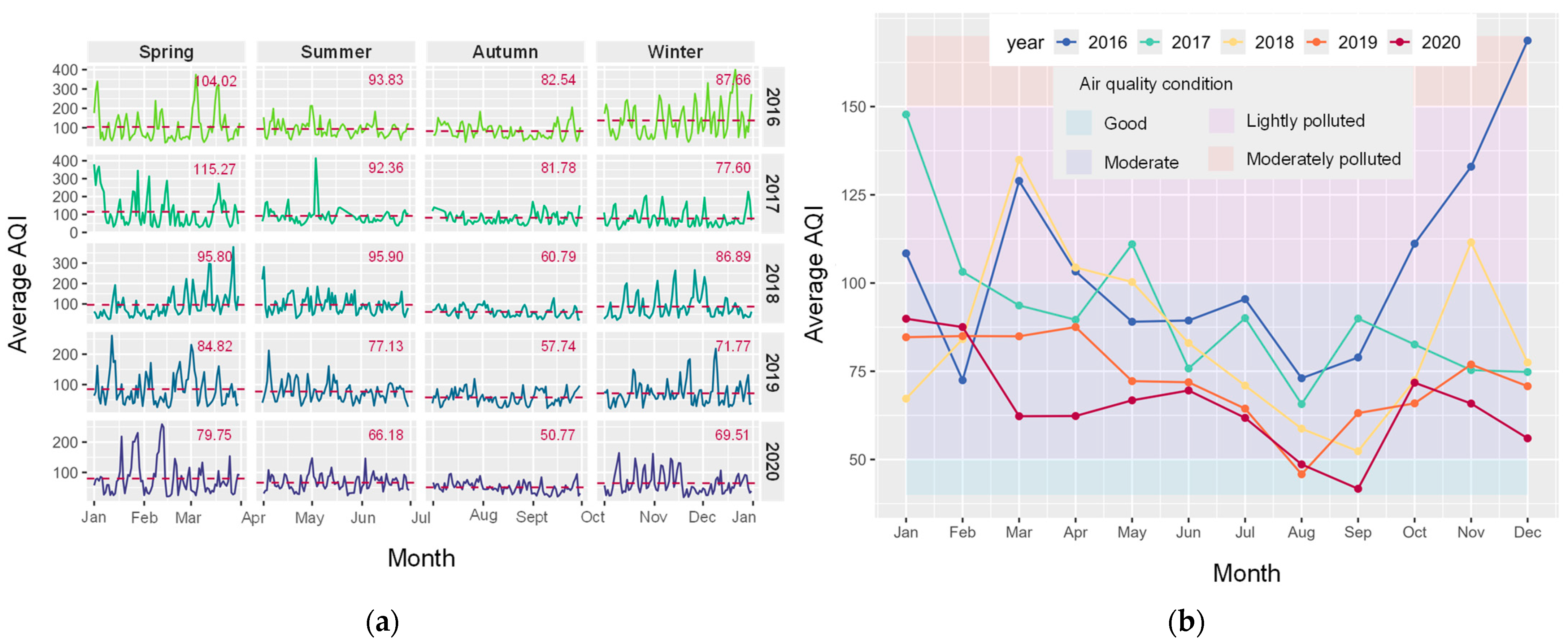
4.2. Temporal Characteristics of the AQI

From 2016 to 2020, the annual AQI of the study area showed an overall downward trend (Figure 6a). The AQI followed a U-shaped variation across seasons (Figure 6b) and in spring was generally higher. Subsequently, in summer, the increase in rainfall usually helped to reduce pollutants in the air, leading to a decrease in AQI values. In autumn, the AQI remained at a low level, but, in winter, with the increase in heating demand, coal pollution caused the AQI to rise again. This seasonal U-shaped pattern in AQI variations indicates a complex interplay of various environmental and human factors within Beijing’s urban environment. It underscores the need for dynamic and season-specific approaches to regulating air quality, considering natural and anthropogenic factors that affect pollution levels throughout the year. For instance, a stricter control of construction dust in spring and reducing coal use in winter are necessary measures.

The seasonal variation of monthly average AQI values from 2016 to 2020 highlights the difference in monthly air quality (Figure 6b). From 2016 to 2018, air quality was mainly concentrated in the range of moderate to mild pollution. From 2019 to 2020, air quality was mainly distributed between the good and medium grades, showing a significant increase in the proportion of air quality improvement.

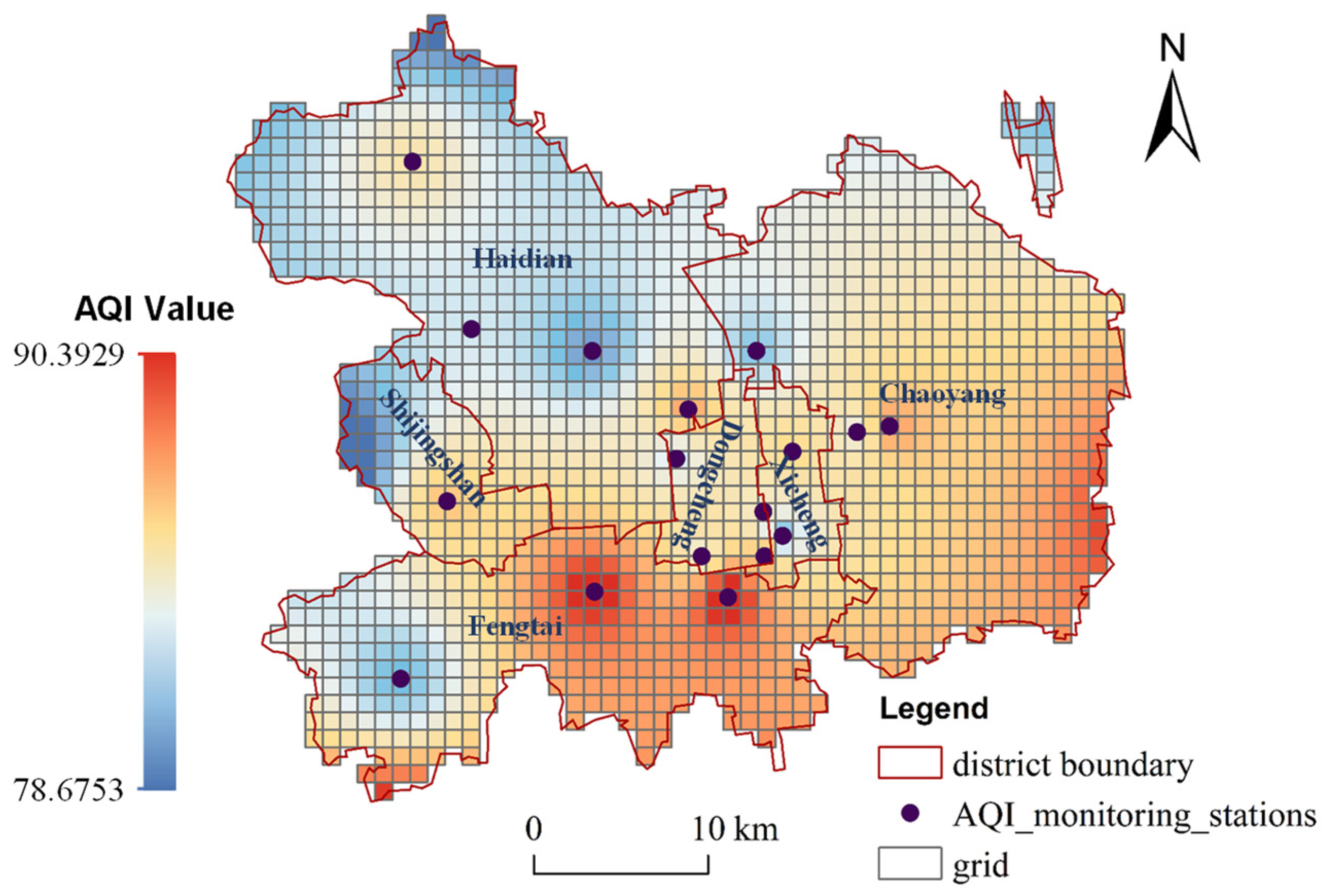
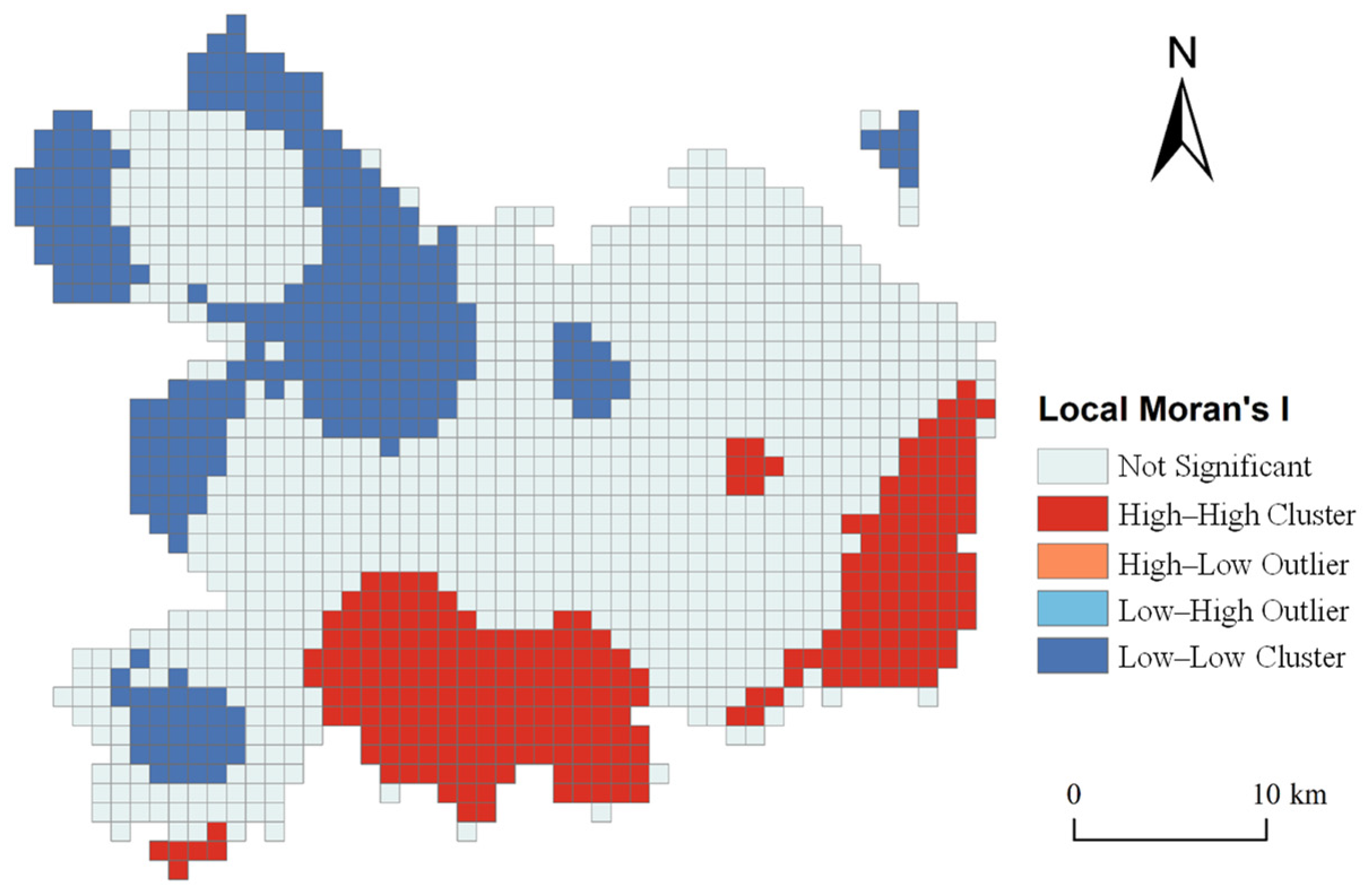
4.3. Spatial Characteristics of AQI

The global Moran’s I = 0.922, indicating that there is a significant positive spatial autocorrelation in the AQIs in the study area. Local spatial autocorrelation analysis identified cold and hot spots (Figure 7). The population in the hot spot area is dense, with high coal consumption for heating in winter and high power consumption for cooling in summer, resulting in substantial air pollutant emissions. In addition, the plain terrain facilitates the spread of air pollutants between regions, which eventually leads to the accumulation of high AQI values. Multiple continuous grids in the Haidian District in the northwest of the study area belong to the cold spot area, and their AQI value is low, showing a low–low cluster and high local correlation. This is mainly because Haidian District contains a number of large national parks; the northwest possesses a high greening rate and strong air purification capacity.

4.4. Comparative Analysis of GWR and MGWR Results

The MGWR model performs better than the traditional GWR model. Specifically, the MGWR model has a significantly higher coefficient of determination (R² = 0.985) and adjusted coefficient of determination (Adjusted R² = 0.975), which means that the model has significant explanatory power for almost all variables. Additionally, the MGWR model has a lower Akaike information criterion correction value (AICc = 104.817) and residual sum of squares (RSS = 20.318), indicating that it has higher accuracy and a lower error in fitting data and can better capture and explain the local variability of spatial data.

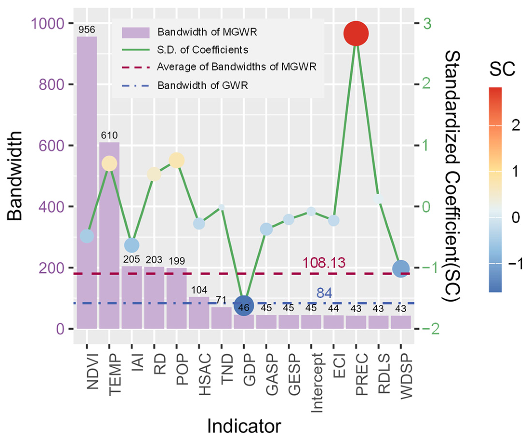
4.4.1. Bandwidth Analysis Driving Factors

The optimal bandwidth of each variable is generated by the MGWR and GWR models, and the standardized parameter estimation corresponding to the MGWR model varies (Figure 8), where the optimal bandwidth of the GWR model is 84, and the average of the 15 bandwidths of the MGWR model is 180.13. MGWR simulates the effects of variables on different spatial scales, resulting in varying optimal bandwidths. The larger the bandwidth, the greater the overall impact of the variable on the air quality in a space, the higher the degree of spatial stability, and the smaller the spatial heterogeneity. On the contrary, variables with smaller bandwidths have a significant impact on air quality locally, with a higher degree of spatial non-stationarity and spatial heterogeneity. The results show that NDVI and TEMP have large bandwidths and low spatial heterogeneity. The bandwidths of IAI, RD, and POP are slightly higher than the average bandwidth, indicating that the spatial heterogeneity of these three variables is at a medium level. The nine variables HSAC, TND, GDP, GASP, GESP, ECI, PREC, RDLS, and WDSP have small bandwidths and significant heterogeneity in their impact on air quality.

The standardized coefficient (SC) can reflect the influence of variables on air quality. The SC values of TND and RDLS are close to 0, suggesting that these two variables have negligible effects on air quality. PREC > POP > TEMP > RD > 0.5, indicating a significant positive relationship between these four variables and the AQI, indicating that these four variables are important factors that aggravate air pollution. GDP < WDSP < IAI < −0.5 < NDVI < GASP < HASC < ECI < GESP < 0, showing a negative relationship, where higher values correlate with a lower AQI, implying a positive effect on the improvement of air quality.

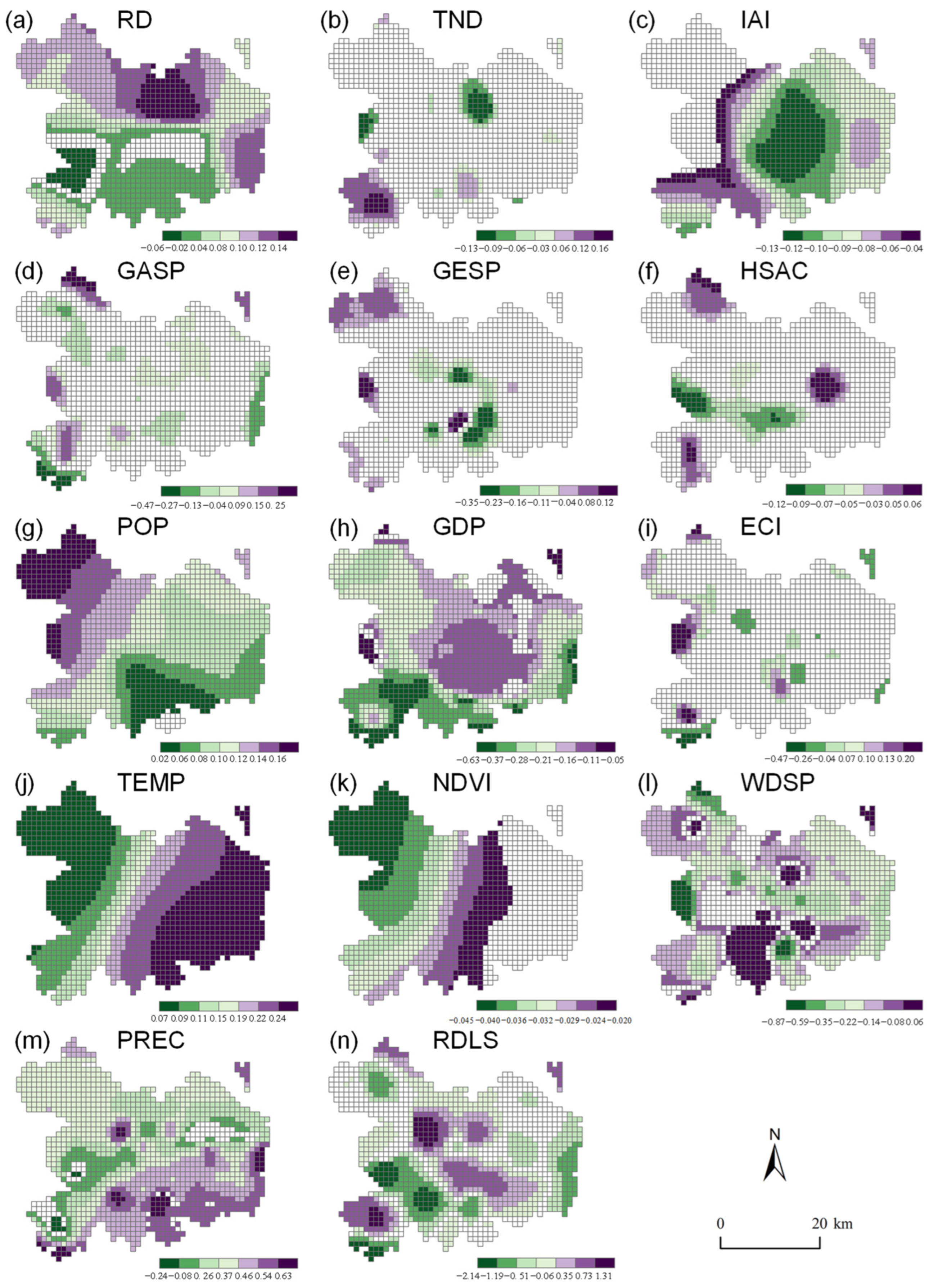
4.4.2. Spatial Heterogeneity Analysis of Driving Factors

The local regression coefficients of each variable and their significance were analyzed to assess the global impact of each variable on urban air quality (

Table 3. Statistical characteristics of MGWR coefficients.

Indicator Category	Indicator	MGWR Coefficients			Percentage of Grids by Significance (95% Level) of t-Test
		Min	Max	Mean	p ≤ 0.05 (%)	+ (%)	− (%)
NI	NDVI	−0.043	−0.010	−0.026	70.55	0	100
	PREC	−0.242	0.877	0.404	93.49	99.31	0.69
	RDLS	−2.143	2.137	0.053	70.98	58.71	41.29
	TEMP	0.069	0.257	0.173	100	100	0
	WDSP	−0.872	0.468	−0.126	85.53	13.11	86.89
SEI	POP	0.020	0.209	0.108	98.77	100	0
	ECI	−0.466	0.286	0.015	20.11	74.46	25.54
	GDP	−0.634	0.373	−0.178	91.90	2.05	97.95
ULI	GESP	−0.346	0.188	−0.009	25.11	47.84	52.16
	HSAC	−0.119	0.082	−0.004	26.34	47.80	52.20
	GASP	−0.464	0.435	0.003	33.72	54.94	45.06
	TND	−0.140	0.200	0.009	17.44	63.07	36.93
	RD	−0.065	0.186	0.076	87.84	95.30	4.70
	IAI	−0.126	0.034	−0.072	76.70	0	100

). The results indicate that at a significance level of p ≤ 0.05, the parameter estimates for PREC, TEMP, POP, and RD are significant across more than 85% of the region, demonstrating a strong positive correlation. The parameter estimates for NDVI, WDSP, GDP, and IAI are significant across more than 70% of the region, indicating a pronounced negative correlation. Among the remaining variables, the positive effects of RDLS, GASP, and TND on the AQI outweigh the negative effects, while GESP and HSAC show stronger negative effects than positive ones.

The spatial distribution of the standardized coefficients of the MGWR model variables (Figure 9) illustrates the diverse characteristics of the spatial heterogeneity among these variables. In terms of urban spatial layout indicators, RD (Figure 9a) exhibits the most significant positive correlation. Negative coefficients are concentrated in the south of Shijingshan District and the northwest of Fengtai District, while positive coefficients are concentrated in Haidian District, Chaoyang District, and the border area and eastern part of Chaoyang District. TND (Figure 9b) shows a negative correlation in the northwest of Chaoyang District and a positive correlation in the west of Fengtai District, suggesting that, despite the current roads, traffic network density in Fengtai District is low and traffic pollution emissions are serious. IAI is the most significant correlation variable (Figure 9c), with its effect weakening from the center of Dongcheng District and Xicheng District to the surrounding areas, indicating a relatively balanced industrial distribution in the study area. Figure 9d,e depict the heterogeneity of the impact of urban green spaces, gray spaces, and humid spaces on air quality, reflecting the influence of urban architecture and ecological environment configurations. Overall, the positive effect of GASP in the study area outweighs the negative effect, potentially due to the concentrated distribution of buildings forming a local heat island effect which elevates air pollutant concentrations and hinders their dispersion. Conversely, GESP and HSAC show a contrasting effect to GASP. Thus, increasing urban green space and wetlands remain crucial strategies for urban air purification.

In terms of the socio-economic indicators, POP (Figure 9g) exhibits a notable positive correlation, showing an increasing trend from the southeast to the northwest across the city’s six districts. GDP (Figure 9h) shows a significant negative correlation, and the correlation is generally manifested as an increasing trend from the middle of the study area to the surrounding areas. The overall performance of ECI (Figure 9i) is positively correlated, suggesting that reducing the current intensity of energy consumption, especially electrical energy, will aid in improving air quality under the current conditions.

Among the natural environment indicators, TEMP (Figure 9j) and NDVI (Figure 9k) show significant positive and negative correlations, respectively, and their positive correlation is stronger than their negative correlation. Their positive correlation increases from west to east, as the distribution of vegetation has a regulating effect on surface temperature. The influence of WDSP on the AQI is negatively correlated as a whole. Areas with a high wind speed are helpful for their ability to diffuse pollutants and reduce the accumulation of pollutants. PREC (Figure 9m) demonstrates a strong overall positive correlation, which may be related to the research scale. This study considers the average effect in a long time series, ignoring the relationship between rainfall and the AQI over time. RDLS (Figure 9n) has an almost negligible effect on the AQI because pollutants are not easy to gather in undulating flat areas. However, the spatial distribution of the regression coefficient of this variable has a certain heterogeneity, possibly due to the distribution of buildings.

4.5. Research Comparation

This study is highly consistent with existing relevant research findings. Tian et al. analyzed the temporal and spatial variations in air quality in Beijing from 2001 to 2017, finding a negative correlation between vegetation coverage and air quality and a positive correlation between energy consumption intensity and air quality. This aligns with our findings, wherein NDVI negatively impacts air quality and ECI positively impacts air quality, indicating that increasing vegetation coverage and reducing energy consumption intensity are effective measures to improve air quality [43]. Li et al. evaluated the effectiveness of two air quality improvement action plans in Beijing, namely the “Clean Air Action” and “Comprehensive Action”, and found that, under government intervention, coordinated efforts between economic growth and pollution control significantly improved air quality. This is consistent with our research conclusion that strict industrial emission control and the optimization of energy structures can effectively improve air quality [44]. Ban et al. explored the impact of urbanization on aerosol optical depth, revealing a close correlation between land surface temperature, land use type, and aerosol concentration. This correlates with our findings on the impact of TEMP and ULI on air quality, highlighting the significant effects of land use changes and temperature variations during urbanization processes [45]. Zhan et al. used an MGWR to examine the relationship between green space patterns and PM2.5 exposure, demonstrating that green spaces mitigate PM2.5 exposure risks at larger scales. Our study similarly employed the MGWR model and found that the GESP has a significant positive impact on air quality, supporting the effectiveness of increasing urban green spaces as a measure to improve air quality [46].

Compared to these related studies, this research provides a more comprehensive and systematic analysis by considering multiple factors such as the natural environment, socio-economic conditions, and urban spatial layout. This approach is beneficial for offering more specific guidance and references to governments and relevant departments in the practice of air pollution prevention and control. Its scientific value lies in its multidimensional and multi-scale perspective, which reveals the key factors affecting air quality and their interaction mechanisms. This enriches existing environmental science theories and offers significant references for future research in related fields.

4.6. Strategies and Suggestions

Given this comprehensive strategy for improving air quality in the study area, it is necessary to address the issue from the three key dimensions of natural environmental protection, sustainable socio-economic development, and urban spatial layout optimization. From a natural environment perspective, emphasizing the role of WDSP in promoting the diffusion of air pollutants through rational urban planning, such as building ventilation corridors, optimizing building layouts, and enhancing air circulation capacity, is crucial. Additionally, increasing urban vegetation coverage (NDVI) not only helps regulate urban temperature and reduce the heat island effect but also directly improves air quality. In terms of socio-economic characteristics, reducing the ECI and balancing the relationship between POP and economic growth (GDP) are vital. Implementing policies that promote energy efficiency and the use of renewable energy sources can significantly reduce pollution. In this process, government interventions, such as implementing strict emission standards and incentive measures, can enhance the effectiveness of policy implementation. Optimizing urban spatial layout involves addressing the impact of industrial activities (IAI) and the traffic network (TND) on air quality. By strictly controlling industrial emissions, optimizing traffic structures, encouraging public transportation use, expanding the GESP, and improving the GASP and HSAC, these strategies can significantly reduce air pollution sources and enhance the city’s ecosystem services, creating a more livable environment. Integrating these measures provides specific guidance for urban planning and policy-making to achieve sustainable air quality improvements.

5. Conclusions

This paper analyzes the spatial and temporal distribution characteristics of the AQI in the study area and explores the relationships between and spatial heterogeneity of the driving factors affecting urban air quality from three aspects—the natural environment, social economy, and urban spatial layout—based on multi-source data. The main conclusions are as follows: (1) The spatiotemporal distribution of air quality in the study area shows a certain regularity. Temporally, the overall air quality has been improving year by year and follows a U-shaped seasonal pattern; that is, spring and winter are the high-value seasons of the AQI, while summer and autumn are low. Spatially, the high-value aggregation areas of the AQI are distributed in the eastern part of Chaoyang District and Fengtai District. Its low-value aggregation areas are distributed in the central and northern parts of Haidian District and the western part of Shijingshan District. (2) The fitting performance of the MGWR model is better than that of the GWR. The bandwidth of the MGWR model can dynamically reflect the spatial effect of variables, making it suitable for identifying the dominant factors affecting air quality and their spatial effect differences using multivariate regression. The standardized parameter estimates obtained from the MGWR model reflect that the influence of TND and RDLS, of the variables used in this study, is low. Among the variables with a significant positive relationship with the AQI, their degree of influence is PREC > POP > TEMP > RD > 0.5. Among the variables showing a negative relationship with the AQI, their degree of influence is as follows GDP < WDSP < IAI < −0.5 < NDVI < GASP < HASC < ECI < GESP < 0. (3) The intensity and spatial heterogeneity of these driving factors were identified. The strong spatial heterogeneity variables with significant positive effects on air quality are NDVI, GDP, and HSAC, while those with notable negative effects include POP, TEMP, and RD.

Therefore, in the process of urban planning, it is necessary to coordinate the relationship between population and development quality, the natural environment, and the built environment, from the perspective of regional differences, to improve air quality. Furthermore, the principles of sustainable development should be emphasized by optimizing land use, increasing green space coverage, enhancing the efficiency of public transportation systems, and promoting the construction of green buildings to reduce pollution and resource consumption. The government should actively intervene in environmental governance by enacting and enforcing strict environmental regulations, providing financial support and incentives, and promoting innovations in environmental protection technologies to ensure the effectiveness and longevity of environmental measures [47,48]. By comprehensively considering social, economic, and environmental factors, we can formulate long-term effective planning strategies that not only meet current needs but also lay a solid foundation for future sustainable development [9,49].

However, this study has certain limitations, which are reflected in the analysis of the heterogeneity of driving factors on the missing time scale. In future studies, researchers or city managers may wish to explore the spatiotemporal distribution characteristics of the AQI driving factors in a time series for an indicative level of the natural environment, socio-economy, and urban layout. This allows for the construction of dynamic and specific MGWR models that will help each specific area to scientifically develop refined air quality management countermeasures.

References

1. Cohen, B. Urbanization in Developing Countries: Current Trends, Future Projections, and Key Challenges for Sustainability. Technol. Soc. 2006, 28, 63–80. [Google Scholar] [CrossRef]
2. Li, R.; Cui, L.; Li, J.; Zhao, A.; Fu, H.; Wu, Y.; Zhang, L.; Kong, L.; Chen, J. Spatial and Temporal Variation of Particulate Matter and Gaseous Pollutants in China during 2014–2016. Atmos. Environ. 2017, 161, 235–246. [Google Scholar] [CrossRef]
3. Zhou, D.; Zhao, S.; Zhang, L.; Sun, G.; Liu, Y. The Footprint of Urban Heat Island Effect in China. Sci. Rep. 2015, 5, 11160. [Google Scholar] [CrossRef] [PubMed]
4. Horton, R.M.; Mankin, J.S.; Lesk, C.; Coffel, E.; Raymond, C. A Review of Recent Advances in Research on Extreme Heat Events. Curr. Clim. Chang. Rep. 2016, 2, 242–259. [Google Scholar] [CrossRef]
5. Fang, C.; Liu, H.; Li, G.; Sun, D.; Miao, Z. Estimating the Impact of Urbanization on Air Quality in China Using Spatial Regression Models. Sustainability 2015, 7, 15570–15592. [Google Scholar] [CrossRef]
6. Kuhlman, T.; Farrington, J. What Is Sustainability? Sustainability 2010, 2, 3436–3448. [Google Scholar] [CrossRef]
7. Chan, C.K.; Yao, X. Air Pollution in Mega Cities in China. Atmos. Environ. 2008, 42, 1–42. [Google Scholar] [CrossRef]
8. Huang, R.-J.; Zhang, Y.; Bozzetti, C.; Ho, K.-F.; Cao, J.-J.; Han, Y.; Daellenbach, K.R.; Slowik, J.G.; Platt, S.M.; Canonaco, F. High Secondary Aerosol Contribution to Particulate Pollution during Haze Events in China. Nature 2014, 514, 218–222. [Google Scholar] [CrossRef]
9. Yuan, G.; Yang, W. Evaluating China’s Air Pollution Control Policy with Extended AQI Indicator System: Example of the Beijing-Tianjin-Hebei Region. Sustainability 2019, 11, 939. [Google Scholar] [CrossRef]
10. Hu, J.; Ying, Q.; Wang, Y.; Zhang, H. Characterizing Multi-Pollutant Air Pollution in China: Comparison of Three Air Quality Indices. Environ. Int. 2015, 84, 17–25. [Google Scholar] [CrossRef]
11. Zhang, J.; Cui, K.; Wang, Y.-F.; Wu, J.-L.; Huang, W.-S.; Wan, S.; Xu, K. Temporal Variations in the Air Quality Index and the Impact of the COVID-19 Event on Air Quality in Western China. Aerosol. Air Qual. Res. 2020, 20, 1552–1568. [Google Scholar] [CrossRef]
12. World Health Organization. WHO Global Air Quality Guidelines: Particulate Matter (PM2. 5 and PM10), Ozone, Nitrogen Dioxide, Sulfur Dioxide and Carbon Monoxide; World Health Organization: Geneva, Switzerland, 2021; ISBN 92-4-003422-6. [Google Scholar]
13. Shen, F.; Ge, X.; Hu, J.; Nie, D.; Tian, L.; Chen, M. Air Pollution Characteristics and Health Risks in Henan Province, China. Environ. Res. 2017, 156, 625–634. [Google Scholar] [CrossRef] [PubMed]
14. Du, X.; Chen, R.; Meng, X.; Liu, C.; Niu, Y.; Wang, W.; Li, S.; Kan, H.; Zhou, M. The Establishment of National Air Quality Health Index in China. Environ. Int. 2020, 138, 105594. [Google Scholar] [CrossRef] [PubMed]
15. Liao, T.; Jiang, W.; Ouyang, Z.; Hu, S.; Wu, J.; Zhao, B.; Wang, B.; Wang, S.; Sun, Y. Evaluation of the Health Risk of Air Pollution in Major Chinese Cities Using a Risk-Based, Multi-Pollutant Air Quality Health Index during 2014–2018. Air Qual. Atmos. Health 2021, 14, 1605–1617. [Google Scholar] [CrossRef]
16. Xu, L.; Zhou, J.; Guo, Y.; Wu, T.; Chen, T.; Zhong, Q.; Yuan, D.; Chen, P.; Ou, C. Spatiotemporal Pattern of Air Quality Index and Its Associated Factors in 31 Chinese Provincial Capital Cities. Air Qual. Atmos. Health 2017, 10, 601–609. [Google Scholar] [CrossRef]
17. Zhang, X.; Gong, Z. Spatiotemporal Characteristics of Urban Air Quality in China and Geographic Detection of Their Determinants. J. Geogr. Sci. 2018, 28, 563–578. [Google Scholar] [CrossRef]
18. Jiang, W.; Wang, Y.; Tsou, M.-H.; Fu, X. Using Social Media to Detect Outdoor Air Pollution and Monitor Air Quality Index (AQI): A Geo-Targeted Spatiotemporal Analysis Framework with Sina Weibo (Chinese Twitter). PLoS ONE 2015, 10, e0141185. [Google Scholar] [CrossRef] [PubMed]
19. Tan, S.; Xie, D.; Ni, C.; Zhao, G.; Shao, J.; Chen, F.; Ni, J. Spatiotemporal Characteristics of Air Pollution in Chengdu-Chongqing Urban Agglomeration (CCUA) in Southwest, China: 2015–2021. J. Environ. Manag. 2023, 325, 116503. [Google Scholar] [CrossRef] [PubMed]
20. Shi, K.; Chen, Y.; Li, L.; Huang, C. Spatiotemporal Variations of Urban CO2 Emissions in China: A Multiscale Perspective. Appl. Energy 2018, 211, 218–229. [Google Scholar] [CrossRef]
21. Wu, C.; Hu, W.; Zhou, M.; Li, S.; Jia, Y. Data-Driven Regionalization for Analyzing the Spatiotemporal Characteristics of Air Quality in China. Atmos. Environ. 2019, 203, 172–182. [Google Scholar] [CrossRef]
22. Fotheringham, A.S.; Yue, H.; Li, Z. Examining the Influences of Air Quality in China’s Cities Using Multi-scale Geographically Weighted Regression. Trans. GIS 2019, 23, 1444–1464. [Google Scholar] [CrossRef]
23. Xu, W.; Tian, Y.; Liu, Y.; Zhao, B.; Liu, Y.; Zhang, X. Understanding the Spatial-Temporal Patterns and Influential Factors on Air Quality Index: The Case of North China. Int. J. Environ. Res. Public Health 2019, 16, 2820. [Google Scholar] [CrossRef] [PubMed]
24. Miao, L.; Liu, C.; Yang, X.; Kwan, M.-P.; Zhang, K. Spatiotemporal Heterogeneity Analysis of Air Quality in the Yangtze River Delta, China. Sustain. Cities Soc. 2022, 78, 103603. [Google Scholar] [CrossRef]
25. Lu, X.; Yao, T.; Fung, J.C.; Lin, C. Estimation of Health and Economic Costs of Air Pollution over the Pearl River Delta Region in China. Sci. Total Environ. 2016, 566, 134–143. [Google Scholar] [CrossRef] [PubMed]
26. Yuan, J.; Wang, X.; Feng, Z.; Zhang, Y.; Yu, M. Spatiotemporal Variations of Aerosol Optical Depth and the Spatial Heterogeneity Relationship of Potential Factors Based on the Multi-Scale Geographically Weighted Regression Model in Chinese National-Level Urban Agglomerations. Remote Sens. 2023, 15, 4613. [Google Scholar] [CrossRef]
27. Guo, Y.; Tang, Q.; Gong, D.-Y.; Zhang, Z. Estimating Ground-Level PM2. 5 Concentrations in Beijing Using a Satellite-Based Geographically and Temporally Weighted Regression Model. Remote Sens. Environ. 2017, 198, 140–149. [Google Scholar] [CrossRef]
28. Wang, Q.; Feng, H.; Feng, H.; Yu, Y.; Li, J.; Ning, E. The Impacts of Road Traffic on Urban Air Quality in Jinan Based GWR and Remote Sensing. Sci. Rep. 2021, 11, 15512. [Google Scholar] [CrossRef] [PubMed]
29. Wang, Z.; Ma, P.; Zhang, L.; Chen, H.; Zhao, S.; Zhou, W.; Chen, C.; Zhang, Y.; Zhou, C.; Mao, H. Systematics of Atmospheric Environment Monitoring in China via Satellite Remote Sensing. Air Qual. Atmos. Health 2021, 14, 157–169. [Google Scholar] [CrossRef]
30. Zheng, S.; Wang, J.; Sun, C.; Zhang, X.; Kahn, M.E. Air Pollution Lowers Chinese Urbanites’ Expressed Happiness on Social Media. Nat. Hum. Behav. 2019, 3, 237–243. [Google Scholar] [CrossRef]
31. Lin, B.; Zhu, J. Changes in Urban Air Quality during Urbanization in China. J. Clean. Prod. 2018, 188, 312–321. [Google Scholar] [CrossRef]
32. Zhao, S.; Yu, Y.; Yin, D.; He, J.; Liu, N.; Qu, J.; Xiao, J. Annual and Diurnal Variations of Gaseous and Particulate Pollutants in 31 Provincial Capital Cities Based on in Situ Air Quality Monitoring Data from China National Environmental Monitoring Center. Environ. Int. 2016, 86, 92–106. [Google Scholar] [CrossRef] [PubMed]
33. Zhu, Y.; Wang, J.; Meng, B.; Ji, H.; Wang, S.; Zhi, G.; Liu, J.; Shi, C. Quantifying Spatiotemporal Heterogeneities in PM2. 5-Related Health and Associated Determinants Using Geospatial Big Data: A Case Study in Beijing. Remote Sens. 2022, 14, 4012. [Google Scholar] [CrossRef]
34. Sun, Z.; Zhan, D.; Jin, F. Spatio-Temporal Characteristics and Geographical Determinants of Air Quality in Cities at the Prefecture Level and above in China. Chin. Geogr. Sci. 2019, 29, 316–324. [Google Scholar] [CrossRef]
35. Grzędzicka, E. Is the Existing Urban Greenery Enough to Cope with Current Concentrations of PM2.5, PM10 and CO2? Atmos. Pollut. Res. 2019, 10, 219–233. [Google Scholar] [CrossRef]
36. Ma, L.; Wu, J.; Li, W.; Peng, J.; Liu, H. Evaluating Saturation Correction Methods for DMSP/OLS Nighttime Light Data: A Case Study from China’s Cities. Remote Sens. 2014, 6, 9853–9872. [Google Scholar] [CrossRef]
37. Chen, J.; Wang, B.; Huang, S.; Song, M. The Influence of Increased Population Density in China on Air Pollution. Sci. Total Environ. 2020, 735, 139456. [Google Scholar] [CrossRef]
38. Li, F.; Zhou, T.; Lan, F. Relationships between Urban Form and Air Quality at Different Spatial Scales: A Case Study from Northern China. Ecol. Indic. 2021, 121, 107029. [Google Scholar] [CrossRef]
39. Liu, J.; Ding, W. Spatial and Temporal Coupling Characteristics of Industrial Structure Optimization and Air Quality in Chinese Cities and Multi-Scale Driver Analysis. Environ. Sci. Pollut. Res. 2023, 30, 83888–83902. [Google Scholar] [CrossRef]
40. Rao, Y.; Wu, C.; He, Q. The Antagonistic Effect of Urban Growth Pattern and Shrinking Cities on Air Quality: Based on the Empirical Analysis of 174 Cities in China. Sustain. Cities Soc. 2023, 97, 104752. [Google Scholar] [CrossRef]
41. Singh, K.P.; Gupta, S.; Kumar, A.; Shukla, S.P. Linear and Nonlinear Modeling Approaches for Urban Air Quality Prediction. Sci. Total Environ. 2012, 426, 244–255. [Google Scholar] [CrossRef]
42. Zhang, L.; Tian, X.; Zhao, Y.; Liu, L.; Li, Z.; Tao, L.; Wang, X.; Guo, X.; Luo, Y. Application of Nonlinear Land Use Regression Models for Ambient Air Pollutants and Air Quality Index. Atmos. Pollut. Res. 2021, 12, 101186. [Google Scholar] [CrossRef]
43. Tian, Y.; Jiang, Y.; Liu, Q.; Xu, D.; Zhao, S.; He, L.; Liu, H.; Xu, H. Temporal and Spatial Trends in Air Quality in Beijing. Landsc. Urban Plan. 2019, 185, 35–43. [Google Scholar] [CrossRef]
44. Li, W.; Shao, L.; Wang, W.; Li, H.; Wang, X.; Li, Y.; Li, W.; Jones, T.; Zhang, D. Air Quality Improvement in Response to Intensified Control Strategies in Beijing during 2013–2019. Sci. Total Environ. 2020, 744, 140776. [Google Scholar] [CrossRef] [PubMed]
45. Ban, Y.; Liu, X.; Yin, Z.; Li, X.; Yin, L.; Zheng, W. Effect of Urbanization on Aerosol Optical Depth over Beijing: Land Use and Surface Temperature Analysis. Urban Clim. 2023, 51, 101655. [Google Scholar] [CrossRef]
46. Zhan, Q.; Yang, C.; Liu, H. How Do Greenspace Landscapes Affect PM2.5 Exposure in Wuhan? Linking Spatial-Nonstationary, Annual Varying, and Multiscale Perspectives. Geo-Spat. Inf. Sci. 2024, 27, 95–110. [Google Scholar] [CrossRef]
47. Wang, M.-X.; Huang, L.; Chen, Z.-M. The Impact of Green Financial Policy on the Regional Economic Development Level and AQI—Evidence from Zhejiang Province, China. Sustainability 2023, 15, 4068. [Google Scholar] [CrossRef]
48. Chen, Y.; Luo, P.; Chang, T. Testing the Effectiveness of Government Investments in Environmental Governance: Evidence from China. Sustainability 2024, 16, 5828. [Google Scholar] [CrossRef]
49. Zhang, X.; Han, L.; Wei, H.; Tan, X.; Zhou, W.; Li, W.; Qian, Y. Linking Urbanization and Air Quality Together: A Review and a Perspective on the Future Sustainable Urban Development. J. Clean. Prod. 2022, 346, 130988. [Google Scholar] [CrossRef]
Figure 1. Geographical location of the study area and distribution of the monitoring sites (2019 China Map—Map Approval No. GS (2019) 1822).
Sustainability 16 06131 g001
Figure 2. Research framework.
Sustainability 16 06131 g002
Figure 3. Spatial distribution of average AQI from 2016 to 2020.
Sustainability 16 06131 g003
Figure 4. Correlation analysis matrix of indicators.
Sustainability 16 06131 g004
Figure 5. Spatial distribution of AQI variables.
Sustainability 16 06131 g005
Figure 6. AQI multi-timescale variation characteristics. (a) The multi-panel map of the AQI over time, from 2016 to 2020; each panel represents the change and mean of the AQI in each season of the year. (b) The monthly average AQI line chart of 2016–2020 and the corresponding air quality grade of each month.
Sustainability 16 06131 g006
Figure 7. Local spatial association index (LISA).
Sustainability 16 06131 g007
Figure 8. The optimal bandwidths generated by MGWR and GWR and the standardized parameter estimates corresponding to each variable in the MGWR model.
Sustainability 16 06131 g008
Figure 9. Spatial distribution of MGWR standardized coefficients.
Sustainability 16 06131 g009