Article

Joint Emission-Dependent Optimal Production and Preventive Maintenance Policies of a Deteriorating Manufacturing System

by
Ali Gharbi
1,*,
Jean-Pierre Kenné
2,
Armel Leonel Kuegoua Takengny
2 and
Morad Assid
1
1
Systems Engineering Department, École de Technologie Supérieure, Production System Design and Control Laboratory, University of Quebec, 1100 Notre-Dame West, Montreal, QC H3C 1K3, Canada
2
Mechanical Engineering Department, École de Technologie Supérieure, Production System Design and Control Laboratory, University of Quebec, 1100 Notre-Dame West, Montreal, QC H3C 1K3, Canada
*
Author to whom correspondence should be addressed.
Sustainability 2024, 16(14), 6146; https://doi.org/10.3390/su16146146
Submission received: 18 May 2024 / Revised: 6 July 2024 / Accepted: 13 July 2024 / Published: 18 July 2024

Abstract

:
This paper addresses the problem of joint production and preventive maintenance (PM) planning of a deteriorating manufacturing system generating greenhouse gas (GHG) emissions. The system is composed of a deteriorating machine, subject to random failures and repairs evolving in a dynamic and stochastic context. The main objective is to develop control policies that minimize the sum of backlog, inventory, maintenance, and emission costs. The stochastic optimal control theory based on the dynamic programming approach is used to obtain the optimality conditions and the optimal control policies, which are determined using numerical methods. Sensitivity analyses are provided to depict and validate the obtained structure of the production and PM policies characterized by multiple thresholds that jointly regulate the production and PM rates with the age, emissions, and inventory levels. Furthermore, we compared the performance of the obtained control policies with that of the most relevant policies found in the literature and showed their superiority by considerable cost savings. Finally, the proposal’s implementation is provided to equip managers of the considered manufacturing system with an effective and robust decision-support tool.

1. Introduction

Over the years, investments by governmental and non-governmental organizations have been heavily focused on addressing the threats posed by global climate change. In the example of North American countries, the emission trading model of the Western Climate Initiative (WCI) program allows action to reduce GHG emissions. Emissions generated by manufacturing systems, including pollutants such as dust and slags from ageing equipment, are crucial performance indicators for evaluating sustainable manufacturing under the regulations and rules established by governments within each industry [1,2]. Fundamentally, to preserve our environment, as well as its natural resources, it is essential to control harmful emissions to stem the damage of pollution from industrial activities. Therefore, industries characterized by high emissions, such as pulp and paper, mining operations, automobile manufacturing, steel, and concrete, will enhance their operational strategies for production and preventive maintenance (PM) planning problems within a stochastic context by integrating environmental considerations. Existing literature on the environmental dimension, in conjunction with control policies, predominantly discusses various approaches for emission control, often categorized into two main types: voluntary and regulatory [3]. Approaches governed by regulations involve the government and authorities setting specific limits for GHG emissions across various industries to mitigate their adverse impacts. Meanwhile, voluntary strategies, such as the implementation of environmental management systems and participation in various voluntary programs, have gained increasing attention for their potential to complement and enhance existing regulatory frameworks. [4]. It is noteworthy that voluntary initiatives are appealing because they can accomplish environmental objectives more innovatively and with greater speed, as well as cost-effectiveness, compared to regulatory methods [5].
In the manufacturing environment, the availability of machines often decreases over time, while pollution increases due to ageing and imperfect maintenance activities. Generally, corrective maintenance is minimal and restores the machine to a state as bad as old (ABAO). Consequently, it may struggle to meet the demand rate for the produced commodity. We examine a machine prone to random breakdowns and experiencing deterioration during operation, where both the failure and emission rates escalate with its age. The machine’s ageing is directly influenced by the production rate. Hence, PM activities, such as major overhauls, aim to restore the machine to an ‘as-good-as-new’ (AGAN) condition, resetting its age to zero.
The primary research problem focuses on production planning over an infinite planning horizon, accounting for the deterioration and the randomness of machine failures and repairs, and the dynamics of finished product inventory fluctuations. It addresses significant implications for unreliable manufacturing systems, with potential applications for both regulatory and voluntary approaches to reduce GHG emissions. Hence, the research questions addressed in this study are: (i) How can the production and PM rates be regulated jointly according to the machine age, emissions, and inventory levels? (ii) How does the machine’s age, and therefore its emissions, affect the number and level of optimal stock products? (iii) Is it necessary to apply both voluntary and regulatory environmental approaches to effectively reduce GHG emissions? To answer these questions, the paper develops an optimal joint control policy tailored to unreliable and deteriorating manufacturing systems of businesses committed to mitigating GHG emissions, thereby minimizing the total incurred cost linked to backlogs, inventory, corrective and preventive maintenance, and emissions penalty.
This paper integrates environmental and economic considerations into an optimization model for planning and controlling unreliable manufacturing systems that emit GHG during production. Our research addresses not only the operational efficiency of manufacturing systems but also their environmental impact, aligning with the global emphasis on sustainable development. The integration of stochastic control theory and dynamic programming is pivotal in handling the complexities of real-world manufacturing environments, where uncertainties and dynamic changes are prevalent. This study is crucial for industries aiming to optimize their production processes while adhering to stringent environmental regulations. The insights derived from this research provide a robust framework for decision-makers, enhancing the applicability of our findings across various industrial sectors concerned with both operational efficiency and environmental sustainability. To minimize their environmental impact and meet environmental regulations, it becomes economically imperative for these manufacturing systems to identify the optimal timing for conducting PM and adjusting the production rate based on the machine’s age, generated GHG emissions, and inventory levels.
The rest of the sections are structured as follows. A comprehensive review of pertinent literature is presented in Section 2. The manufacturing system and the problem statement are presented in Section 3. The obtained numerical results characterizing the structure of the joint optimal control policy is presented in Section 4. Section 5 provides sensitivity analyses to validate the obtained control policy’s structure, while Section 6, compares the performance of the obtained policies with those of the policies adapted from the literature. Section 7 addresses the managerial implementation of the obtained results. Section 8 serves as the paper’s conclusion.

2. Literature Review

In today’s landscape, manufacturing systems confront the imperative and challenges of decision-making, considering the complicated and constantly evolving economic, ecological, and technological environment [6,7]. In this regard, Cheng and Srai [8] presented insights into sustainable manufacturing and the pivotal technologies that drive it. They discussed developments in approaches, techniques, and tools related to the design and operations of manufacturing. These include areas such as the performance assessment of manufacturing processes and low-carbon manufacturing systems. Similarly, within this context, Setchi and Maropoulos [9] presented and reviewed state-of-the-art aspects of sustainable design and manufacturing. These encompassed practical, methodological, and theoretical dimensions, including sustainable business practices, quality, life-cycle assessment, waste reduction, and energy efficiency. The authors also discussed strategies for achieving a balance between environmental preservation and economic viability.
In this work, our focus lies on an unreliable manufacturing system, taking into account environmental aspects. Contributions to production planning issues in manufacturing systems, as discussed in the literature, can broadly be categorized into two main classes according to the environmental aspect of the harmful emissions. The first class consists of the production and/or maintenance planning of manufacturing systems without GHG emission control, while the second class aims for the production and/or maintenance planning of manufacturing systems with GHG emission control. Table 1 provides a summary and overview of the contributions of this paper, derived from the literature review.
The first class includes contributions to the literature relying on production and/or maintenance planning of manufacturing systems without GHG emission control. A review of the literature shows that several authors have considered the production and/or maintenance optimization problem. Among the most effective strategies for managing systems in dynamic stochastic environments are feedback control policies [10]. An important branch of research has formulated the problem using stochastic optimal control models, as in [11]. In such work, a stochastic dynamic programming approach based on the infinite horizon control problem is adopted to develop the optimality conditions related to the production planning problem. The resulting policies are defined by a distinctive structure, known as the hedging point policy (HPP), which aims to control the production rate by considering a stock threshold and the system’s current state. Numerous extensions have been then formulated, considering various aspects of production planning management from diverse perspectives. For instance, Yang et al. [12] extended HPP by developing a feedback production and setup control policy. They utilized the surplus/backlog space of stocks to determine production rates, as well as the times of setup changes, minimizing the total cost. In systems featuring multiple states, Ouaret et al. [13] developed a multiple HPP (MHPP) as a solution to the production and replacement control problem within a deteriorating manufacturing system. Diop et al. [14] investigated the impact of human errors during maintenance on production planning to enhance the safety of a flexible manufacturing system (FMS) with a failure-prone machine and Markovian demand patterns. An MHPP was also investigated in [15], which formulated a stochastic optimal production control problem for a single-machine multi-product manufacturing system with deteriorating items. The model aims to minimize the expected discounted costs of inventory holdings and shortages, with optimal conditions derived through Hamilton–Jacobi–Bellman equations. In the same vein, Aghdam et al. [16] proposed a joint optimization strategy for maintenance and inventory management in production systems, employing a numerical approach to handle uncertain demand and shortages.
Table 1. Overview of literature contributions.
AuthorsStochastic ContextPreventive MaintenanceAge-Related EmissionsAdapted Control PolicyOptimal Control PolicyRegulatory Environmental ApproachVoluntary Environmental Approach
Class I. Production and/or maintenance planning of manufacturing system without GHG emission control
Akella and Kumar [11]
Yang et al. [12]
Ouaret et al. [13]
Diop et al. [14]
Ouaret [15]
Aghdam et al. [16]
Class II. Production and/or maintenance planning of manufacturing system with GHG emission control
Category 1. Models without considering the unreliability of the machines
Gong and Zhou [17]
He et al. [18]
Zhou et al. [19]
Xu et al. [20]
Pan and Li [21]
Kumari et al. [22]
Category 2. Models considering the unreliability of the machines
Hajej et al. [23]
Turki and Rezg [24]
Turki et al. [25]
Ben-Salem et al. [26]
Ben-Salem et al. [27]
Afshar-B. et al. [28]
Behnamfar et al. [29]
This paper
The second class comprises contributions based on production and/or maintenance planning of manufacturing systems with GHG emission control by following regulations imposed by competent authorities and/or voluntary approaches. Indeed, many methodologies and studies have been addressed to include environmental impacts [30,31,32,33]. The first category of this class addresses the research works integrating the environmental dimension without considering the dynamic of machines in manufacturing system management. Among the first works, Gong and Zhou [17] introduced policies for optimal production and greenhouse gas emission trading designed to minimize the total cost in a single-product manufacturing system. A target interval policy that incorporates two thresholds was proposed as the optimal allowance trading policy. This approach, which addresses the Economic Order Quantity (EOQ), was explored in [18] for firms subject to carbon tax and cap-and-trade regulations. In [19], a sequentially structured dynamic optimization framework was developed to determine operational choices for managing manufacturing systems under cap-and-trade regulations. This framework focuses on choices regarding the acquisition of carbon credits and the management of excess emissions. Xu et al. [20] addressed multi-product manufacturing systems operating under the same regulations while focusing on the dual challenges of production and pricing. Meanwhile, Pan and Li [21] developed a production and inventory optimization model that considers pollution abatement constraints, an emission tax under carbon tax regulations, and failing items. The model aims to identify optimal pollution abatement investment levels and production rates to maximize the value of the objective function. More recently, Kumari et al. [22] introduced a comprehensive model for sustainable supply chains that focuses on reducing total costs. This model determines the optimal production and shipment policy while incorporating considerations of carbon emissions and trade credit policies.
In the second category, we address studies that tackle optimization problems related to production and/or maintenance within stochastic and dynamic contexts, considering machine dynamics such as random failures, deterioration, and maintenance. For instance, Hajej et al. [23] addressed the problem of production and maintenance planning regulated by a carbon tax, considering the effects of system deterioration and subcontracting to support both remanufacturing and manufacturing systems. Their approach aims to minimize the total costs of maintenance, production, inventory, and emissions over a finite horizon. Turki and Rezg [24] developed an optimal inventory-production policy for a system that segregates new and remanufactured products and sorts used products based on quality, aiming to maximize profit while accounting for carbon emissions in the decision-making process. Building on this, Turki et al. [25] focused on optimizing manufacturing and remanufacturing planning under the carbon cap and trade policy. They highlighted how setup costs, return rates, and carbon policies significantly affect production and storage decisions, influencing system performance and emissions. Ben-Salem et al. [26] were the first to incorporate GHG emissions during production based on a balance between emission tax, backlog, and inventory costs. They thus proposed an extended HPP, called the environmental hedging point policy (EHPP), under carbon tax regulation. After surpassing an emission voluntary cap, they reduced the stock threshold to reduce the machine usage and consequently, the GHG emission level, to minimize the expected overall cost. They showed that the resulting control policies have economic advantages over the conventional HPP. An extension of such policy is addressed by Ben-Salem et al. [27], who studied manufacturing systems with increasing emission rates due to the deterioration of the production machine. They established an EHPP to control emissions, maintenance, and production rates, taking into account the system’s deterioration phenomena. We note that these works were the first to propose the extension of HPP with two critical thresholds in the context of optimization with curbing emissions. Among the extensions of these works, Afshar-Bakeshloo et al. [28] introduced an EHPP under carbon tax regulation to control simultaneously the production rate of a low-emission facility (LEF) and a high-emission facility (HEF). If the total emissions surpass a predefined threshold, the manufacturing system halts HEF operations and switches to LEF production. More recently, Behnamfar et al. [29] examined the effect of carbon emission control policies on production planning and inventory management. They compared cap-and-trade and command-and-control policies using a simulation-based optimization approach to determine their impact on costs, resource utilization, and environmental performance.
Although some previous studies have investigated the integration of environmental considerations into production and maintenance planning [32], to the best of our knowledge, none have developed optimal control policies within the context of production and PM planning that integrate machine-related phenomena affecting emissions, such as deterioration. In this work, we address this gap by employing stochastic optimal control theory, specifically utilizing the dynamic programming approach, to develop a new control policy that addresses key aspects identified in the literature. Indeed, the production control problem is studied in a dynamic and stochastic context due to the manufacturing environment under consideration. The production system degrades over time and is subject to random breakdowns and repairs. Its dynamics can be modelled by stochastic processes coupled with dynamic programming. Therefore, the stochastic optimal control theory based on dynamic programming is suitable for developing the optimality conditions for determining the structure of optimal policies in such a production context [13]. This approach contrasts with others which, in the absence of optimal control policies, rely on heuristics based on imposed control policy structures related to common sense or existing literature [23,27].
The modelling process, along with the findings regarding the novel structure of optimal production and PM policies, constitute the primary contribution and originality of this paper. Our research is an extension of the work of Ben-Salem et al. [27], who addressed the same problem of joint production and PM planning. However, they formulated the joint control policies (i.e., EHPP) relying on literature-based insights and common sense. Additionally, their proposed control parameters are limited to fixed thresholds, overlooking the dynamic nature of the production machine’s ageing, which continuously influences emission rates and, consequently, the production process. Our results show that the novel structure of optimal control policies extends the EHPP for production while relying on both the emission level and the production machine’s age. The managerial implementation of our proposal is discussed, to equip managers with an effective and robust decision-support tool.

3. Notations and Problem Statement

This section introduces the notations utilized throughout this paper and presents the problem statement.

Problem Statement

This study considers the case of a failure-prone manufacturing system (see Figure 1) producing one type of products at a rate u ( . ) . The finished products are stored in order to build a stock x ( . ) to meet the customer demand d . The supply of raw material to the machine is controlled and effective at all times. In terms of environmental considerations, we define the machine as producing environmentally detrimental greenhouse gas (GHG) emissions, denoted as e(.), during production. The manufacturing system is outfitted with a mechanism for quantifying GHG emissions. According to environmental regulations’ carbon tax policy, emissions exceeding the prescribed standard limit L mandated by regulatory bodies incur penalties as an environmental tax. We consider that the machine pollution is characterized by an emission index θ ( a ) . We note that the machine degrades progressively with age, denoted by a . , leading to decreased availability and an increased emission index. Consequently, degradation impacts the emission rate, as in [27].
The manufacturing system studied is subject to random events (failures, repairs). Its behaviour can be mathematically represented by a stochastic control system operating in continuous time, featuring a hybrid state, composed of continuous state variables (e.g., the stock level of the finished products, x ( . ) , and the emission level of the machine, e ( . ) ) and one discrete state variable, ξ (t), at time t. In this analysis, our mathematical model is based on the following assumptions:
  • The mean time to failure decreases, and the emission index increases with the age of the machine.
  • The PM completely restores the machine (its reliability, emission index, and emission level) to the initial conditions (as good as new (AGAN)).
  • The corrective maintenance makes the machine return to production after the failure but without any effect on its degradation (as bad as old (ABAO)).
The dynamics of the stock level are described by the following differential equation:
x ˙ t = u t d ,     x 0 = x 0
where x 0 is the given initial stock level, and x t 0 represents the system having inventory; otherwise, it indicates a backlog.
Let the machine age a t be the number of produced parts since its last restoration. There could be several ways to express the relationship between the age a ( t ) and the production rate u ( t ) . Referring to [13], the machine age a t is described by the following equation:
a ˙ t = k u t
where a 0 = a 0 , a T + = a T , a T = 0 . Here, k is a given positive constant used to define the age of the machine and its increasing rate, a 0 is the initial age, T + and T stand for the last repair and operation times, respectively, and T is the last restart time of the machine after the preventive maintenance activity. These values ( T + ,   T , T ) mean that the repair is ABAO, and the PM is AGAN.
Regarding the evaluation of emissions, referring to [27], we can describe the relationship between the emission rate of the machine e ˙ t and its production rate u ( t ) by the following equation:
e ˙ t = u t θ ( a )
with e 0 = e 0 , e T + = e T , e T = 0 ; e 0 stands for the initial emission, and θ ( a ) is the emission index, which is defined as a function of the machine’s age a ( t ) . On the other hand, the emission index θ ( a ) is characterized as an increasing function of the machine age given by the following equation:
θ a = θ 0 e k 3 λ a t
Note that θ 0 is the value of θ at the initial conditions, λ an adjustment parameter of the emission index ( 0 λ 1 ), and k 3 a positive given constant.
The system considered can be defined by the stochastic process ξ ( t ) taking values in M = 1,2 , 3 such that
ξ t = 1       i f   t h e   m a c h i n e   i s   o p e r a t i o n a l     2       i f   t h e   m a c h i n e   i s   u n d e r   r e p a i r 3       i f   t h e   m a c h i n e   i s   u n d e r   P M          
The following equation defines the transition probabilities:
P ξ t + δ t = β | ξ t = α = q α β . δ t + 0 t   i f   α β 1 + q α β . δ t + 0 t   i f   α = β   , α , β ϵ M
where q α β is the transition rate from mode α to mode β , with q α β 0 α β , q α α = α β q α β , and lim δt 0 o t δ t = 0 .
The machine can randomly operate in any of the three modes over an infinite horizon, as depicted in Figure 2, which also provides the transition diagram.
We introduce a control variable, ω t ϵ ω m i n , ω m a x , which is set to the value ω m a x if the machine’s PM is conducted and to a value ω m i n , describing the situation when the delay to switch from operational mode to PM mode is very large. In this case, PM is not performed; machine repairs can occur at any failure event. We consider the transition rate q 13 equal to ω (t) (i.e., ( q 13 . = ω ( t ) )).
The machine degradation increases the failure rate q 12 , evolving with the machine’s age, as described by Equation (6). This approach is commonly used in the literature to model deterioration processes in unreliable and deteriorating manufacturing systems, such as in [13].
q 12 a = K 0 + K 1 1 e K 2 a t 3
where K 0 , , K 1 , and K 2 are constants. The mean time to failure MTTF(a) as a function of age, MTTF(a), is given by the inverse of the transition rate q 12 a .
Historical maintenance service data can serve as a valuable source for determining the appropriate values of the constants K 0 , , K 1 , and K 2 , allowing for the adjustment of Equation (6) to fit a specific production system. These constants can be derived from the data, using estimation methods such as maximum likelihood and least squares. By using the failure-rate model described in Equation (6), the trajectory based on the machine’s age can be determined, as depicted in Figure 3a. This figure illustrates the machine’s failure rate over its lifespan for different values of K 2 , showing how variations in this constant affect the degradation curve. The model reflects real-world scenarios: when the system is new, the failure rate is minimal (min level), whereas, as the system ages, the failure rate peaks (peak level). This model is well-established and widely used in the literature [34]. It allows for modelling various scenarios by adjusting the values of K 2 and the exponent of a t . For instance, these adjustments can all achieve a three-stage “S”-shaped model, a two-stage exponential and polynomial model, and a one-stage linear model. Additionally, the initial and peak failure values can be modified by tuning K 0 and K 1 . Similarly, the deterioration of the machine significantly impacts the emission index, as illustrated in Figure 3b [27]. This figure depicts the trajectory of the emission index relative to the machine’s age, for different values of the adjustment parameter λ (see Equation (4)).
The transition rates q 21 , representing the inverse of the mean time to repair the machine (MTTR) in mode 2, and q 31 , the inverse of the duration of the mean time to PM (MTTPM) in mode 3, are assumed to be known constants. Other transition rates of the manufacturing system are equal to 0.
Hence, the manufacturing system is characterized by a 3 × 3 matrix of transition rates Q = q α β :
Q ω = ( q 12 ( a ) + ω ( . ) ) q 12 a ω t q 21 q 21 0 q 31 0 q 31
The limiting probabilities of mode i , i ϵ 1,2 , 3 are the steady-state solutions of the forward Kolmogorov equations:
π ˙ = π   Q
with the condition i = 0 2 π i = 1 .
In order to meet the demand over an infinite horizon, the following feasibility condition must be verified:
π 1   u max > d
The instantaneous total cost, which includes inventory, backlog, maintenance, and emission cost g ( · ) is given by
g x , a , ξ = c + x + + c x + c α + c e ( e )
where x + = m a x 0 , x , x = m a x 0 , x , and c α is defined as follows:
c α = c 0 q 31 I n d ξ t = 3 + c r   I n d ξ t = 2
where c r is the instantaneous repair cost, c 0 the cost incurred per each PM activity, and I n d δ ( · ) = 1 if the condition δ ( · ) is true, and 0 otherwise.
Referring to the carbon tax of environmental regulation, if the emission volume exceeds the standard limit L set by the pertinent authorities, the excess volume incurs an environmental penalty cost (adapted from [27]).
c e e = c e   m a x 0 , e t L
where c e is the penalty cost for emissions exceeding L .
The objective of the current work is to find the two decision variables, namely, the production and PM rates u · , ω . that would minimize the expected discounted cost J · given by Equation (13):
J x , a , u , ω , ξ = E 0 e ρ t g x , a , ξ d t / | x 0 = x , a 0 = a , ξ 0 = α
where ρ is the discount rate, and x 0 , a 0 , and α are the state variables’ initial values.
The admissible decision set Γ ( ξ ) , which identifies the feasible solutions, relies on the stochastic process ξ ( . ) and is determined by
Γ . =   u , ω R 2 |   0 u . u m a x   I n d ξ t = 1 ω m i n ω . ω m a x
Let us define the value function υ ( · ) as the minimum of the cost over Γ ( . ) , given by
v x , a ,   ξ = m i n u , ω Γ ( . ) J x , a , u ,   ξ  
This value function satisfies specific properties, called optimality conditions. However, the optimality conditions derived from stochastic dynamic programming are complex, as they correspond to a set of coupled partial differential equations associated with the various transitions described by the state transition diagram proposed in this paper. As an analytical solution is impossible in the general case, a numerical method was used for resolving the optimal conditions developed and for determining the optimal production policies.

4. Numerical Results

The value function v x , a , ξ , given by Equation (15), meets a set of coupled partial differential equations, called the Hamilton–Jacobi–Bellman (HJB) equations, from the application of the dynamic programming approach, demonstrated in [13] without emissions. Therefore, it is the viscosity solution to the Equation (16):
ρ v x , a , α = m i n u , ω Γ J x , a , u , α + v . x u d + v . a k u + β ϵ A q α β v x , φ a β , a ,   β
where α ϵ M and φ a ( ξ ) describe the age discontinuity, defined as follows at the jump time τ for the process ξ .
φ a ξ = a τ   i f ξ τ + = 1     a n d     ξ τ = 2       0               i f ξ τ + = 1     a n d     ξ τ = 3 a τ         o t h e r w i s e                                                                        
HJB Equation (16) is nearly impossible to solve analytically. Therefore, a numerical method is presented to solve it (see Appendix A), addressing the significant challenge by implementing Kushner’s method [35] within the production planning context, showing its feasibility. The obtained discrete HJB equations can be solved using successive approximation and policy improvement methods, as in [13]. The computational domain D is defined by
D = G x h   G a h
with G x h = x : 5 x 120 ; G a h = a : 0 a 100 ; h x = 0.5 ; h a = 1 .
Table 2 summarizes the data required for the numerical example. The values considered are based on the literature concerning optimal control and inventory management. The system data are chosen such that c + < c , c r < c 0 , etc., while ensuring compliance with the feasibility condition stated in (8). Note that the appropriate values for the parameters of the emission and machine degradation models (e.g., K 0 , K 1 , K 2 , k 3 , θ 0 , and λ ), as described by Equations (4) and (6), respectively, can be derived from historical data (see Figure 3).
The numerical results presented below allow for the characterization of the structure of the obtained optimal control policies u * . ,   ω * ( . ) (see Figure 4, Figure 5, Figure 6 and Figure 7). It is an improvement of the one introduced in [27], which, as previously mentioned, was formulated based on literature insights and common sense. Their proposed control parameters are also limited to three fixed thresholds (see Section 6), overlooking the dynamic nature of the production machine’s ageing and the cumulative volume of emissions, both of which are inherently linked to the production process.
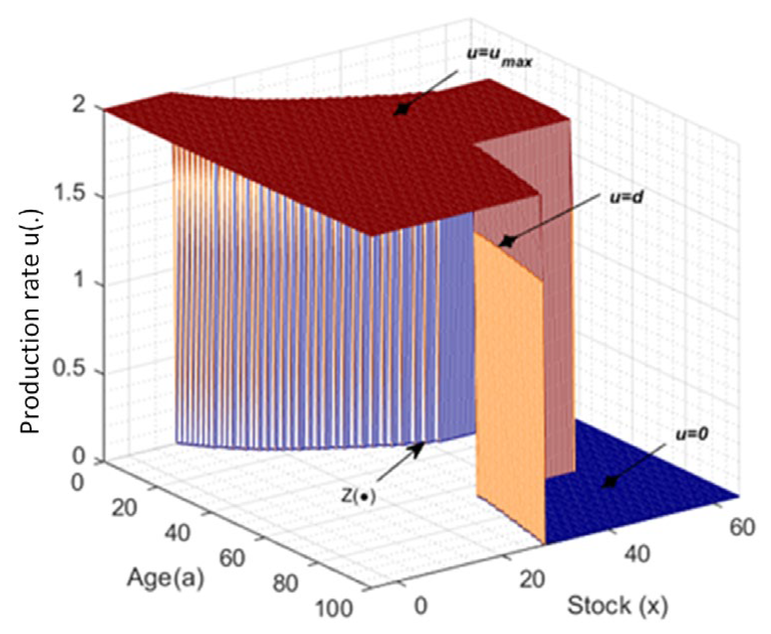
In Figure 4, the production rate of the manufacturing system is illustrated as a function of both the stock level x ( . ) and the age of the production machine a ( . ) , directly influencing emissions e ( . ) during the operational mode (see Equation (3)). To better understand the interpretation of the production policy, we divide the plan into three zones: (1), (2), and (3), as illustrated in Figure 5.
Due to the GHG emissions of the production system, we notice the critical production threshold, which shows the number of products to hold in inventory to hedge against machine breakdowns and emission penalties, exceeding the limit L . We define this critical production threshold by the age and emission-dependent threshold level, Z 1 ( . ) (see Equations (18)–(20)).
Thus, the optimal production policy of the machine is given by
i f e < V : u ( x , e , 1 ) = u m a x   i f x < Z 1 ( . ) d       i f x = Z 1 ( . ) 0       i f x > Z 1 ( . )
i f V e < L : u ( x , e , 1 ) = u m a x   i f x < Z 2 ( . ) d           i f x = Z 2 ( . ) 0             i f x > Z 2 ( . )
i f e L : u ( x , e , 1 ) = u m a x   i f x < Z 3 ( . ) d             i f x = Z 3 ( . ) 0             i f x > Z 3 ( . )
The symbol V , called the voluntary emission limit, is highlighted in Figure 5 to illustrate the emission level to switch from the critical threshold Z 1 ( . ) to the lower boundary of the critical threshold Z 2 . .   L is the emission standard limit to switch from the upper boundary of the critical threshold Z 2 ( . ) to the critical threshold Z 3 ( . ) . Thus, the obtained optimal production control policy follows distinct guidelines across three zones:
  • The production must be halted ( u . = 0 ) if the current inventory level exceeds the critical threshold Z i ;
  • The production rate must be adjusted to the value of the demand rate when the current inventory level matches the critical Z i ;
  • The production rate must be adjusted to its maximum value u m a x if the current inventory is below the critical threshold Z i .
We observe that after the emission limit L , the threshold level Z ( . ) gradually decreases, as the penalty for emissions exceeding L is relatively more costly than the shortage. It therefore pays off for decision-makers to give priority to environmental requirements. The repair activity of the machine after the occurrence of a failure, even if minimal, does not prevent the deterioration of the machine. Therefore, after a certain age, it will be difficult to satisfy the demand, or even more challenging. At the same time, we will observe a strong growth in the emissions level e t . The PM policy therefore defines when to apply the PM action, considering the threshold level x t required to satisfy the demand d . Solving the problem of optimizing the system under consideration will also involve determining the threshold necessary to restore it in order to improve its reliability   q 12 and reset its emission index θ .
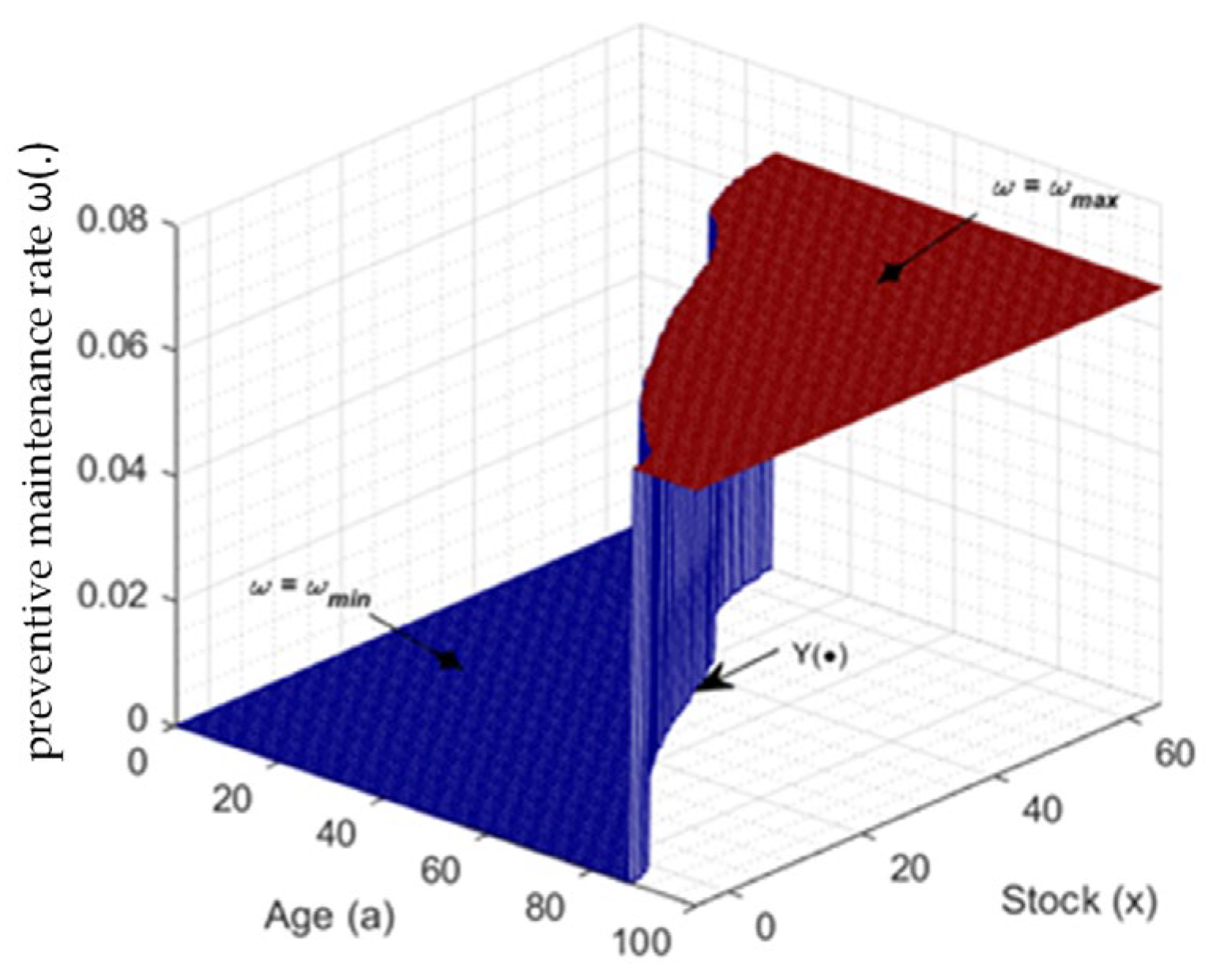
The optimal PM policy ω ( · ) , illustrated by Figure 6, indicates the PM rate, based on the inventory level x ( t ) , age a ( t ) of the machine, and emission level e ( t ) , with the maximum value ω m a x if the machine is scheduled for a PM action, and the minimum value ω m i n if the action is not recommended.
The optimal PM policy is characterized by a bang-bang control structure described as follows:
ω x , a , 3 = ω m a x   i f   x t > Y . ω m i n ,   o t h e r w i s e
where Y ( · ) is the inventory and age (emissions)-dependent function that gives the threshold level at which it is necessary to switch the PM rate from ω m i n to ω m a x . To gain a clearer understanding of the policy and in comparison with the work of Ben-Salem et al. [27], who proposed two perfectly rectangular decision zones due to the fixed nature of their critical thresholds, we have divided the plan into three zones: A, B, and C (see Figure 7).
Zone A: The machine is at a low age with minimal deterioration; the PM activity is not recommended. The machine is still in its youthful period in this zone, capable of meeting demand with infrequent failures and reduced pollution. Hence, the decision variable, ω ( · ) , is set to the minimum value, ω m i n .
Zone B: Here, the deterioration effect of the machine is more pronounced on its reliability and emission index. Due to the ageing of the machine, the emission limit imposed by the legislation will be exceeded prematurely. The cost of exceeding the emission limit is very penalizing, so the policy that recommends the machine be rushed for PM is well justified. This explains why the PM rate ω ( · ) is set to the maximum value.
Zone C: For a more precise illustration of the optimal PM policy, we present the threshold levels of production and PM policies defined by Z . , Y ( . ) . This zone is the intersection between the production and the PM threshold. We refer to the feasible zone as the area where the manufacturing system operates. This zone defines the machine’s age, the emission level, and the necessary threshold level, which indicates when the machine should be sent to the PM. Thus, the new optimal PM policy can be written as follows:
ω x , a , 3 = ω m a x   i f   x t , a t Z o n e   C ω m i n ,   o t h e r w i s e
with C = A B being defined by the state variables ( x ( t ) , a ( t ) ) .
The next section will validate the proposed model and the obtained joint optimal policy structures through a sensitivity analysis.

5. Sensitivity Analysis

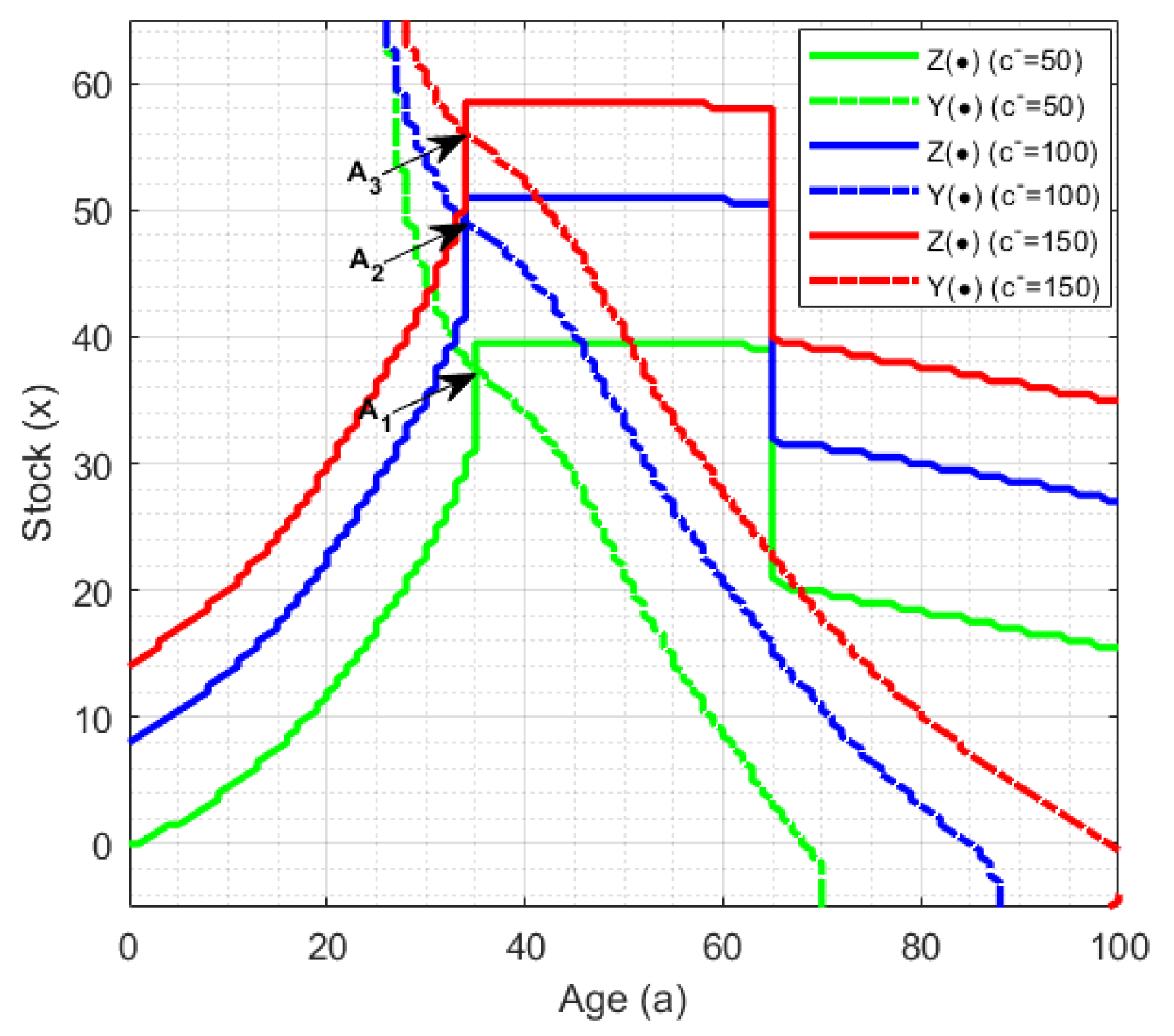
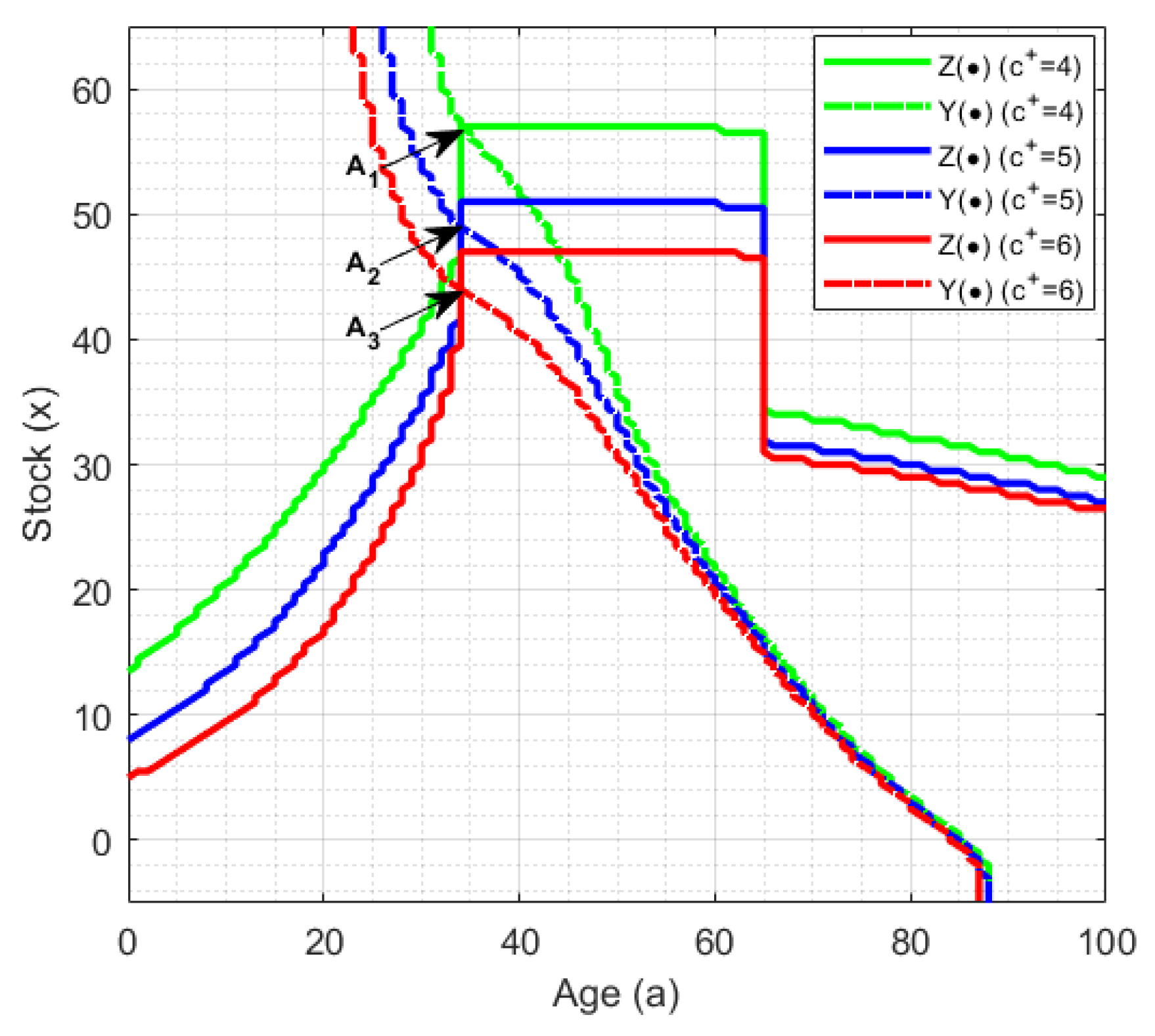
To validate the obtained control policy structure, as expressed by Equations (18)–(22), an extensive sensitivity analysis is conducted. This involves varying several selected system and cost parameters and analyzing the behaviour of the critical production thresholds Z i i = 1 , 2 , 3 , as well as the replacement zone characterized by threshold A. Three case levels are considered, representing the low, medium, and high values of the selected parameters, which include shortage, inventory, emission, and PM costs, in addition to the adjustment parameter of the emission index. Notably, the symbols A 1 , A 2 , and A 3 denote the intersection thresholds at which replacement is first recommended for the low, medium, and high case levels, respectively. The analyses were performed utilizing the numerical example presented in the previous section as a base for the study (basic case).

5.1. Shortage Cost

Figure 8 illustrates the results for three distinct values of backlog cost c = ( 50 , 100 , 150 ). It shows that when c increases, the control policy recommends increasing the production thresholds Z to reduce the risk of shortages during periods of machine breakdowns. With larger values of Z , the system results in more emissions, and the machine will deteriorate faster, leading to an increase in the feasible zone C. As a result, the PM of the machine is recommended earlier, namely a A 3 < a A 2 < a A 1 .
This result indicates that higher backlog costs incentivize maintaining higher inventory levels to buffer against potential disruptions, consequently accelerating machine wear and increasing emissions. The practical implication is that companies with high backlog costs might prioritize frequent maintenance to avoid downtime, balancing operational efficiency with environmental impact.

5.2. Inventory Cost

Figure 9 illustrates the results for three distinct values of inventory cost c + = ( 4 , 5 , 6 ). It shows that when c + increases, the policy recommends decreasing the optimal production thresholds Z to limit additional storage costs. The machine must then produce fewer parts at maximum capacity, a situation that leads to less emissions and less deterioration. Consequently, the PM of the machine is less recommended, namely a A 1 < a A 2 < a A 3 , and the feasible zone C is decreased.
This result suggests that higher inventory costs drive a strategy focused on minimizing storage, thus reducing production rates and emissions. For companies with significant inventory costs, this approach supports sustainable manufacturing practices by lowering emissions and extending machine life.

5.3. Emission Cost

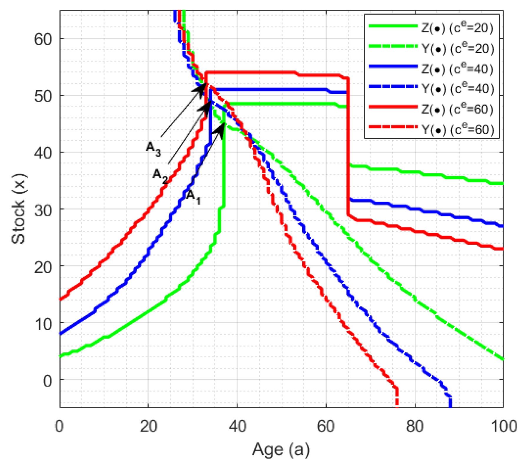
Figure 10 illustrates the results for three distinct values of emission cost c e = ( 20 , 40 , 60 ). It shows that when c e increase, PM is more recommended (i.e., a A 3 < a A 2 < a A 1 ), as the emission index is delineated as a function of the machine’s age (see Equation (3)). In addition, to avoid the excessive costs associated with significant emissions surpassing the emission limit L, the policy recommends reducing the value of V. This explains the increase in the critical production thresholds Z 1 and Z 2 and the decrease in Z 3 . These circumstances result in reduced emissions and an increased feasible zone C.
This result highlights the impact of emission costs on maintenance and production strategies. As the emission penalties rise, companies are more likely to perform PM and adjust production rates to stay within environmental limits, thereby supporting regulatory compliance and sustainability goals.

5.4. PM Cost

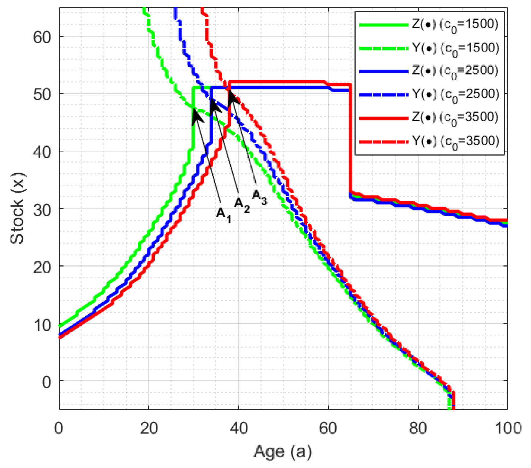
Figure 11 illustrates the results for three distinct values of PM cost c o = ( 1500 , 2500 , 3500 ). It shows that when c o increases, PM is less recommended (i.e., a A 1 < a A 2 < a A 3 ), decreasing the feasible zone C, while favouring the strategy of prolonging the machine’s operational lifespan as much as possible. With respect to the production, as c o increases, the thresholds Z increase to deal with a higher risk of breakdowns.
This result indicates that higher maintenance costs lead to a preference for less frequent maintenance, extending machine life and reducing operational disruptions. Companies with significant PM costs might prioritize strategic production planning to mitigate breakdown risks.

5.5. Adjustment Parameter of Emission Index

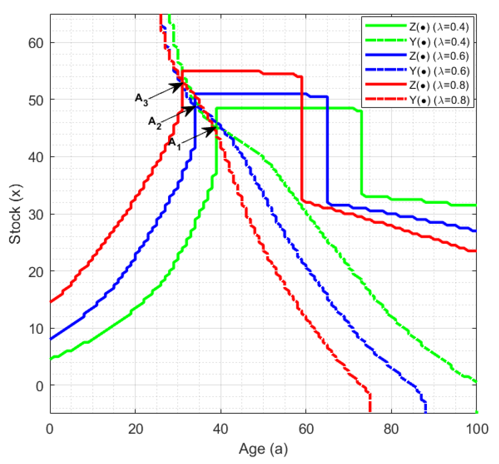
Figure 12 illustrates the results for three distinct values of the emission index λ = ( 0.4 , 0.6 , 0.8 ). It shows that when λ increases, the PM of the machine is more recommended (i.e., a A 3 < a A 2 < a A 1 ), preventing the standard emissions limit from being reached quickly. In addition, to avoid the excessive costs associated with significant emissions surpassing the emission limit L, the policy recommends increasing the critical production thresholds Z 1 and Z 2 and decreasing Z 3 . This results in an increased feasible zone C.
This result demonstrates how the emission index influences maintenance and production decisions. Higher emission indices prompt more frequent maintenance to avoid exceeding emission limits, aligning with environmental sustainability objectives.
In the next section, we conduct a comparative study to highlight the economic advantage of our optimal control policy over the one adapted from the literature.

6. Comparative Study

This section aims to assess the economic advantage of the developed optimal control policy, referred to as policy-I, compared to that used in the most closely related work found in the literature, which we refer to as policy-II. Unlike our optimal policy-I, policy-II, introduced by [27], was formulated relying on literature-based insights and common sense, while overlooking the dynamic nature of production machine ageing, which continuously influences emission rates and, consequently, the production process. Adapted to our specific context for comparison purposes, it is characterized by two fixed production thresholds Z 1 B S and Z 2 B S , a constant recommended age for PM A B S , and a voluntary emission limit V B S for adjusting the production threshold. Policy-II, given by Equations (23)–(25), can be viewed as a simplified version of our proposed one, with approximate and fewer control parameters.
We proceed to conduct a comparative analysis between policy-I and policy-II by varying the parameter of backlog cost c , inventory cost c + , emission cost c e , and PM cost c o , as well as the adjustment parameter of the emission index λ . As baseline data for the comparison, we take c + = 2 , c = 150 , c e = 40 , θ 0 = 2 , q 1 = 0.005 , q 2 = 0.0075 , q 21 = 1 / 6 , q 31 = 1 / 12 , u m a x = 2 , d = 1.5 , c r = 25 , c 0 = 2500 , ω m i n = 10 6 , and ω m a x = 1 / 15 . We consider the economic performance (the total incurred cost given by the value function) of our policy-I compared to that of policy-II.
i f e V B S : u ( x , e ) = u m a x i f x < Z 1 B S d             i f x = Z 1 B S 0             i f x > Z 1 B S
i f e > V B S : u ( x , e ) = u m a x i f x < Z 2 B S d             i f x = Z 2 B S 0           i f x > Z 2 B S
ω ( ) = 1 i f a A B S a n d x Z 2 B S 0 o t h e r w i s e
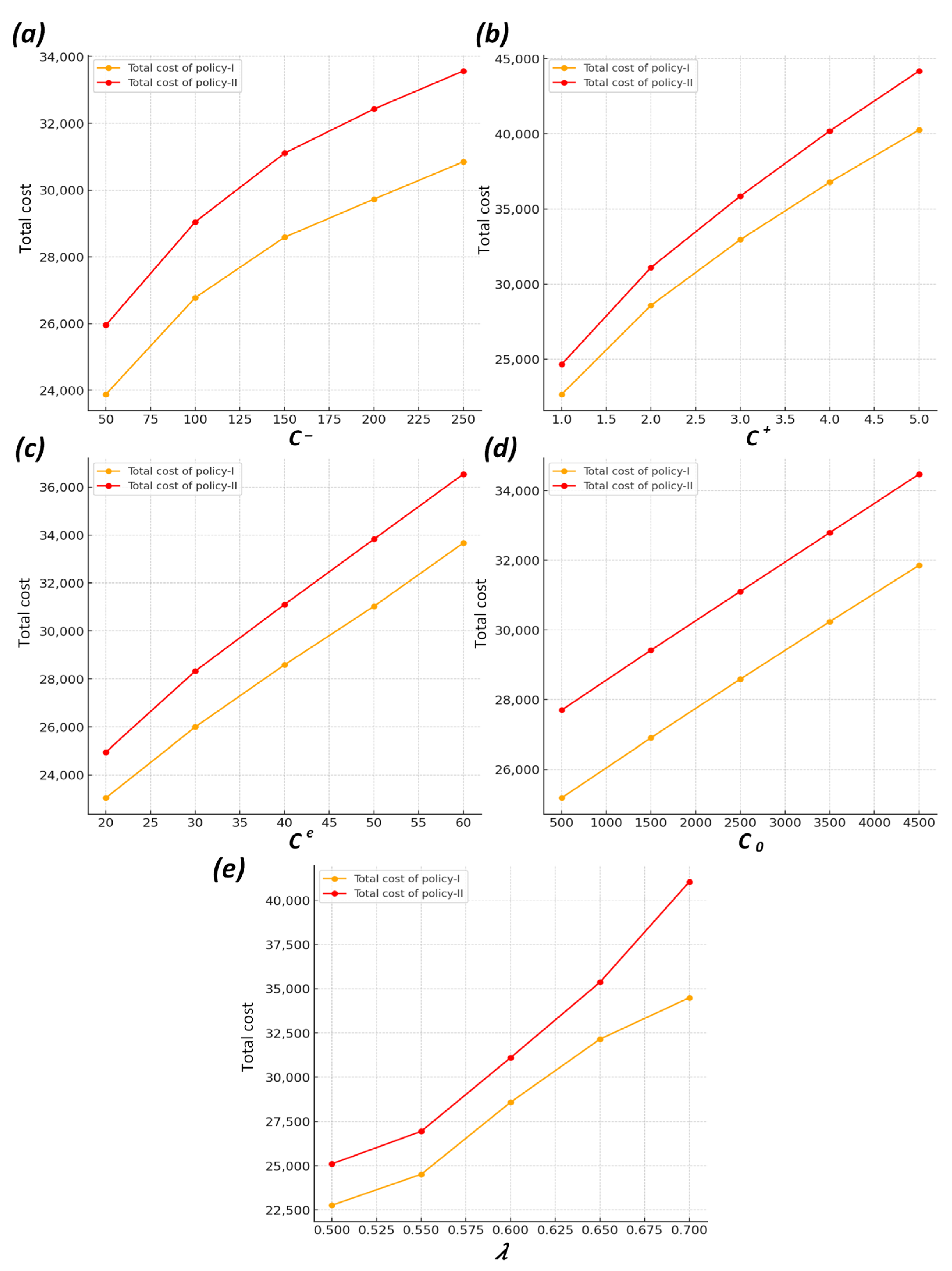
The comparison results, depicted in Figure 13, are indicative of the economic performance of policy-I and policy-II across varying system configurations. Each subfigure represents a scenario with different system parameters, providing insights into the robustness of the proposed policy. The obtained results show that the total cost of policy-I remains lower than that of policy-II, confirming the economic advantage of our proposal. Indeed, since production activity directly affects machine ageing, deterioration over time, and emissions released into the environment, it is crucial to consider all these indicators in the production planning and control process. Policy-I derives an advantage from its inherently flexible structure, characterized by a greater number of control parameters, using more thresholds to monitor inventory levels, emission volumes, and machine age. This enables policy-I to be more responsive to system state changes over time, ensuring multiple levels of decision-making. With a better control of inventory, emissions, and machine age, policy-I achieves superior production pace and preventive maintenance control, thus reducing costs related to inventory, shortages, emissions, and preventive maintenance more effectively than policy-II, which relies on fewer control parameters.
The effects of varying specific system parameters are examined to provide a comprehensive analysis of the comparative results presented in Figure 13. The following details highlight the performance differences between policy-I and policy-II under various conditions:
  • Backlog cost ( c ) (see Figure 13a): As c increases, policy-I demonstrates a consistently lower total cost compared to policy-II. Its flexibility and responsiveness allow the adjustment of the security inventory level according to the state of the system and better planning of preventive interventions, thus reducing costly failure stoppages and delays.
  • Inventory cost ( c + ) (see Figure 13b): With rising c + , policy-I shows a cost advantage, underscoring its efficiency in inventory management. Policy-I’s flexible thresholds allow for better adjustment of stock levels, thereby minimizing unnecessary inventory holding costs more effectively than policy-II.
  • Emission cost ( c e ) (see Figure 13c): The increasing c e highlights the environmental efficiency of policy-I. It proactively adjusts production to minimize emissions, effectively reducing emission-related costs more significantly than policy-II. Policy-I’s flexibility in adjusting thresholds related to emissions ensures better compliance with environmental regulations.
  • PM cost ( c o ) (see Figure 13d): The sensitivity to c o illustrates that policy-I maintains lower operational costs despite higher maintenance expenses. This is due to its capacity for effectively monitoring machine age based on failure rates and the finished products’ inventory level, thereby generating optimal costs, including preventive maintenance costs.
  • Adjustment of emission index ( λ ) (see Figure 13e): As λ increases, indicating a more stringent regulatory environment, policy-I adapts by further optimizing the trade-off between production throughput and emissions control. This flexibility allows policy-I to make more efficient decisions regarding finished product inventory size and preventive maintenance based on the evolution of emission volumes.
Our comparative study confirms the economic advantage of using the developed optimal control policy-I to manage deteriorating manufacturing systems that produce GHG emissions and operate within dynamic and stochastic environments. This positions policy-I as a superior choice for sustainable manufacturing operations.

7. Managerial Implementation

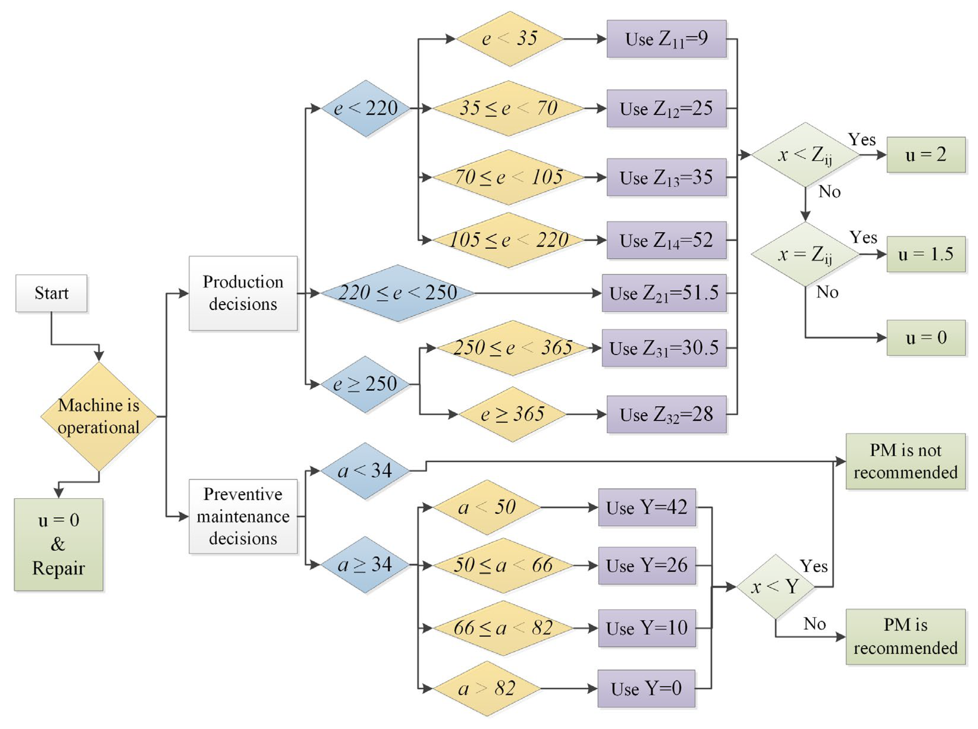
Ensuring the effective implementation of the developed control policy in business operations relies on maintaining comprehensive information about the state of the manufacturing system. This is made possible through integrating Industry 4.0 technologies, which facilitate the automatic and instantaneous collection of critical data. These technologies are essential for monitoring fundamental system elements, such as operational status, equipment age, stock levels, and GHG emission levels. The process is further supported by a logical implementation diagram, shown in Figure 14, which aids in decision-making. Our approach includes a detailed, step-by-step guide that leverages real-time data to trigger alerts when critical thresholds are reached, thus optimizing production rates and preventive maintenance schedules in response to the dynamically changing conditions of the manufacturing environment.
Our proposal establishes two controls: the production rate for safety stock building and the dispatch rate for PM activities. Given the operational status of the machine and its anticipation of the next breakdown with a stock level ( x ) , an emission level e , and an age ( a ) , the production rate can be easily defined in three stages. The first one is to build the safety stock to avoid the unavailability of finished products due to breakdowns and repairs. The second one is to decide when to decrease this stock according to the voluntary limit of emissions, and the last one is to indicate when to decrease the safety stock again when the excess cost of emissions becomes very penalizing. These stages are represented in intervals and delimited into zones, as follows: e < V , V e < L , and e L (see Equations (18)–(20)). They are designated as zone 1, zone 2, and zone 3, respectively (see Figure 5). The PM dispatch rate can be easily defined as the threshold age at which the manufacturer initiates PM on the machine, along with the buffer stock level necessary to mitigate non-availability during this activity. This level, denoted by the interval a A * , is delineated by the feasibility zone C (see Figure 7). However, from a practical perspective, implementing the critical thresholds in an industrial context is challenging. The obtained optimal structure of control policies shows that these critical thresholds, defined by Z i . , i = 1 , 2 , 3 (see Equations (18)–(20)) and Y . (see Equation (21)), are dependent on the ageing of the production machine and the cumulative volume of emissions, both of which are inherently linked to the production process. This complexity raises pertinent questions, such as determining the appropriate number of levels for the control parameter Y . and for each of the parameters Z i , which are constrained within zones 1, 2, and 3. Consequently, we determined a target value for these thresholds to obtain the best approximation of the theoretical optimal control policy. To do so, we proceeded by splitting the zones with varying critical thresholds into equal parts. We subdivided zones 1 and 3 ( e < V et e L , respectively) of our policy defined by the critical threshold Z 1 · and Z 3 · , respectively. Concerning zone 2 ( V e < L ), we took the minimum of the critical threshold Z 2 · . The control policy to be implemented, presented in Figure 14, is a good approximation of the optimal policy. Offline experiments were conducted to determine the most effective approximation, resulting in a 0.75% cost difference compared to the optimal solution. The results obtained from the numerical values, which are to be used in decision-making to facilitate the implementation of our policy, are summarized as follows: E 1 = 35 , E 2 = 70 , E 3 = 105 , V = 220 , L = 250 , E 4 = 365 , A = 34 , A 1 = 50 , A 2 = 66 , A 3 = 82 , Z 11 = 9 , Z 12 = 25 , Z 13 = 35 , Z 14 = 52 , Z 2 = 51.5 , Z 31 = 30.5 , Z 32 = 28 , Y 1 = 42 , Y 2 = 26 , Y 3 = 10 , and Y 4 = 0 . This proposal empowers managers to dynamically adjust production rates to build safety stock and scale back as needed, meeting environmental standards and operational demands. Setting predefined thresholds ensures timely adjustments in production and PM, reduces machine wear, and avoids penalties for exceeding emission limits.

8. Conclusions

In this paper, we jointly determined the optimal production and preventive maintenance policies of a manufacturing system subject to deterioration, with control over environmentally harmful greenhouse gas (GHG) emissions. For the modelling and development of the optimal policy, the optimality conditions of the HJB-type equations were determined using a stochastic dynamic programming approach. Such equations were subsequently solved numerically to characterize the optimal production policy structure that minimizes the total cost. The results showed that this combined policy relies on both the emission level and the system’s age and is defined as an environmental hedging point policy (EHPP). A sensitivity analysis was conducted, showing the impact of varying several parameters on the obtained policies in order to validate the proposed model. We continued with a comparative study to position our proposal in relation to the literature. With the lack of an existing optimal control policy, the obtained results position our work as a significant contribution to the research axis of controlling manufacturing systems under the control of GHG emissions. Finally, we outlined a managerial implementation of the proposed policy to facilitate the manufacturing system control by decision-makers.
Possible extensions of this work could integrate other environmental aspects into the model, such as reverse logistics for manufacturing/remanufacturing systems. They could expand the model to include other pollutants, such as dust and slags, providing a more comprehensive approach to managing environmental sustainability in industrial operations. Furthermore, future research could better reflect the reality of deteriorating manufacturing systems by integrating product quality as a performance metric while leveraging predictive maintenance strategies to enhance operational optimization and overall system performance [36,37,38].

Author Contributions

All authors contributed to this study’s conception and modeling. The development of optimality conditions, data collection, and simulation was performed by A.G., J.-P.K. and A.L.K.T. The first draft of the manuscript was written by A.L.K.T., A.G. and J.-P.K., while M.A. worked on the subsequent versions until the final version. All authors have read and agreed to the published version of the manuscript.

Funding

This research has been supported by the Natural Sciences and Engineering Research Council of Canada (NSERC) under grant numbers: RGPIN 2018-05292 and RGPIN-2020-05826.

Institutional Review Board Statement

Not applicable.

Informed Consent Statement

Not applicable.

Data Availability Statement

No new data were created. All the data used are presented in the manuscript.

Conflicts of Interest

The authors declare no conflicts of interest.

Abbreviations

Notations
x ( · ) inventory level of products (product);
Z ( · ) critical finished products stock level (product);
a ( · ) age of the machine according to its production rate (product);
e ( · ) emission level of the manufacturing system (emission volume);
θ ( . ) emission index (emission volume per product);
u ( · ) production rate of the manufacturing system (product per time unit);
u m a x maximal production rate of the manufacturing system (product per time unit);
d customer demand rate (product per time unit);
q α β transition rate from mode α to mode β;
ξ ( t ) stochastic process;
ρ discount rate;
c + inventory unit cost of finished products ($ per product per time unit);
c backlog unit cost ($ per product per time unit);
c r instantaneous repair cost ($ per action);
c 0 preventive maintenance cost ($ per action);
Lstandard emission limit (emission volume);
c e penalty unit cost for emissions exceeding L (USD per emission unit per time unit);
π vector of limiting probabilities;
g ( · ) instantaneous cost function (USD per time unit);
J ( · ) total cost function;
v ( · ) value function.

Appendix A

While HJB equations typically lead to solutions that are difficult to attain, Boukas and Haurie [39] successfully approximated a solution using numerical methods inspired by the approach of Kushner and Dupuis [35]. This approach allows solving the HJB equations numerically by approximating v x , a , ξ by a function v h x , a , ξ and first-order partial derivatives of the value function by finite differences involving discretization steps. It has also been used in several works, such as [13]. For our problem, we discretized on the stock of finished products x and the age of the machine a in order to obtain N x and N a points as in the following equation:
N x = x m a x x m i n h x + 1 ; N a = a m a x a m i n h a + 1
The partial derivative approximation of the finite difference value function v x , a , ξ is given as follows:
v x , a ,   ξ x = v h x + h x , a , ξ v h x , a , ξ h x i f x ˙ 0 v h x , a ,   ξ v h x h x , a ,   ξ h x   i f x ˙ < 0  
v x ,   a ,   ξ a = v h x , a + h a , ξ v h x , a , ξ h a
Substituting Equations (A2) and (A3) into Equation (16) and after simplification, we obtain the numerical version of the Hamilton–Jacobi–Bellman (HJB) Equations (A4)–(A6).
v h x , a ,   1 = m i n u , ω Γ 1 ρ + u d h x + k u h a q 11 . c + x + + c x + c e m a x 0 , e L + u d h x v h x + h x , a , 1 I + + v h x h x , a , 1 I + k u h a v h x , a + h a , 1 + q 12 v h x , φ a 2 ,   2 + ω v h x , φ a 3 , 3  
v h x ,   a , 2 = 1 ρ + d h x q 22 c + x + + c x + c r + d h x v h x h x , a , 2 + q 21 v h x , φ a 1 ,   1
v h x ,   a , 3 = 1 ρ + d h x q 33 c + x + + c x + c o q 31 + d h x v h x h x , a , 3 + q 31 v h x , φ a 1 ,   1
with I + = I n d u d 0 , I = I n d u d < 0 , q 11 = q 12 ω , and q 22 = q 21 .
Equations (A4)–(A6) represent the dynamic programming formulation for a continuous-time decision process characterized by discrete states persisting over an indefinite time horizon. To numerically solve HJB Equations (A4)–(A6), certain boundary conditions, denoted by the computational domain D, are needed.

References

  1. Ripple, W.J.; Wolf, C.; Gregg, J.W.; Rockström, J.; Newsome, T.M.; Law, B.E.; Marques, L.; Lenton, T.M.; Xu, C.; Huq, S.; et al. The 2023 state of the climate report: Entering uncharted territory. Bioscience 2023, 73, 841–850. [Google Scholar] [CrossRef]
  2. Karlina, A.I.; Karlina, Y.I.; Gladkikh, V.A. Analysis of Experience in the Use of Micro- and Nanoadditives from Silicon Production Waste in Concrete Technologies. Minerals 2023, 13, 1525. [Google Scholar] [CrossRef]
  3. Benjaafar, S.; Li, Y.; Daskin, M. Carbon Footprint and the Management of Supply Chains: Insights From Simple Models. IEEE Trans. Autom. Sci. Eng. 2013, 10, 99–116. [Google Scholar] [CrossRef]
  4. LEE, W.; YIK, F. Regulatory and voluntary approaches for enhancing building energy efficiency. Prog. Energy Combust. Sci. 2004, 30, 477–499. [Google Scholar] [CrossRef]
  5. Brouhle, K.; Griffiths, C.; Wolverton, A. Evaluating the role of EPA policy levers: An examination of a voluntary program and regulatory threat in the metal-finishing industry. J. Environ. Econ. Manag. 2009, 57, 166–181. [Google Scholar] [CrossRef]
  6. Rosen, M.A.; Kishawy, H.A. Sustainable Manufacturing and Design: Concepts, Practices and Needs. Sustainability 2012, 4, 154–174. [Google Scholar] [CrossRef]
  7. Hao, X.; Demir, E. Artificial intelligence in supply chain decision-making: An environmental, social, and governance triggering and technological inhibiting protocol. J. Model. Manag. 2024, 19, 605–629. [Google Scholar] [CrossRef]
  8. Cheng, K.; Srai, J.S. Special issue on sustainable manufacturing and the key enabling technologies. Proc. Inst. Mech. Eng. Part B J. Eng. Manuf. 2012, 226, 1603. [Google Scholar] [CrossRef]
  9. Setchi, R.; Maropoulos, P. Editorial for the Special Issue on Sustainable Design and Manufacturing. Proc. Inst. Mech. Eng. Part B J. Eng. Manuf. 2018, 232, 1689. [Google Scholar] [CrossRef]
  10. Bouslikhane, S.; Hajej, Z.; Rezg, N. An optimal mathematical modeling for manufacturing/remanufacturing problem under carbon emission constraint. In Proceedings of the 2017 7th International Conference on Modeling, Simulation, and Applied Optimization (ICMSAO), Sharjah, United Arab Emirates, 4–6 April 2017; IEEE: New York, NY, USA, 2017; pp. 1–5. [Google Scholar]
  11. Akella, R.; Kumar, P. Optimal control of production rate in a failure prone manufacturing system. IEEE Trans. Automat. Contr. 1986, 31, 116–126. [Google Scholar] [CrossRef]
  12. Yang, J.; Yan, H.; Taksar, M.I. Optimal production and setup scheduling: A one-machine, two-product system. Ann. Oper. Res. 2000, 98, 291–311. [Google Scholar] [CrossRef]
  13. Ouaret, S.; Kenné, J.-P.; Gharbi, A.; Polotski, V. Age-dependent production and replacement strategies in failure-prone manufacturing systems. Proc. Inst. Mech. Eng. Part B J. Eng. Manuf. 2017, 231, 540–554. [Google Scholar] [CrossRef]
  14. Diop, I.; Nadeau, S.; Emami-Mehrgani, B. A Mathematical Model: A Flexible Manufacturing System, Prone to Error, Making Two Products Each with Stochastic Demand Schedules. Am. J. Ind. Bus. Manag. 2019, 9, 139–168. [Google Scholar] [CrossRef]
  15. Ouaret, S. Production control problem with semi-Markov jump under stochastic demands and deteriorating inventories. Appl. Math. Model. 2022, 107, 85–102. [Google Scholar] [CrossRef]
  16. Aghdam, S.S.; Fattahi, P.; Hosseini, S.M.H.; Babaeimorad, S.; Sana, S.S. Joint optimisation of the maintenance and buffer stock policies considering back orders. Int. J. Syst. Sci. Oper. Logist. 2023, 10, 2169054. [Google Scholar] [CrossRef]
  17. Gong, X.; Zhou, S.X. Optimal Production Planning with Emissions Trading. Oper. Res. 2013, 61, 908–924. [Google Scholar] [CrossRef]
  18. He, P.; Zhang, W.; Xu, X.; Bian, Y. Production lot-sizing and carbon emissions under cap-and-trade and carbon tax regulations. J. Clean. Prod. 2015, 103, 241–248. [Google Scholar] [CrossRef]
  19. Zhou, M.; Pan, Y.; Chen, Z.; Chen, X. Environmental resource planning under cap-and-trade: Models for optimization. J. Clean. Prod. 2016, 112, 1582–1590. [Google Scholar] [CrossRef]
  20. Xu, X.; Xu, X.; He, P. Joint production and pricing decisions for multiple products with cap-and-trade and carbon tax regulations. J. Clean. Prod. 2016, 112, 4093–4106. [Google Scholar] [CrossRef]
  21. Pan, X.; Li, S. Optimal control of a stochastic production–inventory system under deteriorating items and environmental constraints. Int. J. Prod. Res. 2015, 53, 607–628. [Google Scholar] [CrossRef]
  22. Kumari, M.; Kanti De, P.; Narang, P.; Shah, N.H. Integrated optimization of inventory, replenishment, and vehicle routing for a sustainable supply chain utilizing a novel hybrid algorithm with carbon emission regulation. Expert Syst. Appl. 2023, 220, 119667. [Google Scholar] [CrossRef]
  23. Hajej, Z.; Rezg, N.; Bouslikhane, S. A Joint Production and Maintenance Optimization of Closed-Loop Production System under Carbon Emission with a Switching Subcontractor Consideration. Appl. Sci. 2019, 9, 1105. [Google Scholar] [CrossRef]
  24. Turki, S.; Rezg, N. Impact of the Quality of Returned-Used Products on the Optimal Design of a Manufacturing/Remanufacturing System under Carbon Emissions Constraints. Sustainability 2018, 10, 3197. [Google Scholar] [CrossRef]
  25. Turki, S.; Sauvey, C.; Rezg, N. Modelling and optimization of a manufacturing/remanufacturing system with storage facility under carbon cap and trade policy. J. Clean. Prod. 2018, 193, 441–458. [Google Scholar] [CrossRef]
  26. Ben-Salem, A.; Gharbi, A.; Hajji, A. An Environmental Hedging Point Policy to control production rate and emissions in unreliable manufacturing systems. Int. J. Prod. Res. 2015, 53, 435–450. [Google Scholar] [CrossRef]
  27. Ben-Salem, A.; Gharbi, A.; Hajji, A. Environmental issue in an alternative production–maintenance control for unreliable manufacturing system subject to degradation. Int. J. Adv. Manuf. Technol. 2015, 77, 383–398. [Google Scholar] [CrossRef]
  28. Afshar-Bakeshloo, M.; Bozorgi-Amiri, A.; Sajadi, S.M.; Jolai, F. A multi-objective Environmental Hedging Point Policy with customer satisfaction criteria. J. Clean. Prod. 2018, 179, 478–494. [Google Scholar] [CrossRef]
  29. Behnamfar, R.; Sajadi, S.M.; Tootoonchy, M. Developing environmental hedging point policy with variable demand: A machine learning approach. Int. J. Prod. Econ. 2022, 254, 108640. [Google Scholar] [CrossRef]
  30. McKinnon, A.; Browne, M.; Whiteing, A.; Piecyk, M. Green Logistics: Improving the Environmental Sustainability of Logistics; Kogan Page Publishers: London, UK, 2015; ISBN 0749471867. [Google Scholar]
  31. Brandenburg, M.; Hahn, G.J.; Rebs, T. Social and Environmental Dimensions of Organizations and Supply Chains; Springer: Berlin/Heidelberg, Germany, 2018. [Google Scholar]
  32. Saihi, A.; Ben-Daya, M.; As’ad, R.A. Maintenance and sustainability: A systematic review of modeling-based literature. J. Qual. Maint. Eng. 2023, 29, 155–187. [Google Scholar] [CrossRef]
  33. Psarommatis, F.; May, G.; Azamfirei, V. Envisioning maintenance 5.0: Insights from a systematic literature review of Industry 4.0 and a proposed framework. J. Manuf. Syst. 2023, 68, 376–399. [Google Scholar] [CrossRef]
  34. Cheng, G.Q.; Zhou, B.H.; Li, L. Integrated production, quality control and condition-based maintenance for imperfect production systems. Reliab. Eng. Syst. Saf. 2018, 175, 251–264. [Google Scholar] [CrossRef]
  35. Kushner, H.J.; Dupuis, P.G. Numerical Methods for Stochastic Control Problems in Continuous Time; Springer: New York, NY, USA, 1992; ISBN 1-4612-6531-2. [Google Scholar]
  36. Zhao, Y.; He, Y.; Zhou, D.; Zhang, A.; Han, X.; Li, Y.; Wang, W. Functional risk-oriented integrated preventive maintenance considering product quality loss for multistate manufacturing systems. Int. J. Prod. Res. 2021, 59, 1003–1020. [Google Scholar] [CrossRef]
  37. Han, X.; Wang, Z.; Xie, M.; He, Y.; Li, Y.; Wang, W. Remaining useful life prediction and predictive maintenance strategies for multi-state manufacturing systems considering functional dependence. Reliab. Eng. Syst. Saf. 2021, 210, 107560. [Google Scholar] [CrossRef]
  38. Li, Y.; He, Y.; Liao, R.; Zheng, X.; Dai, W. Integrated predictive maintenance approach for multistate manufacturing system considering geometric and non-geometric defects of products. Reliab. Eng. Syst. Saf. 2022, 228, 108793. [Google Scholar] [CrossRef]
  39. Boukas, E.K.; Haurie, A. Manufacturing flow control and preventing maintenance: A stochastic control approach. IEEE Trans. Automat. Contr. 1990, 35, 1024–1031. [Google Scholar] [CrossRef]
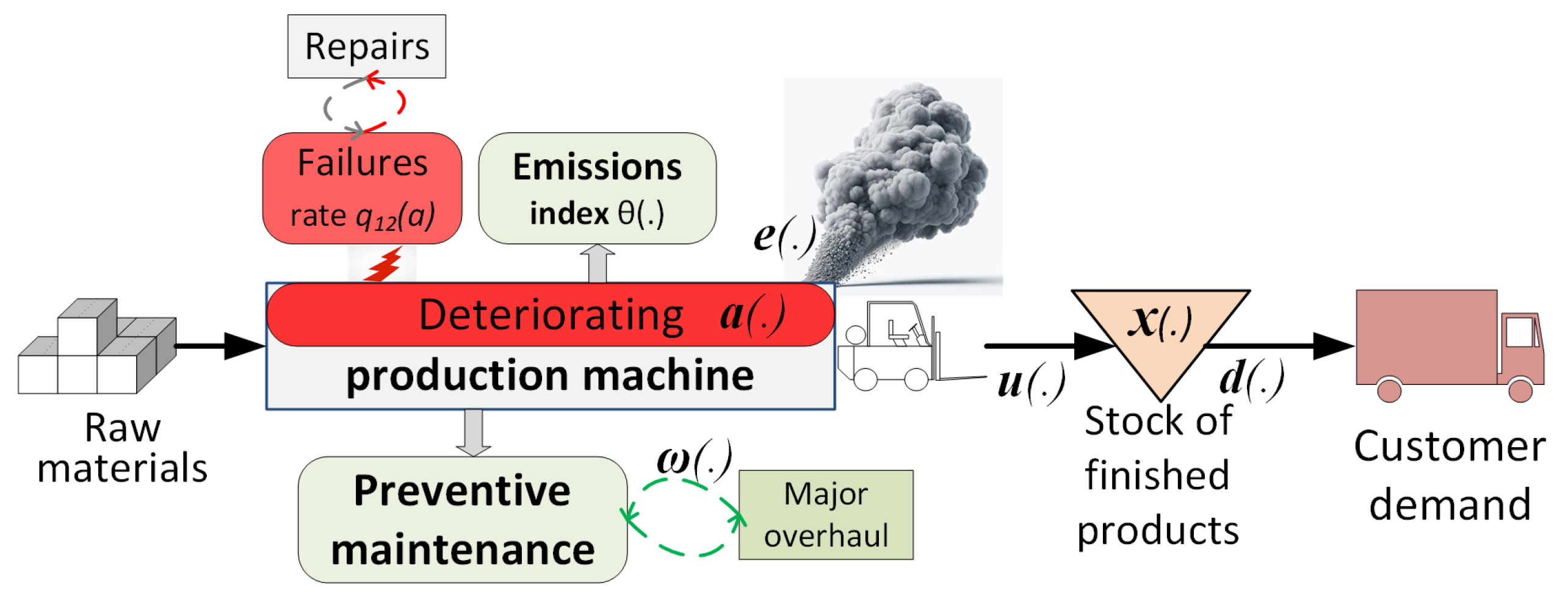
Figure 1. Overview of the studied manufacturing system.
Sustainability 16 06146 g001
Figure 2. State transition diagram.
Sustainability 16 06146 g002
Figure 3. Evolution of the failure rate (a) and emission index (b) with age.
Sustainability 16 06146 g003
Figure 4. Production policy.
Sustainability 16 06146 g004
Figure 5. Thresholds of production policy.
Sustainability 16 06146 g005
Figure 6. Preventive maintenance policy.
Sustainability 16 06146 g006
Figure 7. Threshold of production and PM policies.
Sustainability 16 06146 g007
Figure 8. Variation of c and sensitivity on Z .
Sustainability 16 06146 g008
Figure 9. Variation of c + and sensitivity analysis with respect to Z .
Sustainability 16 06146 g009
Figure 10. Variation of c e and sensitivity analysis with respect to Z .
Sustainability 16 06146 g010
Figure 11. Variation of c o and sensitivity analysis with respect to Z .
Sustainability 16 06146 g011
Figure 12. Variation of λ and sensitivity analysis with respect to Z .
Sustainability 16 06146 g012
Figure 13. System parameters’ effects on the total cost of both policy-I and policy-II.
Sustainability 16 06146 g013
Figure 14. Implementation scheme of the control policy.
Sustainability 16 06146 g014
Table 2. Data for the numerical example.
c + c c r c 0 c e u m a x d L k K 0
51002525004021.52500.80.005
K 1 K 2 k 3 θ 0 λ ρ ω m i n 1 ω m a x 1 q 21 1 q 31 1
0.00755.10−60.0220.60.01106 15 6 12
Disclaimer/Publisher’s Note: The statements, opinions and data contained in all publications are solely those of the individual author(s) and contributor(s) and not of MDPI and/or the editor(s). MDPI and/or the editor(s) disclaim responsibility for any injury to people or property resulting from any ideas, methods, instructions or products referred to in the content.