

Inter- and Intra-Driver Reaction Time Heterogeneity in Car-Following Situations

Department of Public Works, Faculty of Engineering, Ain Shams University, Cairo 11566, Egypt
Sustainability 2024, 16(14), 6182; https://doi.org/10.3390/su16146182
Submission received: 3 May 2024
/
Revised: 8 July 2024
/
Accepted: 11 July 2024
/
Published: 19 July 2024
(This article belongs to the Special Issue Road Safety and Road Infrastructure Design)
Abstract
:This study aims to examine the differences in drivers’ reaction time (RTs) while driving on horizontal curves and straight roadway segments, among different driver classes, and in different driving environments to better understand human driver behavior in typical car-following situations. Therefore, behavioral measures were extracted from naturalistic car-following trajectories to estimate the RT. The RT was estimated for two stimulus–response pairs, namely, the speed–gap and relative speed–acceleration pairs, by using the cross-classification method. The RT was estimated separately for each driver and aggregated based on location and based on driver class. The results reveal that drivers’ RTs on curves are consistently higher than their RTs on straight segments, and this difference is statistically significant. The comparison between normal drivers and aggressive drivers indicates that regardless of the location, aggressive drivers have a significantly longer RT than normal drivers, as aggressive drivers can accept closer gaps and higher relative speed. Also, cautious drivers have a longer RT compared with normal drivers; however, the difference is not significant in most cases. Furthermore, cautious and normal drivers have longer RTs on curves compared with their RTs on straight segments. Additionally, the RT on rural horizontal curves is longer than the RT on urban curves, yet the differences are insignificant.
1. Introduction
Car-following behavior modeling is essential to understanding and simulating human driver behavior and to emulating safe human driver behavior while transitioning to a fully autonomous vehicle (AV) environment and can also contribute to sustainable traffic safety, which is a pillar of sustainable transport. Accordingly, numerous studies have followed various approaches to developing car-following models by using mathematical formulations [1,2,3,4] or machine learning techniques [5,6,7]. The literature has recognized that one of the important human factors that impacts the reliability of car-following models and affects traffic dynamics microscopically and macroscopically is driver reaction time (RT) [8,9,10,11,12]. Therefore, huge research efforts have attempted the integration of RT into car-following model development [2,5,13,14,15,16,17]. In addition to car-following modeling, RT is an essential element in highway geometric design [18] and traffic signal design [19].
A driver’s RT (or reaction delay) is defined in the car-following modeling literature as the time lag of a response to its stimulus [16]. In other words, the RT is the time that elapses from the presence of a stimulus (i.e., perception) to the driver’s foot hitting the pedal (either the brake or gas pedal) (i.e., physical response) [20,21,22,23].
Although some studies have acknowledged the heterogeneous nature of driver behavior while developing car-following models [13] and the variation in driver RT due to traffic conditions changes [24], the typical RT (i.e., non-emergency RT) is implicitly assumed to be unaltered with surrounding infrastructure changes. However, previous studies have revealed that a change in the surrounding infrastructure can significantly impact driver behavior [25,26]. One of the critical changes in the surrounding infrastructure that a driver can face is the transition from driving on a straight roadway segment to a horizontal curve (HC). Generally, HCs should be designed to ensure that drivers travel across a horizontal alignment safely and conveniently. Nonetheless, drivers could experience higher visual demands during HC entry and navigation [27], in addition to higher discomfort levels that will impact their behavior [28]. Moreover, drivers on HCs will be exposed to an additional mental workload that can impact their behavior and their safety [29,30,31].
Therefore, this study aims to investigate the change in driver non-emergency RTs during typical car-following situations on HCs. To reach this goal, the following objectives should be achieved:
- Examine the differences in driver RTs while driving on straight segments and HCs (intra-driver heterogeneity).
- Investigate the differences in various driver classes (i.e., cautious, normal, and aggressive drivers) on straight segments and HCs (inter-driver heterogeneity).
- Explore the change in RT in different driving environments (i.e., urban and rural).
Intra-driver heterogeneity is defined in this study as the diversity in driver behavior or performance, specifically when it pertains to RT, among different drivers. This heterogeneity is examined among different driver groups (i.e., cautious, normal, and aggressive). On the other hand, inter-driver heterogeneity is defined here as the divergency that the same driver exhibits when driving in different contexts, such as straight segments vs. HCs and rural vs. urban areas.
The following vehicle’s location, speed, acceleration, gap, and the relative speed between the leading and the following vehicles were extracted from a total of 7483 car-following trajectories. These parameters were used as stimulus–response pairs to estimate the RT for each car-following situation by using the cross-correlation method, which is a commonly used method to estimate RT for car-following model development [16,32,33,34,35]. The RT was separately estimated for straight segments and HCs and based on various segment lengths of the car-following trajectory (i.e., 5, 8, and 10 s for the car-following trajectory, as well as the whole trajectory as one segment). Also, the RT was estimated for each driver in the dataset, and based on the driver classification reported in [26], the RT of different driver classes (i.e., cautious, normal, and aggressive drivers) were compared by using statistical testing. Furthermore, the RT change in different driving environments (i.e., urban and rural) was assessed.
2. Previous Work
Driver RT has been considered in several areas of transportation research, including but not limited to distracted driving [36,37], driver impairment [38,39], traffic safety for the aging population [40,41], reliability-based design [42,43], and cut-in behavior [44]. In addition to these areas, RT was included and investigated in different forms in several studies for emergency braking situations and forward collision warning/avoidance system development [45,46,47,48]. On the other hand, non-emergency RT is an integral component of typical car-following models. Since this study focuses mainly on RT in typical car-following situations, this section will present some examples related to car-following model development and how RT is considered in these models.
Zhou et al. proposed a recurrent neural network model to predict traffic oscillation behavior under stop-and-go conditions. To account for RT in the model, multiple behavioral measures (e.g., relative speed, following vehicle’s speed, gap, etc.) at a 0.1 s time step were prepared as inputs to the model [49]. Khodayari et al. (2012) proposed a modified neural network model to predict the following vehicle’s acceleration in car-following situations. The instantaneous RT, which was estimated based on a stimulus–response idea, was considered an input to the proposed model [5]. Also, Yao et al. considered a constant RT value for three car-following cases while investigating the interactions between connected automated vehicles and human-driven vehicles [10].
Yang and Peng (2010) proposed a stochastic car-following model that can generate nominal and erroneous driver behavior. The reaction delay was included as a source of driver error in addition to another two sources (i.e., human perceptual limitation and distraction). Although the reaction delay was acknowledged in the model by a stochastic function, roadway alignment was not considered [50]. Davis (2003) proposed a modification to the optimal velocity car-following model to incorporate driver RT. This modification eliminates the unphysical short-period oscillations of vehicle velocity due to short RT in this type of car-following model [51].
Moreover, Harth et al. (2022) incorporated the human reaction delay into a long short-term memory-based car-following model. Although the model has an input variable for HCs, the model is based on a fixed RT (one second). The model also accounts for differences between drivers, and the study compared the results with other car-following models [52]. Aghabayk et al. highlighted the significant influence that heavy vehicles can have on the car-following behavior between heavy vehicles and passenger cars including the RT. The RT was found to have its highest value when car following included two heavy vehicles; conversely, the RT with two passenger cars in a car-following situation had its lowest value. This change in RT, in addition to the variation in other measures (e.g., acceleration, space and time headway, etc.), can significantly impact [53] car-following model thresholds [54].
Zhang (2014) investigated the nature of multianticipative car following by using a multiple linear regression approach. To interpret this behavior in congested traffic conditions, the RT was investigated [33]. Xie et al. studied the heterogeneity in car-following behavior and among driver classes by analyzing various parameters, including RT. It was concluded that RT changes from one class to another based on aggressiveness and sensitivity [34]. Also, Ding et al. used RT to propose a driver identification method that models the driver’s internal stochasticity [35]. On the other hand, some studies proposed car-following decision-making models by using deep reinforcement learning or developing a multivariant modeling framework by using a coupled hidden Markov model and comparing the similarities of different driving styles based on naturalistic driving data, yet these studies indirectly considered the RT through some modeling assumptions [55,56].
Although RT is recognized as a fundamental factor in the development of car-following models, the impact of horizontal alignment change (i.e., HCs) on RT has not been explicitly examined. For example, HC was included in car-following model development, but the RT was fixed and limited to one second [52]. On the other hand, while the variability in RT was considered [5,55], the impact of HCs on the RT was not considered. Therefore, this study sheds light on the impact of the change in RT on HCs compared with straight segments across different driver classes.
3. Materials and Methods
3.1. Data Description
Naturalistic driving study (NDS) data have been identified as a reliable data source when studying driver behavior and human factors. These data record drivers’ actual behavior and performance measures while driving in different environments (e.g., rural, urban, free flow, congestion, etc.) and in various situations (e.g., car following, lane changing, driver distraction, etc.), considering all network features and infrastructure (e.g., intersections, HCs, tunnels, etc.). Therefore, this study uses an NDS dataset to compare normal driver RT on straight segments versus HCs. The NDS dataset used in this study comes from Safety Pilot Model Deployment (SPMD), which is a data collection effort under real-life conditions in Ann Arbor, Michigan, US [57,58]. The dataset was collected from host vehicles equipped with Integrated Safety Devices (ISDs). Each second, the ISD unit recorded data including position and GPS details (e.g., latitude, longitude, elevation, speed, and GPS-based data fidelity measures) and driver behavior data (e.g., braking status, speed, yaw rate, and acceleration). In addition, the dataset contains radar data collected from the ISD unit. The radar data provide information about the detected vehicle type (e.g., light vehicle, heavy vehicle, bike, pedestrian, or unclassified), status (i.e., moving and on the path), the distance from the host vehicle, and the speed relative to the object in front of the host vehicle [57,59]. This dataset has been used in several driver behavior and car-following modeling studies [56,60,61]. For more details about the dataset used in this study, readers are directed to [26,46,60,61,62].
3.2. Car-Following Period Extraction and Preparation
In order to estimate the RT for drivers, first, the NDS dataset was filtered; then, the car-following periods were identified and extracted. The main goal of this process was to ensure that the leading and following vehicles were moving and following each other in the same lane during the entire car-following period. The following steps summarize the data preparation and car-following period extraction process.
- Preparing and filtering the data:
- (a)
- We removed all invalid GPS points and invalid radar data points.
- (b)
- We removed all sensed object types, except those which were recognized as light vehicles (i.e., passenger cars). For instance, the objects that were detected as bikes, pedestrians, and heavy vehicles (i.e., trucks) were removed. This was performed as this study focuses on interactions of drivers of light vehicles and since car-following-truck behavior is different from car-following-car behavior [54,63].
- Car-following period extraction criteria were adapted from previous studies that have dealt with car-following modeling [13,64], and these criteria are summarized as follows:
- (c)
- The leading vehicle ID remained the same for 15 s at least during the car-following period.
- (d)
- The maximum range between the following and leading vehicles was 120 m to avoid free-flow conditions.
- (e)
- The maximum lateral distance between the following and leading vehicles was 2.5 m to ensure that both were in the same lane.
- (f)
- The maximum speed during the car-following period was more than 20 km/h to avoid having the entire car-following period in a stop-and-go condition.
After extracting the car-following events, the Hampel filter was applied to the behavioral measures used in this study, including the following vehicle’s speed and acceleration and the relative speed and distance between the following and leading vehicles [65,66] to remove any noise that may exist in these behavioral measures.
A total of 7483 car-following periods were extracted for all the drivers in the dataset. The minimum, average, and maximum length of these car-following periods were 15, 36.9, and 318.9 s, respectively. To facilitate the comparison between the drivers, any driver that had less than 10 car-following periods regardless of the length of the car-following periods was excluded. Accordingly, 55 drivers (out of 63 drivers) were qualified for further 180 investigations in this study. Among the extracted car-following periods, by using ArcGIS 10, 357 car-following situations were identified to occur on HCs with minimum, average, and maximum lengths of 5, 15.3, and 67.2 s, respectively. A minimum of 5 s of car-following was accepted as long as these curve-related 5 s segments were portions of a car-following period that lasted 15 s or more.
The identified 357 curve-related car-following trajectories occurred on 43 horizontal curves (including 10 curves in an urban context and 33 curves in a rural context). The average radius of the rural curves was about 900 m and 300 m for the urban curves. The car-following periods processed in this study did not have any evasive maneuvers [67], which is evident in the following summary statistics of the acceleration values:
- The average acceleration was 0.525 m/s2, and the standard deviation was 0.298 m/s2;
- The maximum acceleration was 5.13 m/s2;
- The average deceleration was −0.483 m/s2, and the standard deviation was 0.297 m/s2;
- The maximum deceleration was −6.54 m/s2.
3.3. Reaction Time Estimation
Due to the importance of driver RT estimation, several methods have been used in the literature for this purpose. For example, Gurusinghe et al. proposed a graphical method to measure the RT manually between a local minimum/maximum relative speed value and the following local minimum/maximum acceleration value [68]. This method was used by [69] to assess the impact of forward collision warning on RT. However, this method is inefficient in terms of processing and extraction time, as highlighted by [69]. Also, Ma and Andreasson introduced spectrum analyses to estimate the RT; however, this method was inefficient when dealing with narrow-band time series (e.g., relative speed), in addition to its higher difficulty level to be applied and validated in practice [21].
On the other hand, one of the most commonly used RT estimation methods that are applied to NDS for car-following behavior modeling is the cross-correlation method. This method was introduced by [16,70] and used in various car-following modeling efforts, such as [6,32,33,34,35]. Also, previous research has highlighted that this method is more efficient when dealing with relative speed (or narrow-band signals) compared with spectrum analysis [21].
To estimate the RT on HCs and straight segments, the cross-correlation method was adopted in this study. The cross-correlation method estimates the RT by identifying the time lag at which the highest cross-correlation coefficient between stimulus–response time series can be obtained. It is worth noting that the estimation of RT includes both acceleration and deceleration maneuvers. To find this time lag, the cross-correlation coefficient is calculated for several artificial time lags that are applied between both time series (i.e., stimulus–response time series). The cross-correlation method can be summarized in the following equations starting with the cross-correlation function, which can be formulated in the following form in Equation (1), and the correlation coefficient, which can be formulated as shown in Equation (2).
where Rxy (T) is the cross-correlation function, E [] is the expectation function, x(t) is the stimulus time series, y(t + T) is the response time series, and T is the time lag in seconds, while the cross-correlation coefficient is calculated according to the following equation:
where ρxy (T) is the cross-correlation coefficient, and µ and σ are the mean and standard deviation of the stimulus (x) and response (y) series. The reaction time (RT) is defined as the time lag that has the maximum correlation between the stimulus–response time series and can be described by the following equation:
Rxy (T) = E[x(t)y(t + T)]
ρxy (T) = (Rxy (T) − µx µy)/(σx σy)
RT = T|max(ρxy (T)), 0.4 ≤ T ≤ 3
As presented in Equation (3), the time lag range adopted here is between 0.4 and 3 s, since the RT has been estimated to fall within this range in previous studies [6,32,70,71,72]. For stimuli and responses, previous studies have used relative speed and the acceleration of the following vehicle as a stimulus–response pair to estimate the RT [5,6,16,32,73], while other studies have used the speed–gap (i.e., following distance) pair for the same purpose [74,75]. Therefore, both pairs (i.e., relative speed–acceleration and speed–gap) were explored in this study to capture any potential difference in the estimated RT due to the stimulus–response pair that has been used.
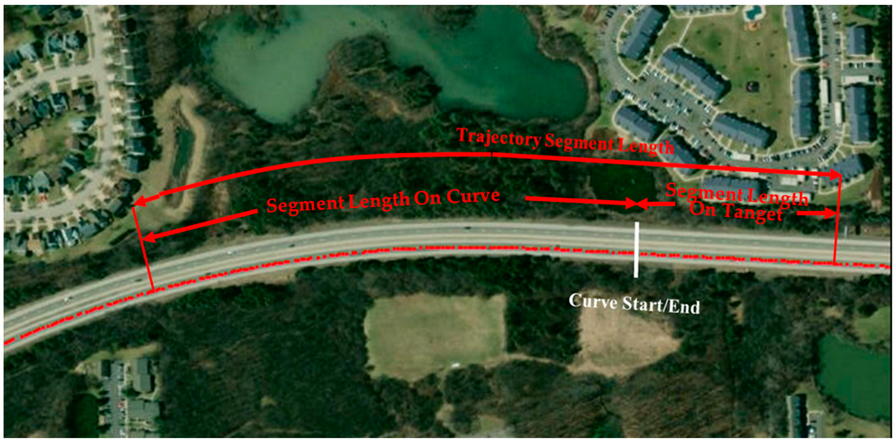
To capture the time-varying nature of RT, Ma and Qu suggested applying the cross-correlation method on smaller segments of the extracted car-following trajectory and estimating the RT for each of these smaller segments. The lengths of these segments were selected to be 5, 8, and 10 s [6]. For the purpose of this study, Ma and Qu’s method was adopted in addition to applying the cross-correlation method on the whole car-following trajectory without any segmentation. Based on this segmentation, part of the trajectory segment may fall within an HC, while the rest of the trajectory segment falls on the tangent, as shown in Figure 1. Therefore, the RT for a trajectory segment is identified as the RT on an HC if the percentage of the trajectory segment that falls within this curve is equal to or higher than a specific threshold percentage. To examine the impact of this percentage on the RT, the threshold percentage was selected to range from 100% to 30% with a 10% increment. For example, if 65% of the trajectory segment length falls within an HC and the threshold is set to 60%, then the RT estimated for this trajectory segment is considered the RT on an HC.
Furthermore, the impact of the driver class (i.e., cautious, normal, or aggressive) on RT was explored by calculating the average RT for each driver and statistically comparing the RT between driver classes. This study adopted the driver classification results that were published in [26], which used the same dataset.
Finally, the change in the RT on HCs in rural and urban areas was also examined in this study. A speed limit of 35 mph was established as the primary criterion to distinguish between urban and rural HCs. In other words, if the posted speed limit on an HC was higher than 35 mph, then it was considered a rural HC and vice versa.
4. Results
4.1. Reaction Time on HCs and Straight Segments
To investigate the difference in driver RT on HCs and straight segments, the two-sample Anderson–Darling (AD) test [76] was used. The null hypothesis was that the RT values on HCs and straight segments were from the same continuous distribution. The RT estimation in the literature uses gap–speed and relative speed–acceleration as stimulus–response pairs. To be consistent with previous work, this study estimated the RT for each pair (i.e., gap–speed and relative speed–acceleration), and the results of the RT estimation are reported in Table 1. The RT estimation was characterized by the mean, standard deviation (STD), and 85th-percentile values for both straight segments and HCs. Also, the RT was estimated for each trajectory segment length (i.e., 5, 8, and 10 s), in addition to the whole trajectory without segmentation, as shown in Table 1. Moreover, the RTs were estimated for each percentage of the car-following trajectory occurring within the HC (i.e., 30% to 100% with an increment of 10%) for each segment length as reported in the table.
For the gap–speed pair, as shown in Table 1, the RT on HCs was higher than the RT on straight segments except for the trajectory segment length of 5 s. For the 5 s segment length, although the RT on curves was slightly higher than the RT on straight segments in most of the cases, the differences between the RTs on straight segments and curves were not significant according to the AD test. For all the cases, the 85th percentile of the RT on curves was either equal to or higher than the RT on straight segments. For trajectories with a segment length of 10 s, there were significant differences between the RT on straight segments and HCs for almost all the cases at different confidence levels, as shown in Table 1. When estimating the RTs for the whole trajectory without any segmentation, there was a significant difference between the RT on straight segments and HCs at a 95% confidence level. Moreover, the 85th-percentile RT on HCs was substantially higher than the RT on straight segments, as shown in Table 1. Furthermore, there was a decrease in the RT values on straight segments when the trajectory length increased. For example, for the gap–speed pair, the mean RT was 1.73 s for the trajectory length of 10 s, while it was decreased to 1.62 s when the RT was estimated for the whole trajectory. On the other hand, for HCs, this pattern was not as consistent as noticed for straight segments. Nonetheless, the mean RT for the 5 s trajectory length was longer than the mean RT for the whole trajectory in both cases. This observation agrees with what was reported in the literature when estimating the RT for different trajectory segment lengths [6].
On the other hand, for the relative speed–acceleration pair, the estimated mean, STD, and 85th percentile of the RTs are shown in Table 1. For all the cases of the 5 s trajectory segment lengths, the estimated RTs on HCs were significantly different, at a 95% confidence level, and higher than the RTs on straight segments. Also, the 85th-percentile values for the RTs on HCs were equal to or higher than the values on straight segments. The same trend was noticed for trajectories with the 8 s segment length; however, the differences were not statistically significant. For the 10 s segment lengths, the mean RTs on HCs were either equal or higher than the RTs on straight segments for almost all the cases, except for when only 40% or 30% of the trajectory fell within the HC, as shown in Table 1. In these two cases (i.e., 40% and 30% of the trajectory were within the HC boundaries), the mean RTs on HCs were marginally shorter than the mean RTs on straight segments. Furthermore, the 85th-percentile RT values on curves were equal to or higher than the 85th-percentile RT on straight segments. For the RT that was estimated for trajectories as a whole, despite the difference being statistically insignificant, the mean RT on HCs was higher than the mean RT on straight segments, and the 85th percentiles were the same for curves and straight segments.
4.2. Reaction Time for Different Driver Classes
The differences in RT for different driver classes (i.e., cautious, normal, and aggressive) were explored in this study based on the results reported by Tawfeek and El-Basyouny [26]. According to Tawfeek and El-Basyouny [26], three different classes are identified for this dataset, including Groups 1, 2, and 3, which represent cautious, normal, and aggressive drivers, respectively. The mean RT was calculated for each of these three groups, as shown in Table 2, for both stimulus–response pairs. Moreover, the AD test was used to compare the RT between cautious and normal drivers and between normal and aggressive drivers. It is worth mentioning that the mean RTs for the driver classes were calculated on straight segments only for the 5, 8, and 10 s trajectory segment lengths. Moreover, the mean RTs for the three groups were calculated for the whole trajectory on straight segments and the whole trajectory on HCs.
As shown in Table 2, the mean RTs for aggressive drivers were consistently higher than for the other two classes (i.e., cautious and normal) for all the cases. Furthermore, the difference between the aggressive and normal driver groups was statistically significant for all the examined trajectory segment lengths at a 95% confidence level according to the AD test, except for the 10 s trajectory segment length. In this case, the difference was significant at a 90% confidence level for the gap–speed pair and at an 85% confidence level for the relative speed–acceleration pair. Moreover, the difference between these two driver groups (i.e., normal and aggressive) was statistically significant at a 95% confidence level when the whole trajectory (i.e., without segmentation) on segments is examined. On the other hand, the differences between the normal and cautious driver groups were not statistically significant, except for the case of the whole trajectory on segments for the gap–speed pair. Despite these insignificant differences, the normal driver group had higher mean RTs compared with the cautious drivers, except for the 5 and 8 s trajectory segment lengths for the relative speed–acceleration pair.
Furthermore, each driver group had longer RTs on HCs compared with straight segments. The difference in RT was statistically significant at a 95% confidence level for all the groups except for the aggressive drivers, as shown in Table 2. This finding confirms that driver RT when driving on HCs is longer than their RT when driving on straight segments regardless of the driver class.
4.3. Reaction Time on HCs in Rural and Urban Areas
The RTs aggregated based on different trajectory segment lengths (i.e., 5, 8, and 10 s) and for the whole trajectory within an HC were estimated. Table 3 summarizes the results for RTs in rural and urban areas, including mean, standard deviation, and 85th percentile for both stimulus–response pairs. As shown in the table, there were differences between the RTs in rural and urban environments; however, these differences were not statistically significant according to the AD test, except for the 10 s trajectory length for the gap–speed pair. In most cases, the RTs on HCs within the rural environment were higher than in the urban environment based on the mean and the 85th-percentile values.
5. Discussion
Based on the results presented earlier, the RT values can change based on the car-following trajectory length, the stimulus–response pairs used, roadway alignment (i.e., HCs or straight segments), driver class (i.e., cautious, normal, or aggressive), and driving environment (i.e., rural or urban). Despite these changes in RT values, the RT was noticed to be consistently longer on HCs compared with straight segments. The mean values of the RTs on HCs were up to 8% higher than the RT on straight segments, and the RT 85th-percentile values on HCs were up to 8% higher than on straight segments. This finding implies that drivers need a longer time to react to a stimulus when driving on HCs. The reason behind this longer RT on HCs may be attributed to a higher mental workload and the complex alignment of HCs compared with straight segments.
For the RT estimation parameters, the variation in RT values between different car-following trajectory lengths considering the same stimulus–response pair was considerable and statistically significant in some cases; for example, the RTs for the 5 s trajectory length and the whole trajectory for the same stimulus–response pair were statistically different. This means that the selection of the trajectory length during the estimation of RT should be handled with caution and based on the application, as the estimation parameters (e.g., car-following trajectory length) can cause significant differences between the RT values, as shown in Table 1. Also, the results show some differences in the mean RT values between the gap–speed and relative speed–acceleration pairs for the same trajectory lengths. These differences may be attributed to how sensitive each of these pairs is to driver reactions. In general, the speed–gap pair can capture the differences in RT between HCs and straight segments for longer trajectory segment lengths, such as 10 s and the entire trajectory. On the other hand, the relative speed–acceleration pair captures these differences for shorter trajectory segment lengths (i.e., 5 s). However, this relation should be investigated in more depth, and it is not within the scope of this study.
On the other hand, the mean RT on HCs insignificantly changed due to the change in the percentage of the trajectory length on curves. Nonetheless, the RT values on HCs remained higher than the RT values on straight segments for all the examined percentages. This finding shows that even if a small portion of a car-following period is on an HC, the HC (i.e., the change in the horizontal alignment) has an impact on the driver’s RT, and this impact is significant in some cases.
From a different perspective, when comparing the RTs of different driver classes (i.e., cautious, normal, and aggressive), the results show that the RT of aggressive drivers was typically longer than that of the other two groups regardless of the roadway alignment or trajectory segment lengths. This observation can be interpreted as aggressive drivers tending to delay their responses as they allow for shorter following distances and higher relative speeds. This is unlike cautious drivers, who respond to a stimulus quickly to avoid close proximity to a leading vehicle. This finding is consistent with previous research, which showed that cautious drivers have shorter RTs [69]. Also, the results show that all driver classes had consistently longer RT on HCs compared with straight segments. The differences in RT on HCs and straight segments were significant for cautious and normal drivers but insignificant for aggressive drivers.
Finally, the driving environment (i.e., urban and rural) of HCs may have an impact on RT. Despite the insignificant impact of the driving environment on RT, the estimated RTs on rural HCs were higher compared with the RT on urban HCs.
6. Conclusions
This study investigated the differences in driver RT on straight segments and HCs (i.e., intra-driver heterogeneity). The results show that there are differences between the RT estimated on HCs compared with the RT estimated on straight segments. Generally, the RT on HCs was up to 8% longer than the RT on straight segments. This study also analyzed the differences in RT among different driver classes (i.e., cautious, normal, and aggressive) on straight segments and HCs (inter-driver heterogeneity). The results reveal that the mean RT on HCs was significantly longer than the mean reaction on straight segments for all driver classes. Moreover, aggressive drivers had the longest RT compared with other driver classes. Furthermore, the study examined the change in RT in rural and urban HCs, and the results show that the RT on rural HCs was longer than the RT on urban HCs.
In summary, the main contributions of this study are as follows:
- Highlighting the difference between RT on straight segments and RT on horizontal curves (intra-driver heterogeneity). It is crucial to consider this change in RT on HCs in different aspects of transportation engineering. For example, transportation engineering professionals widely acknowledge that the RT default value is 2.5 s [18]. However, based on the 85th percentile of the RT reported in this study, the RT can exceed this standard value by 4–12% on HCs, which may lead to a potentially risky situation. Using a shorter RT than what the driver’s need is can result in a shorter braking distance, which in turn results in a shorter-than-needed stopping sight distance from a driver’s perspective. Hence, considering the findings of this study can directly contribute to sustainable safe roads that consider the variation in human driver behavior.
- Recognizing the changing nature of RTs for the same driver and from one driver to another while developing these car-following models (inter-driver heterogeneity), given the fact that RT is a fundamental component in car-following modeling.
- Leveraging the development of CAV applications, especially in the transition period when human-driven vehicles are still on the road. The estimated values in this study can be used within these CAV applications by acknowledging that the surrounding human-driven vehicles can be delayed in their response to a stimulus on HCs, which will contribute to the reliability of these applications.
On the other hand, as part of future research, the sensitivity of each of the used stimulus–response pairs to driver reactions on HCs should be investigated in more depth. Also, the change in RT due to the change in the traffic characteristics on HCs (including AADTs and peak-hour volumes) should be analyzed. The data used in this study were collected under clear weather conditions; therefore, the impact of different weather conditions on RT on HCs should be assessed in the future.
Funding
This research received no external funding.
Institutional Review Board Statement
Not applicable.
Informed Consent Statement
Not applicable.
Data Availability Statement
All the data used in this study are publicly available through the USDOT ITS Public Data Hub (https://www.its.dot.gov/data/) (accessed on 3 January 2018).
Conflicts of Interest
The author declares no conflicts of interest.
References
- Treiber, M.; Hennecke, A.; Helbing, D. Congested traffic states in empirical observations and microscopic simulations. Phys. Rev. E 2000, 62, 1805–1824. [Google Scholar] [CrossRef] [PubMed]
- Gipps, P.G. A behavioural car-following model for computer simulation. Transp. Res. Part B 1981, 15, 105–111. [Google Scholar] [CrossRef]
- Bando, M.; Hasebe, K.; Nakayama, A.; Shibata, A.; Sugiyama, Y. Dynamical model of traffic congestion and numerical simulation. Phys. Rev. E 1995, 51, 1035–1042. [Google Scholar] [CrossRef] [PubMed]
- Newell, G.F. A simplified car-following theory: A lower order model. Transp. Res. Part B Methodol. 2002, 36, 195–205. Available online: https://www.sciencedirect.com/science/article/pii/S0191261500000448 (accessed on 15 July 2022). [CrossRef]
- Khodayari, A.; Ghaffari, A.; Kazemi, R.; Braunstingl, R. A modified car-following model based on a neural network model of the human driver effects. Syst. Man Cybern. Part A Syst. Hum. IEEE Trans. 2012, 42, 1440–1449. [Google Scholar] [CrossRef]
- Ma, L.; Qu, S. A sequence to sequence learning based car-following model for multi-step predictions considering reaction delay. Transp. Res. Part C Emerg. Technol. 2020, 120, 102785. [Google Scholar] [CrossRef]
- Wang, X.; Jiang, R.; Li, L.; Lin, Y.L.; Wang, F.Y. Long memory is important: A test study on deep-learning based car-following model. Phys. A Stat. Mech. Its Appl. 2019, 514, 786–795. [Google Scholar] [CrossRef]
- Aycin, M.F.; Engineer, S.T.; Benekohal, R.F. Performance of the Generalized Car-Following Model Obtained from Macroscopic Flow Relationships in Simulating Field Data. In Proceedings of the 83rd TRB Annual Meeting, Washington, DC, USA, 11–15 January 2004. [Google Scholar]
- Treiber, M.; Kesting, A.; Helbing, D. Delays, inaccuracies and anticipation in microscopic traffic models. Phys. A Stat. Mech. Its Appl. 2006, 360, 71–88. [Google Scholar] [CrossRef]
- Yao, Z.; Xu, T.; Jiang, Y.; Hu, R. Linear stability analysis of heterogeneous traffic flow considering degradations of connected automated vehicles and reaction time. Phys. A Stat. Mech. Its Appl. 2021, 561, 125218. [Google Scholar] [CrossRef]
- Davoodi, N.; Soheili, A.R.; Hashemi, S.M. A macro-model for traffic flow with consideration of driver’s reaction time and distance. Nonlinear Dyn. 2016, 83, 1621–1628. [Google Scholar] [CrossRef]
- van Hinsbergen, C.P.I.J.; Schakel, W.J.; Knoop, V.L.; van Lint, J.W.C.; Hoogendoorn, S.P. A general framework for calibrating and comparing car-following models. Transp. A Transp. Sci. 2015, 11, 420–440. [Google Scholar] [CrossRef]
- Zhu, M.; Wang, X.; Wang, Y. Human-like autonomous car-following model with deep reinforcement learning. Transp. Res. Part C Emerg. Technol. 2018, 97, 348–368. [Google Scholar] [CrossRef]
- Zheng, L.; He, Z.; He, T. A flexible traffic stream model and its three representations of traffic flow. Transp. Res. Part C Emerg. Technol. 2017, 75, 136–167. [Google Scholar] [CrossRef]
- Wei, Y.; Avcı, C.; Liu, J.; Belezamo, B.; Aydın, N.; Li, P.T.; Zhou, X. Dynamic programming-based multi-vehicle longitudinal trajectory optimization with simplified car following models. Transp. Res. Part B Methodol. 2017, 106, 102–129. [Google Scholar] [CrossRef]
- Gazis, D.C.; Herman, R.; Rothery, R.W. Nonlinear Follow-the-Leader Models of Traffic Flow. Oper. Res. 1961, 9, 545–567. [Google Scholar] [CrossRef]
- Hamdar, S.H.; Mahmassani, H.S. From existing accident-free car-following models to colliding vehicles exploration and assessment. Transp. Res. Rec. 2008, 2088, 45–56. [Google Scholar] [CrossRef]
- AASHTO. A Policy on Geometric Design of Highways and Streets; American Association of State Highway and Transportation Officials: Washington, DC, USA, 2011; p. 942. [Google Scholar]
- Pande, A.; Wolshon, B. Traffic Engineering Handbook, 7th ed.; John Wiley and Sons Inc.: Hoboken, NJ, USA, 2016; pp. 109–148. Available online: https://app.knovel.com/web/toc.v/cid:kpTEHE0002/viewerType:toc//root_slug:viewerType%3Atoc/url_slug:root_slug%3Atraffic-engineering-handbook?kpromoter=federation (accessed on 7 July 2022).
- Ahemd, K.I. Modeling Drivers’ Acceleration and Lane Change Behaviour. Ph.D. Thesis, Massachusetts Institute of Technology, Cambridge, MA, USA, 1999. [Google Scholar]
- Ma, X.; Andréasson, I. Estimation of Driver Reaction Time from Car-Following Data. Transp. Res. Rec. J. Transp. Res. Board 2006, 1965, 130–141. [Google Scholar] [CrossRef]
- Gerlough, D.L.; Huber, M.J. Special Report 165: Traffic Flow Theory: A Monograph; Transportation Research Board, National Research Council: Washington, DC, USA, 1976; pp. 63–66. [Google Scholar]
- Lindorfer, M.; Mecklenbrauker, C.F.; Ostermayer, G. Modeling the Imperfect Driver: Incorporating Human Factors in a Microscopic Traffic Model. IEEE Trans. Intell. Transp. Syst. 2018, 19, 2856–2870. [Google Scholar] [CrossRef]
- Tawfeek, M.H.; El-Basyouny, K. Location-based analysis of car-following behavior during braking using naturalistic driving data. Can. J. Civ. Eng. 2019, 47, 498–505. [Google Scholar] [CrossRef]
- Tawfeek, M.H.; El-Basyouny, K. A context identification layer to the reasoning subsystem of context-aware driver assistance systems based on proximity to intersections. Transp. Res. Part C Emerg. Technol. 2020, 117, 102703. [Google Scholar] [CrossRef]
- Campbell, C.L.; Richard, C.M.; Graham, J. NCHRP Report 600: Human Factors Guidelines for Road Systems, 2nd ed.; Transportation Research Board of the National Academies: Washington, DC, USA, 2012. [Google Scholar]
- Awadallah, F. Theoretical analysis for horizontal curves based on actual discomfort speed. J. Transp. Eng. 2005, 131, 843–850. [Google Scholar] [CrossRef]
- Habib, K.; Gouda, M.; El-Basyouny, K. Calibrating Design Guidelines using Mental Workload and Reliability Analysis. Transp. Res. Rec. 2020, 2674, 360–369. [Google Scholar] [CrossRef]
- Messer, C.J. Methodology for Evaluating Geometric Design Consistency. Transp. Res. Rec. J. Transp. Res. Board 1980, 757, 7–14. [Google Scholar]
- Habib, K.; Tawfeek, M.H.; El-Basyouny, K. A System to Determine Advisory Speed Limits for Horizontal Curves based on Mental Workload and Available Sight Distance. Can. J. Civ. Eng. 2021, 49, 445–451. [Google Scholar] [CrossRef]
- Wang, J.; Zhang, L.; Lu, S.; Wang, Z. Developing a car-following model with consideration of driver’s behavior based on an Adaptive Neuro-Fuzzy Inference System. J. Intell. Fuzzy Syst. 2016, 30, 461–466. [Google Scholar] [CrossRef]
- Zhang, X. Empirical analysis of a generalized linear multianticipative car-following model in congested traffic conditions. J. Transp. Eng. 2014, 140, 04014018. [Google Scholar] [CrossRef]
- Xie, D.F.; Xie, D.F.; Zhu, T.L.; Li, Q. Capturing driving behavior Heterogeneity based on trajectory data. Int. J. Model. Simul. Sci. Comput. 2020, 11, 2050023. [Google Scholar] [CrossRef]
- Ding, Z.; Xu, D.; Zhao, H.; Moze, M.; Aioun, F.; Guillemard, F. Driver Identification through Multi-state Car Following Modeling. In Proceedings of the 2019 IEEE Intelligent Transportation Systems Conference (ITSC), Auckland, New Zealand, 27–30 October 2019; pp. 1580–1587. [Google Scholar] [CrossRef]
- Bellinger, D.B.; Budde, B.M.; Machida, M.; Richardson, G.B.; Berg, W.P. The effect of cellular telephone conversation and music listening on response time in braking. Transp. Res. Part F Traffic Psychol. Behav. 2009, 12, 441–451. [Google Scholar] [CrossRef]
- Saifuzzaman, M.; Zheng, Z.; Haque, M.M.; Washington, S. Revisiting the Task-Capability Interface model for incorporating human factors into car-following models. Transp. Res. Part B Methodol. 2015, 82, 1–19. [Google Scholar] [CrossRef]
- Pavlou, D.; Papadimitriou, E.; Antoniou, C.; Papantoniou, P.; Yannis, G.; Golias, J.; Papageorgiou, S.G. Comparative assessment of the behaviour of drivers with Mild Cognitive Impairment or Alzheimer’s disease in different road and traffic conditions. Transp. Res. Part F Traffic Psychol. Behav. 2017, 47, 122–131. [Google Scholar] [CrossRef]
- Yadav, A.K.; Velaga, N.R. Modelling the relationship between different Blood Alcohol Concentrations and reaction time of young and mature drivers. Transp. Res. Part F Traffic Psychol. Behav. 2019, 64, 227–245. [Google Scholar] [CrossRef]
- Gargoum, S.A.; Tawfeek, M.H.; El-Basyouny, K.; Koch, J.C. Available sight distance on existing highways: Meeting stopping sight distance requirements of an aging population. Accid. Anal. Prev. 2018, 112, 56–68. [Google Scholar] [CrossRef]
- Leversen, J.S.R.; Hopkins, B.; Sigmundsson, H. Ageing and driving: Examining the effects of visual processing demands. Transp. Res. Part F Traffic Psychol. Behav. 2013, 17, 1–4. [Google Scholar] [CrossRef]
- Wood, J.S.; Donnell, E.T. Stopping sight distance and available sight distance new model and reliability analysis comparison. Transp. Res. Rec. 2017, 2638, 1–9. [Google Scholar] [CrossRef]
- Essa, M.; Sayed, T.; Hussein, M. Multi-mode reliability-based design of horizontal curves. Accid. Anal. Prev. 2016, 93, 124–134. [Google Scholar] [CrossRef]
- Fu, R.; Li, Z.; Sun, Q.; Wang, C. Human-like car-following model for autonomous vehicles considering the cut-in behavior of other vehicles in mixed traffic. Accid. Anal. Prev. 2019, 132, 105260. [Google Scholar] [CrossRef]
- Han, H.; Kim, S.; Choi, J.; Park, H.; Yang, J.H.; Kim, J. Driver’s avoidance characteristics to hazardous situations: A driving simulator study. Transp. Res. Part F Traffic Psychol. Behav. 2021, 81, 522–539. [Google Scholar] [CrossRef]
- Tawfeek, M.H.; El-Basyouny, K. A perceptual forward collision warning model using naturalistic driving data. Can. J. Civ. Eng. 2018, 45, 899–907. [Google Scholar] [CrossRef]
- Wang, W.; Cheng, Q.; Li, C.; André, D.; Jiang, X. A cross-cultural analysis of driving behavior under critical situations: A driving simulator study. Transp. Res. Part F Traffic Psychol. Behav. 2019, 62, 483–493. [Google Scholar] [CrossRef]
- Jurecki, R.S.; Stańczyk, T.L. Driver reaction time to lateral entering pedestrian in a simulated crash traffic situation. Transp. Res. Part F Traffic Psychol. Behav. 2014, 27, 22–36. [Google Scholar] [CrossRef]
- Zhou, M.; Qu, X.; Li, X. A recurrent neural network based microscopic car following model to predict traffic oscillation. Transp. Res. Part C Emerg. Technol. 2017, 84, 245–264. [Google Scholar] [CrossRef]
- Yang, H.H.; Peng, H. Development of an errorable car-following driver model. Veh. Syst. Dyn. 2010, 48, 751–773. [Google Scholar] [CrossRef]
- Davis, L.C. Modifications of the optimal velocity traffic model to include delay due to driver reaction time. Phys. A Stat. Mech. Its Appl. 2003, 319, 557–567. [Google Scholar] [CrossRef]
- Harth, M.; Amjad, U.B.; Kates, R.; Bogenberger, K. Incorporation of Human Factors to a Data-Driven Car-Following Model. Transp. Res. Rec. J. Transp. Res. Board 2022, 2676, 036119812210893. [Google Scholar] [CrossRef]
- Wiedemann, R. Simulation des Strassenverkehrsflusses; Band 8; Schriftenr. des Instituts für Verkehrswes. der Univ. Karlsruhe: Karlsruhe, Germany, 1975; Volume 46, p. 85. [Google Scholar]
- Aghabayk, K.; Sarvi, M.; Young, W. Understanding the Dynamics of Heavy Vehicle Interactions in Car-Following. J. Transp. Eng. 2012, 138, 120820061029002. [Google Scholar] [CrossRef]
- Yang, H.; Peng, H. Development and evaluation of collision warning/collision avoidance algorithms using an errable driver model. Veh. Syst. Dyn. Int. J. Veh. Mech. Mobil. 2010, 48, 525–535. [Google Scholar] [CrossRef]
- Henclewood, D.; Rajiwade, S. Safety Pilot Model Deployment—Sample Data Environment Data Handbook; US Department of Transportation: Washington, DC, USA, 2015; Volume 1.3.
- USDOT. ITS Public Data Hub. 2018. Available online: https://www.its.dot.gov/data/ (accessed on 3 January 2018).
- Mohammadi, S.; Arvin, R.; Khattak, A.J.; Chakraborty, S. The role of drivers’ social interactions in their driving behavior: Empirical evidence and implications for car-following and traffic flow. Transp. Res. Part F Traffic Psychol. Behav. 2021, 80, 203–217. [Google Scholar] [CrossRef]
- Zou, Y.; Zhu, T.; Xie, Y.; Zhang, Y.; Zhang, Y. Multivariate analysis of car-following behavior data using a coupled hidden Markov model. Transp. Res. Part C Emerg. Technol. 2022, 144, 103914. [Google Scholar] [CrossRef]
- Kong, X.; Das, S.; Jha, K.; Zhang, Y. Understanding speeding behavior from naturalistic driving data: Applying classification based association rule mining. Accid. Anal. Prev. 2020, 144, 105620. [Google Scholar] [CrossRef]
- Sarvi, M. Heavy commercial vehicles-following behavior and interactions with different vehicle classes. J. Adv. Transp. 2013, 47, 572–580. [Google Scholar] [CrossRef]
- Zhu, M.; Wang, X.; Tarko, A.; Fang, S. Modeling car-following behavior on urban expressways in Shanghai: A naturalistic driving study. Transp. Res. Part C Emerg. Technol. 2018, 93, 425–445. [Google Scholar] [CrossRef]
- Hu, J.; Huang, M.C.; Yu, X. Efficient mapping of crash risk at intersections with connected vehicle data and deep learning models. Accid. Anal. Prev. 2020, 144, 105665. [Google Scholar] [CrossRef]
- Pearson, R.K.; Neuvo, Y.; Astola, J.; Gabbouj, M. Generalized Hampel Filters. EURASIP J. Adv. Signal Process. 2016, 2016, 87. [Google Scholar] [CrossRef]
- Seacrist, T.; Douglas, E.C.; Hannan, C.; Rogers, R.; Belwadi, A.; Loeb, H. Near crash characteristics among risky drivers using the SHRP2 naturalistic driving study. J. Saf. Res. 2020, 73, 263–269. [Google Scholar] [CrossRef]
- Gurusinghe, G.S.; Nakatsuji, T.; Azuta, Y.; Ranjitkar, P.; Tanaboriboon, Y. Multiple car-following data with real-time kinematic global positioning system. Transp. Res. Rec. 2002, 1802, 166–180. [Google Scholar] [CrossRef]
- Zhu, M.; Wang, X.; Hu, J. Impact on car following behavior of a forward collision warning system with headway monitoring. Transp. Res. Part C Emerg. Technol. 2020, 111, 226–244. [Google Scholar] [CrossRef]
- Hwasoo, Y. Asymmetric Microscopic Driving Behavior Theory. Ph.D. Thesis, University of California, Berkeley, CA, USA, 2008. [Google Scholar]
- Papathanasopoulou, V.; Antoniou, C. Towards data-driven car-following models. Transp. Res. Part C Emerg. Technol. 2015, 55, 496–509. [Google Scholar] [CrossRef]
- Johansson, G.; Rumar, K. Drivers’ Brake Reaction Times. Hum. Factors J. Hum. Factors Ergon. Soc. 1971, 13, 23–27. [Google Scholar] [CrossRef]
- Ozaki, H. Reaction and anticipation in the car-following behavior. In Proceedings of the 13th International Symposium on Traffic and Transportation Theory, Lyon, France, 24–26 July 1993; pp. 349–366. [Google Scholar]
- Kometani, E.; Sasaki, T. Dynamic Behavior of Traffic with a Nonlinear Spacing-Speed Relationship. Theory Traffic Flow 1961, 105–119. Available online: http://trid.trb.org/view.aspx?id=118777 (accessed on 7 October 2022).
- Zheng, J.; Suzuki, K.; Fujita, M. Car-following behavior with instantaneous driver-vehicle reaction delay: A neural-network-based methodology. Transp. Res. Part C Emerg. Technol. 2013, 36, 339–351. [Google Scholar] [CrossRef]
- Anderson, T.W.; Darling, D.A. Asymptotic Theory of Certain ‘Goodness of Fit’ Criteria Based on Stochastic Processes. Ann. Math. Stat. 1952, 23, 193–212. [Google Scholar] [CrossRef]
- Tawfeek, M.H. Perceptual-based driver behaviour modelling at the yellow onset of signalised intersections. J. Transp. Saf. Secur. 2020, 14, 404–429. [Google Scholar] [CrossRef]
- Yang, X.; Zou, Y.; Zhang, H.; Qu, X.; Chen, L. Improved deep reinforcement learning for car-following decision-making. Phys. A Stat. Mech. Its Appl. 2023, 624, 128912. [Google Scholar] [CrossRef]
- Tawfeek, M. Human-like speed modeling for autonomous vehicles during car-following at intersections. Can. J. Civ. Eng. 2022, 49, 255–264. [Google Scholar] [CrossRef]
Figure 1.
An example of trajectory segment location with respect to curve start/end location.

Table 1.
Estimated RTs on straight roadway segments and HCs.
| Trajectory Segment Length | Curve % | Gap–Speed Pair | Relative Speed–Acceleration Pair | ||||||||||||
|---|---|---|---|---|---|---|---|---|---|---|---|---|---|---|---|
| Straight Segment | Curve | p-Value | Straight Segment | Curve | p-Value | ||||||||||
| Mean | STD | 85% | Mean | STD | 85% | Mean | STD | 85% | Mean | STD | 85% | ||||
| 5 s | 100% | 1.82 | 0.78 | 2.70 | 1.78 | 0.79 | 2.70 | 0.475 | 1.76 | 0.82 | 2.70 | 1.84 | 0.79 | 2.70 | 0.013 * |
| 90% | 1.82 | 0.78 | 2.70 | 1.78 | 0.79 | 2.70 | 0.467 | 1.76 | 0.82 | 2.70 | 1.83 | 0.80 | 2.70 | 0.018 * | |
| 80% | 1.82 | 0.78 | 2.70 | 1.79 | 0.79 | 2.70 | 0.536 | 1.76 | 0.82 | 2.70 | 1.84 | 0.80 | 2.72 | 0.013 * | |
| 70% | 1.82 | 0.78 | 2.70 | 1.79 | 0.78 | 2.70 | 0.469 | 1.76 | 0.82 | 2.70 | 1.83 | 0.80 | 2.78 | 0.013 * | |
| 60% | 1.82 | 0.78 | 2.70 | 1.80 | 0.78 | 2.70 | 0.727 | 1.76 | 0.82 | 2.70 | 1.83 | 0.80 | 2.70 | 0.012 * | |
| 50% | 1.82 | 0.78 | 2.70 | 1.82 | 0.79 | 2.70 | 0.792 | 1.76 | 0.82 | 2.70 | 1.82 | 0.80 | 2.70 | 0.022 * | |
| 40% | 1.82 | 0.78 | 2.70 | 1.82 | 0.79 | 2.70 | 0.705 | 1.76 | 0.82 | 2.70 | 1.82 | 0.80 | 2.70 | 0.028 * | |
| 30% | 1.82 | 0.78 | 2.70 | 1.83 | 0.79 | 2.70 | 0.596 | 1.76 | 0.82 | 2.70 | 1.81 | 0.80 | 2.70 | 0.025 * | |
| 8 s | 100% | 1.74 | 0.77 | 2.70 | 1.77 | 0.74 | 2.70 | 0.561 | 1.67 | 0.79 | 2.60 | 1.68 | 0.79 | 2.60 | 0.863 |
| 90% | 1.74 | 0.77 | 2.70 | 1.77 | 0.74 | 2.70 | 0.509 | 1.67 | 0.79 | 2.60 | 1.68 | 0.79 | 2.69 | 0.836 | |
| 80% | 1.74 | 0.77 | 2.70 | 1.78 | 0.74 | 2.70 | 0.423 | 1.67 | 0.79 | 2.60 | 1.68 | 0.78 | 2.60 | 0.842 | |
| 70% | 1.74 | 0.77 | 2.70 | 1.78 | 0.74 | 2.66 | 0.392 | 1.67 | 0.79 | 2.60 | 1.68 | 0.79 | 2.66 | 0.894 | |
| 60% | 1.74 | 0.77 | 2.70 | 1.78 | 0.74 | 2.70 | 0.289 | 1.67 | 0.79 | 2.60 | 1.68 | 0.79 | 2.70 | 0.863 | |
| 50% | 1.74 | 0.77 | 2.70 | 1.77 | 0.74 | 2.70 | 0.402 | 1.67 | 0.79 | 2.60 | 1.68 | 0.79 | 2.70 | 0.884 | |
| 40% | 1.74 | 0.77 | 2.70 | 1.77 | 0.74 | 2.70 | 0.325 | 1.67 | 0.79 | 2.60 | 1.68 | 0.79 | 2.70 | 0.809 | |
| 30% | 1.74 | 0.77 | 2.70 | 1.78 | 0.75 | 2.70 | 0.300 | 1.67 | 0.79 | 2.60 | 1.69 | 0.78 | 2.70 | 0.634 | |
| 10 s | 100% | 1.73 | 0.75 | 2.60 | 1.84 | 0.73 | 2.70 | 0.129 *** | 1.70 | 0.77 | 2.60 | 1.70 | 0.75 | 2.60 | 0.886 |
| 90% | 1.73 | 0.75 | 2.60 | 1.84 | 0.75 | 2.70 | 0.110 *** | 1.70 | 0.77 | 2.60 | 1.71 | 0.77 | 2.60 | 0.913 | |
| 80% | 1.73 | 0.75 | 2.60 | 1.85 | 0.75 | 2.74 | 0.049 * | 1.70 | 0.77 | 2.60 | 1.72 | 0.76 | 2.60 | 0.756 | |
| 70% | 1.73 | 0.75 | 2.60 | 1.84 | 0.76 | 2.80 | 0.054 ** | 1.70 | 0.77 | 2.60 | 1.73 | 0.77 | 2.60 | 0.614 | |
| 60% | 1.73 | 0.75 | 2.60 | 1.85 | 0.75 | 2.70 | 0.027 * | 1.70 | 0.77 | 2.60 | 1.70 | 0.76 | 2.60 | 0.724 | |
| 50% | 1.73 | 0.75 | 2.60 | 1.85 | 0.76 | 2.80 | 0.012 * | 1.70 | 0.77 | 2.60 | 1.70 | 0.78 | 2.60 | 0.830 | |
| 40% | 1.73 | 0.75 | 2.60 | 1.83 | 0.76 | 2.70 | 0.039 * | 1.70 | 0.77 | 2.60 | 1.68 | 0.78 | 2.60 | 0.578 | |
| 30% | 1.73 | 0.75 | 2.60 | 1.83 | 0.77 | 2.70 | 0.033 * | 1.70 | 0.77 | 2.60 | 1.69 | 0.78 | 2.60 | 0.735 | |
| Whole trajectory | - | 1.62 | 0.73 | 2.50 | 1.75 | 0.78 | 2.67 | 0.010 * | 1.71 | 0.72 | 2.60 | 1.75 | 0.71 | 2.60 | 0.458 |
* Significant at 95% confidence level. ** Significant at 90% confidence level. *** Significant at 85% confidence level.
Table 2.
Mean RTs for gap–speed pair for different driver classes.
| Trajectory Segment Length | Gap–Speed | Relative Speed–Acceleration | ||||||||
|---|---|---|---|---|---|---|---|---|---|---|
| Driver Class | p-Value | Driver Class | p-Value | |||||||
| Cautious (Group 1) | Normal (Group 2) | Aggressive (Group 3) | 1 vs. 2 | 2 vs. 3 | Cautious (Group 1) | Normal (Group 2) | Aggressive (Group 3) | 1 vs. 2 | 2 vs. 3 | |
| 5 s (straight segments) | 1.72 | 1.79 | 1.88 | 0.102 ** | 0.022 * | 1.76 | 1.69 | 1.81 | 0.342 | 0.022 * |
| 8 s (straight segments) | 1.64 | 1.68 | 1.83 | 0.619 | 0.012 * | 1.62 | 1.62 | 1.76 | 0.730 | 0.004 * |
| 10 s (straight segments) | 1.63 | 1.68 | 1.79 | 0.370 | 0.053 ** | 1.63 | 1.67 | 1.77 | 0.539 | 0.134 |
| Whole trajectory (straight segments only) | 1.46 | 1.54 | 1.73 | 0.057 ** | 0.022 * | 1.51 | 1.65 | 1.87 | 0.118 | 0.020 * |
| Whole trajectory (curves only) | 1.71 | 1.73 | 1.79 | 0.979 | 0.888 | 1.78 | 1.80 | 1.87 | 0.842 | 0.667 |
| p-Value (straight segments vs. curves) | 0.048 * | 0.013 * | 0.450 | - | - | 0.032 * | 0.027 * | 0.179 | - | - |
* Significant at 95% confidence level. ** Significant at 90% confidence level.
Table 3.
Mean RTs on HCs in rural and urban areas.
| Trajectory Segment Length | Gap–Speed | Relative Speed–Acceleration | ||||||||||||
|---|---|---|---|---|---|---|---|---|---|---|---|---|---|---|
| Rural | Urban | p-Value | Rural | Urban | p-Value | |||||||||
| Mean | STD | 85% | Mean | STD | 85% | Mean | STD | 85% | Mean | STD | 85% | |||
| 5 s | 1.74 | 0.80 | 2.70 | 1.83 | 0.78 | 2.79 | 0.343 | 1.87 | 0.78 | 2.80 | 1.81 | 0.80 | 2.70 | 0.421 |
| 8 s | 1.82 | 0.76 | 2.70 | 1.70 | 0.71 | 2.60 | 0.209 | 1.68 | 0.75 | 2.50 | 1.67 | 0.83 | 2.70 | 0.657 |
| 10 s | 1.98 | 0.69 | 2.72 | 1.60 | 0.74 | 2.40 | 0.006 * | 1.77 | 0.74 | 2.60 | 1.61 | 0.76 | 2.60 | 0.191 |
| Whole trajectory (curves only) | 1.73 | 0.81 | 2.70 | 1.77 | 0.74 | 2.60 | 0.513 | 1.77 | 0.71 | 2.60 | 1.74 | 0.71 | 2.60 | 0.757 |
* Significant at 95% confidence level.
Disclaimer/Publisher’s Note: The statements, opinions and data contained in all publications are solely those of the individual author(s) and contributor(s) and not of MDPI and/or the editor(s). MDPI and/or the editor(s) disclaim responsibility for any injury to people or property resulting from any ideas, methods, instructions or products referred to in the content. |
© 2024 by the author. Licensee MDPI, Basel, Switzerland. This article is an open access article distributed under the terms and conditions of the Creative Commons Attribution (CC BY) license (https://creativecommons.org/licenses/by/4.0/).
Share and Cite
MDPI and ACS Style
Tawfeek, M.H. Inter- and Intra-Driver Reaction Time Heterogeneity in Car-Following Situations. Sustainability 2024, 16, 6182. https://doi.org/10.3390/su16146182
AMA Style
Tawfeek MH. Inter- and Intra-Driver Reaction Time Heterogeneity in Car-Following Situations. Sustainability. 2024; 16(14):6182. https://doi.org/10.3390/su16146182
Chicago/Turabian StyleTawfeek, Mostafa H. 2024. "Inter- and Intra-Driver Reaction Time Heterogeneity in Car-Following Situations" Sustainability 16, no. 14: 6182. https://doi.org/10.3390/su16146182
Note that from the first issue of 2016, this journal uses article numbers instead of page numbers. See further details here.