New Electric Power System Stability Evaluation Based on Game Theory Combination Weighting and Improved Cloud Model

Abstract

The development of new electric power system is a requirement for China to realize its “carbon peaking and carbon neutrality goals”, so it is of great importance that we assess the stability of a new electric power system under certain conditions. Firstly, according to the factors affecting the stability of the new power system, the characteristics of the new electric power system are analyzed in depth, so as to establish a stability evaluation index system including four first-level indices of safety, adequacy, flexibility, and adaptability. Secondly, a stability evaluation model is proposed. Based on the game theory, the entropy weight method, criteria importance though intercrieria correlation (CRITIC) method, and coefficient of variation method are combined and assigned, and the cloud model is improved through the combination of weights, which is used for evaluating the stability of the new electric power system. Finally, the applicability of the proposed evaluation model is verified by an arithmetic example analysis, which can identify the vulnerability of the new electric power system and provide suggestions for improving its stability. The model can provide a theoretical basis for promoting energy transition and sustainable development.

1. Introduction

Driven by the goals of “carbon peaking and carbon neutrality”, the traditional electric power system has gradually evolved into a new electric power system mainly based on new energy, which is an important part of the clean, low-carbon, safe and efficient energy system and the key to realizing energy transition and sustainable development. Compared with the traditional power system, the new electric power system pays more attention to the utilization of renewable energy, reduces greenhouse gas emissions, and is more environmentally friendly and sustainable. In addition, the grid form of the new electric power system is no longer dominated by unidirectional step-by-step transmission but is a grid in which multiple grid forms, such as microgrids, are organically connected. At the same time, the operating characteristics of the real-time balance mode from “source follows the load” to “source network, load and storage” exhibit the synergistic interaction of the non-complete real-time balance mode change [1].

However, due to the randomness and instability of new energy sources, the electric power system is faced with problems in its power structure, grid morphology, and technological basis, which present great challenges for the safe running of the power system and need to study the influence factors of stability [2,3]. Meanwhile, in the process of constructing a new electric power system, new structures and characteristics that are different from the traditional power system will be generated, which will lead to difficulty in implementing evaluation theories and methods from the field of traditional power systems in order to comprehensively and accurately assess the stability of the new electric power system. Therefore, there is an urgent need to carry out the construction of stability evaluation system and evaluation model based on the characteristics of the new electric power system.

In recent years, scholars at home and abroad have carried out certain research on the stability of traditional electric power systems, and the relevant research mainly involves the perspective of reliability [4,5]. The study in [6] concerns the stability evaluation of the static voltage of an AC/DC hybrid grid; it establishes the corresponding evaluation index system and verifies the effectiveness of the method through various application scenarios. The study in [7] establishes a system of indices for evaluating the distribution network from the perspective of safety and reliability, which provides a decision-making basis for the construction of distribution networks. Study [8] assesses the reliability of offshore wind farms by studying their different topologies, and different research methods (such as reliability block diagrams for chain wind farms) are used for different topologies; categorization methods are used for the evaluation and analysis of ring wind farms.

Traditional electric power system stability evaluation will also be considered from the economic perspective. Study [9] takes the five dimensions of clean and low-carbon, safe and reliable, flexible and intelligent, open and interactive, and economically efficient as its core and constructs a set of new electric power system indices with scientific indicators. Study [10] establishes a five-dimensional system of indices for evaluating economic benefit, including economic indicators based on the actual situation of a power grid project in China. In summary, the existing literature rarely considers the impact of the high proportion of new energy connected the power grid.

In terms of the calculation of indicator weights, the most common method is the subjective and objective combination assignment method. Study [11] uses the subjective and objective combination assignment method to provide a comprehensive evaluation of the power quality status of the system. Study [12] utilizes the analytic hierarchy process combined with the entropy weighting method in order to scientifically assess the risks of the integrated energy system. Study [13] combines the entropy weight method and independence weight coefficient method based on the product method. In terms of evaluation methods, the entropy weight method, grey relational analysis, and other comprehensive evaluation methods are widely used [14,15]. Study [16] uses the analytic hierarchy process combined with the entropy weight method to assess the power quality of distribution networks, and the evaluation results are more credible than those produced by traditional subjective evaluation methods. Study [17] gives the formula and score curve of each index according to the relevant construction standards of distribution networks and experts’ experience. The adaptability of distribution networks is evaluated using a combination of the analytic hierarchy process and fuzzy comprehensive evaluation. In order to enhance the accuracy of the evaluation method, study [18] uses the combined method of grey relational analysis and entropy weighting to construct a system of indices for the comprehensive evaluation of electric power replacement. In short, the combination of subjective and objective empowerment methods is highly subjective, resulting in the possibility of large deviations in evaluation results.

Based on the above, previous evaluation index systems have not taken into account the characteristics of the new electric power system. Therefore, the current comprehensive evaluation system still needs to be improved. In addition, the calculation method of indicator weights used in previous studies uses a combination of subjective and objective values, which has the characteristics of subjectivity and randomness. It overly relies on the judgment of experts, resulting in lower credibility of the evaluation results. Therefore, choosing a suitable evaluation method is the key to ensuring the accuracy and effectiveness of the stability evaluation results of the new electric power system. In response to the limitations of the current evaluation methods, a stability evaluation index system is established in this study. Starting from the four first-level indices of security, sufficiency, flexibility, and adaptability, the indices considering the characteristics of the new type of power system are mined, and the stability evaluation index system is established. The weights of three objective weighting methods are combined using game theory to make the evaluation results more reliable. Then, cloud models are used to evaluate stability of the electric power system, which can visually display the stability through quantitative level intervals. Finally, arithmetic examples are used to identify the vulnerability of new electric power system, which provides reliable recommendations for improving the stability and promoting the sustainable development of new electric power system.

The main contributions of this paper are as follows:

(1)

Evaluation indices reflecting the characteristics of the new electric power system are mined, and a multi-level stability evaluation index system is constructed.

(2)

We perform combination weighting of three objective weighting methods based on game theory.

(3)

We improve the cloud model by combining weights.

The structure of this paper is as follows: Section 2 proposes a stability evaluation index system by studying the factors influencing stability. Section 3 constructs a stability evaluation model via an improved cloud model. Section 4 verifies the reliability of the proposed method by analyzing arithmetic cases. Section 5 presents the discussion. Section 6 presents our conclusions.

2. Index System for Stability Evaluation

2.1. Analysis of Stability Factors

2.1.1. Safety

Safety is an important aspect of measuring the ability of the electric power system to operate stably, and having summarized the relevant research results [19,20], the concept of the safety of a new electric power system is proposed; this concept refers to the safety of the electric power system when accidents occur and its ability to avoid a chain reaction (without causing loss of control and leading to a large blackout) to ensure the safe running of the power grid. In the process of establishing the system of evaluation indices, it is necessary to analyze the factors influencing safety.

The first factor is power quality. High-quality and reliable power is of great significance in ensuring rapid social and economic development to fulfil people’s need for better quality of life. The increasing harmonic problem of the electric power system poses a threat to the stability of the power grid and the safety of power supply.

The second factor is the high proportion of new energy connected to the power grid. New energy power generation is characterized by randomness and instability, which leads to a shortage of power supply, insufficient capacity for absorption, and safety hazards such as voltage, power angle, and wideband oscillation.

The third factor is changes in the characteristics of load. The load of the existing electric power system is determined by the consumers of electricity; the direction of its power flow is from the electric power system to the user in a unidirectional flow. New electric power system users can both use electricity and at the same time produce electricity so that a two-way flow of power can be realized, which will lead to significant change in the characteristics of the load.

2.1.2. Adequacy

The indices of adequacy reflect the degree of stability of the electric power system, which is a factor that must be considered in the evaluation process. The article organizes the related literature [21,22] and puts forward the concept of adequacy of new electric power system, that is, whether or not the electric power system has enough generation capacity and transmission capacity to satisfy the peak load requirements of users at any time, which demonstrates the steady-state performance of the power grid. The following influencing factors are analyzed from the perspective of adequacy.

The first factor is the need for energy supply. With the rapid growth of social demand for electricity, the discrepancy between the supply and demand of electricity and electrical energy is becoming more and more prominent. This puts higher requirements on the level of time-scale regulation, which needs to meet the demand for electricity by optimizing the production state of the units in order to maximize the adequacy of the electric power system.

The second factor is the high proportion of new energy connected to the power grid. Due to the characteristics of new energy randomness and instability that are difficult to accurately predict, our ability to control the power generation and insecurity operation of the system decreases. Although existing energy storage technology, control of wind curtailment, and other measures can effectively solve this problem, it still presents a big challenge to the adequacy of the electric power system.

The third factor is the pressure of power system operation. Because of the increasingly high quality of power supply services, important users and sensitive loads are making more demands for power protection, which improves the efficiency of equipment use and the user’s right to choose; that said, how we might take into account the quality of power and economic operation will also have an impact on the adequacy of the new electric power system.

2.1.3. Flexibility

Flexibility relates to the overall stability of the electric power system and is also an important aspect of the evaluation. By collating and summarizing the relevant research results [23,24], the following definition is given: under economic constraints and operational constraints, flexibility is the ability of the electric power system to optimally deploy existing resources quickly and efficiently within a certain time scale, to quickly respond to the power changes in the grid, and to adapt to the power generation in order to maintain the stability of the system. Given load fluctuations and uncertainties caused by new energy sources, the system can ensure adequate power supply.

The influential factors of flexibility as part of the power system have a two-way transformability, that is, the power system can both provide and consume flexibility. Therefore, it is necessary to carry out an in-depth study of these factors.

The first factor is non-renewable energy sources. Non-renewable energy sources include thermal power, nuclear power, and so on. This type of unit has a large capacity and high reliability. These energy sources are able to track load changes in real time based on dispatch commands, which are the main force in power supply.

The second factor is renewable energy power supply. Due to the influence of primary energy sources such as wind and light, they cannot operate stably like conventional power sources, and current research mainly focuses on the consumption of flexibility. However, with the increase in the installed capacity of new energy sources, it is of great importance that we fully tap their flexible supply potential to enhance the flexibility of the electric power system.

The third factor is the load side. With the construction of more and more smart grids, the ability of users and power grids to interact and exchange information is increasing, which is important because it will guide users to take the initiative in demand response in order to reduce the demand for flexibility on the load side, thus enhancing the electric power system’s flexibility.

The fourth factor is the transmission grid. The transmission grid serves as a carrier for transmitting electric energy, and for a certain regional grid, its neighboring regional grids are connected through contact lines to provide high-quality power supply services to the entire interconnected area, providing flexibility at the same time.

The fifth factor is the energy storage system. Energy storage technology can reduce the disadvantages brought about by the high proportion of new energy connected to the power grid, and it can also deliver high-quality power to the grid or store excess power, which can be adjusted upward and downward for flexible supply under specific circumstances.

2.1.4. Adaptability

Since adaptability is the key index of electric power system stability, corresponding adaptation studies have been carried out at home and abroad. On the basis of combing and analyzing the relevant literature [25,26], a new concept of electric power system adaptability is put forward: in the face of uncertainties such as the randomness and instability of mew energy sources, adaptability is the capacity of the electric power system to make use of its structural characteristics to achieve the ability to resist uncertain perturbations to ensure the stable operation of the electric power system. In the process of establishing the adaptability evaluation index system, it is necessary to study and analyze the factors affecting adaptability.

The first factor is the electric source. With the continuous expansion of the installed scale of new energy power supply and the continuous decrease in the proportion of conventional power supply units, the frequency regulation capacity of the power system will gradually decrease. New energy power is affected by geographical location, meteorological conditions, and other factors; it is difficult to accurately predict new energy power, which seriously affects the safe and reliable operation of the system.

The second factor is power quality. As new energy is often connected to the power grid through electronic power components, the total harmonic distortion rate of voltage produces the strongest uncertainty at the point of harmonic source, and with the increase in harmonic sources, the superposition of multiple harmonics will exacerbate the harmonic pollution of the power grid. The fluctuations in the output of new energy cause fluctuations or flickering in the voltage of the power grid, which in turn affects the adaptability of the electric power system.

The third factor is the power supply capacity. With the increase in the proportion of new energy connected to the power grid, the power grid has higher requirements for power supply capacity. In some economically developed regions, the main transformer is always full or overloaded during the peak period of electricity consumption, resulting in the phenomenon of lost load. In addition, the power supply bottleneck of the electric power system itself makes the load transfer between substations a serious problem, resulting in the overall power supply level of the system being low and therefore unable to meet the demand of customers for electricity, causing the adaptability of the power system to be greatly reduced.

2.2. Construction of Evaluation Indicator System

Based on the above analysis of factors influencing stability and considering the characteristics of the new electric power system, a stability evaluation index system of the new electric power system is constructed in this paper from the four dimensions of safety, adequacy, flexibility, and adaptability. The specific index system is shown in

Table 1. Index system for stability evaluation of the new electric power system.

First-Level Indicators	Second-Level Indicators	Third-Level Indicators
Safety A	Power quality ${\mathrm{A}}_1$	Voltage qualification rate ${\mathrm{a}}_{11}$
		Voltage deviation rate ${\mathrm{a}}_{12}$
		Average reliability of power supply ${\mathrm{a}}_{13}$
	Distribution network safety ${\mathrm{A}}_2$	Harmonic current exceedance rate ${\mathrm{a}}_{21}$
		Frequency deviation rate ${\mathrm{a}}_{22}$
		Transformer reliability ${\mathrm{a}}_{23}$
	System operation ${\mathrm{A}}_3$	Peak–valley ratio ${\mathrm{a}}_{31}$
		Average electricity load rate ${\mathrm{a}}_{32}$
Adequacy B	Generation capacity ${\mathrm{B}}_1$	Loss of load probability ${\mathrm{b}}_{11}$
		Loss of load expectations ${\mathrm{b}}_{12}$
		Expected energy not supplied ${\mathrm{b}}_{13}$
	System operational status ${\mathrm{B}}_2$	Probability of lacking peaking regulation ${\mathrm{b}}_{21}$
		System complementarity ${\mathrm{b}}_{22}$
		Energy supply shortage rate ${\mathrm{b}}_{23}$
Flexibility C	Grid side ${\mathrm{C}}_1$	Line capacity adequacy ${\mathrm{c}}_{11}$
		Transformer upward capacity adequacy ${\mathrm{c}}_{12}$
		Transformer downward capacity adequacy ${\mathrm{c}}_{13}$
	Power supply side ${\mathrm{C}}_2$	New energy volatility ${\mathrm{c}}_{21}$
		New energy consumption rate ${\mathrm{c}}_{22}$
		New energy penetration rate ${\mathrm{c}}_{23}$
	Load side ${\mathrm{C}}_3$	Net load fluctuation rate ${\mathrm{c}}_{31}$
		New load access rate ${\mathrm{c}}_{32}$
	Energy storage side ${\mathrm{C}}_4$	Energy storage allocation ratio ${\mathrm{c}}_{41}$
		Charge and discharge efficiency of energy storage ${\mathrm{c}}_{42}$
Adaptability D	Grid structure ${\mathrm{D}}_1$	Current qualification rate ${\mathrm{d}}_{11}$
		Qualification rate of three-phase unbalance ${\mathrm{d}}_{12}$
		Interstation contact ratio ${\mathrm{d}}_{13}$
		Transformer load rate ${\mathrm{d}}_{14}$
		Line load rate ${\mathrm{d}}_{15}$
	Economy ${\mathrm{D}}_2$	Line overload rate ${\mathrm{d}}_{21}$
		Transformer overload rate ${\mathrm{d}}_{22}$
		Capacity–load ratio ${\mathrm{d}}_{23}$
		Grid line loss contribution ratio ${\mathrm{d}}_{24}$
		Elasticity coefficient of power production ${\mathrm{d}}_{25}$
	Energy structure ${\mathrm{D}}_3$	Percentage of new energy generation ${\mathrm{d}}_{31}$
		New energy load factor ${\mathrm{d}}_{32}$
		Wind abandonment rate ${\mathrm{d}}_{33}$
		Rate of abandoned light ${\mathrm{d}}_{34}$
		New energy emission reduction ${\mathrm{d}}_{35}$

.

2.3. Indicator Content and Calculation Methodology

2.3.1. Indices of Safety

(1)

Power quality

The first indicator is the voltage qualification rate. It refers to the percentage of time after which the voltage at the monitoring point is within the qualified range compared to the total monitoring time [27].

$${\mathrm{a}}_{11}={\displaystyle \frac{T_{s-v}}{T_v}}.$$

(1)

where $T_{s-v}$ indicates the time when the voltage is within the qualified range, and $T_v$ is the total measurement time, both in h.

The second indicator is the voltage deviation rate. It refers to the voltage deviation allowed in the distribution system, and its value is related to the voltage level [28].

$${\mathrm{a}}_{12}={\displaystyle \frac{V_u-V_{un}}{V_{un}}}\times 100\mathrm{\%}.$$

(2)

where $V_u$ in the equation denotes the actual voltage and $V_{un}$ is the rated voltage, both in kV.

The third indicator is the average reliability of power supply. It represents the number of hours of effective power supply time to customers during the statistical period as a percentage of the number of hours in the statistical period [29].

$${\mathrm{a}}_{13}=1-{\displaystyle \frac{T_{blackout}}{N_{hour}}}.$$

(3)

where $T_{blackout}$ is the average system outage time, measured in hours per household, and $N_{hour}$ is the time of the statistical period, measured in hours.

(2)

Distribution network safety

The first indicator is the harmonic current exceedance rate. It refers to whether the proportion of nodes with excessive harmonic currents after the integration of new energy into the distribution network meets regulatory requirements [27].

$${I_h=I_m\times (K}_1\times \mathit{sin}\left(\omega t\right)+K_2\times \mathit{sin}\left(2\omega t\right)+K_3\times \mathit{sin}\left(3\omega t\right)+\cdots +K_n\times \mathit{sin}\left(n\omega t\right)),$$

(4)

$${\mathrm{a}}_{21}={\displaystyle \frac{I_h-I_{un}}{I_{un}}}.$$

(5)

where $I_h$ denotes the harmonic current and $I_m$ is the magnitude of the fundamental current, both in A. $K_1$, $K_n$, etc. denote the coefficients of the individual harmonic currents; $\omega$ denotes the fundamental frequency, in Hz; $t$ denotes time, in h; n denotes the number of harmonics; and $I_{un}$ denotes the standard current, in A.

The second indicator is the frequency deviation rate. It refers to the difference between the actual and nominal frequency values of the electric power system under normal operating conditions. For the Chinese electric power system, the allowable deviation is ±0.2 Hz [27].

$${\mathrm{a}}_{22}=1-{\displaystyle \frac{T_{s-f}}{T_f}}.$$

(6)

where $T_{s-f}$ indicates the total duration of the frequency within the detection pass range, and $T_{s-f}$ is the total duration of the detection frequency, both in h.

The third indicator is the transformer reliability. It refers to the proportion of transformer equipment that meets the N − 1 principle after the integration of new energy into the power grid, reflecting the reliability of the transformer equipment [17].

$${\mathrm{a}}_{23}={\displaystyle \frac{N_{trans\_N-1}}{N_{trans}}}.$$

(7)

where $N_{trans\_N-1}$ denotes the number of transformers in the grid that have reached the N − 1 level, and $N_{trans}$ is the total number of transformers.

(3)

System operation

The first indicator is the peak-to-valley ratio. It refers to the ability of the load side to withstand grid fluctuations during the operation of the power grid, that is, the ratio of the peak to valley difference to the maximum load. When the peak to valley difference is large, it indicates that the stability of the system is poor [30].

$${\mathrm{a}}_{31}={\displaystyle \frac{C_{load-max}-C_{load-min}}{C_{load-max}}}.$$

(8)

where $C_{load-max}$ and $C_{load-min}$ denote the maximum and minimum load capacity, respectively, both in kW.

The second indicator is the average electricity load rate. It represents the average daily electricity load rate of a region during the statistical period [9].

$${\mathrm{a}}_{32}={\displaystyle \frac{C^{ave}}{T_d}}.$$

(9)

where $C^{ave}$ is the sum of daily electricity load rates, and $T_d$ is the number of statistical days.

2.3.2. Indices of Adequacy

(1)

Generation capacity

The first indicator is the loss of load probability. It refers to the probability that the load exceeds the available power generation within a specific period (week, month, or year). We assume that R is the standby capacity and $Q_k$ is the outage capacity under state K, both in kW. Therefore, when the system shutdown capacity reaches $Q_k$, the system will not be able to meet the load demand within $t_K$ time (in h). If the probability of system outage capacity $Q_k$ is $p_K,$ then the probability of load loss time corresponding to outage capacity $Q_k$ is $p_K{t}_K$ [29]. The calculation equation for the probability of insufficient power is as follows:

$${\mathrm{b}}_{11}={\sum }_K{p}_K{t}_K.$$

(10)

The second indicator is the loss of load expectation. It refers to the expected value of a system’s impact capacity being less than the maximum daily load days during a certain period of time.

The expected loss of load is modeled using the H-peak load curve. For daily peak loads, the probability that the unit shutdown capacity is greater than or equal to the standby capacity is the expected value of the loss of load time [31].

$${\mathrm{b}}_{12}=P_r\left\{X\ge (C-L)\right\}.$$

(11)

where C represents the installed capacity of the electric power system, L represents the daily peak load, and $P_r$ represents the difference between the installed capacity and the load capacity of the system as the reserve capacity, all in kW.

The third indicator is the expected energy not supplied. It refers to the annual load that cannot be met due to insufficient power generation.

The expected value of insufficient electricity during a certain period can be calculated as [31] follows:

$$R=C-L,$$

(12)

$${\mathrm{b}}_{13}={\sum }_L{\sum }_{X=R}^C\left(X-R\right)p\left(X\right).$$

(13)

where R is the system standby capacity, and L is the hourly load during that period, both in kW; $p\left(X\right)$ is the exact probability that the outage capacity equals X.

(2)

System operational status

The first indicator is the probability of lacking peaking regulation. Due to the instability of wind and solar power generation, there is a serious problem of wind and solar power curtailment, which further increases the demand for peak shaving capacity in the electric power system [29].

$${\mathrm{b}}_{21}={\sum }_{k=1}^k{P}_{t,k}\times P_k.$$

(14)

where k represents the k-th level of peak shaving demand, in kW; $P_{t,k}$ represents the probability of insufficient peak shaving under the k-th level of peak shaving demand, and $P_k$ is the probability of the k-th level of peak shaving demand.

The second indicator is system complementarity. It represents the ratio of the total energy generation to the expected total generation. When the complementarity of the system is greater than 1, it indicates that the system has high complementarity and a certain margin of energy supply; When the system complementarity is less than 1, it indicates that the system complementarity is low [17].

$${\mathrm{b}}_{22}={\displaystyle \frac{A_g}{A_{eg}}}.$$

(15)

where $A_g$ represents the total energy generation, and $A_{eg}$ represents the expected total generation, both in kW·h.

The third indicator is energy supply shortage rate. It reflects the system’s ability to meet load requirements, and the lower the value, the better the stability of the system [32].

$${\lambda }_i={\displaystyle \frac{n_i}{t_i}},$$

(16)

$${\mathrm{b}}_{23}={\displaystyle \frac{T_n}{T_o}}={\displaystyle \frac{\sum _i^m{\lambda }_i{\gamma }_i}{T_o}}.$$

(17)

where $n_i$ is the number of times the i-th component has failed; $t_i$ is the operating time, in h; ${\lambda }_i$ is the failure rate of the i-th component; $T_n$ represents the average power outage time per unit time, and $T_o$ is the length of time per unit time, both in h; m represents the number of components that can cause power outages; and ${\gamma }_i$ is the average fault repair time of the i-th component, in h.

2.3.3. Indices of Flexibility

(1)

Grid side

The first indicator is line capacity adequacy. It refers to the ratio of the difference between the maximum capacity that can be transmitted on a line and the actual transmission capacity to the maximum capacity, reflecting the upward flexibility of the line in response to power fluctuations [33]. The equation is as follows:

$${\mathrm{c}}_{11}={\displaystyle \frac{P_{max,li}-P_{li}}{P_{max,li}}}\times 100\mathrm{\%}.$$

(18)

where $P_{max,li}$ is the maximum current allowed to be transmitted by the line, and $P_{li}$ is the actual current, both in kW.

The second and third indicators are transformer upward and downward capacity adequacy. They refer to the adequacy of the transmission capacity of a transformer connected to the power grid, including the upward and downward capacity adequacy of the transformer, which reflect the upward and downward flexibility, respectively, of the transformer in response to power fluctuations [33]. The equation is as follows:

$${\mathrm{c}}_{12}={\displaystyle \frac{P_{max,ti}-P_{ti}}{P_{max,ti}}}\times 100\mathrm{\%}.$$

(19)

$${\mathrm{c}}_{13}={\displaystyle \frac{P_{min,ti}-P_{ti}}{P_{min,ti}}}\times 100\mathrm{\%}.$$

(20)

where $P_{max,ti}$ and $P_{min,ti},$ respectively, represent the maximum and minimum capacity allowed for transformer transmission and also represent the actual transmission capacity, both in kW.

(2)

Power supply side

The first indicator is new energy volatility. It reflects the degree of change in the output power of new energy on a time scale [33], and the equation is as follows:

$${\mathrm{c}}_{21}={\displaystyle \frac{P_{Ner}\left(t\right)-P_{Ner}(t-1)}{P_{Ner}\left(t\right)}}\times 100\mathrm{\%}.$$

(21)

where $P_{Ner}\left(t\right)$ represents the current output power of the new energy in the power grid, and $P_{Ner}(t-1)$ represents the output power of the new energy in the previous moment, both in kW.

The second indicator is the new energy consumption rate. It represents the ratio of the actual output of new energy sources absorbed by the power grid to the peak total load, and the equation is as follows [28]:

$${\mathrm{c}}_{22}={\displaystyle \frac{P_{Ner\_}}{P_{Ner}^{max}}}\times 100\mathrm{\%}.$$

(22)

where $P_{Ner\_}$ represents the actual output power of new energy, and $P_{Ner}^{max}$ represents the total peak load of new energy, both in kW.

The third indicator is the new energy penetration rate. It indicates the ratio of the installed capacity of new energy to the total installed capacity [9], and the equation is as follows:

$${\mathrm{c}}_{23}={\displaystyle \frac{C_{Ner}}{C_{All}}}\times 100\mathrm{\%}.$$

(23)

where $C_{Ner}$ is the installed capacity of new energy sources, and $C_{All}$ is the total installed capacity, both in kW.

(3)

Load side

The first indicator is the net load fluctuation rate. It refers to the unit time variation rate of the net load of the power grid, reflecting the fluctuation intensity of the net load per unit time [33]. The equation is as follows:

$${\mathrm{c}}_{31}={\displaystyle \frac{\left|P_{NL}^t-P_{NL}^{t-1}\right|}{P_{NL}^t}}\times 100\mathrm{\%}.$$

(24)

where $P_{NL}^t$ represents the net load of the active distribution network at time t, and $P_{NL}^{t-1}$ represents the net load of the active distribution network at time t − 1, both in kW.

The second indicator is the new load access rate. It reflects the ratio of the new load to the total load of the power grid after it is connected to the grid [33], and the equation is as follows:

$${\mathrm{c}}_{32}={\displaystyle \frac{S_{vh}^t}{S_{\sum }^T}}\times 100\mathrm{\%}.$$

(25)

where $S_{vh}^t$ represents the electricity load of the new load at time t, and $S_{\sum }^T$ represents the total load of the power grid at time t, both in kW.

(4)

Energy storage side

The first indicator is the energy storage allocation ratio. It represents the proportion of energy storage capacity connected to the power grid to the installed capacity of new energy [28], and the equation is as follows:

$${\mathrm{c}}_{41}={\displaystyle \frac{C_{Se}}{C_{Ner}}}\times 100\mathrm{\%}.$$

(26)

where $C_{Ner}$ represents the installed capacity of new energy, and $C_{Se}$ represents the energy storage capacity, both in kW.

The second indicator is the charge and discharge efficiency of energy storage It refers to the ratio between the energy released after charging the stored energy and the initial stored energy [34]. The equation is as follows:

$${\mathrm{c}}_{42}={\displaystyle \frac{E_u}{E_S}}\times 100\mathrm{\%}.$$

(27)

where $E_u$ represents the energy released after charging the stored energy, and $E_S$ represents the initial stored energy, both in kW·h.

2.3.4. Indices of Adaptability

(1)

Grid structure

The first indicator is the current qualification rate. It refers to the ratio of the number of qualified current devices to the total number of devices in the operation of the power grid. According to “Power Transformer Operation Regulations”, it is divided into three categories: transformers, lines and loads [35].

The second indicator is the qualification rate of three-phase unbalance. It refers to the ratio of the number of qualified pieces of equipment with three-phase imbalance to the total number of pieces of equipment in the operation of the power grid. According to related standards, it is divided into three categories: transformers, lines and loads [35].

The third indicator is the interstation contact rate. It refers to the ratio of all lines that achieve inter station communication to the total line [17].

$${\mathrm{d}}_{13}={\displaystyle \frac{N_{IC}}{N_{All}}}.$$

(28)

where $N_{IC}$ represents the number of lines connecting stations, and $N_{All}$ represents the total number of lines.

The fourth indicator is the transformer load rate. It is expressed as the ratio of the maximum daily load of the transformer to the transformer capacity [17].

$${\mathrm{d}}_{14}={\displaystyle \frac{P_{trans}}{C_{trans}}}.$$

(29)

where $P_{trans}$ represents the maximum load of the transformer, in kW, and $C_{trans}$ represents the transformer capacity, in kV·A.

The fifth indicator is the line load rate. It represents the ratio of the daily average electricity load of the power grid to the annual maximum load, reflecting the load situation of the power grid lines [28]. The equation is as follows:

$${\mathrm{d}}_{15}={\displaystyle \frac{P_L^{ave}}{P_L^{max}}}.$$

(30)

where $P_L^{ave}$ is the daily average electricity load of the power grid, and $P_L^{max}$ is the annual peak load of the power grid, both in kW.

(2)

Economy.

The first indicator is the line overload rate. It refers to the ratio of the number of lines with a load rate exceeding 80% to the total number of lines under normal conditions. The lower the value, the better the operation of the line and its adaptability to new energy access [17]. The equation is as follows:

$${\mathrm{d}}_{21}={\displaystyle \frac{N_{lines\_over}}{N_{lines}}}.$$

(31)

where $N_{lines\_over}$ represents the number of overloaded lines in the power grid.

The second indicator is the transformer overload rate. It refers to the ratio of the number of transformers with a load rate greater than 80% of the rated capacity of the transformer to the total number of transformers [17]. The equation is as follows:

$${\mathrm{d}}_{22}={\displaystyle \frac{N_{trans\_over}}{N_{trans}}}.$$

(32)

where $N_{trans\_over}$ represents the number of overloaded transformers.

The third indicator is the capacity–load ratio. It refers to the ratio of the total installed capacity of transformers in the power grid to the maximum load, which reflects the operating status and utilization efficiency of transformers [36]. The equation is as follows:

$${\mathrm{d}}_{23}={\displaystyle \frac{C_{trans}}{P_L^{max}}}.$$

(33)

where $C_{trans}$ represents the total capacity of the power grid transformer, in kV·A.

The fourth indicator is the grid line loss contribution ratio. It refers to the ratio of grid losses caused by distributed photovoltaic grid connection to grid losses before grid connection [36]. The equation is as follows:

$${\mathrm{d}}_{24}={\displaystyle \frac{∆P_{ADN}}{P_0}}.$$

(34)

where $∆P_{ADN}$ represents the change in distribution network line loss caused by distributed photovoltaic grid connection, and $P_0$ represents the total loss of the distribution network before distributed photovoltaic grid connection, both in kW.

The fifth indicator is the elasticity coefficient of power production. It represents the ratio of GDP to the average annual growth rate of electricity generation [9].

$${\mathrm{d}}_{25}={\displaystyle \frac{E}{G}}.$$

(35)

where $E$ represents the annual average growth rate of electricity generation, and $G$ represents the annual average growth rate of GDP.

(3)

Energy structure.

The first indicator is the percentage of new energy generation. It represents the ratio of the actual output of new energy sources absorbed by the power grid to the total output [28].

$${\mathrm{d}}_{31}={\displaystyle \frac{P_{Ner\_}}{P_{All}}}.$$

(36)

where $P_{All}$ is the total output power of the power grid, in kW.

The second indicator is the new energy load factor. It refers to the ratio of the actual carrying capacity of the new energy to the total carrying capacity of the grid [17]. The formula is as follows:

$${\mathrm{d}}_{32}={\displaystyle \frac{S_{Ner}}{S_{All}}}.$$

(37)

where $S_{Ner}$ is the actual carrying capacity of the new energy, and $S_{All}$ is the total carrying capacity of the grid, both in kW.

The third and fourth indicators are the wind abandonment rate and rate of abandoned light. They represent the ratio of unutilized electricity to total electricity generation [9].

$${\mathrm{d}}_{33}={\displaystyle \frac{P_{WA}}{P_W}}.$$

(38)

$${\mathrm{d}}_{34}={\displaystyle \frac{P_{PVA}}{P_{PV}}}.$$

(39)

where $P_W$ and $P_{PV}$ represent wind and photovoltaic power generation, both in kW·h. $P_{WA}$ and $P_{PVA}$ represent wind power generation abandonment and photovoltaic power generation abandonment, both in kW·h.

The fifth indicator is new energy emission reduction. It refers to the carbon emissions generated by thermal power units multiplied by clean energy generation, reflecting the reduced carbon emissions of clean energy power plants compared to thermal power plants when generating the same amount of electricity [9].

$${\mathrm{d}}_{35}=C_{themal}\times G_{Ner}.$$

(40)

where $C_{themal}$ is the ratio of carbon emissions from thermal power plants to their electricity generation, and $G_{Ner}$ is the sum of electricity generation from new energy sources such as photovoltaics and wind power, all in units of kW·h; the unit of new energy emission reduction index is t.

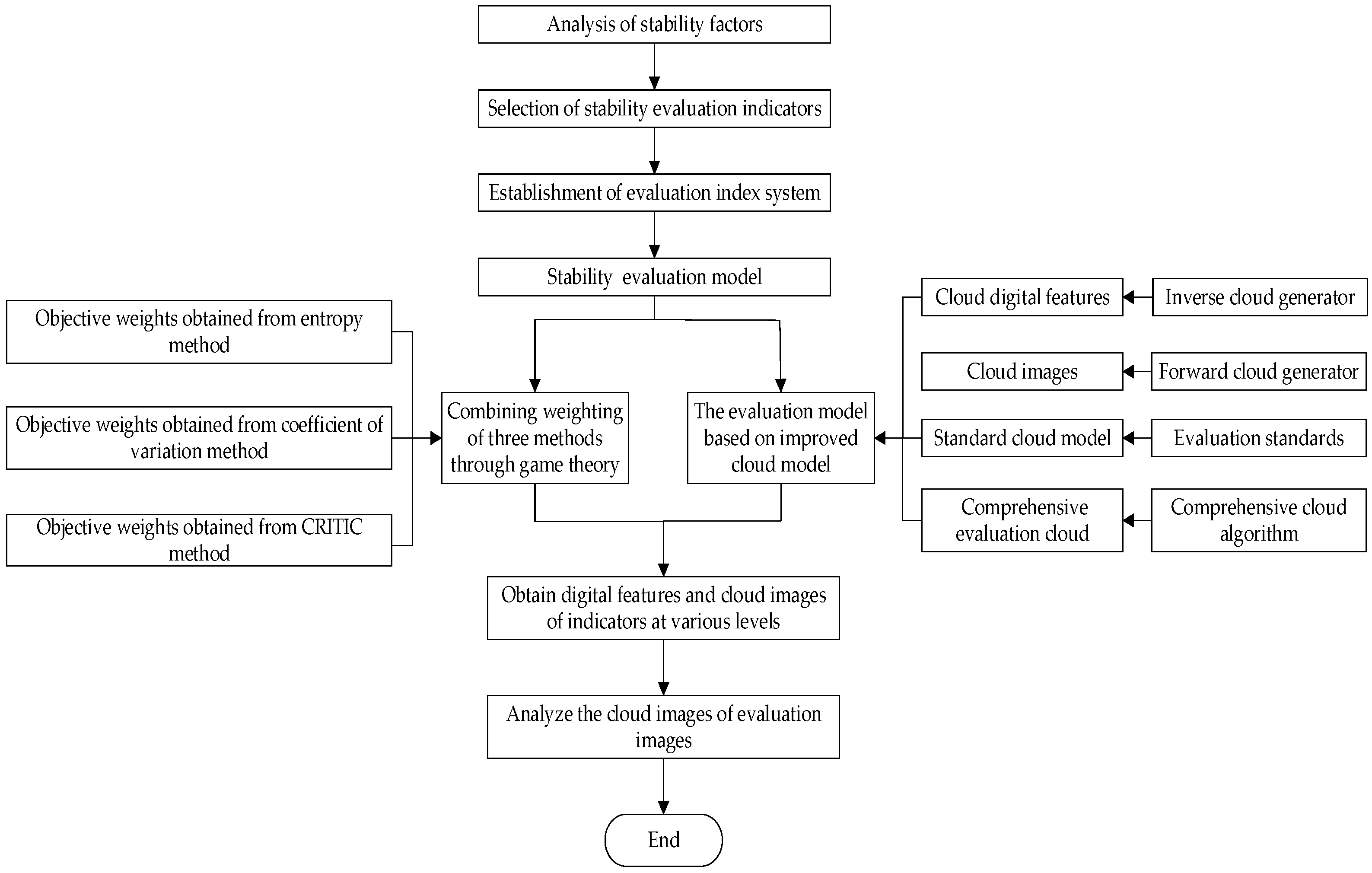
3. Evaluation Model for Stability

In order to better evaluate the stability of the new electric power system, assess its vulnerability, and give suggestions for improvement, a stability evaluation model of a new electric power system is constructed based on the combined weighting method of game theory and an improved cloud model. The specific process can be seen in Figure 1.

In the weighting process of multi-indicator evaluation systems, commonly used single weighting methods are often one-sided and limited. Therefore, three objective weighting methods are used for combined weighting in this research. The combination weighting in game theory can co-ordinate conflicts and contradictions between evaluation objectives, minimize the error of indicator weights, and obtain balanced combination weights. The final weight obtained by combination weighting in game theory is objective and reasonable.

To address the uncertainty of indicator objects, a cloud model is employed in this research. This model reveals the inherent correlation between the randomness and fuzziness of evaluation objectives. Moreover, it can visually displays the stability level of the electric power system through cloud images, achieving the conversion of qualitative and quantitative concepts.

Figure 1 depicts the flow of our model for evaluating stability. First, a system of indices for evaluating stability is constructed. Then, based on the actual data of the indicators, the respective weights are determined by including the entropy value method, the coefficient of variation method, and the CRITIC method. These weights are combined to form optimal portfolio weights using game theory. After that, the improved cloud model is used to evaluate stability, in which cloud digital features are produced by an inverse cloud generator and cloud images of evaluation metrics are generated by a forward cloud generator. Finally, the evaluation cloud images of indicators at various levels are studied and analyzed.

3.1. Index Weight Setting Based on Game Theory

Game theory, which focuses on the interactions between formulaic incentive structures, is a mathematical theory and methodology for studying phenomena of a combative or competitive nature [37]. In the specific field of combining weights for the evaluation of electric power systems’ stability, game theory is the best method of obtaining optimal portfolio weights.

In the process of empowering multi-indicator system assessment, a combination of subjective and objective empowerment methods is often used. However, each assignment method has its own advantages and limitations. In order to minimize the subjective error of the results, three objective assignment methods (the entropy weight method, coefficient of variation method, and CRITIC method) will be used for the combination of assignment. This method makes up for the subjectivity of the subjective assignment method and the insufficiency of one assignment method alone, which can effectively reduce the ambiguity and randomness in the comprehensive evaluation and make the evaluation results more real and reliable.

In the comprehensive evaluation research, the weights of indicators play a crucial role in the rationality and accuracy of the final evaluation results, and the combination assignment method reduces the loss of evaluation information as much as possible, making the results of combination weight calculation more objective and practical. Therefore, game theory is chosen for combination assignment to establish an objective link between indicators and improve the objectivity of weight assignment. In order to account for the conflicting nature of various objective assignment methods, the three selected weight calculation methods are used to complement each other, so that the optimal weight combination can be obtained by establishing a Nash equilibrium through game theory.

This section describes the theoretical foundations and methodology of portfolio empowerment based on game theory. The specific computational steps of the evaluation model based on the game-theory-improved cloud model can be found below.

3.1.1. Indicator Weight Calculation Method

In order to obtain more accurate indicator weights, three objective assignment methods, including entropy, CRITIC, and coefficient of variation, are used to calculate the indicator weights. The basic steps are as follows.

First step: In order to solve the evaluation result error caused by the difference in the unit of each index, the data are first normalized. For specific steps, refer to study [38].

Second step: The entropy weight method calculates the indicator weights according to the amount of information contained in the indicators. For specific steps, refer to study [39].

Third step: The CRITIC method expresses the amount of information through the contrast and degree of conflict between indicators to determine the weight of indicators. For specific steps, refer to study [40].

Fourth step: The coefficient of variation method can directly obtain the objective information weights of different evaluation indicators based on the degree of difference of the data. For specific steps, refer to study [41].

3.1.2. Combination Weighting Theory Method Based on Game Theory

The game theory is used to combine the weights calculated by various methods and optimize these weights to obtain an optimal combination of weights. On the one hand, this method can combine the advantages of various assignment methods. On the other hand, it can also overcome the limitations of each weight calculation method in order to obtain more accurate indicator weights. Game theory focuses on the interaction between formulaic incentive structures and is a mathematical theory and method for studying phenomena with the nature of conflict or competition. Since objective assignment methods have their own advantages and disadvantages, in order to resolve the conflicting nature of various methods and retain their consistency, a Nash equilibrium is established to obtain an optimal combination of weights by combining game theory. The specific process of reaching this equilibrium can be described as follows [27].

First step: Weight sets are constructed.

For multi-index decision-making problems, multiple methods are often used to determine index weights to ensure more accurate conclusions, for which a vector set is constructed: $W=\left\{w_1,w_2,w_3\right\}$. The combined weights W of the three weight vectors are

$$W={\beta }_1{w}_1+{\beta }_2{w}_2+{\beta }_3{w}_3,$$

(41)

where $w_1$, $w_2$, and $w_3$ represent the indicator weights of the entropy weight method, critic method and coefficient of variation method, respectively. ${\beta }_1$, ${\beta }_2$, and ${\beta }_3$ represent the linear combination coefficients of these three objective assignment methods.

Second step: The optimal weight vector is obtained.

The optimal weight vector is obtained by optimizing the linear combination of coefficients to minimize the deviation of ${\beta }_1$, ${\beta }_2,$ and ${\beta }_3$.

$${\mathrm{m}\mathrm{i}\mathrm{n}\left|\left|W-w\right|\right|}^2$$

(42)

Third step: The system of first-order linear equations is set up.

From the nature of matrix differentiation, the above equation is equated to a system of first-order linear equations with optimal derivative conditions.

$$\left[\begin{array}{ccc}{w}_1{w}_1^T& w_1{w}_2^T& w_1{w}_3^T\\ w_2{w}_1^T& w_2{w}_2^T& w_2{w}_3^T\\ w_3{w}_1^T& w_3{w}_2^T& w_3{w}_3^T\end{array}\right]\left[\begin{array}{c}{\beta }_1\\ {\beta }_2\\ {\beta }_3\end{array}\right]=\left[\begin{array}{c}{w}_1{w}_1^T\\ w_2{w}_2^T\\ w_3{w}_3^T\end{array}\right],$$

(43)

Fourth step: The portfolio weights are obtained.

$$W={\displaystyle \frac{{\beta }_1}{{\beta }_1+{\beta }_2+{\beta }_3}}{w}_1+{\displaystyle \frac{{\beta }_2}{{\beta }_1+{\beta }_2+{\beta }_3}}{w}_2+{\displaystyle \frac{{\beta }_3}{{\beta }_1+{\beta }_2+{\beta }_3}}{w}_3.$$

(44)

3.2. Stability Evaluation Model Based on an Improved Cloud Model

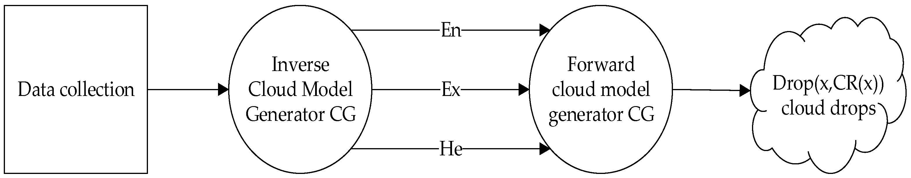
The research objectives involved in evaluating the stability of the new electric power system have ambiguity and randomness, so solving the uncertainty of the research object is a huge challenge. The cloud model may be able to realize the natural transformation from quantitative to qualitative analysis. In addition, the evaluation results of the cloud model are cloud images, which can more intuitively show the evaluation results. Moreover, the cloud model can be comprehensively analyzed and evaluated from multiple perspectives, which ensures the rationality of the comprehensive evaluation results.

3.2.1. Basic Theory

The cloud model was established by academician Li Deyi based on the theory of stochastic and fuzzy mathematics. This model well reflects the fuzzy and random nature of the evaluation objects [42]. The cloud image consists of three cloud digital features, including expectation Ex, entropy En, and superentropy He, which express the quantitative characteristics of qualitative concepts. Ex reflects the center of distribution of cloud droplets, which is able to portray the center of the transformation from quantitative to qualitative analysis. En indicates the range of dispersion of the cloud droplets, and He denotes the degree of stability of the cloud droplets, which embodies the uncertainty of entropy.

The cloud generator is the key to the practical application of cloud model theory, which can be divided into a forward cloud and inverse cloud generator according to the working mechanism. The forward cloud generator is used to realize the transformation from qualitative to quantitative concepts [43]. The inverse cloud generator is used to transform from quantitative to qualitative concepts [44]. The specific process is shown in Figure 2.

The inverse cloud generator is utilized to compute the evaluated cloud’s digital features, and the steps of the algorithm are as follows [44]:

First step: the mean value is calculated.

$$Ex=\overline{x}={\displaystyle \frac{1}{n}}{\sum }_{i=1}^n{x}_i,$$

(45)

where $x_i$ represents the ith data of the indicators, n represents the number of data contained in the indicators, and $\overline{x}$ represents the average value of the data for the indicators.

Second step: the variance S is calculated.

$$S=\sqrt{{\displaystyle \frac{1}{n-1}}{\sum }_{i=1}^n{\left(x_i-\overline{x}\right)}^2},$$

(46)

Third step: the cloud digital features are calculated.

$$\left\{\begin{array}{c}Ex=\overline{x}\\ En=\sqrt{{\displaystyle \frac{\pi }{2}}}{\displaystyle \frac{1}{n}}{\sum }_{i=1}^n\left|x_i-\overline{x}\right|\\ He=\sqrt{S^2-{En}^2}\end{array}\right..$$

(47)

The forward cloud generator is utilized to generate the cloud image, and the steps of the algorithm are as follows [43]:

First step: normal random numbers ${\mathrm{E}\mathrm{n}}^{\ast }$ and ${\mathrm{E}\mathrm{n}}^{\ast }~N\left(\mathrm{E}\mathrm{n},{\mathrm{H}\mathrm{e}}^2\right)$ are generated.

Second step: normal random numbers x and $x~N\left(\mathrm{E}\mathrm{x},{\mathrm{E}\mathrm{n}}^{\ast 2}\right)$ are generated.

Third step: the cloud droplets $\mathrm{e}\left(x,\mu \left(x\right)\right)$ and degree of affiliation $\mu \left(x\right)={\mathrm{e}}^{-{\displaystyle \frac{{\left(x-\mathrm{E}\mathrm{x}\right)}^2}{2{\left({\mathrm{E}\mathrm{x}}^{\ast }\right)}^2}}}$ are generated.

MATLAB 2023b software is used to implement the forward cloud model algorithm in order to present related images of evaluation grades through three cloud digital features.

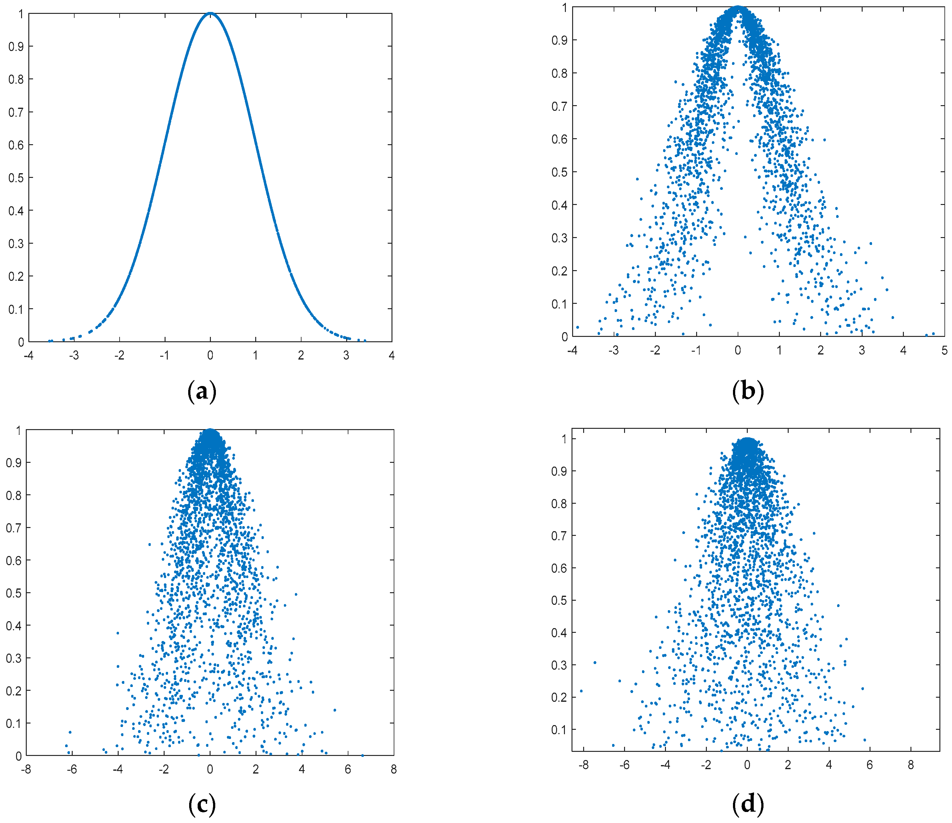
3.2.2. The 3En Criterion of the Cloud Model

The digital features U(Ex,En,He) of the cloud model determine the basic characteristics of the cloud model image. When He = 0, the cloud droplets of the cloud model image completely obey the Gaussian curve and are normally distributed [43,44]. As the He value gradually increases, the cohesion of the cloud droplets decreases, and the droplets gradually disperse. This process is called cloud atomization, and the specific process is shown in Figure 3.

The cloud model has the “3En” criterion, that is, the probability that a cloud drop falls in the interval [En − 3He,En + 3He] is 99.7%. When He < En/3, the cloud droplet obeys a normal distribution. When He > En/3, the cloud droplet distribution starts to atomize; when He = En/3, the cloud droplets present a critical value of atomization.

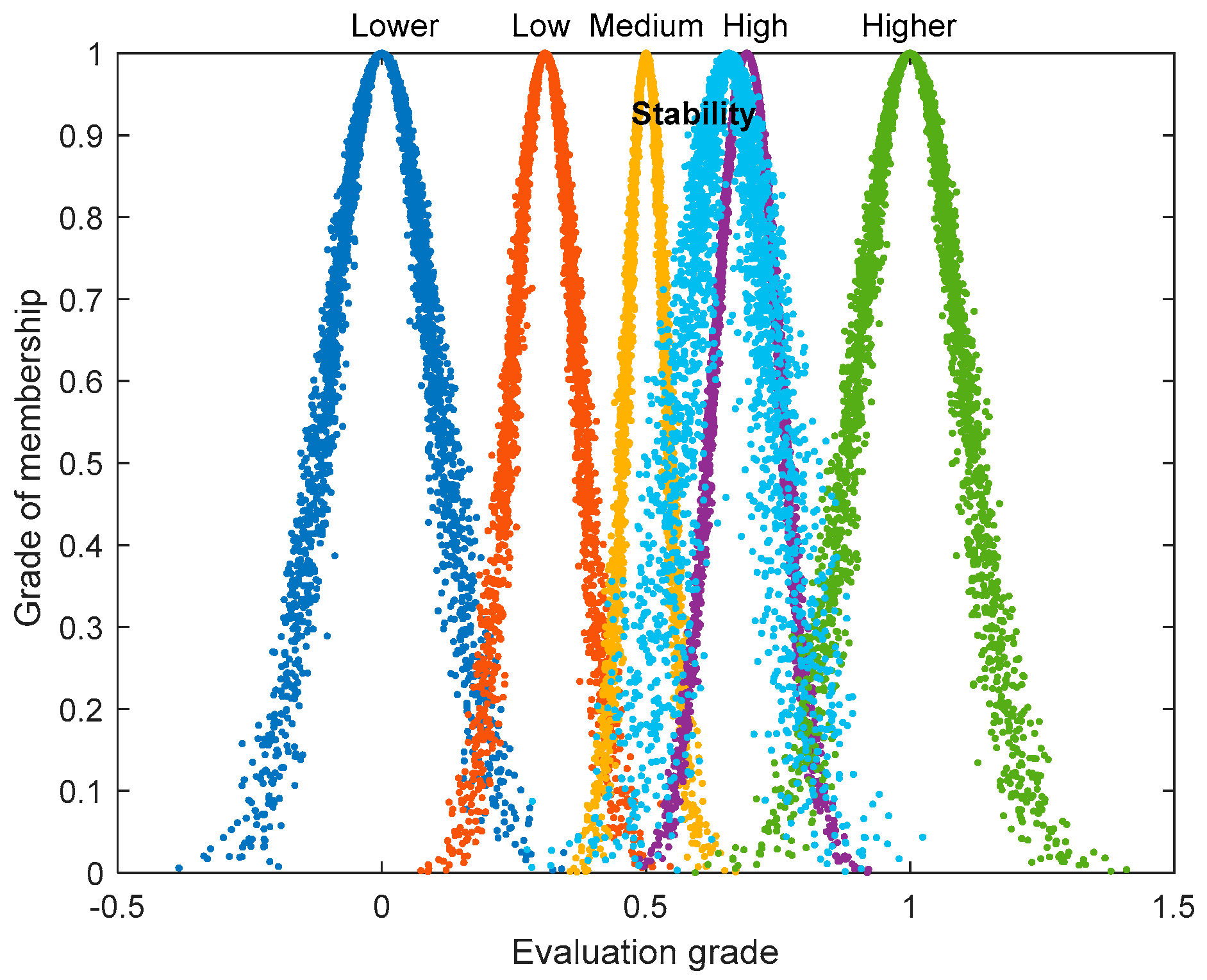
3.2.3. Determination of Standard Cloud Model

The evaluation criteria cloud is a baseline comparison chart for adaptation evaluation. The evaluation levels of adaptation are categorized as “lower”, “lower”, “medium”, “high”, and “higher”. The “golden section” method is used to classify the stability level interval of the new electric power system, and the ratio between the parameters of the cloud model of the neighboring evaluation levels is 0.618 [45]. The hyperentropy value He of the “medium” level is set to 0.003, and the symmetry is taken into account. The parameters of each evaluation level are listed in

Table 2. Standard cloud model for stability evaluation.

Evaluation Standard	Cloud Model Feature Parameters
Lower	(0.000, 0.103, 0.008)
Low	(0.309, 0.064, 0.005)
Medium	(0.500, 0.039, 0.003)
High	(0.691, 0.064, 0.005)
Higher	(1.000, 0.103, 0.008)

, and the standard cloud image is shown in Figure 4.

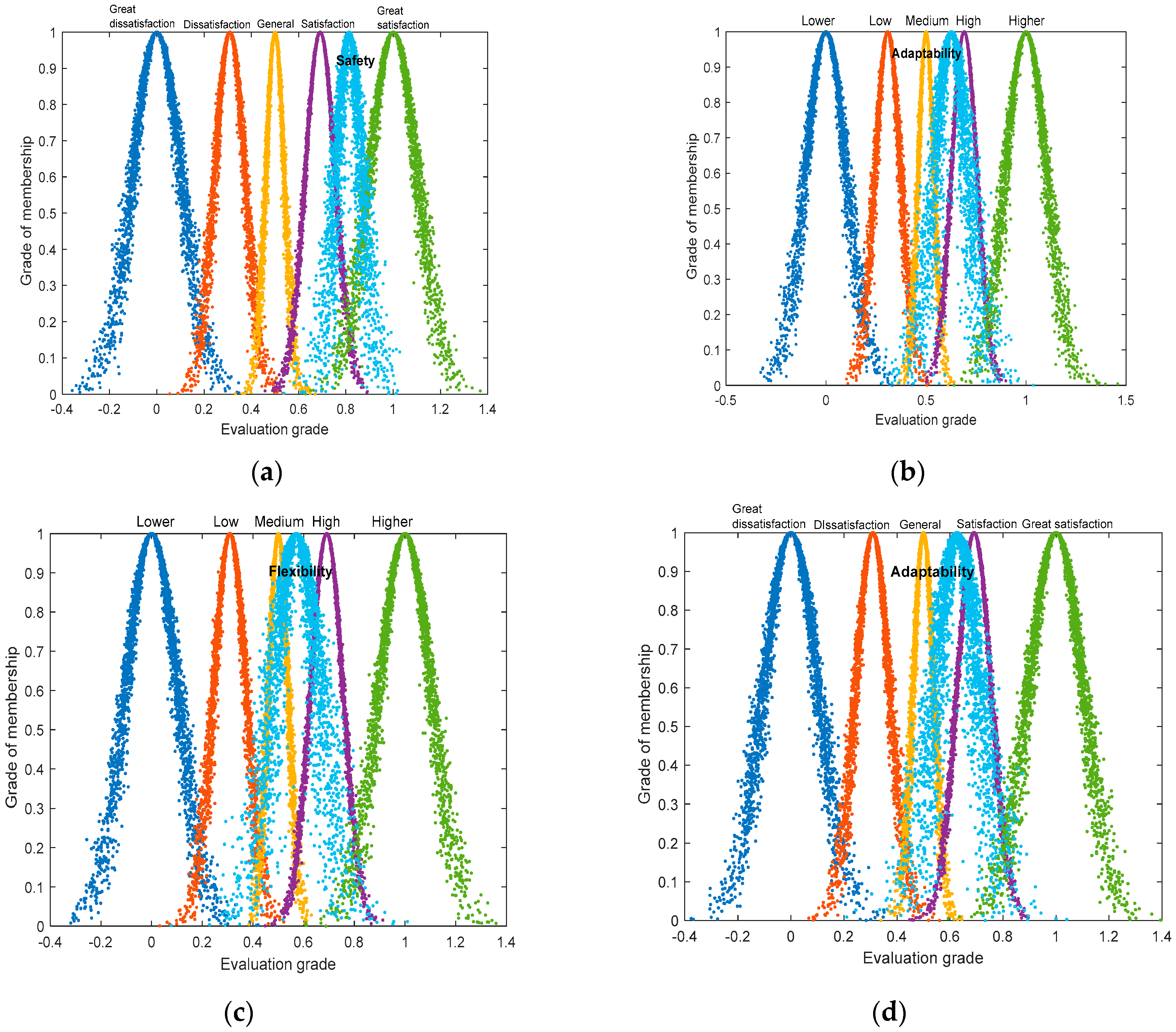
3.2.4. Comprehensive Cloud Evaluation

In order to accurately assess the stability of the new electric power system, a comprehensive cloud algorithm is required, which in turn leads to the cloud digital features of the first-level and second-level indicators [43,44].

When the degree of correlation between the indicators is low, the floating cloud algorithm is used to solve the problem, and the formula is as follows:

$$\left\{\begin{array}{c}\mathrm{E}\mathrm{x}={\displaystyle \frac{{\mathrm{E}\mathrm{x}}_1{w}_1+{\mathrm{E}\mathrm{x}}_2{w}_2+\cdots +{\mathrm{E}\mathrm{x}}_{\mathrm{m}}{w}_m}{w_1+w_2+\cdots +w_m}}\\ \mathrm{E}\mathrm{n}={\displaystyle \frac{{\mathrm{E}\mathrm{n}}_1{w}_1^2+{\mathrm{E}\mathrm{n}}_2{w}_2^2+\cdots +{\mathrm{E}\mathrm{n}}_{\mathrm{m}}{w}_m^2}{w_1^2+w_2^2+\cdots +w_m^2}}\\ \mathrm{H}\mathrm{e}={\displaystyle \frac{{\mathrm{H}\mathrm{e}}_1{w}_1^2+{\mathrm{H}\mathrm{e}}_2{w}_2^2+\dots +{\mathrm{H}\mathrm{e}}_{\mathrm{m}}{w}_m^2}{w_1^2+w_2^2+\dots +w_m^2}}\end{array}\right..$$

(48)

When the degree of correlation between the indicators is high, the integrated cloud algorithm is used, and the formula is as follows:

$$\left\{\begin{array}{l}\mathrm{E}\mathrm{x}={\displaystyle \frac{{\mathrm{E}\mathrm{x}}_1{\mathrm{E}\mathrm{n}}_1{w}_1+{\mathrm{E}\mathrm{x}}_2{\mathrm{E}\mathrm{n}}_2{w}_2+\cdots +{\mathrm{E}\mathrm{x}}_{\mathrm{m}}{\mathrm{E}\mathrm{n}}_{\mathrm{m}}{w}_m}{{\mathrm{E}\mathrm{n}}_1{w}_1+{\mathrm{E}\mathrm{n}}_2{w}_2+\cdots +{\mathrm{E}\mathrm{n}}_{\mathrm{m}}{w}_m}}\\ \mathrm{E}\mathrm{n}={\mathrm{E}\mathrm{n}}_1{w}_1+{\mathrm{E}\mathrm{n}}_2{w}_2+\cdots +{\mathrm{E}\mathrm{n}}_{\mathrm{m}}{w}_m\\ \mathrm{H}\mathrm{e}={\displaystyle \frac{{\mathrm{H}\mathrm{e}}_1{\mathrm{E}\mathrm{n}}_1{w}_1+{\mathrm{H}\mathrm{e}}_2{\mathrm{E}\mathrm{n}}_2{w}_2+\cdots +{\mathrm{H}\mathrm{e}}_{\mathrm{m}}{\mathrm{E}\mathrm{n}}_{\mathrm{m}}{w}_m}{{\mathrm{E}\mathrm{n}}_1{w}_1+{\mathrm{E}\mathrm{n}}_2{w}_2+\cdots +{\mathrm{E}\mathrm{n}}_{\mathrm{m}}{w}_m}}\end{array}\right..$$

(49)

where $w_m$ is the combined weights of the mth indicators; m is the total number of indicators evaluated.

4. Results

4.1. Basic Data and Scenario Setting

In order to accelerate the construction of the new electric power system, Zhejiang Provincial Development and Reform Commission have issued the “14th Five-Year Plan for renewable energy development in Zhejiang Province” alongside other notification documents [46,47]. Zhejiang Province has vigorously planned to develop wind power and photovoltaic power but also to engage more in pumped storage-based hydropower regulation at the same time, according to local conditions and high-quality development of biomass energy. By the end of 2025, the new energy installed capacity is predicted to reach more than 58.6%, and photovoltaic power is predicted to become the first new energy power source with an installed capacity of more than 28.6%, while new energy power generation is predicted to reach more than 50%.

Taking a county-level pilot program of integrating source, network, load, and storage in Zhejiang Province, China, as an example in this study, data for three years from 2020 to 2022 are selected for analysis. The following are some facts about this pilot program. The power supply area of this grid is 1067 square kilometers, and the power supply population is about 418,600 people. This area is a 110 kV power grid with a single ring structure, and it is part of the Fukushima area, featuring T-connections. There are 9110 kV transformer substations and 24 main transformers with a capacity of 1100 MVA. There are 270,110 kV lines with a total length of 2600 km, of which the overhead length is 1257.36 km and the cable length is 854 km.

Under different time periods and other conditions, the various parameters and calculation indices of the power grid will be very different. Therefore, a typical scenario is chosen to calculate the corresponding evaluation index, and a typical day of load measurement, that is, 13:00–14:00 (hereinafter referred to as the “typical day”), is selected for each year. Subsequently, the data of the typical day of these three years are processed and analyzed.

4.2. Index Weight Calculation

Firstly, three years of actual data from a county-level pilot program in Zhejiang, China, are normalized. Then, the entropy method, coefficient of variation method, and CRITIC method are used to calculate the weights of each index through the formulas in the corresponding literature. Finally, the combination weights of these three objective assignment methods are applied based on game theory. Equations (41)–(44) are utilized to obtain the weights of the third-level indicators. The weight results of each level are shown in

Table 3. Weights of evaluation indicators at each level.

First-Level Indicators	Weight	Second-Level Indicators	Weight	Third-Level Indicators	Entropy Method	Coefficient of Variation Method	CRITIC Method	Combined Weight
A	0.237	${\mathrm{A}}_1$	0.100	${\mathrm{a}}_{11}$	0.024	0.024	0.022	0.023
				${\mathrm{a}}_{12}$	0.060	0.046	0.025	0.049
				${\mathrm{a}}_{13}$	0.028	0.029	0.025	0.028
		${\mathrm{A}}_2$	0.088	${\mathrm{a}}_{21}$	0.025	0.025	0.044	0.027
				${\mathrm{a}}_{22}$	0.029	0.029	0.044	0.031
				${\mathrm{a}}_{23}$	0.032	0.032	0.021	0.030
		${\mathrm{A}}_3$	0.049	${\mathrm{a}}_{31}$	0.024	0.024	0.040	0.026
				${\mathrm{a}}_{32}$	0.023	0.023	0.021	0.023
B	0.163	${\mathrm{B}}_1$	0.080	${\mathrm{b}}_{11}$	0.024	0.025	0.019	0.024
				${\mathrm{b}}_{12}$	0.028	0.028	0.019	0.027
				${\mathrm{b}}_{13}$	0.030	0.030	0.020	0.029
		${\mathrm{B}}_2$	0.083	${\mathrm{b}}_{21}$	0.033	0.033	0.021	0.031
				${\mathrm{b}}_{22}$	0.030	0.030	0.020	0.029
				${\mathrm{b}}_{23}$	0.024	0.024	0.020	0.023
C	0.273	${\mathrm{C}}_1$	0.082	${\mathrm{c}}_{11}$	0.027	0.027	0.019	0.026
				${\mathrm{c}}_{12}$	0.025	0.026	0.044	0.028
				${\mathrm{c}}_{13}$	0.026	0.027	0.044	0.028
		${\mathrm{C}}_2$	0.080	${\mathrm{c}}_{21}$	0.026	0.027	0.019	0.026
				${\mathrm{c}}_{22}$	0.026	0.026	0.044	0.028
				${\mathrm{c}}_{23}$	0.027	0.027	0.019	0.026
		${\mathrm{C}}_3$	0.054	${\mathrm{c}}_{31}$	0.026	0.027	0.019	0.026
				${\mathrm{c}}_{32}$	0.025	0.026	0.044	0.028
		${\mathrm{C}}_4$	0.057	${\mathrm{c}}_{41}$	0.028	0.029	0.044	0.030
				${\mathrm{c}}_{42}$	0.025	0.025	0.044	0.027
D	0.327	${\mathrm{D}}_1$	0.114	${\mathrm{d}}_{11}$	0.021	0.023	0.016	0.021
				${\mathrm{d}}_{12}$	0.021	0.023	0.017	0.021
				${\mathrm{d}}_{13}$	0.022	0.025	0.016	0.024
				${\mathrm{d}}_{14}$	0.026	0.027	0.017	0.026
				${\mathrm{d}}_{15}$	0.023	0.022	0.016	0.022
		${\mathrm{D}}_2$	0.101	${\mathrm{d}}_{21}$	0.019	0.019	0.019	0.019
				${\mathrm{d}}_{22}$	0.020	0.020	0.018	0.019
				${\mathrm{d}}_{23}$	0.023	0.021	0.019	0.022
				${\mathrm{d}}_{24}$	0.020	0.024	0.016	0.021
				${\mathrm{d}}_{25}$	0.021	0.020	0.018	0.020
		${\mathrm{D}}_3$	0.110	${\mathrm{d}}_{31}$	0.022	0.020	0.031	0.022
				${\mathrm{d}}_{32}$	0.022	0.021	0.032	0.023
				${\mathrm{d}}_{33}$	0.021	0.020	0.022	0.021
				${\mathrm{d}}_{34}$	0.020	0.021	0.021	0.021
				${\mathrm{d}}_{35}$	0.026	0.025	0.022	0.023

.

4.3. Evaluation of the Improved Cloud Model

Improved cloud modeling is applied to assess the stability of the electric power system in a region in China. Based on the relevant national standards [48,49], the scoring curves of each indicator are derived, after which three years of data are preprocessed. The cloud digital characteristics of the third-level indicators are obtained by Equations (45)–(47). Then, combining the weights of the third-level indicators and the digital features of the third-level indicators, the digital features of the second-level indicator cloud are obtained by Equation (48). The same theory can be used to obtain the cloud digital features of the first-level indicators. The digital characteristics of each indicator are shown in

Table 4. Digital features of evaluation indicators at each level.

First-Level Indicators	Digital Features of Cloud Model (Ex,En,He)	Second-Level Indicators	Digital Features of Cloud Model (Ex,En,He)	Third-Level Indicators	Ex	En	He
A	(0.813, 0.055, 0.018)	${\mathrm{A}}_1$	(0.799, 0.052, 0.017)	${\mathrm{a}}_{11}$	0.947	0.057	0.018
				${\mathrm{a}}_{12}$	0.747	0.031	0.010
				${\mathrm{a}}_{13}$	0.767	0.114	0.037
		${\mathrm{A}}_2$	(0.844, 0.072, 0.023)	${\mathrm{a}}_{21}$	0.797	0.173	0.054
				${\mathrm{a}}_{22}$	0.943	0.006	0.002
				${\mathrm{a}}_{23}$	0.787	0.058	0.019
		${\mathrm{A}}_3$	(0.787, 0.031, 0.011)	${\mathrm{a}}_{31}$	0.827	0.020	0.007
				${\mathrm{a}}_{32}$	0.743	0.044	0.015
B	(0.702, 0.110, 0.031)	${\mathrm{B}}_1$	(0.679, 0.078, 0.021)	${\mathrm{b}}_{11}$	0.700	0.050	0.016
				${\mathrm{b}}_{12}$	0.667	0.086	0.024
				${\mathrm{b}}_{13}$	0.673	0.089	0.022
		${\mathrm{B}}_2$	(0.723, 0.157, 0.047)	${\mathrm{b}}_{21}$	0.707	0.086	0.028
				${\mathrm{b}}_{22}$	0.720	0.109	0.034
				${\mathrm{b}}_{23}$	0.750	0.359	0.099
C	(0.571, 0.091, 0.027)	${\mathrm{C}}_1$	(0.562, 0.122, 0.039)	${\mathrm{c}}_{11}$	0.637	0.170	0.056
				${\mathrm{c}}_{12}$	0.457	0.056	0.018
				${\mathrm{c}}_{13}$	0.597	0.145	0.044
		${\mathrm{C}}_2$	(0.507, 0.072, 0.023)	${\mathrm{c}}_{21}$	0.533	0.131	0.043
				${\mathrm{c}}_{22}$	0.477	0.047	0.014
				${\mathrm{c}}_{23}$	0.513	0.045	0.015
		${\mathrm{C}}_3$	(0.591, 0.103, 0.032)	${\mathrm{c}}_{31}$	0.617	0.178	0.055
				${\mathrm{c}}_{32}$	0.567	0.037	0.012
		${\mathrm{C}}_4$	(0.653, 0.063, 0.013)	${\mathrm{c}}_{41}$	0.590	0.084	0.014
				${\mathrm{c}}_{42}$	0.723	0.038	0.013
D	(0.627, 0.084, 0.026)	${\mathrm{D}}_1$	(0.647, 0.084, 0.025)	${\mathrm{d}}_{11}$	0.890	0.077	0.024
				${\mathrm{d}}_{12}$	0.603	0.047	0.014
				${\mathrm{d}}_{13}$	0.593	0.081	0.026
				${\mathrm{d}}_{14}$	0.640	0.075	0.021
				${\mathrm{d}}_{15}$	0.510	0.142	0.042
		${\mathrm{D}}_2$	(0.643, 0.115, 0.036)	${\mathrm{d}}_{21}$	0.627	0.114	0.033
				${\mathrm{d}}_{22}$	0.617	0.133	0.040
				${\mathrm{d}}_{23}$	0.747	0.153	0.051
				${\mathrm{d}}_{24}$	0.537	0.071	0.024
				${\mathrm{d}}_{25}$	0.683	0.103	0.032
		${\mathrm{D}}_3$	(0.570, 0.040, 0.013)	${\mathrm{d}}_{31}$	0.660	0.050	0.016
				${\mathrm{d}}_{32}$	0.523	0.035	0.012
				${\mathrm{d}}_{33}$	0.577	0.043	0.013
				${\mathrm{d}}_{34}$	0.575	0.042	0.012
				${\mathrm{d}}_{35}$	0.530	0.037	0.011

, and the corresponding cloud images are shown in Figure 5.

From the cloud images of the first-level indicators, the power system has the highest degree of safety with the highest affiliation of 0.813. It is followed by the evaluation results of adequacy and adaptability, both of which have a “high” evaluation level, with affiliation levels of 0.702 and 0.627, respectively. However, the evaluation cloud level for flexibility is closer to the “medium” level. It shows that the flexibility and adaptability of this power system need to be improved further. Due to the randomness of new energy generation and the tendency to generate harmonic distortion through power electronic components, the grid voltage will fluctuate or flicker. In order to minimize such problems, attention should be paid to the modification of electronic power equipment. In addition, due to the characteristics of energy storage technology, it is possible to deliver high-quality power to the grid or store excess power. In order to minimize the disadvantages associated with the high proportion of new energy sources connected to the grid, attention should also be paid to the improvement of energy storage equipment. Therefore, the model can identify the vulnerabilities of the new electric power system.

Combining the weights and digital characteristics of the first-level indicators, the numerical characteristics of the comprehensive evaluation are derived through Equation (49) as C(0.657, 0.085, 0.027). A cloud image of the comprehensive evaluation is obtained, as shown in Figure 6.

As can be seen from the above figure, the stability of this electric power system is closer to the “high” level, which is in line with the reality of the development of the region, and the evaluation results can intuitively reflect the evaluation results. Due to the potential improvement in the adaptability and flexibility of the electric power system, attention should be paid to the improvement and transformation of electronic power equipment and energy storage equipment, so as to reduce the disadvantages brought about by the high proportion of new energy connected to the grid. As a result, the evaluation model is able to identify the vulnerability of the electric power system more clearly, which provides advice for improving the stability of the new electric power system.

4.4. Comparison and Analysis

In order to verify the effectiveness of the improved cloud model, we compare the traditional cloud model with the improved cloud model. The weights of all indicators in the traditional cloud model are the same. The digital features of four first-level indicators are denoted $U_{\mathrm{A}}^{\ast }$, $U_{\mathrm{B}}^{\ast }$, $U_{\mathrm{C}}^{\ast }$, and $U_{\mathrm{D}}^{\ast }$ according to the traditional cloud model theory. The digital characteristics of comprehensive evaluation are denoted $U^{\ast }$. Then, the digital features of the first-level indicators are derived according to the traditional cloud model theory: $U_{\mathrm{A}}^{\ast }=\left(\mathrm{0.820,0.063,0.020}\right)$, $U_{\mathrm{B}}^{\ast }=\left(\mathrm{0.703,0.130,0.047}\right)$, $U_{\mathrm{C}}^{\ast }=\left(0.571,0.093,0.032\right)$, and $U_{\mathrm{D}}^{\ast }=\left(0.628,0.086,0.030\right)$. It is obvious that the digital characteristics of adequacy and flexibility do not satisfy the criterion of $\mathrm{H}\mathrm{e}<\mathrm{E}\mathrm{n}/3$. Finally, the digital characteristics of comprehensive evaluation are calculated as $U^{\ast }=\left(\mathrm{0.659,0.059,0.035}\right)$, and the corresponding cloud image is shown in Figure 7.

As can be seen from the above figure, the comprehensive evaluation result of the traditional cloud model is “high”, which is consistent with the evaluation result of the improved cloud model. However, it is clear that the evaluation result of the traditional cloud model appears to have atomization characteristics. The phenomenon of $\mathrm{H}\mathrm{e}>\mathrm{E}\mathrm{n}/3$ occurs, which leads to the poor performance of the cloud model’s atomization characteristics, and the evaluation results can not be used directly. Therefore, the improved cloud model has good validity, so that it can further improve the atomization characteristics of the traditional cloud model and enhance the credibility of the evaluation results without affecting the initial evaluation results, taking into account the differences between the indicators.

5. Discussion

From the above description, the following points can be summarized:

(1)

The feasibility and applicability of the model proposed in this paper are verified by the results of the arithmetic examples. Meanwhile, the evaluation results provide a basis for identifying the vulnerability of new electric power system.

(2)

The evaluation results show that the stability of the electric power system in the region can be improved. Measures such as the improvement and modification of electronic power equipment and energy storage equipment can be used to minimize the adverse effects of a high proportion of new energy sources connected to the grid, which will improve the stability of the new electric power system.

(3)

The applicability and superiority of the improved cloud model are highlighted by comparing the conventional cloud model with the improved cloud model and finding that the improved cloud model improves the atomization characteristics.

The evaluation results can validate the reliability of the model proposed in this paper and provide recommendations for improving the stability of new electric power systems and promoting sustainable development. However, the research in this paper also has shortcomings. In future research, it should be considered that the evaluation index system can be further optimized to ensure that all the indices can be applied by grid statisticians to actual electric power system statistics.

6. Conclusions

Based on analyzing the factors influencing the stability of the new electric power system, an evaluation method based on a game-theory-improved cloud model is proposed in this paper.

Firstly, new evaluation indices reflecting the characteristics of the new electric power system—such as new energy volatility, charge and discharge efficiency of energy storage, the reduction of new energy emissions, and so on—are innovatively proposed. The stability evaluation index system containing 4 first-level indices, 12 s-level indices and 39 third-level indices is constructed and complements the evaluation system.

Secondly, a combination of three objective assignment methods is assigned based on game theory to avoid subjectivity and bias in the evaluation results and reduce the ambiguity of information, which guarantees the reliability of the combined weighted results.

Finally, the improved cloud model can comprehensively visualize the stability of the power system through various levels of evaluation, integrated cloud images, and cloud digital features. The calculated values of the indices can reflect the vulnerability of the new electric power system and improve on specific recommendations for improving its stability.

In summary, it can be proven that the model can reflect the actual situation of the new electric power system through examples, which verifies the feasibility and accuracy of the model proposed in this paper. The model can provide suggestions for improving the stability of the new electric power system, which can promote energy transition and sustainable development.

References

1. Fan, R.Q.; Yang, Y.; Xu, K.; Xu, W.T. An overview of typical characteristics and development challenges of new power systems under the “dual-carbon” goal. Sichuan Electr. Power Technol. 2023, 46, 10–14+58. [Google Scholar]
2. Ren, D.W.; Xiao, J.Y.; Hou, J.M.; Du, E.S.; Jin, C.; Liu, Y. Construction and evolution of China’s new power system under dual carbon goal. Power Syst. Technol. 2022, 46, 3831–3839. [Google Scholar]
3. Hong, J.J.; Wang, Z.H.; Li, J.L.; Xu, Y.F.; Xin, H. Effect of Interface Structure and Behavior on the Fluid Flow Characteristics and Phase Interaction in the Petroleum Industry: State of the Art Review and Outlook. Energy Fuels 2023, 37, 9914–9937. [Google Scholar] [CrossRef]
4. Xu, Y.T.; Tan, Z.K.; Yuan, X.F.; Xie, B.M.; Chen, Y.F.; Wu, H. Power flow calculation for unbalanced distribution networks considering distributed generations. Electr. Meas. Instrum. 2019, 56, 27–32+80. [Google Scholar]
5. Liu, K.C.; Zhong, M.; Zeng, P.L.; Zhu, L.G. Review on reliability assessment of smart distribution networks considering distributed renewable energy and energy storage. Electr. Meas. Instrum. 2021, 58, 1–11. [Google Scholar]
6. Zheng, W.Y. Research on Static Voltage Stability Evaluation System of AC-DC Hybrid Power Grid. Bachelor’s Thesis, Shenyang Institute of Engineering, Shenyang, China, 2021. [Google Scholar]
7. Li, W.H.; Zhao, D.M.; Wang, X.; Yu, H. Adaptability evaluation for the distribution equipment considering distributed generations. Power Syst. Clean Energy 2017, 33, 117–123. [Google Scholar]
8. Huang, Q.H.; Wang, X.L.; Fan, J.J.; Wang, Y.F. Reliability and economy assessment of offshore wind farms. J. Eng. 2019, 16, 1554–1559. [Google Scholar] [CrossRef]
9. Research on the New Power System Index System. Available online: http://kns.cnki.net/kcms/detail/10.1289.TM.20231012.1633.014.html (accessed on 16 October 2023).
10. Yang, B.F. Construction and application of post evaluation system for provincial major power grid engineering investment projects. Money China 2022, 34, 72–74. [Google Scholar]
11. Zhang, M.; Xia, R.P.; Xu, S.L.; Lu, D.L.; Hu, Y.S. Comprehensive evaluation of power quality based on variation coefficient synthetic weighting of subjective and objective weights. Mod. Electr. Power 2023, 40, 441–447. [Google Scholar]
12. Zhu, Y.; Liu, X.; Mu, X.B.; Dai, F.J.; Xu, W.M.; Qian, W.J. Multi-index comprehensive evaluation of multi-station integrated energy system based on analytic hierarchy process and risk entropy weight. Electr. Meas. Instrum. 2022, 59, 128–136+143. [Google Scholar]
13. Ai, X.; Zhao, X.Z.; Hu, H.Y.; Wang, Z.D.; Peng, D.; Zhao, L. G1-entropy-independence weight method in situational awareness of power grid development. Power Syst. Technol. 2020, 44, 3481–3490. [Google Scholar]
14. Xiao, J.; Li, H.; Wang, B.; Song, C.H. Comprehensive matching evaluation method for integration of distributed generator into urban distribution network. Autom. Electr. Power Syst. 2020, 44, 44–51. [Google Scholar]
15. Lin, L.; Wang, T.Z.; Lv, Y.B.; Qu, S.J.; Gao, Z.H. Comprehensive evaluation of dispatching operation management level of distribution Network based on combined weight and gray cloud clustering model. J. North China Electr. Power Univ. (Nat. Sci. Ed.) 2022, 49, 31–40+80. [Google Scholar]
16. Pathan, M.I.; Alowaifeer, M.; Almuhaini, M.; Djokic, S.Z. Reliability evaluation of smart distribution grids with renewable energy sources and demand side management. Arab. J. Sci. Eng. 2020, 45, 6347–6360. [Google Scholar] [CrossRef]
17. Adaptability Evaluation of Distributed Photovoltaic Access Distribution Network. Available online: http://kns.cnki.net/kcms/detail/23.1202.TH.20220602.1656.006.html (accessed on 6 June 2022).
18. Liu, R.K.; Yao, J.; Pei, J.X.; Wang, X.W.; Sun, P.; Guo, X.L. Dynamic stability analysis of the weak grid connected DFIG based wind turbines under severe symmetrical faults. In Proceedings of the 2018 International Conference on Power System Technology (POWERCON), Guangzhou, China, 1 November 2018. [Google Scholar]
19. Power System Transient Stability Assessment Based on Probability Prediction and Intelligent Enhancement of MLE. Available online: http://kns.cnki.net/kcms/detail/11.2107.TM.20231007.1321.002.html (accessed on 8 October 2023).
20. Meridji, T.; Joos, G.; Restrepo, J. A power system stability assessment framework using machine learning. Electr. Power Syst. Res. 2023, 216, 108981. [Google Scholar] [CrossRef]
21. Cai, W.B.; Cheng, X.L.; Nan, J.N.; Lv, H.X.; Li, Y.; Li, J.Y. Assessment and analysis of adequacy of flexibility resource of power system with high proportion new energy. Electr. Drive 2022, 52, 57–62. [Google Scholar]
22. Zhang, L.Z.; Xu, T.; Song, S.Q.; Zhang, F. Evaluation method and guarantee mechanism of power generation capacity adequacy in electricity market. Autom. Electr. Power Syst. 2020, 44, 55–63. [Google Scholar]
23. Holttinen, H.; Tuohy, A.; Milligan, M.; Lannoye, E. The flexibility workout: Managing variable resources and assessing the need for power system modification. IEEE Power Energy Mag. 2013, 11, 53–62. [Google Scholar] [CrossRef]
24. Yang, L.J.; Li, H.Q.; Yu, X.Y.; Zhao, J.S.; Liu, W.Y. Multi-objective day-ahead optimal scheduling of isolated microgrid considering flexibility. Power Syst. Technol. 2018, 42, 1432–1440. [Google Scholar]
25. Chen, W.; Liu, Y.; Liu, X.Y. Transmission expansion planning considering adaptability of grid to short-circuit current. Sichuan Electr. Power Technol. 2018, 41, 74–77. [Google Scholar]
26. Du, M.K.; Huang, Y.; Liu, J.Y.; Lu, L.; Jiang, L.; Zhang, Q.M. Comprehensive evaluation on grid adaptability considering the access of cascaded power stations under planning and development. Proc. CSU-EPSA 2021, 33, 1–8+16. [Google Scholar]
27. Jia, W.J.; Luo, P. Power Supply and Distribution System; Chongqing University Press: Chongqing, China, 2016; pp. 260–265. [Google Scholar]
28. Yang, J.H.; Wu, J.H.; Saniye, M.; Zhang, H.; Yang, J. Research on security evaluation of power system with new energy. Mod. Electr. Power 2023, 40, 651–659. [Google Scholar]
29. Xu, J. Research on the capacity credibility of wind farms based on the reliability index LOLP. Energy Eng. 2011, 5, 38–40+49. [Google Scholar]
30. Research on Construction of Index System and Comprehensive Evaluation Method of Development Level of New Power System. Available online: https://www.chndoi.org/Resolution/Handler?doi=10.13335/j.1000-3673.pst.2023.2291 (accessed on 14 March 2024).
31. Xiao, Y.Y. Practical Research and Application of Large Power Grid Adequacy Assessment. Bachelor’s Thesis, Huazhong University of Science and Technology, Wuhan, China, 2018. [Google Scholar]
32. Li, J.H.; Long, Y.F.; Wen, J.Y.; Luo, W.H. Assessment of wind power capacity in power systems to meet the adequacy indexes. Power Syst. Technol. 2014, 38, 3396–3404. [Google Scholar]
33. Wang, H.K.; Wang, S.S.; Pan, Z.X.; Wang, J.M. Optimal scheduling method for flexibility enhancement of distribution networks containing high penetration distributed power source. Autom. Electr. Power Syst. 2018, 42, 86–93. [Google Scholar]
34. Wu, J.; Lu, Z.X.; Qiao, Y.; Yang, H.J. Optimisation of wind storage plant operation considering dynamic charging and discharging efficiency characteristics of energy storage plants. Autom. Electr. Power Syst. 2018, 42, 41–47+101. [Google Scholar]
35. National Energy Administration. Power Transformer Operation Regulations; China Electric Power Press: Beijing, China, 2010; pp. 15–19.
36. Li, S.X.; Zhou, B.X.; Tang, H.; Peng, Z.G. The improved algorithm model of capacity-load ratio in distribution network of remote areas. Electr. Meas. Instrum. 2016, 53, 27–31. [Google Scholar]
37. Li, T.H.; Xue, J.; Xia, W.; Ding, Y. Application of combination weighting method and comprehensive index method based on crack theory in ecological waterway assessment of Yangtze River ecological. J. Appl. Basic Eng. Sci. 2019, 27, 36–49. [Google Scholar]
38. Jiang, H.; Wu, J.H.; Saniye, M.; Zhang, Q.; Yao, L.; Kao, Y. Comprehensive vulnerability evaluation of power systems structure based on VIKOR method and complex network theory. Water Resour. Power 2023, 41, 216–220. [Google Scholar]
39. Liu, X.P.; Liu, M.H.; Huang, R.; Chen, X.Q.; Xu, H.T.; Xu, R.H. Research on performance evaluation method of smart energy meter based on grey correlation degree. Electr. Meas. Instrum. 2020, 57, 136–141. [Google Scholar]
40. He, T.; Ma, J. Reliability evaluation of CBTC based on cloud modeling and combination weighting method. J. Chongqing Univ. 2023, 46, 130–139. [Google Scholar]
41. Lin, G.Q.; Mo, T.W.; Ye, X.J.; Han, C.; Lin, Z.Z.; Wang, Z.K. Critical node identification of power networks based on TOPSIS and CRITIC methods. High Volt. Eng. 2018, 44, 3383–3389. [Google Scholar]
42. Li, D.Y.; Liu, C.Y. Study on the Universality of the Normal Cloud Model. Strateg. Study CAE 2004, 6, 28–34. [Google Scholar]
43. Yan, J.; Li, N.; Liu, Y.Q.; Li, L.; Kong, D.; Long, Q. Short-term uncertainty forecasting method for wind power based on real-time switching cloud model. Autom. Electr. Power Syst. 2019, 43, 17–23. [Google Scholar]
44. Yang, M.; Zhang, L.B.; Cui, Y.; Yang, Q.Q.; Huang, B.Y. Wind speed-power curve modeling method based on hybrid half-cloud model. Electr. Power Autom. Equip. 2020, 40, 106–112. [Google Scholar]
45. Cheng, J.T.; Duan, Z.M. Cloud model based sine cosine algorithm for solving optimization problems. Evol. Intell. 2019, 12, 503–514. [Google Scholar] [CrossRef]
46. On the Issuance of “Zhejiang Province Renewable Energy Development Fourteen Five-Year Plan” Notice. Available online: https://fzggw.zj.gov.cn/art/2021/6/23/art_1229123366_2305635.html (accessed on 23 June 2021).
47. On the Issuance of “Zhejiang Province, Renewable Energy Development “14th Five-Year Plan” Notice. Available online: https://fzggw.zj.gov.cn/art/2021/6/24/art_1229539890_4670809.html (accessed on 25 May 2021).
48. State Grid Corporation of China. The Guide of Planning and Design of Distribution Network; China Electric Power Press: Beijing, China, 2021; pp. 1–30. [Google Scholar]
49. China Southern Power Grid Company. Table of New Power System Technical Standard System and Roadmap for Standard Preparation Actions; China Electric Power Press: Beijing, China, 2022; pp. 10–50. [Google Scholar]
Figure 1. Model for evaluating stability.
Sustainability 16 06189 g001
Figure 2. Flow chart of cloud model.
Sustainability 16 06189 g002
Figure 3. The process of cloud atomization. Digital characteristics of the cloud models: (a) C(0,1,0); (b) C(0,1,0.33); (c) C(0,1,0.6); (d) C(0,1,1).
Sustainability 16 06189 g003
Figure 4. Standard cloud model image.
Sustainability 16 06189 g004
Figure 5. Evaluation cloud images for first-level indicators: (a) safety; (b) adequacy; (c) flexibility; (d) adaptability.
Sustainability 16 06189 g005
Figure 6. Cloud image of comprehensive evaluation.
Sustainability 16 06189 g006
Figure 7. Cloud image of comprehensive evaluation from the traditional cloud model.
Sustainability 16 06189 g007