Article

Spatio-Temporal Evolution of Ecological Environment Quality Based on High-Quality Time-Series Data Reconstruction: A Case Study in the Sanjiangyuan Nature Reserve of China

by
Xingzhu Xiao
,
Yanxi Chen
,
Yongle Zhang
,
Min Huang
and
Hao Li
*
College of Resources, Sichuan Agricultural University, Chengdu 611130, China
*
Author to whom correspondence should be addressed.
Sustainability 2024, 16(14), 6231; https://doi.org/10.3390/su16146231 (registering DOI)
Submission received: 30 May 2024 / Revised: 15 July 2024 / Accepted: 17 July 2024 / Published: 21 July 2024
(This article belongs to the Section Environmental Sustainability and Applications)

Abstract

:
The Sanjiangyuan Nature Reserve of China (SNRC) is recognized as one of the most fragile and sensitive terrestrial ecosystems in China, posing challenges for obtaining reliable and complete Moderate Resolution Imaging Spectro Radiometer (MODIS) data for ecological environment quality (EEQ) monitoring due to adverse factors like clouds and snow. In this study, a complete high-quality framework for MODIS time-series data reconstruction was constructed utilizing the Google Earth Engine (GEE) cloud platform. The reconstructed images were used to compute the Remote Sensing based Ecological Index (RSEI) on a monthly scale in the SNRC from 2001 to 2020. The results were as follows: The EEQ of the study area exhibited a “first fluctuating decline, then significant improvement” trend, with the RSEI values increasing at a rate of 0.84%/a. The spatial pattern of the EEQ displayed significant spatial heterogeneity, characterized by a “low in the west and high in the east” distribution. The spatial distribution pattern of the RSEI exhibited significant clustering characteristics. From 2001 to 2020, the proportion of “high–high” clustering areas exceeded 35%, and the proportion of “low–low” clustering areas exceeded 30%. Poor ecological conditions are mainly associated with population agglomerations, cultivated land, unutilized land, and bare ground, while grasslands and forests have higher RSEI values. The result of the trend analysis revealed a significant trend in RSEI change, with 62.96% of the area significantly improved and 6.31% significantly degraded. The Hurst Index (HI) results indicated that the future trend of the RSEI is predominantly anti-persistence. The proportion of areas where the EEQ is expected to continue improving in the future is 33.74%, whereas 21.21% of the area is forecasted to transition from improvement to degradation. The results showed that the high-quality framework for MODIS time-series data reconstruction enables the effective continuous monitoring of EEQ over long periods and large areas, providing robust scientific support for long time-series data reconstruction research.

1. Introduction

The Sanjiangyuan Nature Reserve of China (SNRC) is the source of the Yangtze River, Yellow River, and Lancang River, widely known as the “Water Tower of China” [1]. This area holds a crucial and distinctive ecological position, featuring one of the world’s highest concentrations of large rivers, glaciers, snow mountains, permafrost, and plateau biodiversity [2]. Simultaneously, it stands as one of the most fragile and sensitive regions of China’s terrestrial ecosystems [3], occupying a special position in China’s ecological civilization construction. In the past few decades, under the influences of global climate warming and unreasonable human development and utilization activities, the ecosystem degradation of the SNRC has become increasingly apparent. This degradation is characterized by the year-to-year shrinkage of glaciers, vegetation deterioration, land desertification, soil erosion [4,5], and other escalating ecological and environmental issues, leading to a continuous deterioration of the ecological environment. In order to reinforce the ecological protection and construction of the SNRC and accelerate the construction of China’s national ecological security barrier, the SNRC was officially established in 2000, and the State Council in China officially approved the establishment of the Sanjiangyuan National Nature Reserve (SNNR) in 2003 [6]. In 2005, the ecological protection and construction project for the SNNR was initiated, implementing 22 ecological construction projects [7]. In the past two decades, how has the ecological environment quality (EEQ) of the SNRC changed under the combined effects of climate fluctuations and human activities? Additionally, what impact did the ecological protection and construction project for the SNNR have on the EEQ? These questions are of utmost importance and require thorough clarification. The existing research on the SNRC has predominantly focused on vegetation changes [6,8] and climate changes [9,10], with limited studies addressing the dynamic monitoring and analysis of its EEQ. Therefore, investigating the EEQ and its change trend in the SNRC is of great practical significance for formulating corresponding ecological protection policies and evaluating the effectiveness of ecological engineering projects.
Ecological environment quality (EEQ) assessment is a crucial method for quantitatively evaluating the strengths and weaknesses of the regional ecological environment and its impact, providing a fundamental basis for formulating sustainable socio-economic development planning and ecological environment protection strategies [11]. Remote sensing technology provides comprehensive, extensive, and continuous surface information at different scales, making it suitable for EEQ assessment [12]. Xu et al. [13] integrated four remote sensing ecological factors including greenness, heat, dryness, and wetness to construct the Remote Sensing based Ecological Index (RSEI) for the rapid, objective, and accurate monitoring of regional EEQ changes. This index has been widely applied in various fields [14,15,16,17,18]. Previous studies have predominantly utilized Landsat and Moderate Resolution Imaging Spectroradiometer (MODIS) remote sensing data as data sources to construct the RSEI [19,20]. The MODIS, an Earth-viewing sensor, continuously collects data in 36 spectral channels, ensuring nearly complete global coverage every two days. Additionally, the Landsat Program offers the longest continuous space-based record of Earth’s land, and the time-series data collected by the Landsat satellite can be leveraged to monitor and comprehend the dynamics of the Earth’s surface at a spatial scale. Although the RSEI constructed based on Landsat data boasts high spatial resolution, it is difficult to obtain continuous high-quality images within the 16-day revisit period of Landsat data, resulting in problems such as missing data, chromatic aberration, and time inconsistency [21]. This approach is more suitable for single-time calculations, but not ideal for large-scale [22] or long time-series EEQ assessments. In contrast, MODIS imagery offers a shorter revisiting period and broader coverage [23], accumulating a wealth of freely available long-term historical data [24]. It can effectively capture the spatial patterns of the large-scale RSEI and is well-suited for comprehensive large-area and long time-series EEQ research.
The MODIS data provides convenient conditions for conducting large-scale EEQ dynamic monitoring and assessment [18], but its data quality is affected by multiple factors in the process of acquisition. The spatio-temporal continuity of MODIS data is often affected by non-biological factors, such as unfavorable atmospheric conditions like clouds, the ozone, and atmospheric aerosols, as well as differences in sensor performance and revisit periods [25]. These factors can lead to the unreliable quality of certain pixels and the presence of outliers, which may produce signal noise, poor quality, missing data, and other associated issues. The direct utilization of such data could adversely affect the inversion of the RSEI and the performance of ecological monitoring. Therefore, it is imperative to address the time-series data by executing a series of processes, such as filling missing values, filtering, and smoothing, to reconstruct high-quality time-series data before employing MODIS data for RSEI research [21,26]. The existing research on interpolation primarily revolves around the estimation of invalid pixel values using valid pixel values [27]. Nonetheless, in scenarios where a substantial number of invalid pixel values are present, the sampling points become excessively “sparse”, leading to “pseudo-variation” [28]. Consequently, the accuracy of the RSEI calculation remains subject to significant limitations.
To address the issues of poor quality, outliers, and missing values in MODIS data, a complete high-quality framework for MODIS time-series data reconstruction utilizing the Google Earth Engine (GEE) cloud platform was constructed. The framework uses methods such as harmonic regression, Hampel filter, Singular Spectrum Analysis (SSA), and Whittaker Smoothing (WS) to obtain complete and high-quality month-to-month MODIS data. Using the reconstructed data, a time series of the RSEI was constructed to analyze the EEQ change trends and future sustainability of the SNRC over a period of 20 years. The objective is to reveal the spatio-temporal characteristics of EEQ in the study area and to provide a reference and scientific basis for evaluating the effectiveness of ecological protection and construction projects within the SNRC, which holds significant importance for the formulation of eco-environmental protection policies and the sustainable development of the SNRC.

2. Material and Methods
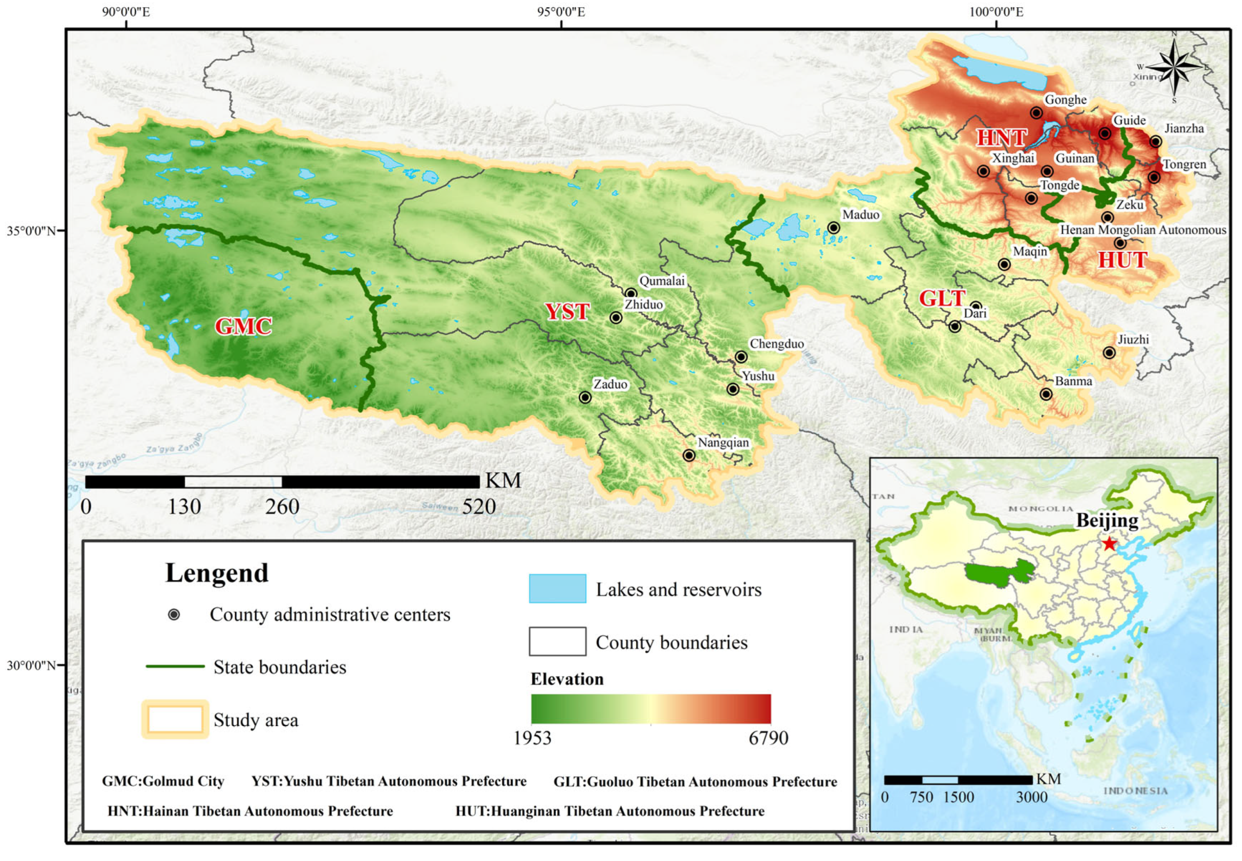
2.1. Study Area

The SNRC is situated in the heartland of the Qinghai–Tibet Plateau, in the southern part of Qinghai Province (Figure 1). It stands as the largest natural protected area in China, spanning between longitudes 89°24′ E and 102°23′ E and latitudes 31°39′ N and 36°16′ N, covering a total area of 366,000 square kilometers. The study area encompasses Golmud City (GMC), Yushu Tibetan Autonomous Prefecture (YST), Guoluo Tibetan Autonomous Prefecture (GLT), Hainan Tibetan Autonomous Prefecture (HNT), and Huangnan Tibetan Autonomous Prefecture (HUT), accounting for 43.88% of the total land area of Qinghai Province. The SNRC encompasses a multitude of lakes, boasting over 1800 in total, with 188 of these being natural lakes covering an area of more than 0.5 km2 [6]. The structure of the reserve is complex, since the economic activities of Tibetans, some of whom lead a nomadic lifestyle, are preserved on its territory. The climate falls under the Qinghai–Tibet Plateau system, with an annual average temperature varying from −5.6 to −7.8 °C and annual precipitation ranging from 262.2 to 772.8 mm. The topography of the region is predominantly plateaus and mountains, with an average elevation ranging from 3500 to 4800 m [2]. The predominant vegetation types comprise alpine grassland and alpine meadows, although coniferous forests and broad-leaved forests are also present. The natural conditions are harsh, and the ecological environment is fragile, which is difficult to recover from once it has been damaged [29]. It is also the habitat of many endangered animals and plants, and has important ecological significance [30]. Therefore, this study focuses on the SNRC as the primary area of investigation, representing a significant and essential locale for exploring the EEQ and its evolution trend within this region.

2.2. Data Sources

2.2.1. Remote Sensing Data

The MODIS, provided by the National Aeronautics and Space Administration (NASA), is one of the important sensors carried by the Terra and Aqua satellites [31]. It has the characteristics of high temporal resolution, spatial resolution, extensive historical data accumulation, and wide coverage [32], making it well-suited for monitoring past and present ecological conditions. Therefore, the study selected MODIS data to monitor the changes in EEQ and its evolution trend in the SNRC over the past two decades. Based on the Google Earth Engine (GEE) cloud platform, this study selected the MODIS Version 6.1 data products, including the surface reflectance product (MOD09A1), land surface temperature/emissivity (LST) products (MOD11A2), and vegetation index product (MOD13A1), all of which are carried aboard the Terra satellite (Table 1).

2.2.2. Fundamental Geographic Information

The 1:1 million public version of basic geographic information was obtained from the National Catalogue Service for Geographic Information of China. The vector boundary data of the SNRC [33] were sourced from the National Ecological Science Data Center. The digital elevation model (DEM) data were sourced from the Shuttle Radar Topography Mission (SRTM) digital elevation datasets provided by the Geospatial Data Cloud. Furthermore, the vector data of permanent water bodies were obtained from the 1:1 million public version of basic geographic information (Layer “BOUA” and “HYDA”), which was used for water mask processing to remove water bodies (Table 1).

2.3. Methods

2.3.1. High-Quality MODIS Time-Series Data Reconstruction Framework

The usability of MODIS remote sensing imagery is subject to several influencing factors, including cloud layers, shadows, and atmospheric conditions. While the MODIS data obtained from the GEE cloud platform has undergone initial atmospheric correction and other preprocessing steps, which have contributed to the improvement of data quality to some extent [34], it is unable to completely eliminate the effects of these influencing factors. As a result, the obtained time-series data may still display discontinuities or irregularities, often manifesting as irregular jagged patterns. Furthermore, the construction of time-series data inherently incorporates noise, missing values, and outliers [35], which can compromise the authenticity and completeness of MODIS data. Coupled with the presence of substantial snow, cloud cover, and glaciers in the SNRC, the data quality is affected to a greater extent in the cloud and snow cover areas, which detrimentally affects the stability of the RSEI time series and the efficacy of the ecological quality monitoring. Consequently, the reconstruction of MODIS time-series data assumes paramount importance. In order to mitigate the influence of poor data quality, outliers, and missing values on RSEI computations, a complete and high-quality framework for MODIS time-series data reconstruction was proposed in this study; the technology roadmap is shown in Figure 2. This framework encompasses data preprocessing, noise reduction, smoothing, and interpolation, with the objective of overcoming the interference of extreme ecological zones and cloud-covered areas on RSEI computations in large-scale regions.

Data Processing

The methodology for processing MODIS data on the GEE cloud platform and the necessary indicators for the computation of the RSEI are detailed in Table 2. MODIS remote sensing images within the SNRC from 2001 to 2020 were downloaded from the MODIS dataset hosted on the GEE cloud platform. Given that the dataset in the GEE cloud platform has undergone radiometric calibration, atmospheric correction, and geometric correction, the preprocessing procedure primarily involves date screening, resampling, projection transformation, image cropping, and image stitching subsequent to data acquisition. Meanwhile, owing to the substantial presence of lakes and rivers in the SNRC, a vector dataset derived from the 1:1 million basic geographic information of China was utilized to mask water bodies in order to mitigate the influence of surface water bodies on the wetness index, dryness index, and principal component loadings.
Subsequently, the quality assessment (QA) bands were employed to eliminate pixels with poor quality. The QA bands provided by each product record the quality information of each pixel data as bit flags, allowing the identification and masking of pixels with poor quality due to factors such as cumulus clouds, cloud shadows, and snow/ice cover. An analysis of missing time-series data revealed that the percentage of missing pixels for MOD09A1, MOD11A2, and MOD1A13 stands at 37.20%, 13.11%, and 32.33%, respectively. The number of high-quality observations of MOD09A1 and MOD13A1 in the study area is relatively low, with a lower stability compared to MOD11A2 due to cloud and snow cover. Figure 3 illustrates that each pixel of MOD09A1 and MOD11A2 contains 920 time point data over 20 years, with missing pixels in the time series reaching up to 255 time points, equating to a missing proportion of 27.72%; each pixel of MOD13A1 encompasses 460 time point data over 20 years, with missing pixels in the time series reaching up to 255 time points, resulting in a missing proportion of 55.43%.

Abnormal Pixel Detection

The identification of common issues in MODIS data is primarily based on QA band processing, such as clouds, shadows, and snow, but it is unable to eliminate all abnormal pixels completely. Therefore, this study, conducted on the GEE cloud platform, employs harmonic regression and the Hampel filter to detrend and detect outliers in the time series of four indicators. These approaches effectively remove outliers caused by data corruption, errors, or anomalies in real data, and also eliminate noise in the time series. These processes lay the foundation for reconstructing high-quality MODIS time-series data.
Detrending eliminates the influence of offsets generated by sensors during data acquisition, focusing the analysis on the inherent fluctuations of the data trend, effectively eliminating spurious correlations arising from long-term trends [40]. Even after the QA band processing, time-series data are still affected by various random interferences, potentially leading to abnormal pixels. Detrending mitigates the impact of these interferences, eradicating long-term trends and seasonal variations, thereby enhancing the accuracy of detecting abnormal pixels in subsequent analysis. Previous studies commonly employed linear regression for detrending. However, observations by Lu [41], Ols [42], and others have highlighted that traditional linear regression overlooks the influence of internal trends brought about by long-term correlations, leading to a significant overestimation of the external trend. This underscores the importance of considering long-term correlations and seasonality when analyzing trends, as failure to do so may result in spurious trends in non-stationary time series [43] and an inability to capture periodic structures [44]. The linear regression model assumes a constant trend throughout the entire study period, yet the nonlinearity of the ecosystem makes the long-term trends of indicators involved in the study, such as NDBSI and LST, not constant, and they will evolve over time [45], exhibiting a periodic fluctuating trend. Therefore, linear regression is insufficient to accurately reflect the true inter-annual cyclic changes of each indicator. In contrast, harmonic regression is periodic and conforms to the changing patterns of surface reflectance, LST, and NDVI indicators, making it the preferred method for precise detrending processing. Harmonic regression captures periodic changes in the data and fits complex periodic patterns with fewer harmonic terms to eliminate seasonality and periodicity, facilitating a more comprehensive understanding and description of periodic changes. The formula for implementing harmonic regression is as follows:
y ^ = β 0 + β 1 2 π t + i = 1 n ( β 2 i cos i 2 π t T + β 3 i s i n ( i 2 π t T ) )
where β 0 is the y-axis intercept, β 1 is a slope term that allows for a linear trend of long-term increase or decrease, and β 2 i represents the coefficients associated with the cosine and sine terms describing the oscillating signal through β 3 i . The variable t represents the time for prediction, while T is the number of time divisions in a year or the maximum time pattern being modeled. The model includes a harmonic number n , and the current harmonic is represented by i . Finally, y ^ is the estimated value of the measure at a given time ( t ).
The Hampel filter method, proposed by the German mathematician and statistician John Hampel in 1974, is a robust method widely utilized for detecting and handling outliers in time-series data. This approach has found application in diverse fields such as interference signals rejection [46], medical research [47], and intelligent manufacturing [47]. Essentially, it is an outlier detection procedure based on the median and median absolute deviation (MAD) scale estimator [48], which leverages MAD and employs a sliding window to identify outliers. MAD, a robust measure of data dispersion, is calculated as the median of the absolute deviations from the median value. Unlike the commonly employed global MAD in previous studies, which is computed over the entire data series without considering the local features of the data, the sliding window computes MAD based on the local features of the data, thereby enhancing its capability to detect outliers and its robustness. The fundamental principle of the Hampel filter entails the generation of an observation window around each data point, utilizing the MAD scale estimate to locate outliers occurring within a sliding window. Upon the detection of outliers within the window, they are subsequently eliminated from the time-series data.
Specifically, for an input data sequence D 1 , D 2 , · · · , D n , the specified number of neighboring elements on both sides of sample D i is k . The range of D i values is from 1 to n , and the range of k values is from 0 to l; the sliding window length is 2 k + 1. The formula for calculating the median value of the samples within the sliding window is shown in Equation (2).
M i = m e d i a n D i k , D i k + 1 · · · , D i , D i + k 1 , D i + k
S i is the median absolute deviation scale estimate, as defined by Equation (3). The constant 1.4286 represents the unbiased estimate of the Gaussian distribution.
S i = 1.4826 × m e d i a n k 1 , i | D i k M i |
The outlier discrimination formula is shown in Equation (4). T is a dynamic scalar threshold.
Y i = D i ( | D i M i | T S i ) M i ( | D i M i | > T S i )
After the abnormal pixel detection process, the proportion of missing pixels in the time series of MOD09A1 and MOD11A2 data rises to 32.89% and 29.87%, respectively, while the proportion of missing pixels in the time series of MOD13A1 data rises to 62.65% (Table 3). These indicate that the application of harmonic regression and Hampel filtering effectively facilitated the removal of outliers and anomalies, thereby elevating the accuracy and reliability of the data.

Singular Spectrum Analysis Time-Series Interpolation

To avoid the impact of consecutive missing data on data reconstruction in a time series, it is essential to reconstruct and fill the missing values in the original data. Singular Spectrum Analysis (SSA), initially proposed by Colebrook in 1978 [49], has emerged as a powerful method for studying nonlinear time-series data [50]. The fundamental idea of this method is to construct a trajectory matrix based on the observed time series and decompose the trajectory matrix to extract the signals of different components of the original time series, such as long-term trend signals, periodic signals, and noise signals. Subsequently, the data are reconstructed according to the contribution rate of the data of different components to the original data after decomposition [51]. In this study, SSA time-series interpolation is utilized to extract the long-term trend and periodic oscillation patterns of the time series, with a window length (L) set to N/2, which is 120 in this case. The specific algorithm steps are as follows:
Let a set of the original observed time series refer to X 1 , 2 , …, X n , and analyze them with SSA. Singular spectrum reconstruction is a method to obtain the trajectory matrix D by selecting a window matrix M from the one-dimensional time series.
D = X 1 X 2 X 2 X 3 X M X M + 1 X N M + 1 X N M + 2 X N
C = 1 N M + 1 D T D
The contribution of each principal component (eigenvalue) is calculated according to the above equation.
P V ( k ) = λ k / 2 k = 1 M λ k
The temporal principal components are then computed from the eigenvalues and eigenvectors:
A k ( t ) = 2 j = 1 M X ( t + j 1 ) E k j
Based on the eigenvalues and eigenvectors in Equation (8), obtain the reconstructed time-series RC.
After conducting multiple experimental verifications, a missing threshold proportion of 50% was established to screen out those time points with relatively fewer outliers or less missing data, ensuring effective interpolation and avoiding excessive intervention in the data. When the missing proportion of month-to-month data is less than 50%, SSA time-series interpolation is implemented. This approach utilizes principal component reconstruction to integrate the extracted periodic information into the missing data, effectively filling the missing data in the time series. Within the MOD13A1 dataset, a small number of pixels exhibit a missing proportion exceeding 50% in the time series, amounting to a total of 44,872 missing pixels, which represent approximately 2.43% of the total area. As these pixels have not undergone SSA processing, the focal mean method was employed to fill these missing values. A fixed-size neighborhood (15 × 15) was defined, and the mean value of all pixels within the neighborhood was used to replace the missing pixel values. Following the aforementioned missing value filling process, all missing values in the MODIS time-series data have been successfully addressed.

Whittaker Smoothing

Both the original data and the data during processing are inevitably susceptible to “noise” interference. To enhance the quality of the data, it is imperative to conduct data smoothing to eliminate noise interference. WS is commonly employed for data smoothing, achieving a smoothing effect by locally fitting the data, thereby balancing the fidelity of the original time series and the roughness of the fitting time [52]. In the context of this study, WS is utilized to smooth each pixel of the image obtained after SSA time-series interpolation, effectively filtering out noise and unnecessary fluctuations in the image, making the image smoother and more suitable for analysis.
The WS algorithm is based on the idea of local polynomial fitting. For any given time-series data, the WS algorithm determines the optimal polynomial fit by minimizing the sum of squares of the second derivative of the smoothed data. The general equations are as follows:
S = | y z | 2 = ( y t Z t ) 2
R = | D z | 2 = ( Z t 2 Z t 1 + Z t 2 ) 2
Q = | y z | 2 o + λ | D z | 2
where S represents fidelity, R represents roughness, and Q represents the difference matrix. y represents the original time series, z represents the smoothed time series, λ is the roughness parameter, and D has n-d rows and n columns.

2.3.2. Construction of RSEI Index

Building upon Xu et al. [13], this study adopts the kernel normalized difference vegetation index (kNDVI) instead of the normalized difference vegetation index (NDVI) to construct the RSEI. In 2021, Camps-Valls [39] proposed the kNDVI based on improved machine learning and the kernel method theory, which outperforms the NDVI and the near-infrared reflectance of vegetation (NIRv) in various application scenarios, biomes, and climate zones. It demonstrates better resistance to saturation, deviation, and complex phenological cycles, rendering it more suitable for handling noise, saturation, and complex phenology [53]. Consequently, the kNDVI holds a higher value for studying natural and agricultural systems.
The k N D V I and N D B S I indices serve as indicators reflecting the ecological response of the ecological quality to land cover changes induced by human activities. The L S T and W E T indices reveal the ecological response of the ecological quality to surface climate changes. These four components are closely related to human life and serve as pivotal factors for evaluating the ecological conditions based on human society. The monthly L S T , k N D V I , N D B S I , and W E T (representing the four major ecological factors of heat, greenness, dryness, and wetness, respectively) sequences were constructed to obtain the average value during the growing season (April–October). Leveraging the GEE cloud platform, principal component analysis (PCA) was applied to construct the year-to-year RSEI sequence. The formulas for constructing the four indices are as follows:
k N D V I = t a n h [ ( N I R R e d 2 σ ) 2 ]
W E T = 0.1147 ρ 1 + 0.2489 ρ 2 + 0.2408 ρ 3 + 0.3132 ρ 4 0.3122 ρ 5 0.6416 ρ 6 0.5087 ρ 7
L S T = 0.02 × D N 273.15
N D B S I = ( S I + I B I ) / 2
S I = ( ρ 6 + ρ 1 ) ( ρ 2 + ρ 3 ) ( ρ 6 + ρ 1 ) + ( ρ 2 + ρ 3 )
I B I = 2 ρ 6 / ρ 6 + ρ 2 ρ 2 / ρ 2 + ρ 1 + ρ 4 / ρ 4 + ρ 6 2 ρ 6 / ρ 6 + ρ 2 + ρ 2 / ρ 2 + ρ 1 + ρ 4 / ρ 4 + ρ 6
where σ is a length scale parameter specified for each specific application, representing the sensitivity of the index to sparse/dense vegetation regions, tanh is the hyperbolic tangent function, NIR and red represent the near-infrared and red bands of the MOD13A1 data, ρ i ( i = 1,2 , , 7 ) represent the reflectance of the seven bands (Red, NIR1, Blue, Green, NIR2, SWIR1, and SWIR2) of the MOD09A1 data, and DN represents the pixel grayscale value of the MOD11A2 data.
Since the four evaluation indices have different units, it is necessary to normalize each index using the Min Max Scaler (MMS) [40] before computing the principal components. This normalization process is essential to prevent the influence of varying units on the final calculation results. The normalized indices are then used for principal components analysis (PCA) [13]. To ensure that higher RSEI values represent better ecological conditions, the initial Remote Sensing Ecological Index ( R S E I 0 ) is constructed as 1.0 minus the first principal component ( P C 1 ). The R S E I 0 is then normalized using MMS to obtain the RSEI, which has a value range of [0,1], with values closer to 1 indicating better ecological conditions. The formula for calculating RSEI is as follows:
R S E I 0 = 1 P C 1 f N D V I , W E T , L S T , N D B S I
R S E I = R S E I 0 R S E I 0 m i n R S E I 0 m a x R S E I 0 m i n

2.3.3. Aggregate STL and MMK Trend Test for Time-Series Trend Analysis

The Seasonal-Trend Decomposition Procedure based on Loess (STL), initially proposed by Cleveland et al. [54], is a filtering process that decomposes the time series into additively varying components based on a locally weighted regression (Loess) [55]. The STL can decompose any time series into three component sub-series: seasonal, trend, and remainder, thereby effectively capturing the seasonal and trend features of the original data, making it easier to observe trends and patterns within a local range of the data. Moreover, the Theil–Sen slope estimator [56] serves as a robust non-parametric statistical method for trend calculation, effectively mitigating noise interference, but it cannot judge the significance of the time-series trend by itself. The Mann–Kendall (MK) trend test method [57,58] can be used to assess the significance of the sequence trend, but it requires the sample data to be serially independent. When sample data exhibits serial correlation, this correlation can impact the ability of the test to correctly assess the significance of the trend. To eliminate the influence of serial correlation on the MK trend test, a modified Mann–Kendall (MMK) trend test was proposed [59]. This study employed monthly-scale data, which demonstrated typical periodic characteristics and serial correlation, making it suitable for the MMK trend test. Consequently, the STL decomposition was initially utilized to effectively separate trend changes from seasonal variations to mitigate the influence of seasonal fluctuations on the test results. Subsequently, the Theil–Sen slope estimator and the MMK trend test were adopted to observe the spatio-temporal evolution trends and the significance of the RSEI at the pixel level, thereby enabling the identification of areas manifesting either improvement or decline in ecological quality within the SNRC.
The STL algorithm is an iterative regression algorithm that consists of internal and external loop mechanisms. The internal loop utilizes Loess and low-pass filtering algorithms to fit the seasonal component and derive the trend component. Subsequently, the external loop leverages the seasonal and trend components obtained in the internal loop to compute the remainder component. Larger values in the remainder component are considered as outliers in the data, and robust weights are computed in the external loop to mitigate the impact of outliers on updating the trend and seasonal components in the subsequent internal loop. The decomposition can be expressed as follows:
T t = S t + C t + R t , ( t | 0 t T , t Z )
where T is the original SST sequence; S is the seasonal component; C is the trend component; R is the remainder component; and | T | represents the length of the sequence. Through the decomposition of the STL time series, we can reveal the change trend, cycle length, random fluctuation range of time series, and understand the relationship between them.
The Theil–Sen slope estimator calculates the median of the slopes as the overall trend of the time-series changes [60]. The calculation is as follows:
β = M e d i a n X j X i j i , j > i
where β is the median value of the slopes for all data pairs. When β > 0, it indicates an upward trend in the RSEI. When β < 0, it indicates a downward trend. X j and X i represent the values of year j and year i in the RSEI sequence.
The MMK trend test can be used to evaluate the significance of the trend data after STL decomposition. The variance V a r s * is obtained from the following equation:
V a r s * = V a r ( S ) · n / n *
where n is the actual sample size of actual sample data, n * is the equivalent sample size, and n / n * is termed the correction fact.
The lag-k serial correlation coefficient ρ k is always replaced by the sample serial correlation coefficient r k , which can be calculated using the following formula:
r k = 1 n k t = 1 n k ( X t X t ¯ ) ( X t + k X t ¯ ) 1 n t = 1 n ( X t X t ¯ ) 2
where X is the mean values of the series after removing the trend.
Matalas and Langbein [61] provided a formula for computing n * for the lag-1 autoregressive process:
n * = n 1 + 2 · ρ 1 n + 1 n · ρ 1 2 + ( n 1 ) · ρ 1 n ( ρ 1 1 ) 2
The modified standardized MK statistic Z * is calculated as follows:
Z * = Z / n / n *
In this study, a significance level of 0.05 was employed to determine the significance of the RSEI changes. When | Z | > 1.96, the change is deemed significant, while | Z | ≤ 1.96 indicates an insignificant change.

2.3.4. Hurst Index

The Hurst Index (HI) discrimination method is a time-series analysis method based on long-range correlation, initially proposed by the British scientist Hurst [62]. The HI is derived through the application of Rescaled Range Analysis (R/S), which has been widely applied in evaluating the sustainability of vegetation change [63,64]. In the context of this study, the R/S method was employed to compute the HI of the RSEI sequence in the SNRC over the past 20 years, with the objective of investigating the sustainability of prospective changes in the EEQ within the study area. The fundamental principle is as follows: for the time series, t = 1, 2, 3, · · · , n . For any given positive integer τ ≥ 1, the sequence of the mean RSEI can be defined at that time:
R S E I τ ¯ = 1 τ t = 1 τ R S E I t ( τ = 1,2 , · · · , n )
(1)
Deviation:
X t , τ = t = 1 τ R S E I t R S E I τ ¯ ( 1 t τ )
(2)
Range:
R τ = max 1 t τ X t , τ min 1 t τ X t , τ τ = 1,2 , · · · , n
(3)
Standard deviation:
S τ = 1 τ i = 1 τ R S E I t R S E I τ ¯ 2 τ = 1,2 , · · · , n
The value ranges from 0 to 1. If there exists an H such that R / S τ H , it indicates the presence of the Hurst phenomenon in the time series R S E I t , where H represents the HI, which is utilized for evaluating the sustainability of time-series data. When H = 0.5, it signifies that the RSEI sequence constitutes a random fluctuation without long-term correlation. Conversely, when H > 0.5, the RSEI sequence demonstrates persistence, with the future trend aligning with the past. when H < 0.5, the future trend is expected to be reversed from the past trend.

2.3.5. Spatial Autocorrelation Analysis

Spatial autocorrelation is a collective term for a set of statistical measures that describe the spatial dependence or clustering of geographic variables [65]. This study utilized the global spatial auto-correlation (Global Moran’s I) and local indicator of spatial association (Local Moran’s I) to assess the spatial correlation of the RSEI. The fundamental idea is to evaluate the spatial correlation of a geographic phenomenon by calculating its similarity across space.
Global Moran’s I is a statistical measure employed to verify the spatial correlation of the RSEI in the study area. The values of Moran’s I range from −1 to 1, with a higher absolute value of Moran’s I indicating a stronger spatial autocorrelation [66]:
G l o b a l   M o r a n s   I = m × i = 1 m j = 1 m W i j ( D i D ¯ ) ( D j D ¯ ) i = 1 m j = 1 m W i j ( D i D ¯ ) 2
where m is the total number of elements, D i represents the RSEI value of position i , respectively, D ¯ represents the average value of the RSEI of all elements in the study area, and W i j is the spatial weight.
Local Indicators of Spatial Association (LISA) can detect whether there is variable aggregation in local regions. It further reveals the local spatial clustering patterns within the study area by measuring the difference in values of the RSEI between a specific unit and its neighboring units [67]. In this study, LISA was utilized to analyze the correlation of the RSEI in each pixel; the equation is as follows:
L o c a l   M o r a n s   I = ( D i D ¯ ) × j = 1 m W i j ( D j D ¯ ) i = 1 m ( D i D ¯ ) 2
where L o c a l   M o r a n s   I represents the L o c a l   M o r a n s   I index, and the calculation parameters are the same as the Global Moran’s I index. The values of LISA also range from −1 to 1. The LISA cluster map exhibits five local spatial clustering types: high-high (H-H), low-low (L-L), low-high (L-H), high-low (H-L), and nonsignificant. H-H represents a high value surrounded by high values, while L-L represents a low value surrounded by low values. H-L indicates a high-value anomaly, L-H indicates a low-value anomaly, and nonsignificant values suggest attribute values are close to being randomly distributed [68].

3. Results

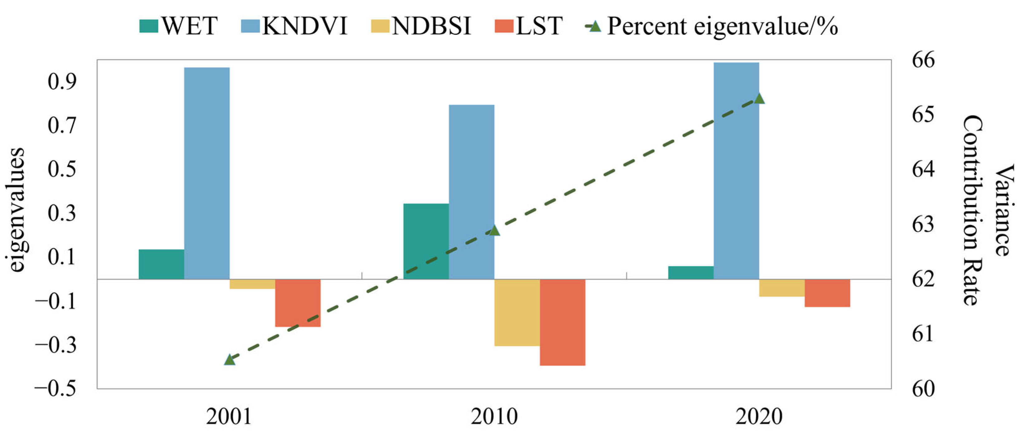
3.1. Results of Principal Component Analysis

Table 4 and Figure 4 present the results of the principal component analysis for four indicators over three typical years in the SNRC. The following characteristics can be observed from the table: (1) Three historical images from the years 2001, 2010, and 2020 were selected, where the contribution rates of the first principal component (PC1) were more than 60%, signifying that PC1 concentrated most of the characteristics of four component indices, so PC1 was utilized to construct the final RSEI; (2) From PC2 to PC4, the magnitude of the eigenvalues and the positive and negative values were both abnormal variable loads. (3) Upon analyzing the contribution rates of the four indicators to the RSEI, it is evident that in PC1, the eigenvalues of NDVI and WET were positive, indicating that NDVI and WET contributed to the enhancement of the ecological environment. Conversely, the eigenvalues of LST and NDBSI were negative, suggesting that they had inhibitory effects on ecological improvement. These findings align with the actual situation and previous research results [13,69].

3.2. Temporal and Spatial Evolution Characteristics of RSEI

From the time-series perspective, the annual mean values of the RSEI in the SNRC demonstrated an overall significant fluctuating upward trend from 2001 to 2020 (p < 0.05). As depicted in Figure 5d, upon analyzing the annual mean RSEI values for the growing season, it was observed that the RSEI underwent a growth rate of 0.84%/a over the twenty-year period, with a multi-year average of 0.626. The maximum value occurred in 2018 at 0.730, while the minimum value was observed in 2005 at 0.510. Temporally, the trend of the RSEI variation can be roughly divided into two phases, displaying a trend of “initial fluctuating decline, followed by significant improvement”. Specifically, from 2001 to 2005, there was a non-significant downward trend (p = 0.244) with a decline rate of −1.76%/a, followed by a significant increase with a growth rate of 0.55%/a from 2006 to 2020 (p < 0.05). In addition, the RSEI values of each prefecture and county underwent a statistical analysis. The RSEI values of HUT and HNT exhibited a significant upward trend, with the RSEI of HUT increasing from 0.503 in 2001 to 0.714 in 2020. The standard deviation of the RSEI series for HUT and HNT reached 0.125 and 0.131, surpassing the average level of 0.093, indicating significant fluctuations in the EEQ. The trend of RSEI values in GMC and YST displayed a similar pattern, showing a slight upward trend. The multi-year average of the RSEI in GMC was the lowest in the SNRC at 0.559, while the multi-year average of the RSEI in YST was 0.604. The RSEI values of GLT exhibited non-significant fluctuation, with no obvious trend. Survey data indicate that the ecological system of the SNRC has shown gradual improvement in recent years, which is attributed to the implementation of the First Phase Plans on Ecological Protection and Construction in Qinghai Sanjiangyuan (EPCQS I) from 2005 to 2012 and the Second Phase Plans on Ecological Protection and Construction in Qinghai Sanjiangyuan (EPCQS II) from 2013 to 2020. There has been a significant expansion in the area of lakes and wetlands, a rapid increase in forest and grass vegetation coverage, steady enhancement of water conservation capacity, and a continuous rise in the amount of water resources. The results of the survey data align with the changes in the RSEI obtained in this study.
From the spatial distribution perspective, the spatial pattern of the ecological conditions in the SNRC exhibited significant spatial heterogeneity. As depicted in Figure 5a–c, the ecological conditions improved from the northwest to the southeast, demonstrating an overall spatial pattern of “low in the west and high in the east”. Furthermore, Figure 5f,g illustrates the average of the RSEI and the spatial distribution for each autonomous prefecture and county in the SNRC. A comparative analysis of the RSEI values from 2001 to 2020 reveals significant spatial disparities among the autonomous prefectures, with the RSEI values ranking from high to low as follows: HUT, HNT, GLT, YST, and GMC. The Global Moran’s I was utilized to assess the correlation of the ecological environment in the SNRC. Based on the research results, with the significance level of the p-value set at 1%, the values of Global Moran’s I for different periods in the SNRC were consistently positive, and the average value of Global Moran’s I was 0.793, indicating that the spatial distribution pattern of the RSEI demonstrates clustering characteristics alongside significant spatial autocorrelation. To depict the spatial distribution pattern of the EEQ in the study area in a more intuitive manner, LISA clustering maps were generated. As depicted in Figure 5h, the EEQ of the SNRC consistently exhibited clustering characteristics in local spatial autocorrelation from 2001 to 2020. The spatial distribution pattern primarily manifested as “H-H” and “L-L” clustering, with the proportion of “H-H” clustering areas exceeding 35% and the proportion of “L-L” clustering areas exceeding 30%. The proportion of “H-H” clustering areas increased from 40.27% in 2001 to 52.17% in 2020, primarily concentrated in the southeast of HUT, HNT, the southeast of GLT, and the south of YST. Conversely, the proportion of “L-L” clustering areas decreased from 40.78% in 2001 to 30.85% in 2020, mainly distributed in GMC and the northwest and central parts of YST. The proportions of “H-L” and “L-H” areas were relatively small, both accounting for less than 5% and sporadically distributed.
According to Xu et al. [13], the EEQ of the SNRC was categorized into five levels based on the RSEI values: very poor (0–0.2), poor (0.2–0.4), moderate (0.4–0.6), good (0.6–0.8), and very good (0.8–1.0), as shown in Table 5. The areas with poor and very poor levels were relatively small, with the area of the very poor level being the smallest, accounting for less than 5% each year. In contrast, the areas with moderate and good levels constituted the largest portion, accounting for over 70% of the total area in the results of each year. Specifically, the area with a moderate level exhibited a trend of initial increase followed by decrease, while the area with a good level showed a consistent trend. Simultaneously, the area with a very good level gradually increased, reaching its peak in 2018 at 30.12%. The changes in areas with different levels were consistent with the trend of the RSEI in the SNRC over the past 20 years. By analyzing the EEQ level transfer matrix and Sankey diagram (Figure 6), it was observed that from 2000 to 2010 and from 2010 to 2020, 27.63% and 47.06% of the areas in the SNRC, respectively, underwent a transfer in EEQ levels. Apart from the areas where the level remained stable, the transfer from poor to very poor levels and from good to moderate and very good levels was notably pronounced. It was evident that the mutual transformation from moderate to good and very good levels was the primary factor influencing the annual variation of mean RSEI values. The increase in the proportion of areas classified as good and very good levels was primarily associated with the implementation of ecological protection projects in the Sanjiangyuan National Nature Reserve (SNNR).

3.3. EEQ Temporal Evolution

3.3.1. Time-Series Decomposition Results Based on STL

Using the STL decomposition to perform time-series decomposition on the monthly-scale RSEI, three component sequences of the RSEI were extracted to reveal their changing trends, periodic lengths, range of random fluctuations, and interconnections. Figure 7 presents the comparison of seasonal components, trend components, and remainder components obtained using the STL decomposition algorithm with the original data. It is evident that the trend component data curve obtained using the STL decomposition is smooth, indicating low-frequency changes. The Sen’s slope method revealed that the monthly-scale trend component increased at a rate of 0.038%/month, combined with the MMK trend test result (p < 0.05), signifying a significant upward trend in the trend component, which is the primary factor influencing the fluctuation in the mean RSEI. The seasonal component exhibits a high frequency of change, demonstrating a seasonal trend with an evident periodicity of 12 months. The variation aligns with the original data, displaying a strong correlation with the preceding period of data, indicating long-term dependence. The remainder component, obtained by subtracting the seasonal and trend components from the original RSEI data, encompasses some random noise or outliers in the data. Unlike the seasonal component sequence, the remainder component sequence does not exhibit obvious regularity, featuring unpredictable fluctuations and strong randomness. The degree of fluctuation in the remainder component in the latter half of the time-series surpasses that in the first half.

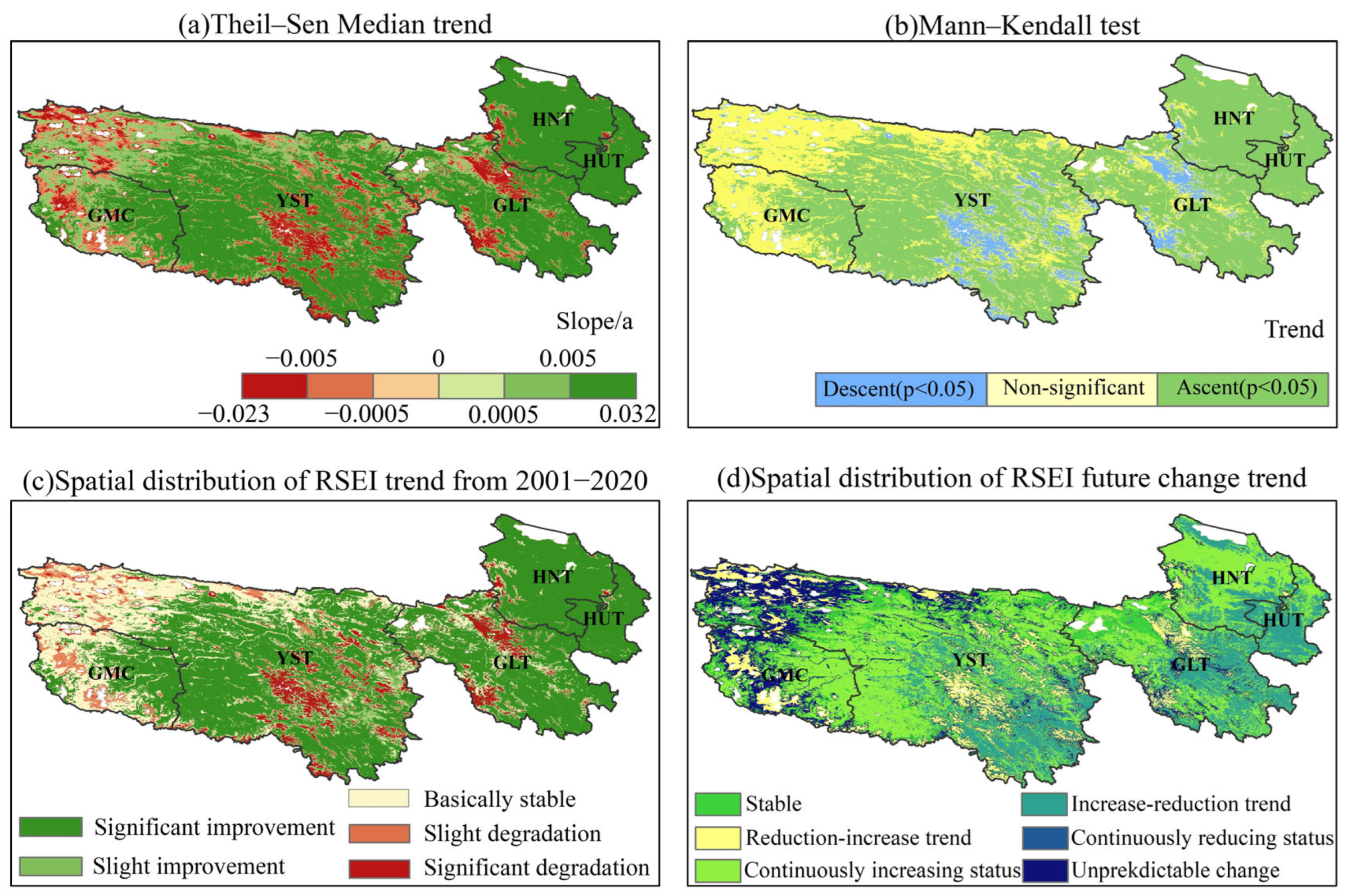
3.3.2. Change Trend and Sustainability Analysis of EEQ

After conducting the STL decomposition on the time-series data, the Theil–Sen slope estimator and MMK trend test were applied to the monthly-scale RSEI trend data from 2001 to 2020 at the pixel scale, and the results are depicted in Figure 8a,b. Based on Table 6, the RSEI trend was categorized into five levels based on the Sen’s slope, as illustrated in Figure 8c. The significance level of the RSEI is generally set at 0.05; when the absolute value of Z exceeds 1.96, the trend passes the significance test with confidence levels of 95%, indicating a statistically significant change. Notably, the significant improvement level represented the highest proportion of the area, accounting for 62.96%, predominantly concentrated in the northeastern part of GMC, the southern part of GLT, the HUT, and HNT. Subsequently, the area with a basically stable trend accounted for 23.37%, mainly distributed in the northwest of GMC and YST. The proportions of significantly degraded and slightly degraded areas were 6.31% and 5.07%, respectively. Significantly degraded areas were primarily distributed in the central part of YST, as well as the northeast and southwest of GLT. Slightly degraded areas were relatively scattered, mostly distributed in the western part of GMC and the northwest of YST. The proportion of slightly improved areas was minimal and scattered, accounting for less than 5%. According to the periodic comprehensive assessment report of ecological effectiveness of the National Development and Reform Commission of China [70], in recent years, the EEQ in the SNRC has demonstrated improvement, with a consolidation of ecological functions. The annual growth rate of water conservation capacity has exceeded 6%. Furthermore, there has been an increase of more than 11% in grassland coverage and a 30% increase in grass yield compared to a decade ago. These results align with the RSEI quality evolution trend obtained in this study.
The average HI of the RSEI time series from 2000 to 2020 was 0.51. The proportion of the area with a HI greater than 0.5 was 47.07%, indicating a weak positive continuity in the evolution of EEQ in the SNRC. Furthermore, combining the MMK trend test with the HI can predict the future trend of ecological quality in the SNRC. It can be inferred that the future trend of the RSEI is mainly characterized by anti-persistence, with the overall ecological environment improving while local degradation occurs. The results, as depicted in Table 7 and Figure 8d, indicate that the proportion of the areas where the EEQ will continue to improve in the future is the largest, reaching 33.74%. This improvement is mainly distributed in the east of GMC, the west of YST, the northwest of GLT, and the north of HNT. The second highest proportion is the areas that are anticipated to transition from improvement to degradation in the future, reaching 21.21%. These areas are distributed in the south of YST, the southeast of GLT, and the south of HNT. Additionally, 18.14% of the areas are projected to maintain continuous stability in the future, predominantly distributed in the northern part of YST and GLT. A total of 15.52% of the areas are anticipated to change unpredictably, primarily distributed in the western part of GMC and the northwestern part of YST. The area expected to undergo continuous degradation amounts to less than 5%, scattered throughout the region and in small quantities.

4. Discussion

4.1. SSA Time-Series Interpolation Accuracy Assessment

To verify the predictive accuracy of SSA time-series interpolation, remote sensing images of the MOD11A2 dataset from 2001 to 2020 were selected. A total of 18,466 sample points (1% of the total number of pixels) were randomly selected for interpolation from the complete monthly time-series data. Subsequently, SSA was employed to sequentially fill in 18,466 missing pixel values under scenarios with missing proportions of 0.1, 0.2, 0.3, 0.4, and 0.5. Accuracy testing and analyses were conducted through 10 iterations for each sample point, utilizing the original pixel values as the “true values” and the “fitted values” generated by the aforementioned interpolation framework. The average value and standard deviation (STD) of the coefficient of determination (R2), Mean Absolute Error (MAE), and Root Mean Square Error (RMSE) after 10 iterations were computed as the accuracy evaluation metrics for each sample point. The R2 is calculated as 1.0 minus the ratio of the regression sum of squares (SSregression) to the sum of all squares (SStotal). Additionally, the study compared the prediction results of the commonly used linear interpolation (LI) [71] and cubic spline interpolation (CSI) [72] methods with the SSA time-series interpolation. The analysis of Table 8 reveals a progressive decrease in the R2 as the proportion of missing data escalates, accompanied by a corresponding gradual increase in the MAE and RMSE. The difference between the average values of the R2 obtained using SSA and LI is at most 0.13; while CSI yields the smallest average R2 values, the maximum difference in average values of R2 between SSA and CSI can be as high as 0.31. Furthermore, the average values of MAE obtained using SSA generally fall below 100 and can be as much as 25.79% lower than the average MAE obtained using LI, and 36.06% lower than the average MAE obtained using CSI. In summary, the results of the three accuracy evaluation metrics for the predicted values generated using SSA time-series interpolation all surpass those of LI and CSI. Consequently, the SSA time-series interpolation effectively enhances the interpolation accuracy, yielding fitted signals closely aligned with real surface ecological conditions.

4.2. Effectiveness Evaluation of Filtering Methods

To assess the effectiveness of the filtering methods within the data reconstruction framework, this study employed three distinct ways for denoising and smoothing the four indicators: WS, Savitzky–Golay (SG) filtering [73], Double Logistic (DL) filtering, [74] and without filtering (w/o). The SG filtering method is a polynomial fitting method curve based on local features, in which a simplified least square fitting convolution is used to determine the weighting coefficients and produce the weighted mean in a moving window. On the other hand, DL filtering is a semi-local fitting method that divides the values corresponding to time points in the entire time series into multiple intervals based on their maximum or minimum values and performs local fitting on these intervals using double logistic functions. The reconstructed RSEI sequences and variance contribution rates were derived through PCA, and the comparative results are depicted in Figure 9. As illustrated in the figure, compared to the other three ways, the variance contribution rate obtained after applying the WS method produced a smoother curve, effectively filtering out image noise. In contrast, the variance contribution rate curve obtained from SG filtering exhibited significant fluctuations and a jagged phenomenon, merely removing noise points in the time-series data from a data perspective. The curve resulting from the DL method is relatively smooth, with the lowest mean variance contribution rate. The variance contribution rate curve obtained through the w/o method displayed a fluctuating trend characterized by a jagged phenomenon, numerous noise, and outlier values. Additionally, the comparative analysis of the mean RSEI values obtained from the four ways reveals that the mean value of the RSEI after WS processing exhibited substantial fluctuations, demonstrating an overall upward trend with a multi-year average of 0.626. The trend of mean RSEI values after DL method is relatively consistent with the trend of the RSEI after WS processing, with a multi-year average of 0.604. Compared to WS processing, the mean value of the RSEI after SG filtering exhibited comparatively smaller fluctuations, displaying a gradual increasing trend over twenty years, with a growth rate of 0.04%/a and a multi-year average of 0.572. Conversely, the curve illustrating the mean value of the RSEI obtained through w/o appeared smoother, indicating an initial decrease followed by an upward trend with a multi-year average of 0.515. Therefore, the results of WS are favorable as they meet the requirements for filtering out noise and outliers in time-series data without exhibiting an obvious jagged phenomenon.

4.3. Spatial and Temporal Distribution of RSEI

To further explore the spatio-temporal distribution patterns of the RSEI, this study integrated land cover data of the SNRC, as depicted in Figure 10a, to investigate the correlation between the distribution of the RSEI and the land use patterns. The western part of the SNRC generally exhibits altitudes exceeding 4000 m, mainly consisting of bare rocks, bare soil, and sparse grassland, with minimal anthropogenic influence. The cold and harsh environment restricts vegetation productivity, resulting in suboptimal ecological conditions and low RSEI values, mainly characterized by “L-L” clustering. The central and eastern parts of the SNRC are predominantly covered by grasslands, characterized by greater vegetation coverage and enhanced ecological quality, consequently yielding higher RSEI values, mainly exhibiting a “H-H” spatial distribution pattern. The southern and eastern parts of the SNRC have limited forested areas. The EEQ of the southern forest is improving, but the EEQ of the eastern forest is partially degrading. The RSEI primarily demonstrates an “L-L” clustering pattern, with sporadic instances of “L-H” and “H-L” spatial distributions. This is possibly attributed to residential and cultivated land in the eastern forest, indicating that human activities are influencing the trend of EEQ improvement. In general, areas with poor ecological conditions within the study area predominantly coincide with population agglomerations, cultivated land, unutilized land, and bare ground, suggesting a notable influence of human production activities and vegetation coverage on the EEQ. Additionally, the SNRC is characterized by a dense network of rivers and numerous lakes. Figure 10c illustrates that the RSEI texture at river confluences reflects the directional flow and distribution of the rivers. Furthermore, the spatio-temporal distribution of the RSEI alters in correspondence with the distribution of mountain ranges and variations in terrain, displaying a distinct topographical distribution.

4.4. Limitations of RSEI

The use of the RSEI still presents some limitations. Firstly, the application of the model has a high degree of arbitrariness, making it difficult to be uniformly applied [75,76]. Additionally, the lack of a fixed standard for the contribution value of PC1 makes it difficult to guarantee a high contribution rate and low data loss rate [77]. Relying solely on PC1 as an ecological evaluation index may result in the loss of detailed information [78]. Secondly, similar to other RSEI studies [79,80], water bodies are masked out, limiting the assessment to land surfaces and leading to the inability to fully consider the ecological benefits of water bodies to the surrounding environment. Thirdly, this study also has certain limitations in the evaluation of EEQ, as it only considers the impact of surface factors on EEQ while neglecting the influence of other factors. Therefore, the incorporation of diverse spatial data, such as land use patterns [81], dynamic carbon storage [82], and full element considerations [83], can provide a more comprehensive understanding of the ecosystem. Integrating these additional variables will contribute to a more comprehensive and holistic assessment of EEQ.

5. Conclusions

This study proposes a complete high-quality framework for MODIS time-series data reconstruction, which is utilized to construct the RSEI sequence of the SNRC spanning from 2001 to 2020, facilitating the observation of spatio-temporal dynamic changes and the evolution trends in EEQ. The primary conclusions are as follows:
The RSEI values of the SNRC exhibited a trend of “initial fluctuating decline, followed by significant improvement”, with a multi-year average of 0.626. The EEQ was dominated by moderate and good levels, with the sum of the area proportions exceeding 70% in the results of each year.
The spatial pattern of the EEQ demonstrated significant spatial heterogeneity, featuring a distinct “low in the west and high in the east” pattern. The spatial distribution pattern of the RSEI exhibited clustering characteristics alongside significant spatial autocorrelation. Local autocorrelation primarily manifested as “high-high” and “low-low” clusters. The presence of poor ecological conditions is primarily linked to population agglomerations, cultivated land, unutilized land, and bare ground, whereas grasslands and forests demonstrate higher RSEI values.
The result of the trend analysis showed a significant trend in RSEI variation, mainly characterized by an improvement trend, accounting for 62.96%, with 6.31% still showing significant degradation. The HI results indicated that the future RSEI trend is predominantly anti-persistent, with 33.74% of the area projected to continue improving in EEQ, while 21.21% is expected to transition from improvement to degradation.
Based on the aforementioned conclusions, it is evident that the ecological system in the SNRC has gradually improved in recent years, leading to enhanced EEQ and strengthened ecological functions. The ecological protection and construction projects in the SNRC have yielded remarkable results. Furthermore, the reconstructed RSEI effectively eliminates outliers’ influence and obtains reliable MODIS data, indicating that the high-quality framework for MODIS time-series data reconstruction constructed in this study exhibits strong data stability and robustness, rendering it suitable for the continuous monitoring of EEQ over a long time series and large-scale regions.

Author Contributions

Data curation, X.X. and Y.Z.; methodology, X.X.; resources, Y.C.; software, X.X., Y.C., and M.H.; writing—original draft, X.X.; writing—review and editing, H.L. All authors have read and agreed to the published version of the manuscript.

Funding

This research was funded by National Natural Science Foundation of China, grant number 41501291.

Institutional Review Board Statement

Not applicable.

Informed Consent Statement

Not applicable.

Data Availability Statement

The data presented in this study are available on request from the corresponding author.

Acknowledgments

The authors sincerely thank the editors and anonymous reviewers for their kind view and constructive suggestions.

Conflicts of Interest

The authors declare no conflicts of interest.

References

  1. Ji, P.; Yuan, X. High-resolution land surface modeling of hydrological changes over the Sanjiangyuan region in the eastern Tibetan Plateau: 2. Impact of climate and land cover change. J. Adv. Model. Earth Syst. 2018, 10, 2829–2843. [Google Scholar] [CrossRef]
  2. Chen, W.; Huang, H.; Tian, Y.; Du, Y. Monitoring and assessment of the eco-environment quality in the Sanjiangyuan region based on Google Earth Engine. J. Geo-Inf. Sci. 2019, 21, 1382–1391. [Google Scholar] [CrossRef]
  3. Liu, D.; Cao, C.; Dubovyk, O.; Tian, R.; Chen, W.; Zhuang, Q.; Zhao, Y.; Menz, G. Using fuzzy analytic hierarchy process for spatio-temporal analysis of eco-environmental vulnerability change during 1990–2010 in Sanjiangyuan region, China. Ecol. Indic. 2017, 73, 612–625. [Google Scholar] [CrossRef]
  4. Tang, H.; Xiao, F.; Zhang, Q.; Shi, J. Vegetation change and its response to climate change in Three-River Source Region. Adv. Clim. Chang. Res. 2006, 2, 177–180. [Google Scholar] [CrossRef]
  5. Li, L.; Zhu, X.; Zhou, L.; Wang, Q. Climatic changes over headwater of the Three-River-Area and its effect on ecological environment. Meteorol. Mon. 2004, 30, 18–21. [Google Scholar] [CrossRef]
  6. Zhai, X.; Liang, X.; Yan, C.; Xing, X.; Jia, H.; Wei, X.; Feng, K. Vegetation dynamic changes and their response to ecological engineering in the Sanjiangyuan Region of China. Remote Sens. 2020, 12, 4035. [Google Scholar] [CrossRef]
  7. Ma, T.; Swallow, B.; Zhong, L.; Xu, K.; Sang, W.; Jia, L. Local perspectives on social-ecological transformation: China’s Sanjiangyuan National Park. Environ. Dev. Sustain. 2024, 26, 1809–1829. [Google Scholar] [CrossRef]
  8. Zhai, X.; Yan, C.; Xing, X.; Jia, H.; Wei, X.; Feng, K. Spatial-temporal changes and driving forces of aeolian desertification of grassland in the Sanjiangyuan region from 1975 to 2015 based on the analysis of Landsat images. Environ. Monit. Assess. 2021, 193, 2. [Google Scholar] [CrossRef]
  9. Bingrong, Z.; Shengcui, Z.; Hongmei, L. Temporal and spatial characteristics of vegetation net primary productivity and its responses to climate change in Three-River Headwaters region. J. Arid. Meteorol. 2016, 34, 958. [Google Scholar] [CrossRef]
  10. McGregor, G.R. Climate variability and change in the Sanjiangyuan region. In Landscape and Ecosystem Diversity, Dynamics and Management in the Yellow River Source Zone; Springer: Berlin/Heidelberg, Germany, 2016; pp. 35–57. [Google Scholar] [CrossRef]
  11. Xu, Y.; Zhou, H. A preliminary study on advances in assessment of eco-environmental quality in China. Arid. Land Geogr. 2003, 26, 166–172. [Google Scholar] [CrossRef]
  12. Karbalaei Saleh, S.; Amoushahi, S.; Gholipour, M. Spatiotemporal ecological quality assessment of metropolitan cities: A case study of central Iran. Environ. Monit. Assess. 2021, 193, 305. [Google Scholar] [CrossRef] [PubMed]
  13. Xu, H. A remote sensing urban ecological index and its application. Acta Ecol. Sin 2013, 33, 7853–7862. [Google Scholar]
  14. Xiong, Y.; Xu, W.; Lu, N.; Huang, S.; Wu, C.; Wang, L.; Dai, F.; Kou, W. Assessment of spatial–temporal changes of ecological environment quality based on RSEI and GEE: A case study in Erhai Lake Basin, Yunnan province, China. Ecol. Indic. 2021, 125, 107518. [Google Scholar] [CrossRef]
  15. Wen, X.; Ming, Y.; Gao, Y.; Hu, X. Dynamic monitoring and analysis of ecological quality of pingtan comprehensive experimental zone, a new type of sea island city, based on RSEI. Sustainability 2019, 12, 21. [Google Scholar] [CrossRef]
  16. Naseri, N.; Mostafazadeh, R. Spatial relationship of Remote Sensing Ecological Indicator (RSEI) and landscape metrics under urban development intensification. Earth Sci. Inf. 2023, 16, 3797–3810. [Google Scholar] [CrossRef]
  17. Yao, K.; Halike, A.; Chen, L.; Wei, Q. Spatiotemporal changes of eco-environmental quality based on remote sensing-based ecological index in the Hotan Oasis, Xinjiang. J. Arid. Land 2022, 14, 262–283. [Google Scholar] [CrossRef]
  18. Ren, K.; Luo, M.; Zhao, Y.; Han, L.; Zhang, L.; Yang, S. Evaluation of ecological environment and urban development quality in Xi’an City, China. J. Appl. Ecol. 2022, 33, 2485–2492. [Google Scholar] [CrossRef]
  19. Yuan, W.; Yuhao, Z.; Jiansheng, W. Dynamic monitoring of long time series of ecological quality in urban agglomerations using Google Earth Engine cloud computing: A case study of the Guangdong-Hong Kong-Macao Greater Bay Area, China. Acta Ecol. Sin. 2020, 40, 8461–8473. [Google Scholar] [CrossRef]
  20. Wang, J.; Zhao, M.; Li, J.B.; Zhen, C. Dynamic monitoring and driving forces of eco-environmental quality in the Qinba Mountains based on MODIS timeseries data. Mt. Res. 2021, 39, 830. [Google Scholar] [CrossRef]
  21. Yang, X.; Meng, F.; Fu, P.; Wang, Y.; Liu, Y. Time-frequency optimization of RSEI: A case study of Yangtze River Basin. Ecol. Indic. 2022, 141, 109080. [Google Scholar] [CrossRef]
  22. Ji, J.; Wang, S.; Zhou, Y.; Liu, W.; Wang, L. Spatiotemporal change and landscape pattern variation of eco-environmental quality in Jing-Jin-Ji urban agglomeration from 2001 to 2015. IEEE Access 2020, 8, 125534–125548. [Google Scholar] [CrossRef]
  23. Wei, J.; Sun, L.; Peng, Y.; Wang, L.; Zhang, Z.; Bilal, M.; Ma, Y. An improved high-spatial-resolution aerosol retrieval algorithm for MODIS images over land. J. Geophys. Res. Atmos. 2018, 123, 12291–12307. [Google Scholar] [CrossRef]
  24. Zhao, Z.; Gao, L.; Chen, D.; Yue, A.; Chen, J.; Liu, D.; Yang, J.; Meng, Y. Development of satellite remote sensing and image processing platform. J. Image Graph. 2019, 24, 2098–2110. [Google Scholar] [CrossRef]
  25. Hird, J.N.; McDermid, G.J. Noise reduction of NDVI time series: An empirical comparison of selected techniques. Remote Sens. Environ. 2009, 113, 248–258. [Google Scholar] [CrossRef]
  26. Miao, W.; Chen, Y.; Kou, W.; Lai, H.; Sazal, A.; Wang, J.; Li, Y.; Hu, J.; Wu, Y.; Zhao, T. The HANTS-fitted RSEI constructed in the vegetation growing season reveals the spatiotemporal patterns of ecological quality. Sci. Rep. 2024, 14, 14686. [Google Scholar] [CrossRef]
  27. Liu, R.; Shang, R.; Liu, Y.; Lu, X. Global evaluation of gap-filling approaches for seasonal NDVI with considering vegetation growth trajectory, protection of key point, noise resistance and curve stability. Remote Sens. Environ. 2017, 189, 164–179. [Google Scholar] [CrossRef]
  28. Zheng, Z.; Wu, Z.; Chen, Y.; Guo, C.; Marinello, F. Instability of remote sensing based ecological index (RSEI) and its improvement for time series analysis. Sci. Total Environ. 2022, 814, 152595. [Google Scholar] [CrossRef] [PubMed]
  29. Wu, X.; Shen, C.; Shi, L.; Wan, Y.; Ding, J.; Wen, Q. Spatio-temporal evolution characteristics and simulation prediction of carbon storage: A case study in Sanjiangyuan Area, China. Ecol. Inf. 2024, 80, 102485. [Google Scholar] [CrossRef]
  30. Duan, X.; Chen, Y.; Wang, L.; Zheng, G.; Liang, T. The impact of land use and land cover changes on the landscape pattern and ecosystem service value in Sanjiangyuan region of the Qinghai-Tibet Plateau. J. Environ. Manag. 2023, 325, 116539. [Google Scholar] [CrossRef]
  31. Savtchenko, A.; Ouzounov, D.; Ahmad, S.; Acker, J.; Leptoukh, G.; Koziana, J.; Nickless, D. Terra and Aqua MODIS products available from NASA GES DAAC. Adv. Space Res. 2004, 34, 710–714. [Google Scholar] [CrossRef]
  32. Zeng, L.; Wardlow, B.D.; Hu, S.; Zhang, X.; Zhou, G.; Peng, G.; Xiang, D.; Wang, R.; Meng, R.; Wu, W. A novel strategy to reconstruct NDVI time-series with high temporal resolution from MODIS multi-temporal composite products. Remote Sens. 2021, 13, 1397. [Google Scholar] [CrossRef]
  33. Shao, Q.; Liu, S.; Ning, J.; Liu, G.; Yang, F.; Zhang, X.; Niu, L.; Huang, H.; Fan, J.; Liu, J. Assessment of ecological benefits of key national ecological projects in China in 2000–2019 using remote sensing. Acta Geogr. Sin. 2022, 77, 2133–2153. [Google Scholar] [CrossRef]
  34. Dong, C.; Zhao, G. Influence of time series data quality on land cover classification accuracy. Remote Sens. Technol. Appl. 2020, 35, 558–566. [Google Scholar]
  35. Zhou, M.; Shen, R.; Chen, J. Filtering and reconstruction of LAI time series data by SG filter based on pixel quality analysis and outlier detection. Remote Sens. Technol. Appl. 2019, 34, 323–330. [Google Scholar]
  36. Xu, H. A new index for delineating built-up land features in satellite imagery. Int. J. Remote Sens. 2008, 29, 4269–4276. [Google Scholar] [CrossRef]
  37. Xu, H.; Wang, Y.; Guan, H.; Shi, T.; Hu, X. Detecting ecological changes with a remote sensing based ecological index (RSEI) produced time series and change vector analysis. Remote Sens. 2019, 11, 2345. [Google Scholar] [CrossRef]
  38. Guo, D.; Wang, C.; Zang, S.; Hua, J.; Lv, Z.; Lin, Y. Gap-Filling of 8-Day Terra MODIS daytime land surface temperature in high-latitude cold region with generalized additive models (GAM). Remote Sens. 2021, 13, 3667. [Google Scholar] [CrossRef]
  39. Camps-Valls, G.; Campos-Taberner, M.; Moreno-Martínez, Á.; Walther, S.; Duveiller, G.; Cescatti, A.; Mahecha, M.D.; Muñoz-Marí, J.; García-Haro, F.J.; Guanter, L. A unified vegetation index for quantifying the terrestrial biosphere. Sci. Adv. 2021, 7, eabc7447. [Google Scholar] [CrossRef]
  40. Zhang, L.; Ren, X.; Wang, J.; He, H.; Wang, S.; Wang, M.; Piao, S.; Yan, H.; Ju, W.; Gu, F. Interannual variability of terrestrial net ecosystem productivity over China: Regional contributions and climate attribution. Environ. Res. Lett. 2019, 14, 014003. [Google Scholar] [CrossRef]
  41. Lu, J.; Carbone, G.J.; Gao, P. Detrending crop yield data for spatial visualization of drought impacts in the United States, 1895–2014. Agric. For. Meteorol. 2017, 237, 196–208. [Google Scholar] [CrossRef]
  42. Ols, C.; Klesse, S.; Girardin, M.P.; Evans, M.E.; DeRose, R.J.; Trouet, V. Detrending climate data prior to climate–growth analyses in dendroecology: A common best practice? Dendrochronologia 2023, 79, 126094. [Google Scholar] [CrossRef]
  43. De Beurs, K.; Henebry, G. A statistical framework for the analysis of long image time series. Int. J. Remote Sens. 2007, 26, 1551–1573. [Google Scholar] [CrossRef]
  44. Okkaoğlu, Y.; Akdi, Y.; Ünlü, K.D. Daily PM10, periodicity and harmonic regression model: The case of London. Atmos. Environ. 2020, 238, 117755. [Google Scholar] [CrossRef]
  45. Pan, N.; Feng, X.; Fu, B.; Wang, S.; Ji, F.; Pan, S. Increasing global vegetation browning hidden in overall vegetation greening: Insights from time-varying trends. Remote Sens. Environ. 2018, 214, 59–72. [Google Scholar] [CrossRef]
  46. Allen, D.P. A frequency domain Hampel filter for blind rejection of sinusoidal interference from electromyograms. J. Neurosci. Methods 2009, 177, 303–310. [Google Scholar] [CrossRef]
  47. Salem, O.; Liu, Y.; Mehaoua, A. A lightweight anomaly detection framework for medical wireless sensor networks. In Proceedings of the 2013 IEEE Wireless Communications and Networking Conference (WCNC), Shanghai, China, 7–10 April 2013; pp. 4358–4363. [Google Scholar]
  48. Pearson, R.K.; Neuvo, Y.; Astola, J.; Gabbouj, M. Generalized hampel filters. EURASIP J. Adv. Signal Process. 2016, 2016, 87. [Google Scholar] [CrossRef]
  49. Colebrook, J. Continuous plankton records-zooplankton and environment, northeast Atlantic and North-Sea, 1948–1975. Oceanol. Acta 1978, 1, 9–23. [Google Scholar]
  50. Zeng, C.; Long, D.; Shen, H.; Wu, P.; Cui, Y.; Hong, Y. A two-step framework for reconstructing remotely sensed land surface temperatures contaminated by cloud. ISPRS J. Photogramm. Remote Sens. 2018, 141, 30–45. [Google Scholar] [CrossRef]
  51. Ghafarian Malamiri, H.R.; Rousta, I.; Olafsson, H.; Zare, H.; Zhang, H. Gap-filling of MODIS time series land surface temperature (LST) products using singular spectrum analysis (SSA). Atmosphere 2018, 9, 334. [Google Scholar] [CrossRef]
  52. Eilers, P.H. A perfect smoother. Anal. Chem. 2003, 75, 3631–3636. [Google Scholar] [CrossRef]
  53. Wang, Q.; Moreno-Martínez, Á.; Muñoz-Marí, J.; Campos-Taberner, M.; Camps-Valls, G. Estimation of vegetation traits with kernel NDVI. ISPRS J. Photogramm. Remote Sens. 2023, 195, 408–417. [Google Scholar] [CrossRef]
  54. Cleveland, R.B.; Cleveland, W.S.; McRae, J.E.; Terpenning, I. STL: A seasonal-trend decomposition. J. Off. Stat 1990, 6, 3–73. [Google Scholar]
  55. Cleveland, W.S.; Devlin, S.J. Locally weighted regression: An approach to regression analysis by local fitting. J. Am. Stat. Assoc. 1988, 83, 596–610. [Google Scholar] [CrossRef]
  56. Sen, P.K. Estimates of the regression coefficient based on Kendall’s tau. J. Am. Stat. Assoc. 1968, 63, 1379–1389. [Google Scholar] [CrossRef]
  57. Kendall, M. Rank correlation methods. Biometrika 1948, 44, 298. [Google Scholar] [CrossRef]
  58. Mann, H.B. Nonparametric tests against trend. Econom. J. Econom. Soc. 1945, 13, 245–259. [Google Scholar] [CrossRef]
  59. Yue, S.; Wang, C. The Mann-Kendall test modified by effective sample size to detect trend in serially correlated hydrological series. Water Resour. Manag. 2004, 18, 201–218. [Google Scholar] [CrossRef]
  60. Yang, Z.; Tian, J.; Li, W.; Su, W.; Guo, R.; Liu, W. Spatio-temporal pattern and evolution trend of ecological environment quality in the Yellow River Basin. Acta Ecol. Sin. 2021, 41, 7627–7636. [Google Scholar] [CrossRef]
  61. Matalas, N.C.; Langbein, W. Information content of the mean. J. Geophys. Res. 1962, 67, 3441–3448. [Google Scholar] [CrossRef]
  62. Hurst, H.E. Long-term storage capacity of reservoirs. Trans. Am. Soc. Civ. Eng. 1951, 116, 770–799. [Google Scholar] [CrossRef]
  63. Long, Y.; Jiang, F.; Deng, M.; Wang, T.; Sun, H. Spatial-temporal changes and driving factors of eco-environmental quality in the Three-North region of China. J. Arid. Land 2023, 15, 231–252. [Google Scholar] [CrossRef]
  64. Peng, J.; Liu, Z.; Liu, Y.; Wu, J.; Han, Y. Trend analysis of vegetation dynamics in Qinghai–Tibet Plateau using Hurst Exponent. Ecol. Indic. 2012, 14, 28–39. [Google Scholar] [CrossRef]
  65. Boori, M.S.; Choudhary, K.; Paringer, R.; Kupriyanov, A. Spatiotemporal ecological vulnerability analysis with statistical correlation based on satellite remote sensing in Samara, Russia. J. Environ. Manag. 2021, 285, 112138. [Google Scholar] [CrossRef]
  66. Griffith, D.A. Spatial autocorrelation. In Handbook of Applied Spatial Analysis; Springer: Berlin/Heidelberg, Germany, 1987. [Google Scholar] [CrossRef]
  67. Anselin, L. Local indicators of spatial association—LISA. Geogr. Anal. 1995, 27, 93–115. [Google Scholar] [CrossRef]
  68. Liu, Q.; Yu, F.; Mu, X. Evaluation of the ecological environment quality of the Kuye River source basin using the remote sensing ecological index. Int. J. Environ. Res. Public Health 2022, 19, 12500. [Google Scholar] [CrossRef] [PubMed]
  69. Zhang, Y.; She, J.; Long, X.; Zhang, M. Spatio-temporal evolution and driving factors of eco-environmental quality based on RSEI in Chang-Zhu-Tan metropolitan circle, central China. Ecol. Indic. 2022, 144, 109436. [Google Scholar] [CrossRef]
  70. Yaquan, D.; Ya, L.; Youjun, H. Charging Principle and Mode Selection of National Park Tickets in China. J. Beijing For. Univ. (Soc. Sci.) 2023, 22, 25–31. [Google Scholar] [CrossRef]
  71. Terry, W.; Lee, J.; Kumar, A. Time series analysis in acid rain modeling: Evaluation of filling missing values by linear interpolation. Atmos. Environ. 1986, 20, 1941–1943. [Google Scholar] [CrossRef]
  72. McKinley, S.; Levine, M. Cubic spline interpolation. Coll. Redw. 1998, 45, 1049–1060. [Google Scholar]
  73. Savitzky, A.; Golay, M.J. Smoothing and differentiation of data by simplified least squares procedures. Anal. Chem. 1964, 36, 1627–1639. [Google Scholar] [CrossRef]
  74. Beck, P.S.; Atzberger, C.; Høgda, K.A.; Johansen, B.; Skidmore, A.K. Improved monitoring of vegetation dynamics at very high latitudes: A new method using MODIS NDVI. Remote Sens. Environ. 2006, 100, 321–334. [Google Scholar] [CrossRef]
  75. Wu, Z.; Wang, M.; Chen, S.; Zou, D. Monitoring and evaluation of ecological environments spatio-temporal variation in mine based on RSEI a case of Yongding mine. Ecol. Sci. 2016, 35, 200. [Google Scholar] [CrossRef]
  76. Yang, X.; Meng, F.; Fu, P.; Zhang, Y.; Liu, Y. Spatiotemporal change and driving factors of the Eco-Environment quality in the Yangtze River Basin from 2001 to 2019. Ecol. Indic. 2021, 131, 108214. [Google Scholar] [CrossRef]
  77. Cheng, L.-L.; Wang, Z.-W.; Tian, S.-F.; Liu, Y.-T.; Sun, M.-Y.; Yang, Y.-M. Evaluation of eco-environmental quality in Mentougou District of Beijing based on improved remote sensing ecological index. Chin. J. Ecol. 2021, 40, 1177. [Google Scholar] [CrossRef]
  78. Song, M.; Luo, Y.; Duan, L. Evaluation of ecological environment in the Xilin Gol steppe based on modified remote sensing ecological index model. Arid. Zone Res. 2019, 36, 1521. [Google Scholar] [CrossRef]
  79. Hu, X.; Xu, H. A new remote sensing index for assessing the spatial heterogeneity in urban ecological quality: A case from Fuzhou City, China. Ecol. Indic. 2018, 89, 11–21. [Google Scholar] [CrossRef]
  80. Mostafiz, C.; Chang, N.-B. Tasseled cap transformation for assessing hurricane landfall impact on a coastal watershed. Int. J. Appl. Earth Obs. Geoinf. 2018, 73, 736–745. [Google Scholar] [CrossRef]
  81. Deng, Y.; Wang, S.; Bai, X.; Luo, G.; Wu, L.; Chen, F.; Wang, J.; Li, C.; Yang, Y.; Hu, Z. Vegetation greening intensified soil drying in some semi-arid and arid areas of the world. Agric. For. Meteorol. 2020, 292, 108103. [Google Scholar] [CrossRef]
  82. Yang, Y.; Li, H.; Qian, C. Analysis of the implementation effects of ecological restoration projects based on carbon storage and eco-environmental quality: A case study of the Yellow River Delta, China. J. Environ. Manag. 2023, 340, 117929. [Google Scholar] [CrossRef] [PubMed]
  83. Wang, Z.; Chen, T.; Zhu, D.; Jia, K.; Plaza, A. RSEIFE: A new remote sensing ecological index for simulating the land surface eco-environment. J. Environ. Manag. 2023, 326, 116851. [Google Scholar] [CrossRef] [PubMed]
Figure 1. Map of the SNRC. The abbreviations for each city and state in the figure are as follows: Golmud City (GMC), Yushu Tibetan Autonomous Prefecture (YST), Guoluo Tibetan Autonomous Prefecture (GLT), Hainan Tibetan Autonomous Prefecture (HNT), and Huangnan Tibetan Autonomous Prefecture (HUT). The basic geographic information was obtained from the National Catalogue Service for Geographic Information of China, while the vector boundary data of the SNRC were sourced from the National Ecological Science Data Center. Additionally, the digital elevation model (DEM) data used in this figure were provided by the US Geological Survey (USGS). The figure was produced using ArcGIS 10.8.
Sustainability 16 06231 g001
Figure 2. Technology roadmap. The abbreviations in the figure are as follows: normalized difference impervious surface index (NDBSI), wetness (WET), land surface temperature (LST), kernel normalized difference vegetation index (kNDVI), Seasonal-Trend Decomposition Procedure based on Loess (STL), and the first principal component (PC1). The figure was produced using ArcGIS 10.8 and Visio 2021.
Sustainability 16 06231 g002
Figure 3. Missing image statistics. The figure was produced by ArcGIS 10.8.
Sustainability 16 06231 g003
Figure 4. The first principal component (PC1) of four indicators (WET, KNDVI, LST, NDBSI) and their contribution rates in 2001, 2010, and 2020 respectively. The figure was produced using Origin 2022.
Sustainability 16 06231 g004
Figure 5. Characterization of RSEI spatio-temporal variations. Figures (ac), respectively, show the spatial distribution of EEQ levels in 2001, 2010, and 2020, which are categorized into five levels: very good, good, moderate, poor, and very poor. In Figure (d), MAX and MIN represent the maximum and minimum values of the annual-scale RSEI within the study area, while MEAN denotes the mean value of the annual-scale RSEI. Figure (e) displays the multi-year EEQ levels within the study area, and Figures (f,g) present the average RSEI values for each county and autonomous prefecture/city. Figure (h) shows the Moran’s I value for each year and the LISA clustering map of RSEI. The figure was produced using ArcGIS 10.8.
Sustainability 16 06231 g005aSustainability 16 06231 g005b
Figure 6. Sankey diagram of EEQ level transfer matrix from 2001 to 2020 (103 km2). The figure was produced using Python 3.9.
Sustainability 16 06231 g006
Figure 7. Schematic diagram of STL decomposition results of monthly RSEI time series from 2001 to 2020. The figure was produced using Origin 2022.
Sustainability 16 06231 g007
Figure 8. The law of quality evolution. Figures (ac) show the results of Theil–Sen median trend and MMK trend test of RSEI from 2001 to 2020 as well as the spatial distribution of the five categories of the RSEI trend. Figure (d) shows the spatial distribution of the six categories of the future trend of RSEI obtained by combining with the Hurst exponent. The figure was produced using ArcGIS 10.8.
Sustainability 16 06231 g008
Figure 9. The ratio of the variance contribution rate and the mean RSEI in the three cases. The figure was produced by Origin 2022.
Sustainability 16 06231 g009
Figure 10. Spatial and temporal distribution of RSEI. (a,b) show the land cover data of SNRC and the corresponding mean RSEI values of different land types, respectively; (c) shows the texture details of the mean RSEI image of typical areas. I, II, III represent three typical landform types respectively. The figure was produced using ArcGIS 10.8.
Sustainability 16 06231 g010
Table 1. Data sources and detailed descriptions of study.
Data
Collection
BandsDescriptionWavelengthTime
Resolution
Spatial ResolutionSource
MOD09A1v061RedSurface reflectance620–670 nm8 d500 mU.S. Geological Survey (USGS) and used in the GEE cloud computing platform
https://developers.google.com
(accessed on 16 May 2023)
NIR1841–876 nm
Blue459–479 nm
Green545–565 nm
NIR21230–1250 nm
SWIR11628–1652 nm
SWIR22105–2155 nm
MOD11A2v061LST_Day_
1 km
Day land surface temperature 8 d1000 m
MOD13A1v061sur_refl_b01Vegetation index (VI)645 nm16 d500 m
sur_refl_b02858 nm
Public version of basic geographic information N/A1:1 millionNational Catalogue Service for Geographic Information of China
https://www.webmap.cn/
(accessed on 22 May 2023)
Boundary data of the SNRC N/A1:1 millionNational Ecological Science
Data Center
http://www.nesdc.org.cn
(accessed on 22 May 2023)
SRTM3 N/A90 mGeospatial Data Cloud
https://www.gscloud.cn/
(accessed on 25 May 2023)
Table 2. Description of MODIS data.
Data
Collection
Number of
Images
Calculation
Bands
Index
MOD09A1920Red, Green, Blue,
NIR1, NIR2,
SWIR1, SWIR2
Normalized difference
impervious surface
index (NDBSI) [36]
Wetness (WET) [37]
MOD11A2920LST_Day_1kmLand surface
temperature (LST) [38]
MOD13A1460Red, NIR1kernel normalized difference
vegetation index (kNDVI) [39]
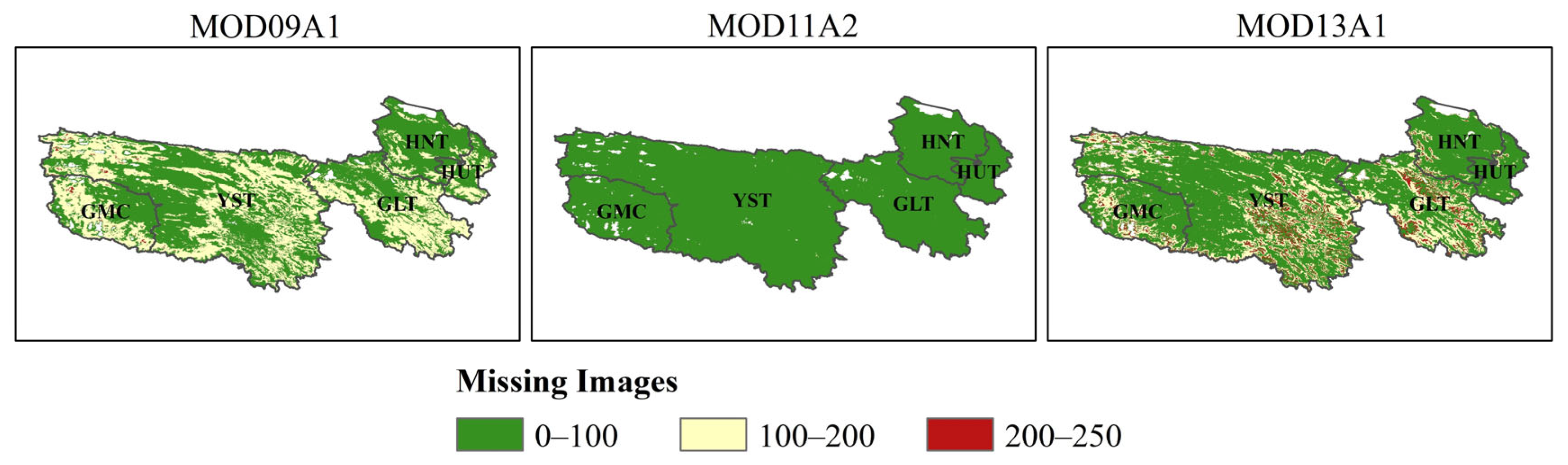
Table 3. Comparison of the proportion of missing pixels before and after processing for abnormal pixel detection.
DataMOD09A1MOD11A2MOD13A1
before the processing27.72%27.72%55.43%
after the processing32.89%29.87%62.65%
Table 4. Four indicator loadings and first principal component contributions from 2001 to 2020.
200120102020
PC1PC2PC3PC4PC1PC2PC3PC4PC1PC2PC3PC4
WET0.1350.6640.3590.6420.3450.4340.2700.7870.0590.6950.3510.624
KNDVI0.9650.216−0.1350.0550.7950.559−0.2080.1120.9870.052−0.1160.100
NDBSI−0.044−0.572−0.2940.765−0.305−0.668−0.3040.607−0.080−0.567−0.2680.775
LST−0.218−0.4310.8760.002−0.395−0.2300.890−0.006−0.127−0.4390.8890.000
Percent eigenvalue/%60.5434.154.710.6062.9031.475.120.5165.3029.045.070.59
Table 5. The area and proportion of RSEI by grade from 2001 to 2020.
RSEI Level20012005201020152020
Area
/103 km2
Pct.
(%)
Area
/103 km2
Pct.
(%)
Area
/103 km2
Pct.
(%)
Area
/103 km2
Pct.
(%)
Area
/103 km2
Pct.
(%)
Very Poor8.12.2310.52.862.20.603.30.892.50.69
Poor49.213.4377.421.1529.37.9947.412.9422.96.27
Moderate106.729.15173.147.28177.848.58185.050.53121.033.05
Good160.643.8798.126.80139.738.16114.031.14138.637.88
Very Good41.411.327.01.9217.04.6616.54.5081.022.12
Table 6. Spatial distribution of RSEI trend from 2001 to 2020.
Theil–Sen Slope/%Z ValueTrend of RSEIPercentage of Area (%)
>0.05>1.96Significant improvement62.96
>0.05−1.96~1.96Slight improvement2.29
−0.05~0.05−1.96~1.96Basically stable23.37
<−0.05−1.96~1.96Slight degradation5.07
<−0.05<−1.96Significant degradation6.32
Table 7. Spatial distribution of RSEI future change trend.
Theil–Sen Slope/%HIFuture TrendsPercentage of Area (%)
−0.050~0.5Reduction–increase trend10.34
0.050.5~1Continuously increasing status33.74
−0.05~0.050.5~1Continuously stable18.14
0.050~0.5Increase–reduction trend21.21
−0.050.5~1Continuously reducing status1.05
−0.05~0.050~0.5Unpredictable change15.52
Table 8. Comparison of the three interpolation methods at different missing ratios. The abbreviations in the table are as follows: Singular Spectrum Analysis (SSA), linear interpolation (LI), cubic spline interpolation (CSI), standard deviation (STD), coefficient of determination (R2), Mean Absolute Error (MAE), and Root Mean Square Error (RMSE).
Set the Missing Ratio to 0.1
Interpolation MethodR2MAERMSE
MeanSTDMeanSTDMeanSTD
SSA0.920.0224.222.541095.10222.21
LI0.840.0247.324.102059.61324.72
CSP0.870.0330.083.251549.79315.83
Set the Missing Ratio to 0.2
Interpolation MethodR2MAERMSE
MeanSTDMeanSTDMeanSTD
SSA0.840.0346.844.261593.60316.84
LI0.760.0352.325.102556.67324.72
CSP0.740.0460.715.383704.06590.24
Set the Missing Ratio to 0.3
Interpolation MethodR2MAERMSE
MeanSTDMeanSTDMeanSTD
SSA0.750.0468.116.742401.60406.16
LI0.640.0672.637.162715.65570.53
CSP0.590.0886.558.904662.25867.68
Set the missing Ratio to 0.4
Interpolation MethodR2MAERMSE
MeanSTDMeanSTDMeanSTD
SSA0.670.0587.9610.442899.03626.44
LI0.560.0896.9811.983458.78697.95
CSP0.470.11110.7112.845058.14898.10
Set the Missing Ratio to 0.5
Interpolation MethodR2MAERMSE
MeanSTDMeanSTDMeanSTD
SSA0.620.07101.5412.333042.14668.41
LI0.490.11127.7317.464220.35709.05
CSP0.310.16138.1619.275689.46925.43
Disclaimer/Publisher’s Note: The statements, opinions and data contained in all publications are solely those of the individual author(s) and contributor(s) and not of MDPI and/or the editor(s). MDPI and/or the editor(s) disclaim responsibility for any injury to people or property resulting from any ideas, methods, instructions or products referred to in the content.

