A Study on the Differences in Vegetation Phenological Characteristics and Their Effects on Water–Carbon Coupling in the Huang-Huai-Hai and Yangtze River Basins, China

Abstract

Vegetation phenology is a biological factor that directly or indirectly affects the dynamic equilibrium between water and carbon fluxes in ecosystems. Quantitative evaluations of the regulatory mechanisms of vegetation phenology on water–carbon coupling are of great significance for carbon neutrality and sustainable development. In this study, the interannual variation and partial correlation between vegetation phenology (the start of growing season (SOS), the end of growing season (EOS), and the length of growing season (LOS)) and ET (evapotranspiration), GPP (gross primary productivity), WUE (water use efficiency; water–carbon coupling index) in the Huang-Huai-Hai and Yangtze River Basins in China from 2001 to 2019 were systematically quantified. The response patterns of spring (autumn) and growing season WUE to SOS, EOS, and LOS, as well as the interpretation rate of interannual changes, were evaluated. Further analysis was conducted on the differences in vegetation phenology in response to WUE across different river basins. The results showed that during the vegetation growth season, ET and GPP were greatly influenced by phenology. Due to the different increases in ET and GPP caused by extending LOS, WUE showed differences in different basins. For example, an extended LOS in the Huang-Huai-Hai basins reduced WUE, while in the Yangtze River Basin, it increased WUE. After extending the growing season for 1 day, ET and GPP increased by 3.01–4.79 mm and 4.22–6.07 gC/m², respectively, while WUE decreased by 0.002–0.008 gC/kgH₂O. Further analysis of WUE response patterns indicates that compared to ET, early SOS (longer LOS) in the Yellow River and Hai River basins led to a greater increase in vegetation GPP, therefore weakening WUE. This suggests that phenological changes may increase ineffective water use in arid, semi-arid, and semi-humid areas and may further exacerbate drought. For the humid areas dominated by the Yangtze River Basin, changes in phenology improved local water use efficiency.

1. Introduction

Vegetation phenology refers to the regular growth and changes in vegetation over an annual cycle after long-term adaptation to the natural geographical environment [1,2]. A large number of studies based on ground observations and remote-sensing monitoring have shown that in the past 30 years, the start of the growing season (SOS) has advanced, and the end of the growing season (EOS) has been delayed in the middle and high latitudes of the Northern Hemisphere [3,4]. Consequently, the length of the growing season (LOS) has increased, but the trend of earlier greening in the past 20 years has slowed down [5]. For example, Piao et al. [6] showed that the change rates of SOS, EOS, and LOS of temperate vegetation in China from 1982 to 2009 were −0.79, 0.37, and 1.16 days/year, respectively. However, owing to the uncertainty of phenological extraction methods, the results are not completely consistent. For instance, there are four perspectives on the phenological fluctuations in the high–cold region of the Qinghai–Tibet Plateau: delayed greening, early greening, no obvious change, and early greening [7]. Recently, many scholars have conducted research on the reasons for this change in phenology in different regions, and climate warming is considered one of the main controlling factors leading to the advancement or delay of phenology [8,9,10]. The early growth of vegetation is influenced by the combined effects of temperature increases in winter and spring, particularly during the daytime [11]. Additionally, vegetation phenology is very sensitive to the effects of precipitation, especially in arid and semi-arid areas. Li et al. [12] indicated that SOS was driven by the beginning of the rainy season in arid and semi-arid areas of the Qinghai–Tibet Plateau. Moreover, some scholars have proposed that climatic variables cannot fully explain the mechanism of phenological changes and that biological factors of vegetation are also key factors controlling phenological changes and differences [13]. Marchand et al. [14] suggested that tree diameter, tree height, and the previous year’s EOS were key factors affecting SOS. The earlier the age of a leaf, the earlier sufficient cooling is required in winter, and the earlier the SOS of the following year. Taller and more dominant trees will have relatively late greening periods.

Vegetation phenology directly or indirectly regulates the water and carbon flux between the land and atmosphere by changing physiological and structural characteristics such as photosynthetic rates and canopy conductance [15]. It plays a key role in the interactions between different species, nutrients, and community compositions, which in turn profoundly affects the water–carbon, nutrient dynamic balance, and biodiversity patterns of the entire terrestrial ecosystem [16,17,18,19]. Water use efficiency (WUE) is a key indicator for evaluating ecosystem functions [20]. It links the carbon cycle, the photosynthesis and transpiration of vegetation, to the water cycle and is an important parameter for understanding carbon–water coupling in terrestrial ecosystems [21]. Vegetation WUE has shown a changing trend in recent decades [22,23,24]. However, owing to timescale and regional differences, the trend of WUE change is not completely consistent. For example, Liu et al. [25] found that annual WUE declined in southern China from 2000 to 2011 owing to a decrease in net primary productivity (NPP) and an increase in evapotranspiration (ET), whereas annual WUE tended to increase in northern China. Ecosystem WUE is affected by multiple factors, with water conditions being the main driver [26]. In most cases, drought inhibits both ecosystem gross primary productivity (GPP) and ET, leading to WUE uncertainties [27]. Currently, more scholars are focusing on the influence of vegetation biological factors on WUE as changes in vegetation phenology may have an important impact on the water–carbon cycle and WUE. For example, Peichl et al. [28] found large variations in the magnitude of GPP_max in peatlands over space and time, which were related to vegetation species composition and phenology rather than abiotic factors. Collins et al. [29] found that LOS was highly correlated with the GPP of tundra vegetation. In simulation research, Piao et al. [30] found that a 1-day increase in LOS in the permafrost zone can lead to a significant increase in annual GPP in the mid-to-high-latitudes of the Northern Hemisphere, considerably enhancing ecosystem carbon sequestration. However, the regulation of WUE by vegetation phenology is not yet fully understood. Conversely, due to the simultaneous control of changes in WUE by ET and GPP and the difference in phenological sensitivity between ET and GPP, the regulatory mechanism of phenology on WUE is more complex. However, the response of WUE to vegetation phenology remains poorly understood in different regions.

The Huang-Huai-Hai and Yangtze River Basins account for approximately 33% of China’s total land area. The geographical heterogeneity of this region is obvious, and the climatic conditions are complex, causing regional land vegetation types to have obvious spatial heterogeneity. At present, research on the impact of changes in vegetation phenology on the interannual changes in GPP, ET, and WUE mainly focuses on a specific vegetation type or climate-sensitive area. For example, Guo et al. [31] studied the impact of vegetation phenology on WUE in typical subtropical ecosystems in Zhejiang Province, China. Zhang et al. [32] explored the potential relationship between phenology and WUE in the Luan River Basin of semi-arid China. Cheng et al. [33] analyzed the relationship between vegetation phenology on the Qinghai–Tibet Plateau and WUE. Although there have been some studies on the impact of vegetation phenology on water use efficiency in the Northern Hemisphere, larger spatial scales may overlook regional differences and fail to clarify the different responses of vegetation water use efficiency to vegetation phenology in humid, semi-humid, and semi-arid regions. Therefore, it is necessary to study the different impacts of vegetation phenology on WUE in the watersheds of China’s major climate zones, which is of great significance for implementing ecological protection measures tailored to local conditions to cope with climate change.

Therefore, the objectives of this study were to (1) evaluate the interannual changes in vegetation phenology, ET, GPP, and WUE in the study area; (2) investigate the response patterns of WUE to phenology in different regions and vegetation types in spring, autumn, and the growing season; and (3) quantify the explanatory power of phenological factors on the interannual variation of WUE, GPP, and ET in different basins.

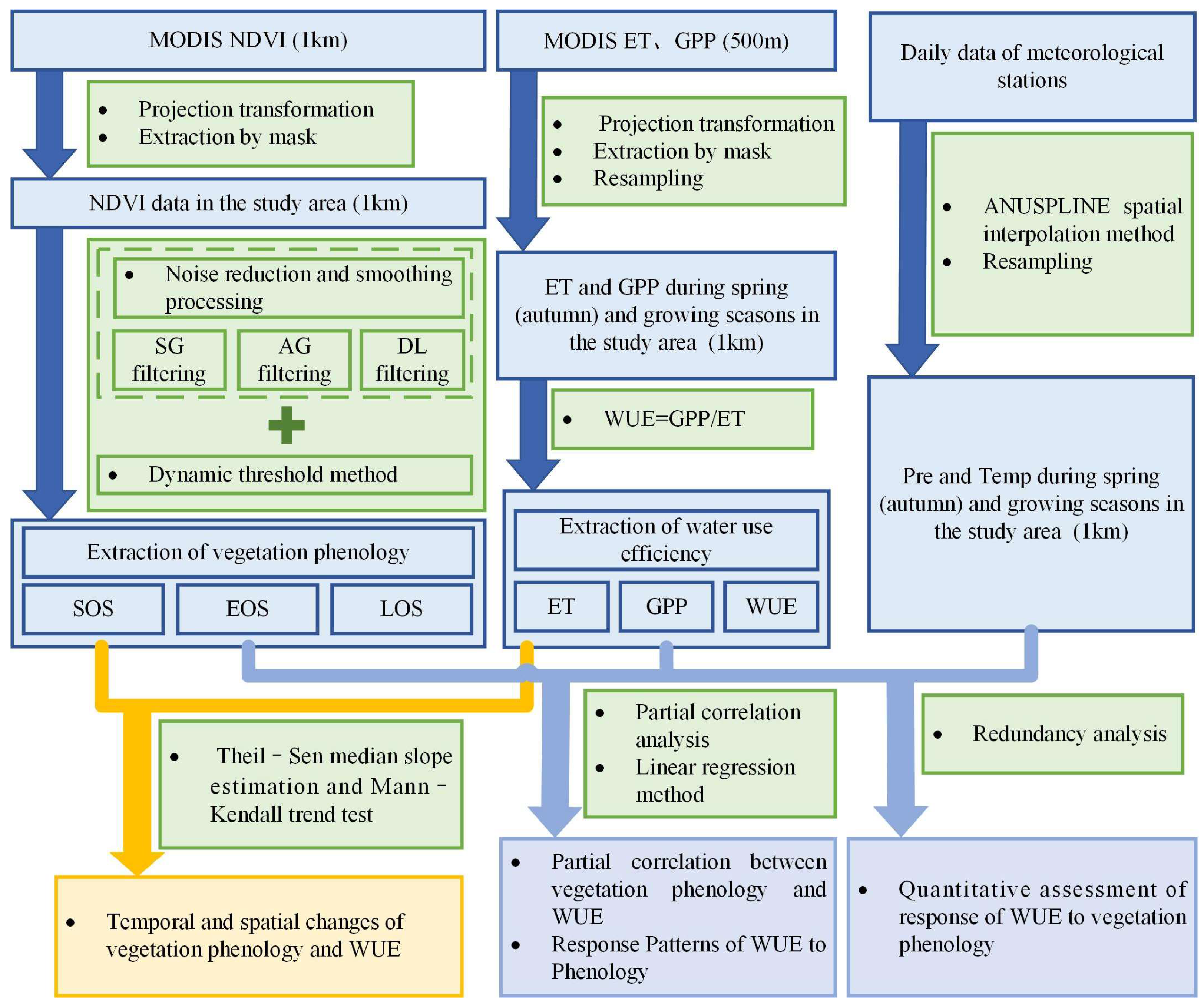
2. Materials and Methods

2.1. Study Area

The study area consists of the Yellow River Basin (YLR), Haihe River Basin (HAR), Huaihe River Basin (HUR) and Yangtze River Basin (YZR), located at 90°32′–122°40′ E and 24°27′–42°43′ N. It covers 21 provinces, cities, and autonomous regions, with a total area of 318.56 × 10⁴ km². The main climate types in this region are temperate and subtropical monsoon climates, temperate continental and plateau mountain climates. Owing to their vast territory, complex terrain, and diverse climatic conditions, different basins have formed unique vegetation types. The northwestern region is dominated by grassland, and the southern region is dominated by forests. As a typical alluvial plain, the northeastern region is a representatively developed agricultural region where wheat and corn are mainly planted. The location of the study area is shown in Figure 1, and a basic overview of the four river basins is presented in

Table 1. Basic overview of the study area.

Basin	Range	Area/ 104 km2	Ta/°C	Pre/mm	Proportion of Vegetation Types/%			Climate Zoning
					Forest	Grassland	Croplands
YZR	24°27′–35°44, 90°32′–121°54′	180	13.3	1100	60.09	18.44	16.70	Humid areas
HAR	35°03′–42°43′, 111°57′–119°44′	32.06	8.8	530	14.07	29.17	48.34	Semi-humid and semi-arid areas
HUR	30°57′–37°49′, 111°56′–122°40′	27	14.1	920	7.79	2.37	79.77	Humid areas
YLR	32°09′–41°49′, 95°54′–119°12′	79.5	9.4	480	9.57	65.54	20.57	Arid and semi-arid areas

.

2.2. Data

Here, the NDVI dataset—sourced from the MODIS vegetation index dynamic product (MOD13A2) provided by National Aeronautics and NASA—was used to extract vegetation phenology. These NDVI products have a spatial resolution of 1 km, a 16-day temporal resolution, and a time span of 2001 to 2019 (https://ladsweb.modaps.eosdis.nasa.gov/, accessed on 1 August 2023). The meteorological data included daily average temperature and daily precipitation from 2001 to 2019, sourced from the daily value dataset of the China Meteorological Data Network (http://data.cma.cn, accessed on 2 August 2023). Monthly meteorological data were obtained using MATLAB R2020a for 417 stations in the study area. ANUSPLINE was then used for interpolation with a spatial resolution of 1 km to match the remote-sensing NDVI data [34,35]. The effects of longitude, latitude, and altitude on various climatic factors were mainly considered in the interpolation process, and the altitude data were based on digital elevation model (DEM) data with a 30 m spatial resolution (http://www.resdc.cn, accessed on 1 August 2023). Gross Primary Production(GPP) and evapotranspiration(ET) datasets were derived from the MODIS Dynamic products (MOD16A2 and MOD17A2) provided by NASA (https://ladsweb.modaps.eosdis.nasa.gov/, accessed on 1 August 2023). The data had a spatial resolution of 500 m and an 8-day temporal resolution. These data were converted to monthly data using ArcGIS and resampled to 1 km [36]. The WUE data were calculated from the GPP and ET datasets. The Land Cover Type dataset was also from MODIS MCD12Q1, with a spatial resolution of 500 m and a 1-year temporal resolution. Since the spatial resolution of different data is different, to facilitate analysis, the resampling tool (nearest interpolation method) in ArcGIS software was used to unify the resolution of the data to 1 km.

2.3. Research Method

The overall research framework is shown in Figure 2. The first step is data processing. MODIS NDVI data were projected and masked to obtain the 1 km NDVI data for the study area. Then, vegetation phenology in the study area (SOS, EOS, and LOS) was extracted using denoising and smoothing techniques, as well as dynamic thresholding methods. MODIS ET and GPP were also used to obtain the GPP and ET of spring (autumn) and the growing season in the study area via projection conversion, mask extraction, and resampling (nearest interpolation method). WUE data were obtained by dividing GPP and ET. ANUSPLINE and time resampling were used to convert daily meteorological station data into 1 km meteorological raster data (precipitation and temperature) for spring (autumn) and the growing season in the study area. Then, the Theil–Sen median slope estimation and Mann–Kendall trend test were used to analyze the spatio-temporal evolution of vegetation phenology and WUE. Partial correlation analysis and the linear regression method were used to evaluate the correlation between vegetation phenology and WUE in spring (autumn) and the growing season and further revealed the response model of WUE to phenology. In addition, the effects of climate and phenological factors on ET, GPP, and WUE were quantitatively evaluated via redundancy analysis.

2.3.1. Calculation of Water Use Efficiency

The water use efficiency was calculated from evapotranspiration and total primary productivity. The calculation formula is as follows:

$$WUE={\displaystyle \frac{GPP}{ET}}$$

(1)

where WUE (gC/kgH₂O) is the annual water use efficiency. GPP (gC/km²) is the annual gross primary productivity, and ET (mm) is the annual evapotranspiration.

2.3.2. Determining the Phenology

Before extracting the phenological indicators, the NDVI data must be preprocessed. Because cultivated land, wetlands, deserts, urban land, water bodies, and the interaction area between farmland and vegetation have been seriously disturbed by human activities, and the vegetation is unstable, these pixels should be eliminated. NDVI data corresponding to the remaining vegetation cover types were used as input data for phenological extraction.

(1)

Noise reduction and smoothing processing

Due to the significant influence of clouds and atmosphere on remote-sensing image acquisition, it is necessary to denoise and smooth NDVI time series. This can remove outliers and local mutation points in NDVI data without being limited by the time and spatial scale of the data and sensors [37]. To improve accuracy, three smoothing methods were selected to fit NDVI separately, including the asymmetric Gaussian function fitting method, the double logistic function fitting method, and the Savitzky–Golay filtering method.

(a)

Savitzky–Golay filtering method (SG)

The method was proposed by Savitzky and Golay in 1964 [38]. Based on the local polynomial regression model, the least squares method was used to best fit the data within the filter window. The formula used is as follows:

$$Y_j={\displaystyle \frac{{\displaystyle \sum _{i=-n}^{i=n}{C}_i{Y}_{j+1}}}{N}}$$

(2)

where Y_j+1 represents the original data, Y_j represents the fitting value, C_i represents the weight of the ith point, and N = 2n + 1 represents the size of the filter window. After reference and repeated testing, the window value was set to three.

(b)

Asymmetric Gaussian function fitting method (AG)

Proposed by Jonsson and Eklundh in 2002, this fitting method builds a local fit into a whole [39,40]. The vegetation growth process was simulated using a Gaussian function based on the valley and peak values, and the local fitting functions were integrated based on the global fitting function. The local fitting function is expressed as follows:

$$f(t)=f(t;c_1,c_2,a_1,a_2,\cdots ,a_5)=c_1+c_{2}g(t;a_1,\cdots ,a_5)$$

(3)

$$g(t;a_1,\cdots ,a_5)=\{\begin{array}{l}\exp \left[-{\left({\displaystyle \frac{t-a_1}{a_2}}\right)}^{a_3}\right],t>a_1\\ \exp \left[-{\left({\displaystyle \frac{a_1-t}{a_4}}\right)}^{a_5}\right],a_1<t\end{array}$$

(4)

where g(t, a₁, a₂, ..., a₅) represents the Gaussian function; c₁ and c₂ represent the reference and amplitude of the control curve, respectively; a₁ determines the position of the peak and valley values; and a₄, a₅, a₂, and a₃ control the width and steepness of the left and right sections of the curve, respectively.

(c)

Double logistic function fitting method (DL)

This method—proposed by Beck in 2006 [41]—is based on a local fitting function (double logistic function) to construct an overall function as follows:

$$g(t;a_1,\cdots ,a_4)={\displaystyle \frac{1}{1+\exp \left(\frac{a_1-t}{a_2}\right)}}-{\displaystyle \frac{1}{1+\exp \left(\frac{a_3-t}{a_4}\right)}}$$

(5)

where g(t, a₁, ..., a₄) represents a double logistic function, and a₁, a₂, a₃, and a₄ control the inflection point position and change rate at the inflection points on the left and right parts of the curve, respectively. The overall fitting function is the same as that of the AG fitting function.

(2)

Phenological extract

Currently, commonly used methods for extracting phenology include the dynamic threshold method [42], the extreme value method of curvature change [43], the moving average method [44], and the maximum rate of change method [3]. Here, the dynamic threshold method was used to obtain the SOS, EOS, and LOS for each pixel at the pixel scale. Because different scholars have set different thresholds according to different study areas in the process of phenology extraction, the dynamic thresholds of SOS and EOS were set to 20% and 80%, respectively, based on repeated trials.

2.3.3. Analysis Methods

(1)

Trend analysis

Here, Theil–Sen median slope estimation and Mann–Kendall trend test were used to determine the trend and significance in vegetation phenology, ET, GPP, and WUE. Theil–Sen median slope estimation is a trend calculation method for nonparametric statistics. This method is suitable for trend analysis of long time-series data [45]. The formula is as follows:

$$\beta =Median\left({\displaystyle \frac{x_j-x_i}{j-i}}\right),\forall j>i$$

(6)

where β represents Sen’s slope; the Median () is the median function; when β < 0, it exhibits a decreasing trend, and when β > 0, an increasing trend is observed.

The Mann–Kendall trend test method was mainly used to judge the mutation points of the time series and determine the significance of the phenological series to analyze the phenological trend [46].

(2)

Partial correlation analysis

Because the simple correlation does not take into account the multiple collinearities between vegetation and climate variables, the effects of vegetation phenology on ET, GPP, and WUE cannot be accurately assessed. Therefore, a high-order partial correlation analysis method was adopted, with precipitation and temperature as control variables, to evaluate the correlation between vegetation phenology and ET, GPP, and WUE in different seasons. Assuming there are k (k ≥ 2) variables x₁, x₂, ... x_k, the formula for calculating the n (n ≤ k − 2) order partial correlation coefficients of any two variables x_i and x_j are as follows:

$$r_{ij·l_1{l}_2\cdots l_n}={\displaystyle \frac{r_{ij·l_1{l}_2\cdots l_{n-1}}-r_{i{l}_n·l_1{l}_2\cdots l_{n-1}}{r}_{j{l}_n·l_1{l}_2\cdots l_{n-1}}}{\left(1-r_{i{l}_n·l_1{l}_2\cdots l_{n-1}}^2\right)\left(1-r_{j{l}_n·l_1{l}_2\cdots l_{n-1}}^2\right)}}$$

(7)

where r_ij represents the partial correlation coefficient between i (phenology) and j (WUE), and the control variables are temperature and precipitation. The value of the partial correlation coefficient ranges from −1 to 1. The closer the absolute value of the correlation coefficient is to 1, the better the correlation.

(3)

Linear regression analysis

To determine the sensitivity of ET, GPP, and WUE to vegetation phenology in spring (autumn) and the growing season, a univariate linear regression analysis was carried out with phenology as independent variables and ET, GPP, and WUE as dependent variables (regression slope represents the sensitivity of WUE to phenology). The calculation formula is as follows:

$$G={\displaystyle \frac{n\times {\displaystyle \sum _{i=1}^n\left(i-P_i\right)-{\displaystyle \sum _{i=1}^{n}i{\displaystyle \sum _{i=1}^n{P}_i}}}}{n\times {\displaystyle \sum _{i=1}^n{i}^2}-{\left({\displaystyle \sum _{i=1}^{n}i}\right)}^2}}$$

(8)

where G represents the regression slope, n represents the number of samples, i represents the phenology, and P_i represents the water use efficiency index corresponding to the phenological period.

(4)

Redundancy analysis

Redundancy analysis is a ranking method that combines multi-response variable regression analysis and principal component analysis [47]. This clearly explains the relationship between the response and explanatory variable matrices. Redundancy analysis was used to evaluate the contributions of temperature, precipitation, and phenology to WUE, and Monte Carlo analysis was used to analyze factor significance.

3. Results

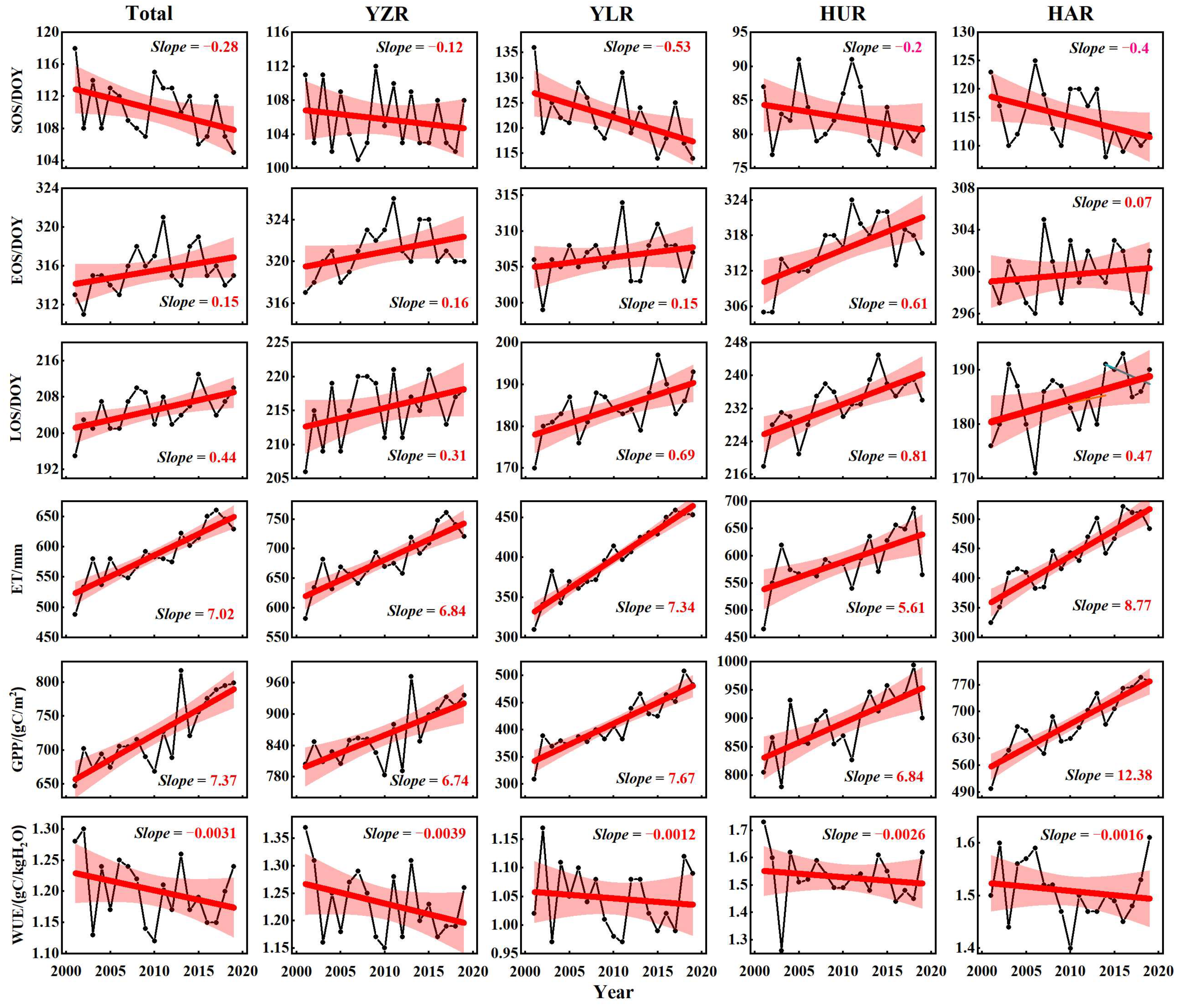
3.1. Temporal Variation of the Vegetation Phenology and WUE

Figure 3 and Figure 4 illustrate the interannual changes and spatial distributions of vegetation phenology, ET, GPP, and WUE in the study area from 2001 to 2019. Figure 5 shows the proportion of changes in the above variables in each basin. The SOS in the study area showed an early trend, with an overall annual advance of 0.28 days. There were differences in SOS among different basins, and the advance rate was ranked as YLR (0.53 days/year), HAR (0.40 days/year), HUR (0.2 days/year), and YZR (0.12 days/year) in descending order. In total, 71.7% of the regions in the study area showed an early trend in terms of SOS, with significant and extremely significant early trends accounting for 13.8%. From different basins, the proportion of regions with an early trend in terms of SOS in the HAR (85.5%) and the YLR (78.4%) was relatively high, with significant and extremely significant early trends accounting for 12.3% and 20.5%, respectively. Meanwhile, 61.6% and 61.4% of the vegetation in the HUR and the YZR showed an advance trend in SOS, with significant and extremely significant advance trends accounting for 13.5% and 8.9%, respectively. Similarly, the EOS generally exhibited a late trend with a rate of 0.15 days/year. The trend of EOS in the HUR was the largest (0.61 days/year), followed by the YZR (0.16 days/year), YLR (0.15 days/year), and HAR (0.07 days/year). In total, 64.7% of the regions in the study area showed a late trend in EOS, with a significant and extremely significant proportion of 9.2%. From different river basins, HUR had the highest proportion of regions with a late trend in EOS (82.9%), with significant and extremely significant late trends accounting for 34.5%, respectively. Next were the YZR (60.7%), YLR (60%), and HAR (55.2%), with significant and extremely significant late trends accounting for 9.1%, 9.4%, and 3.7%, respectively. LOS was jointly determined by SOS and EOS. Owing to the advancement of SOS and the delay in EOS, the entire study period showed a trend of extension (0.44 days/year). Among all basins, HUR had the largest LOS extension (0.81 days/year), followed by YLR (0.69 days/year), HAR (0.47 days/year), and YZR (0.31 days/year). In total, 75.9% of the regions in the study area had an extended LOS trend, with approximately 18% of the regions showing significant and extremely significant extension trends. From different river basins, the proportion of vegetation LOS in the HAR showing an extended trend was the highest (78.6%), followed by the HUR (77.9%), the YLR (74%), and the YZR (73.1%). Overall, the SOS changes in the YLR (arid and semi-arid areas) and the HAR (semi-arid and semi-humid areas) are more significant, while the vegetation EOS changes in YZR and HUR (humid areas) are more pronounced.

The increase rate of ET in the whole study area was 7.02 mm/year, with the fastest increase rate in the HAR (8.77 mm/year) and the slowest in the HUR (5.61 mm/year). An increasing trend in ET was observed in 92.8% of the regions, of which 75.1% showed a significant or extremely significant increase. From different river basins, over 95% of the regions in the HAR, YLR, and YZR showed an increasing trend in terms of ET, with 94.7%, 91.8%, and 62.2% showing significant and extremely significant increasing trends, respectively. Only 77.5% of the regions in the HUR showed an increasing trend in terms of ET, with a significant and extremely significant increase in the area accounting for 51.9%. The GPP increase rate was 7.37 gC/(m²·year), with 90.7% of the regions showing an increasing trend. From different river basins, both the HAR and the YLR had an increasing trend of ET in over 96% of the regions, with the proportion of areas showing significant and extremely significant increases of 92.7% and 69.8%, respectively. In total, 88.8% and 79.5% of the regions in the YZR and HUR showed an increasing trend in terms of ET, with 39.5% and 56.3% of the areas showing significant and extremely significant increasing trends, respectively. WUE showed a slight decreasing trend during the study period, with an overall decrease rate of 0.0031 gC/(kgH₂O·year). The YZR decreased the fastest (0.0039 gC/(kgH₂O·year)), followed by HUR (0.0026 gC/(kgH₂O·year)), HAR (0.0016 gC/(kgH₂O·year)), and YLR (0.0012 gC/(kgH₂O·year)). WUE showed a significant increasing trend in the central and western parts of the YLR as well as in the southwestern part of the YZR. In the study area, 61.9% of the regions showed a decreasing trend in terms of WUE, and 10.2% of the regions showed significant and extremely significant decreasing trends. In terms of river basins, the proportion of WUE decreasing in the YZR was the largest (67.4%), followed by HUR (61.5%), HAR (60.7%), and YLR (58%). Overall, the vegetation ET and GPP in the YLR (arid and semi-arid areas) and the HAR (semi-arid and semi-humid areas) grew faster, while vegetation WUE in the YZR and HUR (humid areas) decreased more.

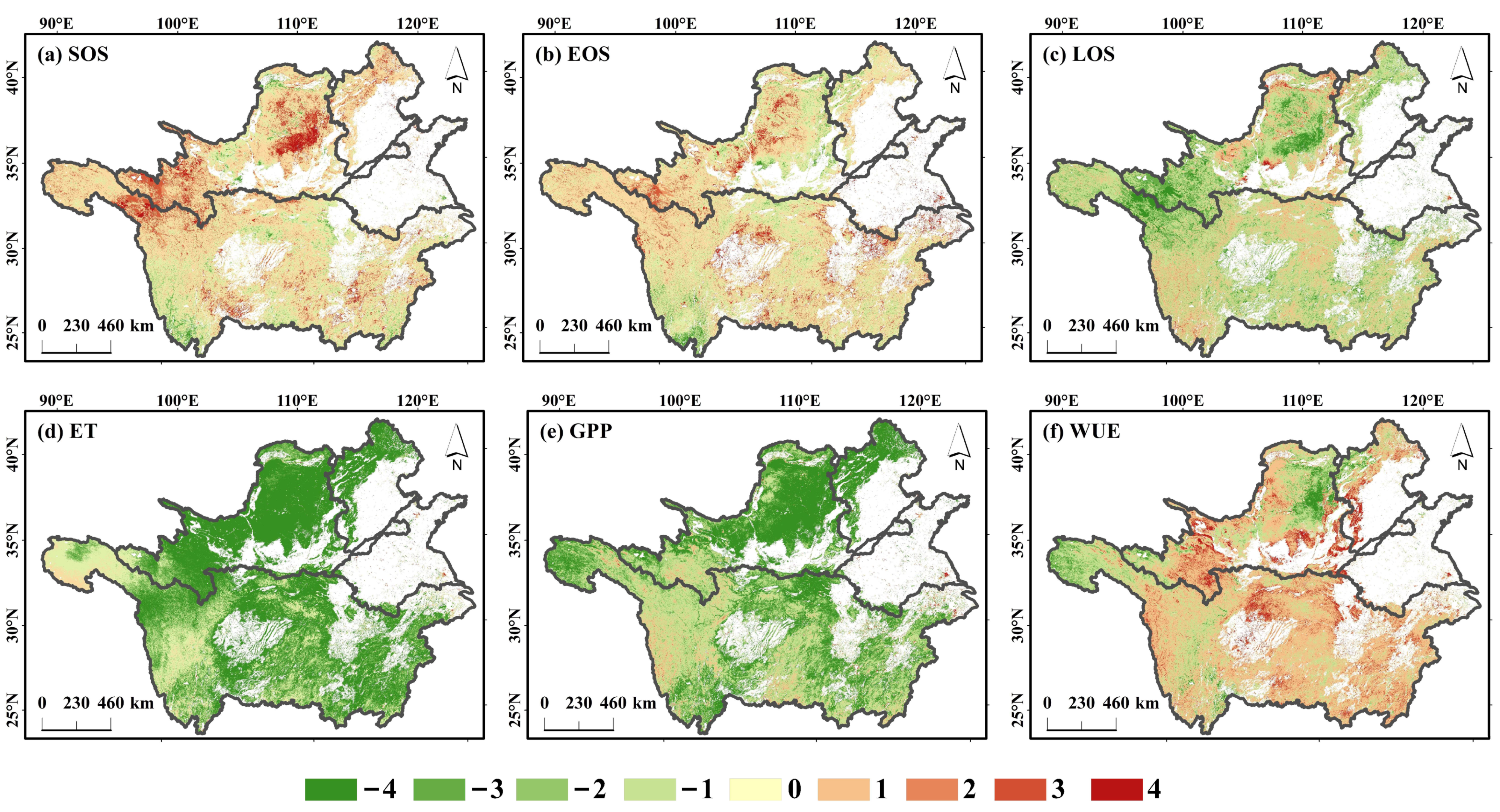
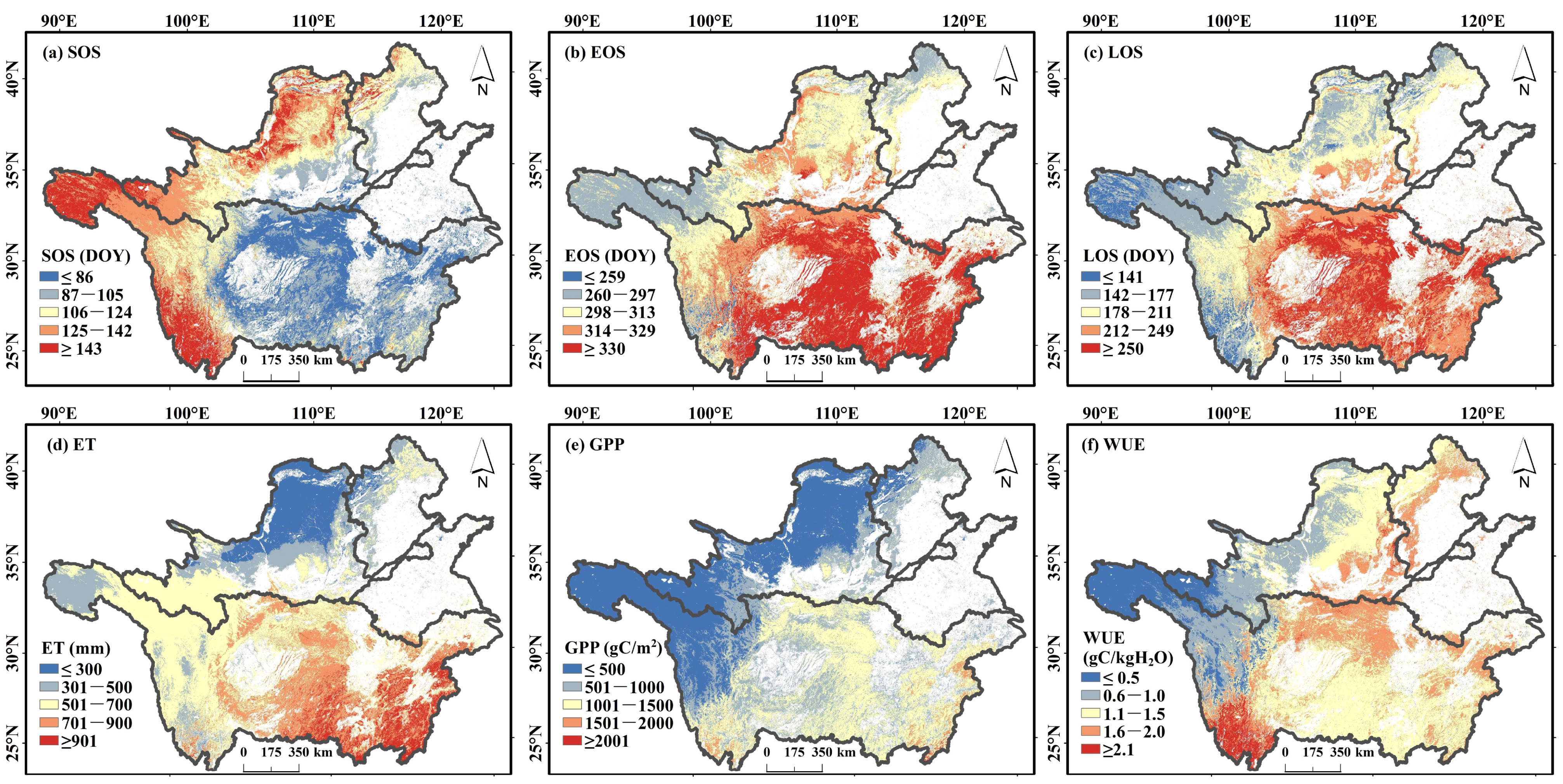
3.2. Spatial Distribution of the Vegetation Phenology and WUE

The annual average spatial distributions of vegetation phenology, ET, GPP, and WUE in the study area are shown in Figure 6. The average annual SOS in the study area occurred on the 110th day, and approximately 94.5% of the vegetation SOS occurred from early March to late May. The average annual SOS rankings for each basin were as follows: YLR (the 122nd day) > HAR (the 115th day) > YZR (the 106th day) > HUR (the 83rd day). The SOS in the western and northern regions of the YLR occurred later, whereas those in the middle and lower reaches occurred earlier. The SOS occurred late in the deep mountainous area north of the HAR and early in the shallow mountainous area. The HUR was in a plain area with suitable temperature and precipitation, and its SOS was earlier than that of other river basins. In the upper reaches of the YZR, the SOS was late, and the middle and lower reaches were earlier. The multi-year average EOS occurred on the 316th day, with approximately 88.8% of the vegetation EOS occurring from early September to early December in the 240–340 days range. The annual average EOS ranking of the basin was YZR (the 321st day) > HUR (the 316th day) > YLR (the 306th day) > HAR (the 300th day). The EOS spatial distribution was opposite to that of SOS and gradually decreased from south to north. The average annual LOS was 205 days, and approximately 97.1% of the LOS was in the range of 130–270 days (3–11 months). The LOS was shorter in the western and northern regions and longer in the southern regions. Overall, these results are consistent with those of previous studies conducted in the study area (

Table A1. A comparison of estimated dates for phenological events derived from this study and previously published data.

Study Area	Methods	Study Period	SOS (DOY)	EOS (DOY)	LOS (DOY)	Data Resources	Article
Loess Plateau (Mainly located in the YLR)	SG	200–2018	96–144	288–304	–	MODIS MOD13Q1	Pei et al. [37]
YLR	SG	2001–2020	90–160	270–310	110–190	MODIS MOD13Q1	Wang et al. [70]
YLR	DL	2001–2020	80–160	270–300	150–200	GOSIF dataset	Wang et al. [71]
Jing-jin-ji (Mainly located in the HAR)	SG	2001–2020	99 (forest), 102 (grassland)	287 (forest), 279 (grassland)	188 (forest), 178 (grassland)	MODIS MOD13Q1	Zhang [72]
Jing-jin-ji (Mainly located in the HAR)	–	2000–2018	92–149 (forest), 90–132 (grassland)	213–299 (forest), 236–300 (grassland)	–	Actual station phenological data	Zhang [72]
YZR	SG	1982–2015	70–160	220–312	130–230	GIMMS NDVI3g	Yuan et al. [73]
YLR, YZR, HAR, HUR	SG, DL, and AG	200–2019	106 (YZR), 83 (HUR), 122 (YLR), 115 (HAR)	321 (YZR), 316 (HUR), 306 (YLR), 300 (HAR)	215 (YZR), 233 (HUR), 184 (YLR), 185 (HAR)	MODIS MOD13A2	Our study

Notes: DOY, day of the year, i.e., Julian Day. YLR, Yellow River Basin. YZR, Yangtze River Basin. HAR, Haihe River Basin. HUR, Huaihe River Basin. SG, Savitzky—Golay filtering method. AG, Asymmetric Gaussian function fitting method. DL, Double Logistic function fitting method.

). Vegetation in arid and semi-arid regions and semi-humid regions has a later SOS and an earlier EOS, resulting in a shorter growth season compared to vegetation in humid regions.

The average annual ET in the study area was 586.4 mm, with the highest ET in the southeast, followed by the southwest, and the lowest in the arid region of the northwest, owing to water conditions. The annual average GPP was 723.5 gC/m², and the spatial GPP was higher in the southeastern coastal area but lower in the Qinghai–Tibet Plateau, Loess Plateau, and Haihe Mountain region. The annual average WUE was 1.2 gC/kgH₂O, with HUR having the highest annual average WUE of 1.53 gC/kgH₂O, followed by the HAR (1.51 gC/kgH₂O), YZR (1.20 gC/kgH₂O), and YLR (1.04 gC/kgH₂O). This is basically consistent with some previous research results (

Table A2. A comparison of estimated dates for WUE, derived from this study and previously published data.

Study Area	Study Period	Annual Average WUE (gC/kgH2O)	Data Resources	Article
Yellow River Basin	2001–2020	1.55	MODIS MOD17A2(GPP) MOD16A2(ET)	Chen [74]
Yellow River Basin	1982–2018	0.51–1.44	GLASS	Liu et al. [75]
Haihe River basin	2000–2014	1.52	MODIS MOD17A2(GPP) MOD16A2(ET)	Zhao et al. [76]
Huaihe River basin	1995–2004	0.83–1.52	Vegetation Integrative Simulator for Trace Gases	Ito and Inatomi [77]
Huaihe River basin	2003–2012	1.54–1.72	MODIS MOD17A3(GPP) MOD16A3(ET)	Qiu et al. [78]
China	2001–2021	0.78–1.43	MODIS MOD17A2(GPP) MOD16A2(ET)	Li et al. [79]
China	2003–2010	0.37–3.1	Flux data	Xiao et al. [80]
China	2003–2020	1.3–2.7	Flux data	Dou et al. [81]
YLR, YZR, HAR, HUR	2001–2019	1.2 (YZR), 1.53 (HUR), 1.04 (YLR), 1.51 (HAR)	MODIS MOD17A2(GPP) MOD16A2(ET)	Our study

Notes: YLR, Yellow River Basin. YZR, Yangtze River Basin. HAR, Haihe River Basin. HUR, Huaihe River Basin.

). Owing to the combined action of ET and GPP, the WUE in the west was lower than that in the east.

3.3. Relationship between Vegetation Phenology and WUE

The partial correlation and regression relationship between vegetation phenology and seasonal ET, GPP, and WUE are shown in Figure 7 and Figure 8. At the pixel scale, vegetation ET and GPP in spring were negatively correlated with SOS, with significantly negatively correlated areas accounting for 20.9 and 30.5%, respectively (Figure 7a,b). These pixels were mainly concentrated in the upper reaches of the YLR, the Loess Plateau of the YLR, hilly areas of the HAR, and central and western areas of the YZR. When SOS advanced by 1 day, spring ET and GPP increased by 0.01–0.02 mm/day and 0.02–0.05 gC/(m²·day) (Figure 8a,b). The relationships between autumn ET, GPP, and EOS were weak (Figure 7d,e). The proportion of positive correlations was slightly higher (56.7 and 66.4%) in the western and central parts of the YZR, western parts of the YLR, and the shallow mountains of the HAR. When EOS was delayed by 1 day, autumn ET and GPP increased by 0.01–0.02 mm/day and 0.001–0.02 gC/(m²·day) (Figure 8d,e). In addition, 69.4 and 70.7% of growing season ET and GPP, respectively, were positively correlated with LOS (Figure 7g,h). With the extension of LOS, the growth season ET and GPP in the western and central regions of the YLR and the northern region of the HAR showed an increasing trend. For each day of LOS extension, ET and GPP increased by 3.01–4.79 mm and 4.22–6.07 gC/m², respectively, during the growth season in the four basins (Figure 8g,h).

The proportion of negative correlations between spring WUE and SOS was relatively high (57.5%) (Figure 7c). When SOS advanced by 1 day, the WUE of the total study area increased by 0.01 gC/kgH₂O (Figure 8c). The relationship between WUE and EOS in autumn is weak (Figure 7f). When EOS was delayed by 1 day, the WUE of the total study area decreased by 0.01 gC/kgH₂O (Figure 8f). The proportion of WUE negatively correlated with LOS during the growing season was 51.2% (Figure 7i) and was mainly distributed in the northern part of the study area, whereas the positively correlated area was mainly distributed in the YZR. When LOS was extended by 1 day, the WUE of the total study area decreased by 0.003 gC/kgH₂O (Figure 8i). Notably, there was no significant spatial correlation between WUE and phenology in spring, autumn, or during the growing season. It indicated that vegetation phenology may not directly cause changes in WUE but may indirectly alter WUE by affecting ET and GPP.

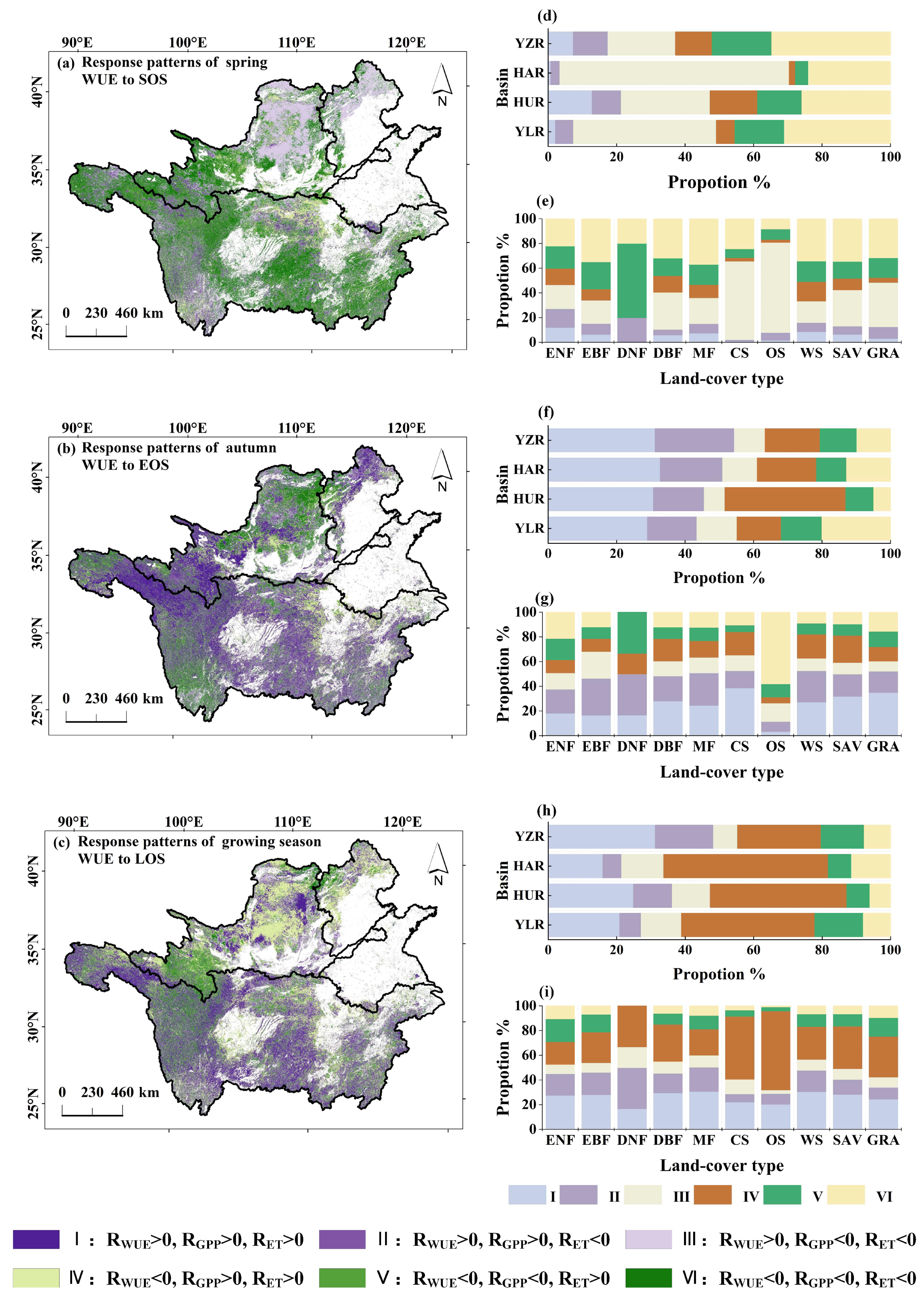
3.4. Response Patterns of WUE to Phenology

Six response modes of WUE to vegetation phenology were divided based on the partial correlation between vegetation phenology and WUE. Figure 9 shows the spatial distribution of WUE response patterns to vegetation phenology and its proportion in the four basins and plant functional types. The results showed that the study area was dominated by modes III and VI in spring. The proportion of Mode III in the HAR and YLR was relatively high, accounting for 66.9% and 41.5% of the effective pixels, respectively. Mode VI had a relatively high proportion in the YZR and HUR, accounting for 34.7% and 25.9% of the effective pixels, respectively. This means that in the northern regions—in which the HAR and YLR are mostly situated—the advance of spring SOS caused vegetation to start photosynthesis and accumulate biomass earlier, and increased leaf area also increased spring ET. The faster increase in ET compared to GPP resulted in a decrease in WUE. In the southern region, WUE increased because GPP increased faster than ET. The response mode of WUE to EOS in autumn differed from that in spring. Modes I, II, and IV mainly occurred in the four basins in autumn, accounting for 30.8%, 17.6%, and 20.3% of the effective pixels, respectively. The positive correlation between autumn GPP and EOS indicated that autumn GPP mainly increased owing to delayed EOS, possibly related to a longer photosynthetic period. However, EOS exhibited significant uncertainty in autumn ET. However, even if ET increased, the intensity of the increase was smaller than that of GPP. During the entire growing season, the four basins were dominated by modes IV and I, accounting for 37.7% and 23.2% of the effective pixels, respectively. YZR was mainly based on Model I, indicating that due to the extension of the growing season, the increase in GPP was stronger, leading to an increase in WUE. However, in other basins, the decrease in WUE caused by the extension of the growing season was more pronounced, mainly due to the increase in ET, which was stronger than the increase in GPP.

From the plant function types, we found that 24.1 and 28.5% of forests (ENF, EBF, DNF, DBF, and MF) were dominated by modes V and VI in spring, respectively. Overall, 67.5 and 16.3% of shrubs (OS and CS) were in modes III and VI, respectively. Grassland (SAV and GRA) was mainly dominated by modes VI and III, accounting for 33.5 and 27.5% of the effective pixels, respectively. This indicated that for more than half of the forests in the study area, their WUE increases with the advancement of SOS. This effect was mainly due to an increase in GPP that was stronger than ET or a decrease in GPP. For shrublands and grasslands, we found that both GPP and ET increased in spring owing to the advancement of the greening period, but the strength of the increase was different, which led to a positive or negative effect of WUE on SOS. For autumn, regardless of the vegetation type, the response pattern was relatively more complex. On the one hand, it may be due to the insignificant increase in autumn phenology, and on the other hand, the changes in GPP, ET, and WUE were less limited by non-phenological factors. Throughout the growing season, the forest and grassland were mainly dominated by modes I, IV, and II, accounting for 26.5%, 25.4%, and 20.8% of the effective pixels, respectively, whereas the shrubs were mainly dominated by modes IV and I, accounting for 57.2% and 21.1% of the effective pixels, respectively. Similar to spring, WUE increased or decreased during the growing season, depending on the relative changes in GPP and ET.

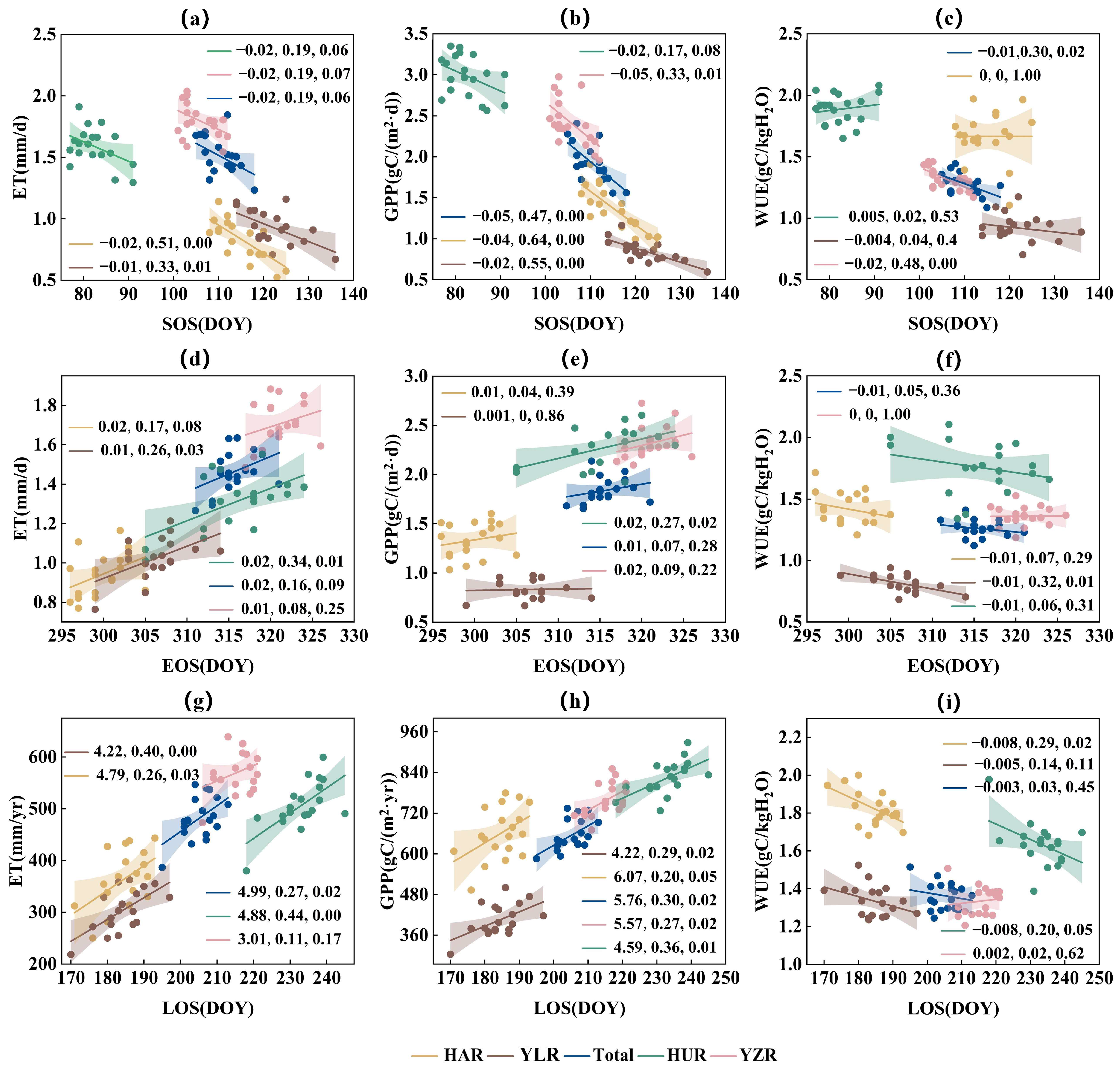
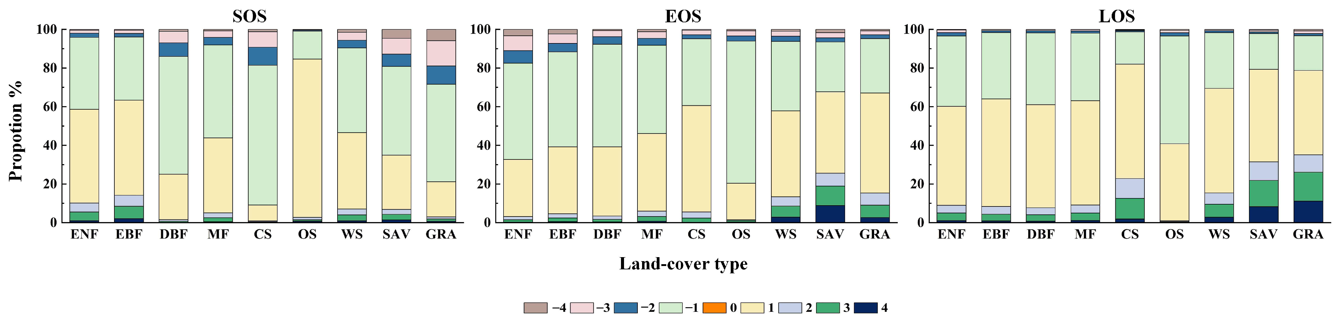
3.5. Quantitative Assessment of Response of WUE to Vegetation Phenology

With the extension of the vegetation growth season and the increase in leaf area during the growth stage, transpiration and photosynthesis of vegetation increase, causing vegetation to transport more water vapor to the atmosphere and fix more carbon. Therefore, vegetation phenology plays an important role in regulating the water and energy balance in terrestrial ecosystems. It can be seen from the previous chapter that vegetation phenology plays an important role in regional, seasonal ET, GPP, and WUE changes. To quantitatively analyze the responses of ET, GPP, and WUE to vegetation phenological indices in the study area, the contribution rates of temperature, precipitation, and phenology to the above three factors were evaluated using redundancy analysis, and the factor significance was analyzed via a Monte Carlo simulation. As shown in Figure 10, for the entire study area, the interannual variation in spring evaporation was significantly affected by SOS, with an explanatory rate of 20.3% (p < 0.05), while evaporation in autumn was significantly affected by precipitation (interpretation rate: 37.6%; p < 0.01). The interannual variation in evaporation during the entire growing season was significantly affected by mean temperature, precipitation, and LOS; however, the explanation rate of temperature was higher than that of precipitation and LOS, at 36.3 (p < 0.01), 23.6 (p < 0.01), and 11.5% (p < 0.05), respectively. Spring GPP was significantly influenced by the average temperature in spring, with an explanatory rate of 44.1% (p < 0.01), while during the growing season, GPP was jointly affected by temperature and LOS with explanatory rates of 35.4 (p < 0.05) and 18.1% (p < 0.05), respectively. WUE was significantly affected by temperature and SOS in spring, with SOS accounting for 7.6% of the changes; however, for autumn and the entire growing season, LOS had a smaller impact on WUE.

The responses of temperature, precipitation, and phenological factors to ET, GPP, and WUE differed significantly between basins. For the HAR, the SOS significantly affected the ET, GPP, and WUE of spring vegetation, with explanatory powers of 51.2, 64.3, and 16.4%, respectively, whereas precipitation may play a more critical role in autumn and the entire growing season. For YLR, because of the semi-arid area, precipitation had a greater impact on different seasons owing to the limitation of water conditions. During the entire growing season of the YLR, precipitation and LOS played key roles in ET, GPP, and WUE, and the explanatory power of LOS was 27.7, 19.1, and 14.4%, respectively. HUR, ET, GPP, and WUE in spring (autumn) were greatly affected by precipitation. For the whole growing season, the effects of the extension of LOS on various elements cannot be ignored. YZR, in typical humid areas, had fewer water constraints, so the temperature during different seasons and growth periods contributed more to ET, GPP, and WUE.

4. Discussion

4.1. Phenological Changes and Spatial Heterogeneity

From 2001 to 2019, a trend of early SOS and late EOS in the four was found in the four major river basins; thus, LOS was prolonged. Environmental factors had significant effects on vegetation phenology [48]. Climate warming has been identified as a major factor in vegetation phenological changes in temperate regions [49]. The SOS and EOS of vegetation are extremely sensitive to temperature changes [50,51,52]. However, a recent study found that a continuous increase in temperature reduces the sensitivity of SOS to temperature [10]. Additionally, the effects of water stress cannot be ignored, as in arid and semi-arid areas, water shortages would inhibit the use of light and heat by local vegetation, resulting in changes in the phenological development of vegetation over time [53,54].

In addition, functional types of vegetation may also be the main factors affecting the spatial heterogeneity of vegetation phenological changes. Our study found that phenological changes in grasslands were more obvious than those in forests, where 72% of grasslands showed an advanced SOS; only 52.2% of forests showed this (Figure 11). Grasslands are relatively fragile ecosystems with shallower root systems than tall trees and are more susceptible to increasing climate change impacts. In the northwestern YLR and western YZR, arid and semi-arid climatic conditions make the grasslands more vulnerable to water stress. Therefore, an increase in spring precipitation stimulates soil water availability, plant photosynthesis, and leaf carbohydrate concentration, which may lead to the advancement of SOS and produce legacy effects [55]. However, the controlling effect of precipitation on the spring phenology of grasslands is weakening, indicating that other potential factors may need further attention [56]. Moreover, in the YZR, where forest vegetation dominates, relatively sufficient water can allow the large roots of trees to buffer water pressure. Therefore, temperature may be the main factor controlling forest vegetation changes [57]. An early rise in temperature in spring may promote forest SOS and prolong the growing season and vegetation growth. However, this effect may weaken as the latitude decreases from high to low [58].

4.2. Response of WUE to Phenology, Temperature and Precipitation

In Section 4.2, we found that the susceptibility of WUE to phenology varied significantly between regions and species and was spatially fragmented, similar to the results of previous studies [59]. The response of WUE to phenology is coupled with the responses of GPP and ET. Furthermore, seasonal changes in phenology regulate vegetation photosynthesis and transpiration, changing GPP and ET and ecosystem material circulation and energy flow [60]. In spring, the advancement of SOS may lead to a larger leaf area and increased light interception, leaf photosynthetic rate, and transpiration rate, therefore increasing GPP and ET [61]. Our study found that the northern basin dominated by the YLR and HAR in spring was dominated by Mode III (ET increase is stronger than GPP), meaning that ineffective water consumption in the northern region may be increased with advancing SOS. In the YZR, the increase in GPP was stronger than that in ET, which improved water use efficiency. In autumn, extended autumn phenology causes leaves to age later, increasing the time for photosynthesis from the leaf to the canopy and increasing GPP [31]. Although EOS prolonged transpiration, there was uncertainty regarding ET because temperature and soil moisture are often low [33]. More average response pattern categories in fall further support this hypothesis.

In Section 4.3, we also found significant differences in the responses of temperature, precipitation, and phenological factors to ET, GPP, and WUE among watersheds. For example, in arid and semi-arid areas (YLR), precipitation has a higher degree of explanation for the changes in ET, GPP, and WUE in spring, autumn, and the entire growing season. In semi-arid and semi-humid areas (HAR), SOS significantly affects ET, GPP, and WUE in spring, while precipitation plays a dominant role throughout the growing season. For vegetation in humid areas (YZR), due to relatively sufficient water, temperature may be more important in terms of affecting the WUE of plants. However, the impact of WUE on climate, phenology, and other factors also varies significantly in other regions of the world. For example, in the desertified areas of northeastern Brazil, seasonal rainfall is a key factor in regulating ecosystem GPP due to significant water constraints [62], while in the tropical rainforest areas of Brazil, water use efficiency is strongly controlled by the number of consecutive drought days, rather than the total precipitation [63]. There are also significant differences in water use efficiency between two different woody ecosystems (a Mulga (Acacia) woodland and a Corymbia savanna) in semi-arid regions of Australia, which may be attributed to differences in soil properties between the two ecosystems [64]. In summary, the dominant factors affecting plant water use strategies vary significantly in different regions, and it is necessary to conduct research on the changes in plant water use efficiency and its response to environmental factors in different regions. This is of great significance for developing measures tailored to local conditions to improve plant water use efficiency and survival ability.

4.3. Limitations

In this study, we used remote-sensing data to investigate the impact of vegetation phenology on WUE over the past 20 years. Although important basic results were achieved, this study had some limitations.

(1) The interannual variations in GPP, ET, and WUE in the study area were regulated by phenological indices. However, other environmental factors—such as temperature [25], precipitation [25], rising atmospheric CO₂ concentration [23], vapor pressure deficit [65], radiation [66], and consecutive dry days [63], etc.—may also affect the uncertainty, which may increase the impact of vegetation phenology on interannual changes in GPP, ET, and WUE. In the future, the comprehensive impact of the aforementioned environmental and biological factors on WUE should be considered. In addition, there are significant differences in the response of WUE to environmental factors in different regions of the world. Considering the changes in underlying surface WUE in different regions of the world and its influencing factors should be considered to be the next research direction.

(2) Since different data sources may lead to differences in results, it is slightly insufficient to use a single piece of remote-sensing data to study the impact of vegetation phenology on WUE. For example, MODIS NDVI may have some shortcomings related to differences in spatio-temporal resolution, sensor parameters, and data processing methods [67,68,69]. Therefore, in the future, remote-sensing products from a variety of data sources can be used to fully evaluate the changes in vegetation phenology, and at the same time, the measured site phenological data can be used for verification to improve the accuracy of data.

5. Conclusions

This study systematically quantified the interannual variation and partial correlation between vegetation phenology and GPP, ET, and WUE in the Huang-Huai-Hai and Yangtze River Basins in China from 2001 to 2019. The response patterns of spring (autumn) and growing season WUE to SOS, EOS, and LOS, and the interpretation rate of interannual changes were evaluated. We found that SOS showed an early trend (−0.53~−0.12 days/year), and EOS showed a late trend (0.07~0.61 days/year) in the four basins during the study period, extending the growing season by 0.31~0.81 days/year. In addition, vegetation phenology played a crucial role in regulating GPP, ET, and WUE. When the growing season was extended by 1 day, ET and GPP increased by 3.01 to 4.79 mm and 4.22 to 6.07 gC/m², but WUE decreased by 0.002 to 0.008 gC/kgH₂O. Furthermore, the spatial distribution of WUE response patterns to vegetation phenology further showed that earlier SOS (longer LOS) caused 44.7% (42.2%) of the vegetation in the Huang-Huai-Hai River Basin to increase GPP more than ET, with WUE decreasing. This means that phenological changes increase ineffective water consumption and exacerbate drought in arid, semi-arid, and semi-humid areas. It was concluded that vegetation phenological indices have a strong influence on annual variations in GPP, ET, and WUE in the four major river basins in China. Phenology should be considered a key indicator of the coupled carbon–water cycle and its biological regulatory mechanisms in terrestrial ecosystems. It helps us to have a broader understanding of ecosystem dynamics and develop effective protection and management strategies.

References

1. Wu, L.Z.; Ma, X.F.; Dou, X.; Zhu, J.T.; Zhao, C.Y. Impacts of climate change on vegetation phenology and net primary productivity in arid Central Asia. Sci. Total Environ. 2021, 796, 15. [Google Scholar] [CrossRef] [PubMed]
2. Walther, G.R.; Post, E.; Convey, P.; Menzel, A.; Parmesan, C.; Beebee, T.J.C.; Fromentin, J.M.; Hoegh-Guldberg, O.; Bairlein, F. Ecological responses to recent climate change. Nature 2002, 416, 389–395. [Google Scholar] [CrossRef] [PubMed]
3. Jeong, S.J.; Ho, C.H.; Gim, H.J.; Brown, M.E. Phenology shifts at start vs. end of growing season in temperate vegetation over the Northern Hemisphere for the period 1982–2008. Glob. Chang. Biol. 2011, 17, 2385–2399. [Google Scholar] [CrossRef]
4. Xu, L.; Myneni, R.B.; Chapin, F.S.; Callaghan, T.V.; Pinzon, J.E.; Tucker, C.J.; Zhu, Z.; Bi, J.; Ciais, P.; Tommervik, H.; et al. Temperature and vegetation seasonality diminishment over northern lands. Nat. Clim. Chang. 2013, 3, 581–586. [Google Scholar] [CrossRef]
5. Wu, C.Y.; Peng, D.L.; Soudani, K.; Siebicke, L.; Gough, C.M.; Arain, M.A.; Bohrer, G.; Lafleur, P.M.; Peichl, M.; Gonsamo, A.; et al. Land surface phenology derived from normalized difference vegetation index (NDVI) at global FLUXNET sites. Agric. For. Meteorol. 2017, 233, 171–182. [Google Scholar] [CrossRef]
6. Piao, S.L.; Fang, J.Y.; Zhou, L.M.; Ciais, P.; Zhu, B. Variations in satellite-derived phenology in China’s temperate vegetation. Glob. Chang. Biol. 2006, 12, 672–685. [Google Scholar] [CrossRef]
7. Zhang, X.K.; Du, X.D.; Lu, X.Y.; Wang, X.D. A Review on Alpine Grassland Phenology on the Tibetan Plateau. Remote Sens. Technol. Appl. 2019, 34, 337–344. [Google Scholar] [CrossRef]
8. Osborne, C.P.; Chuine, I.; Viner, D.; Woodward, F.I. Olive phenology as a sensitive indicator of future climatic warming in the Mediterranean. Plant Cell Environ. 2000, 23, 701–710. [Google Scholar] [CrossRef]
9. Keenan, T.F.; Gray, J.; Friedl, M.A.; Toomey, M.; Bohrer, G.; Hollinger, D.Y.; Munger, J.W.; O’Keefe, J.; Schmid, H.P.; SueWing, I.; et al. Net carbon uptake has increased through warming-induced changes in temperate forest phenology. Nat. Clim. Chang. 2014, 4, 598–604. [Google Scholar] [CrossRef]
10. Fu, Y.S.H.; Zhao, H.F.; Piao, S.L.; Peaucelle, M.; Peng, S.S.; Zhou, G.Y.; Ciais, P.; Huang, M.T.; Menzel, A.; Uelas, J.P.; et al. Declining global warming effects on the phenology of spring leaf unfolding. Nature 2015, 526, 104. [Google Scholar] [CrossRef]
11. Piao, S.L.; Tan, J.G.; Chen, A.P.; Fu, Y.H.; Ciais, P.; Liu, Q.; Janssens, I.A.; Vicca, S.; Zeng, Z.Z.; Jeong, S.J.; et al. Leaf onset in the northern hemisphere triggered by daytime temperature. Nat. Commun. 2015, 6, 8. [Google Scholar] [CrossRef]
12. Li, X.; Zhang, L.; Luo, T.X. Rainy season onset mainly drives the spatiotemporal variability of spring vegetation green-up across alpine dry ecosystems on the Tibetan Plateau. Sci. Rep. 2020, 10, 10. [Google Scholar] [CrossRef] [PubMed]
13. Bao, G.; Jin, H.; Tong, S.Q.; Chen, J.Q.; Huang, X.J.; Bao, Y.H.; Shao, C.L.; Mandakh, U.; Chopping, M.; Du, L.T. Autumn Phenology and Its Covariation with Climate, Spring Phenology and Annual Peak Growth on the Mongolian Plateau. Agric. For. Meteorol. 2021, 298, 11. [Google Scholar] [CrossRef]
14. Marchand, L.J.; Dox, I.; Gricar, J.; Prislan, P.; Leys, S.; Van den Bulcke, J.; Fonti, P.; Lange, H.; Matthysen, E.; Penuelas, J.; et al. Inter-individual variability in spring phenology of temperate deciduous trees depends on species, tree size and previous year autumn phenology. Agric. For. Meteorol. 2020, 290, 8. [Google Scholar] [CrossRef]
15. Richardson, A.D.; Keenan, T.F.; Migliavacca, M.; Ryu, Y.; Sonnentag, O.; Toomey, M. Climate change, phenology, and phenological control of vegetation feedbacks to the climate system. Agric. For. Meteorol. 2013, 169, 156–173. [Google Scholar] [CrossRef]
16. Robinson, T.B.; Martin, N.; Loureiro, T.G.; Matikinca, P.; Robertson, M.P. Double trouble: The implications of climate change for biological invasions. NeoBiota 2020, 62, 463–487. [Google Scholar] [CrossRef]
17. Yang, H.L.; Yang, X.; Heskel, M.; Sun, S.C.; Tang, J.W. Seasonal variations of leaf and canopy properties tracked by ground-based NDVI imagery in a temperate forest. Sci. Rep. 2017, 7, 10. [Google Scholar] [CrossRef] [PubMed]
18. Yang, Y.T.; Guan, H.D.; Shen, M.G.; Liang, W.; Jiang, L. Changes in autumn vegetation dormancy onset date and the climate controls across temperate ecosystems in China from 1982 to 2010. Glob. Chang. Biol. 2015, 21, 652–665. [Google Scholar] [CrossRef]
19. Wang, X.; Gao, Q.; Wang, C.; Yu, M. Spatiotemporal patterns of vegetation phenology change and relationships with climate in the two transects of East China. Glob. Ecol. Conserv. 2017, 10, 206–219. [Google Scholar] [CrossRef]
20. Beer, C.; Ciais, P.; Reichstein, M.; Baldocchi, D.; Law, B.E.; Papale, D.; Soussana, J.F.; Ammann, C.; Buchmann, N.; Frank, D.; et al. Temporal and among-site variability of inherent water use efficiency at the ecosystem level. Glob. Biogeochem. Cycle 2009, 23, 13. [Google Scholar] [CrossRef]
21. Huang, M.T.; Piao, S.L.; Sun, Y.; Ciais, P.; Cheng, L.; Mao, J.F.; Poulter, B.; Shi, X.Y.; Zeng, Z.Z.; Wang, Y.P. Change in terrestrial ecosystem water-use efficiency over the last three decades. Glob. Chang. Biol. 2015, 21, 2366–2378. [Google Scholar] [CrossRef] [PubMed]
22. Xue, B.L.; Guo, Q.H.; Otto, A.; Xiao, J.F.; Tao, S.L.; Li, L. Global patterns, trends, and drivers of water use efficiency from 2000 to 2013. Ecosphere 2015, 6, 18. [Google Scholar] [CrossRef]
23. Cai, X.; Li, L.; Fisher, J.B.; Zeng, Z.; Zhou, S.; Tan, X.; Liu, B.; Chen, X. The responses of ecosystem water use efficiency to CO2, nitrogen deposition, and climatic drivers across China. J. Hydrol. 2023, 622, 129696. [Google Scholar] [CrossRef]
24. Liu, W.; Zhan, J.Y.; Zhao, F.; Wang, C.; Zhang, F.; Teng, Y.M.; Chu, X.; Kumi, M.A. Spatio-temporal variations of ecosystem services and their drivers in the Pearl River Delta, China. J. Clean Prod. 2022, 337, 11. [Google Scholar] [CrossRef]
25. Liu, Y.B.; Xiao, J.F.; Ju, W.M.; Zhou, Y.L.; Wang, S.Q.; Wu, X.C. Water use efficiency of China’s terrestrial ecosystems and responses to drought. Sci. Rep. 2015, 5, 12. [Google Scholar] [CrossRef] [PubMed]
26. Liu, X.D.; Chen, X.Z.; Li, R.H.; Long, F.L.; Zhang, L.; Zhang, Q.M.; Li, J.Y. Water-use efficiency of an old-growth forest in lower subtropical China. Sci. Rep. 2017, 7, 10. [Google Scholar] [CrossRef]
27. Berdugo, M.; Delgado-Baquerizo, M.; Soliveres, S.; Hernandez-Clemente, R.; Zhao, Y.C.; Gaitan, J.J.; Gross, N.; Saiz, H.; Maire, V.; Lehman, A.; et al. Global ecosystem thresholds driven by aridity. Science 2020, 367, 787. [Google Scholar] [CrossRef] [PubMed]
28. Peichl, M.; Gazovic, M.; Vermeij, I.; de Goede, E.; Sonnentag, O.; Limpens, J.; Nilsson, M.B. Peatland vegetation composition and phenology drive the seasonal trajectory of maximum gross primary production. Sci. Rep. 2018, 8, 11. [Google Scholar] [CrossRef] [PubMed]
29. Collins, C.G.; Elmendorf, S.C.; Hollister, R.D.; Henry, G.H.R.; Clark, K.; Bjorkman, A.D.; Myers-Smith, I.H.; Prevey, J.S.; Ashton, I.W.; Assmann, J.J.; et al. Experimental warming differentially affects vegetative and reproductive phenology of tundra plants. Nat. Commun. 2021, 12, 12. [Google Scholar] [CrossRef]
30. Piao, S.L.; Friedlingstein, P.; Ciais, P.; Viovy, N.; Demarty, J. Growing season extension and its impact on terrestrial carbon cycle in the Northern Hemisphere over the past 2 decades. Glob. Biogeochem. Cycle 2007, 21, 11. [Google Scholar] [CrossRef]
31. Guo, F.S.; Jin, J.X.; Yong, B.; Wang, Y.; Jiang, H. Responses of water use efficiency to phenology in typical subtropical forest ecosystems-A case study in Zhejiang Province. Sci. China-Earth Sci. 2020, 63, 145–156. [Google Scholar] [CrossRef]
32. Zhang, Y.R.; Zhang, J.; Xia, J.Y.; Guo, Y.H.; Fu, Y.S.H. Effects of Vegetation Phenology on Ecosystem Water Use Efficiency in a Semiarid Region of Northern China. Front. Plant Sci. 2022, 13, 10. [Google Scholar] [CrossRef]
33. Cheng, M.; Jin, J.X.; Jiang, H. Strong impacts of autumn phenology on grassland ecosystem water use efficiency on the Tibetan Plateau. Ecol. Indic. 2021, 126, 9. [Google Scholar] [CrossRef]
34. Fan, Y.; van den Dool, H. A global monthly land surface air temperature analysis for 1948-present. J. Geophys. Res.-Atmos. 2008, 113, 18. [Google Scholar] [CrossRef]
35. Wang, J.B.; Wang, J.W.; Hui, Y.H.; Ya, L.Y.; He, H.L. An interpolated temperature and precipitation dataset at 1-km grid resolution in China (2000–2012). China Sci. Data 2017, 2, 73–80. [Google Scholar] [CrossRef]
36. Bao, G.; Chen, J.Q.; Chopping, M.; Bao, Y.H.; Bayarsaikhan, S.; Dorjsuren, A.; Tuya, A.; Jirigala, B.; Qin, Z.H. Dynamics of net primary productivity on the Mongolian Plateau: Joint regulations of phenology and drought. Int. J. Appl. Earth Obs. Geoinf. 2019, 81, 85–97. [Google Scholar] [CrossRef]
37. Pei, T.T.; Ji, Z.X.; Chen, Y.; Wu, H.W.; Hou, Q.Q.; Qin, G.X.; Xie, B.P. The Sensitivity of Vegetation Phenology to Extreme Climate Indices in the Loess Plateau, China. Sustainability 2021, 13, 7623. [Google Scholar] [CrossRef]
38. Chen, J.; Jonsson, P.; Tamura, M.; Gu, Z.H.; Matsushita, B.; Eklundh, L. A simple method for reconstructing a high-quality NDVI time-series data set based on the Savitzky-Golay filter. Remote Sens. Environ. 2004, 91, 332–344. [Google Scholar] [CrossRef]
39. Jonsson, P.; Eklundh, L. TIMESAT—A program for analyzing time-series of satellite sensor data. Comput. Geosci. 2004, 30, 833–845. [Google Scholar] [CrossRef]
40. Jonsson, P.; Eklundh, L. Seasonality extraction by function fitting to time-series of satellite sensor data. IEEE Trans. Geosci. Remote Sens. 2002, 40, 1824–1832. [Google Scholar] [CrossRef]
41. Beck, P.S.A.; Atzberger, C.; Hogda, K.A.; Johansen, B.; Skidmore, A.K. Improved monitoring of vegetation dynamics at very high latitudes: A new method using MODIS NDVI. Remote Sens. Environ. 2006, 100, 321–334. [Google Scholar] [CrossRef]
42. Wu, C.Y.; Gough, C.M.; Chen, J.M.; Gonsamo, A. Evidence of autumn phenology control on annual net ecosystem productivity in two temperate deciduous forests. Ecol. Eng. 2013, 60, 88–95. [Google Scholar] [CrossRef]
43. Che, M.L.; Chen, B.Z.; Innes, J.L.; Wang, G.Y.; Dou, X.M.; Zhou, T.M.; Zhang, H.F.; Yan, J.W.; Xu, G.; Zhao, H.W. Spatial and temporal variations in the end date of the vegetation growing season throughout the Qinghai-Tibetan Plateau from 1982 to 2011. Agric. For. Meteorol. 2014, 189, 81–90. [Google Scholar] [CrossRef]
44. Ivits, E.; Cherlet, M.; Toth, G.; Sommer, S.; Mehl, W.; Vogt, J.; Micale, F. Combining satellite derived phenology with climate data for climate change impact assessment. Glob. Planet. Chang. 2012, 88–89, 85–97. [Google Scholar] [CrossRef]
45. Sen Kumar, P. Estimates of the Regression Coefficient Based on Kendall’s Tau. Publ. Am. Stat. Assoc. 1968, 63, 1379–1389. [Google Scholar] [CrossRef]
46. Bai, Y.; Li, S.; Zhou, J.; Liu, M.; Guo, Q. Revisiting vegetation activity of Mongolian Plateau using multiple remote sensing datasets. Agric. For. Meteorol. 2023, 341, 109649. [Google Scholar] [CrossRef]
47. Dang, C.; Shao, Z.; Huang, X.; Zhuang, Q.; Cheng, G.; Qian, J. Climate warming-induced phenology changes dominate vegetation productivity in Northern Hemisphere ecosystems. Ecol. Indic. 2023, 151, 110326. [Google Scholar] [CrossRef]
48. Huang, M.T.; Piao, S.L.; Janssens, I.A.; Zhu, Z.C.; Wang, T.; Wu, D.H.; Ciais, P.; Myneni, R.B.; Peaucelle, M.; Peng, S.S.; et al. Velocity of change in vegetation productivity over northern high latitudes. Nat. Ecol. Evol. 2017, 1, 1649–1654. [Google Scholar] [CrossRef]
49. Cong, N.; Shen, M.G.; Piao, S.L. Spatial variations in responses of vegetation autumn phenology to climate change on the Tibetan Plateau. J. Plant Ecol. 2017, 10, 744–752. [Google Scholar] [CrossRef]
50. Cleland, E.E.; Allen, J.M.; Crimmins, T.M.; Dunne, J.A.; Pau, S.; Travers, S.E.; Zavaleta, E.S.; Wolkovich, E.M. Phenological tracking enables positive species responses to climate change. Ecology 2012, 93, 1765–1771. [Google Scholar] [CrossRef]
51. Arfin Khan, M.A.S.; Beierkuhnlein, C.; Kreyling, J.; Backhaus, S.; Varga, S.; Jentsch, A. Phenological Sensitivity of Early and Late Flowering Species Under Seasonal Warming and Altered Precipitation in a Seminatural Temperate Grassland Ecosystem. Ecosystems 2018, 21, 1306–1320. [Google Scholar] [CrossRef]
52. Song, Z.Q.; Fu, Y.S.H.; Du, Y.J.; Li, L.; Ouyang, X.J.; Ye, W.H.; Huang, Z.L. Flowering phenology of a widespread perennial herb shows contrasting responses to global warming between humid and non-humid regions. Funct. Ecol. 2020, 34, 1870–1881. [Google Scholar] [CrossRef]
53. Liu, Q.; Fu, Y.; Zeng, Z.; Huang, M.; Li, X.; Piao, S. Temperature, precipitation, and insolation effects on autumn vegetation phenology in temperate China. Glob. Chang. Biol. 2015, 22, 644–655. [Google Scholar] [CrossRef] [PubMed]
54. Prevey, J.S.; Seastedt, T.R. Seasonality of precipitation interacts with exotic species to alter composition and phenology of a semi-arid grassland. J. Ecol. 2014, 102, 1549–1561. [Google Scholar] [CrossRef]
55. Zhou, Z.X.; Yue, X.J.; Li, H.; Zhang, J.J.; Liang, J.Q.; Yuan, X.T.; Ru, J.Y.; Song, J.; Li, Y.; Zheng, M.M.; et al. Climate warming enhances precipitation sensitivity of flowering phenology in temperate steppes on the Mongolian Plateau. Agric. For. Meteorol. 2022, 324, 13. [Google Scholar] [CrossRef]
56. Fu, Y.S.H.; Zhou, X.C.; Li, X.X.; Zhang, Y.R.; Geng, X.J.; Hao, F.H.; Zhang, X.; Hanninen, H.; Guo, Y.H.; De Boeck, H.J. Decreasing control of precipitation on grassland spring phenology in temperate China. Glob. Ecol. Biogeogr. 2021, 30, 490–499. [Google Scholar] [CrossRef]
57. Geng, X.J.; Zhou, X.C.; Yin, G.D.; Hao, F.H.; Zhang, X.; Hao, Z.C.; Singh, V.P.; Fu, Y.S.H. Extended growing season reduced river runoff in Luanhe River basin. J. Hydrol. 2020, 582, 9. [Google Scholar] [CrossRef]
58. Li, X.X.; Fu, Y.S.H.; Chen, S.Z.; Xiao, J.F.; Yin, G.D.; Li, X.; Zhang, X.; Geng, X.J.; Wu, Z.F.; Zhou, X.C.; et al. Increasing importance of precipitation in spring phenology with decreasing latitudes in subtropical forest area in China. Agric. For. Meteorol. 2021, 304, 9. [Google Scholar] [CrossRef]
59. Jin, J.X.; Wang, Y.; Zhang, Z.; Magliulo, V.; Jiang, H.; Cheng, M. Phenology Plays an Important Role in the Regulation of Terrestrial Ecosystem Water-Use Efficiency in the Northern Hemisphere. Remote Sens. 2017, 9, 664. [Google Scholar] [CrossRef]
60. Richardson, A.D.; Anderson, R.S.; Arain, M.A.; Barr, A.G.; Bohrer, G.; Chen, G.; Chen, J.M.; Ciais, P.; Davis, K.J.; Desai, A.R. Terrestrial biosphere models need better representation of vegetation phenology: Results from the North American Carbon Program Site Synthesis. Glob. Chang. Biol. 2012, 18, 566–584. [Google Scholar] [CrossRef]
61. Luyssaert, S.; Janssens, I.A.; Sulkava, M.; Papale, D.; Dolman, A.J.; Reichstein, M.; Hollmen, J.; Martin, J.G.; Suni, T.; Vesala, T.; et al. Photosynthesis drives anomalies in net carbon-exchange of pine forests at different latitudes. Glob. Chang. Biol. 2007, 13, 2110–2127. [Google Scholar] [CrossRef]
62. Silva, A.C.; Mendes, K.R.; Silva, C.; Rodrigues, D.T.; Costa, G.B.; da Silva, D.T.C.; Mutti, P.R.; Ferreira, R.R.; Bezerra, B.G. Energy Balance, CO2 Balance, and Meteorological Aspects of Desertification Hotspots in Northeast Brazil. Water 2021, 13, 2962. [Google Scholar] [CrossRef]
63. Costa, G.B.; Mendes, K.R.; Viana, L.B.; Almeida, G.V.; Mutti, P.R.; Silva, C.; Bezerra, B.G.; Marques, T.V.; Ferreira, R.R.; Oliveira, C.P.; et al. Seasonal Ecosystem Productivity in a Seasonally Dry Tropical Forest (Caatinga) Using Flux Tower Measurements and Remote Sensing Data. Remote Sens. 2022, 14, 3955. [Google Scholar] [CrossRef]
64. Cleverly, J.; Eamus, D.; Van Gorsel, E.; Chen, C.; Rumman, R.; Luo, Q.Y.; Coupe, N.R.; Li, L.H.; Kljun, N.; Faux, R.; et al. Productivity and evapotranspiration of two contrasting semiarid ecosystems following the 2011 global carbon land sink anomaly. Agric. For. Meteorol. 2016, 220, 151–159. [Google Scholar] [CrossRef]
65. Nie, C.; Huang, Y.F.; Zhang, S.; Yang, Y.T.; Zhou, S.; Lin, C.J.; Wang, G.Q. Effects of soil water content on forest ecosystem water use efficiency through changes in transpiration/evapotranspiration ratio. Agric. For. Meteorol. 2021, 308, 10. [Google Scholar] [CrossRef]
66. Zhang, Z.; Fan, M.; Tao, M.; Tan, Y.; Wang, Q. Large Divergence of Satellite Monitoring of Diffuse Radiation Effect on Ecosystem Water-Use Efficiency. Geophys. Res. Lett. (USA) 2023, 50, e2023GL106086. [Google Scholar] [CrossRef]
67. Lawal, S.; Sitch, S.; Lombardozzi, D.; Nabel, J.; Wey, H.W.; Friedlingstein, P.; Tian, H.Q.; Hewitson, B. Investigating the response of leaf area index to droughts in southern African vegetation using observations and model simulations. Hydrol. Earth Syst. Sci. 2022, 26, 2045–2071. [Google Scholar] [CrossRef]
68. Zhang, L.; Xiao, J.F.; Li, J.; Wang, K.; Lei, L.P.; Guo, H.D. The 2010 spring drought reduced primary productivity in southwestern China. Environ. Res. Lett. 2012, 7, 10. [Google Scholar] [CrossRef]
69. Mumtaz, F.; Li, J.; Liu, Q.; Arshad, A.; Dong, Y.; Liu, C.; Zhao, J.; Bashir, B.; Gu, C.; Wang, X.; et al. Spatio-temporal dynamics of land use transitions associated with human activities over Eurasian Steppe: Evidence from improved residual analysis. Sci. Total Environ. 2023, 905, 166940. [Google Scholar] [CrossRef]
70. Wang, Y.C.; He, J.; He, L.; Zhang, Y.J.; Zhang, X.P. Vegetation phenology and its response to climate change in the Yellow River Basin from 2001 to 2020. Acta Ecol. Sin. 2024, 44, 844–857. [Google Scholar] [CrossRef]
71. Wang, Y.; Wang, X.; Wang, Q. Temporal and Spatial Changes of Vegetation Phenology and Their Response to Climate in the Yellow River Basin. IEEE Access (USA) 2023, 11, 141776–141788. [Google Scholar] [CrossRef]
72. Zhang, C.C.; Meng, D.; Li, X.J. Spatial and temporal changes of vegetation phenology and its response to urbanization in the Beijing-Tianjin-Hebei region. Acta Ecol. Sin. 2023, 43, 249–262. [Google Scholar]
73. Yuan, M.X.; Wang, L.C.; Lin, A.W.; Liu, Z.J.; Qu, S. Variations in land surface phenology and their response to climate change in Yangtze River basin during 1982–2015. Theor. Appl. Climatol. 2019, 137, 1659–1674. [Google Scholar] [CrossRef]
74. Chen, L.W. Spatio-temporal variation of water use efficiency and its responses to environmental fators in Yellow River basin during 2001–2020. Bull. Soil Water Conserv. 2022, 42, 222–230. [Google Scholar] [CrossRef]
75. Liu, S.; Xue, L.; Xiao, Y.; Yang, M.; Liu, Y.; Han, Q.; Ma, J. Dynamic process of ecosystem water use efficiency and response to drought in the Yellow River Basin, China. Sci. Total Environ. 2024, 934, 173339. [Google Scholar] [CrossRef] [PubMed]
76. Zhao, A.Z.; Zhang, A.B.; Feng, L.L.; Wang, D.L.; Cheng, D.Y. Spatio-temporal characteristics of water-use efficiency and its relationship with climatic factors in the Haihe River basin. Acta Ecol. Sin. 2019, 39, 1452–1462. [Google Scholar]
77. Ito, A.; Inatomi, M. Water-Use Efficiency of the Terrestrial Biosphere: A Model Analysis Focusing on Interactions between the Global Carbon and Water Cycles. J. Hydrometeorol. 2012, 13, 681–694. [Google Scholar] [CrossRef]
78. Qiu, K.B.; Cheng, J.F.; Jia, B.Q. Spatio-temporal distribution of cropland water use efficiency and influential factors in middle and east of China. Trans. Chin. Soc. Agric. Eng. 2015, 31, 103–109. [Google Scholar]
79. Li, X.; Zou, L.; Xia, J.; Wang, F.; Li, H. Identifying the Responses of Vegetation Gross Primary Productivity and Water Use Efficiency to Climate Change under Different Aridity Gradients across China. Remote Sens. 2023, 15, 1563. [Google Scholar] [CrossRef]
80. Xiao, J.F.; Sun, G.; Chen, J.Q.; Chen, H.; Chen, S.P.; Dong, G.; Gao, S.H.; Guo, H.Q.; Guo, J.X.; Han, S.J.; et al. Carbon fluxes, evapotranspiration, and water use efficiency of terrestrial ecosystems in China. Agric. For. Meteorol. 2013, 182, 76–90. [Google Scholar] [CrossRef]
81. Dou, X.; Yu, G.; Chen, Z.; Yang, M.; Hao, T.; Han, L.; Liu, Z.; Ma, L.; Lin, Y.; Zhu, X.; et al. High spatial variability in water use efficiency of terrestrial ecosystems throughout China is predominated by biological factors. Agric. For. Meteorol. 2024, 345, 109834. [Google Scholar] [CrossRef]
Figure 1. Location of the study area.
Sustainability 16 06245 g001
Figure 2. Overall research framework. SG filtering, Savitzky–Golay filtering method. AG filtering, asymmetric Gaussian function fitting method. DL filtering, double logistic function fitting method. Pre, precipitation. Temp, temperature.
Sustainability 16 06245 g002
Figure 3. Temporal variation trend of phenology in the study area. Lines 1–6 show the time change in SOS, EOS, LOS, ET, GPP, and WUE, respectively. The changes in the above indicators in the total, YZR, YLR, HUR, and HAR of the study area from left to right.
Sustainability 16 06245 g003
Figure 4. The spatial distribution of vegetation phenology and ET, GPP, and WUE interannual change trends in the study area from 2001 to 2019. In the legend, 4—extremely significant increase (β > 0, Z > 2.58); 3—significant increase (β > 0, 1.96 < Z ≤ 2.58); 2—slightly significant increase (β > 0, 1.65 < Z ≤ 1.96); 1—insignificant increase (β > 0, Z ≤ 1.65); 0—no change (β = 0, Z = 0); −1—insignificant decrease (β < 0, Z ≤ 1.65); −2—slightly significant decrease (β < 0, 1.65 < Z ≤ 1.96); −3—significantly decrease (β < 0, 1.96 < Z ≤ 2.58); and −4—extremely significant decrease (β < 0, Z > 2.58). β, Sen’s slope; Z, Z-score statistic.
Sustainability 16 06245 g004
Figure 5. Proportion of annual change trend in vegetation phenology, ET, GPP, and WUE in the study area.
Sustainability 16 06245 g005
Figure 6. Spatial distribution characteristics of phenology and WUE.
Sustainability 16 06245 g006
Figure 7. Partial correlation spatial distribution of GPP, ET, and WUE with SOS, EOS, and LOS in spring, autumn, and growing seasons, respectively.
Sustainability 16 06245 g007
Figure 8. The relationship between vegetation phenology and ET, GPP, and WUE. The numbers in columns 1–3 of the legend represent the slope, R2, and p-values of linear regression, respectively.
Sustainability 16 06245 g008
Figure 9. The spatial distribution of WUE’s response modes to vegetation phenology. The right figures showed the proportion of response modes at the four basins and PFTs levels, respectively. Vegetation types: ENF—Evergreen Needleleaf Forests; EBF—Evergreen Broadleaf Forests; DBF—Deciduous Broadleaf Forests; MF—Mixed Forests; CS—Closed Shrublands; OS—Open Shrublands; WS—Woody Savannas; SAV—Savannas; GRA—Grasslands.
Sustainability 16 06245 g009
Figure 10. Contribution of temperature, precipitation, and phenology to WUE. * represents a significant p-value at the 0.05 level. ** represents a significant p-value at the 0.01 level. # represents a significant p-value at the 0.1 level. Pre, precipitation. Temp, temperature.
Sustainability 16 06245 g010
Figure 11. Proportion of change trend of vegetation phenology under different land cover types. Vegetation types: ENF—Evergreen Needleleaf Forests; EBF—Evergreen Broadleaf Forests; DBFs—Deciduous Broadleaf Forests; MF—Mixed Forests; CS—Closed Shrublands; OS—Open Shrublands; WS—Woody Savannas; SAV—Savannas; GRA—Grasslands.
Sustainability 16 06245 g011