Article

Vehicle Stock Numbers and Survival Functions for On-Road Exhaust Emissions Analysis in India: 1993–2018

by
Sarath K. Guttikunda
1,2
1
Transportation Research and Injury Prevention Centre, Indian Institute of Technology, New Delhi 110016, India
2
Urban Emissions Information, New Delhi 110001, India
Sustainability 2024, 16(15), 6298; https://doi.org/10.3390/su16156298
Submission received: 19 May 2024 / Revised: 8 July 2024 / Accepted: 19 July 2024 / Published: 23 July 2024
(This article belongs to the Section Pollution Prevention, Mitigation and Sustainability)

Abstract

:
Road transport plays a crucial role in sustaining all the personal and freight movement needs of residential, commercial, and industrial activities, and in Indian cities, big and small, vehicle exhaust emissions and dust from vehicle movement on the roads contribute to as much as 50% of particulate matter pollution in a year. Therefore, effective management of vehicle exhaust emissions is vital not only for improving current air quality but also for ensuring the long-term benefits from efforts to reduce air pollution. In the approved clean air action plans for 131 cities under the national clean air program (NCAP), more than 50% of the implementable actions are transport-centric. Having a reliable and replicable vehicle exhaust emissions inventory is essential for effective planning, which can help establish a baseline, support scenario analysis, and allow for tracking progress in the sector. This process begins with accessing accurate vehicle stock numbers, typically obtained from vehicle registration databases, traffic surveys, and other governmental records. Often, in low- and middle-income countries like India, these numbers require extensive data cleaning before they can be used for emissions and pollution analysis. This paper presents a cleaned, open-access vehicle stock database for India and outlines a methodology to build and maintain an in-use vehicle age-mix database for future years. The database covers the years 1993 to 2018 for the entire country and individual states, along with estimates of the age distribution of vehicles using survival functions. By offering a comprehensive and reliable data source, this paper aims to support sustainable national and urban air quality management efforts, helping policymakers and stakeholders make informed decisions to improve air quality and public health.

1. Introduction

A representative emissions inventory is the cornerstone of sustaining a long-term clean air action plan for a city, a nation or a region, and it is also the hardest step in the process of integrated air quality management [1,2]. Building an inventory is a data intensive exercise which requires quality control and quality assurance (QA/QC) mechanisms in place, to ensure reliability and increase confidence in the estimates. While methodologies and models are easy to find, one of the challenges is access to model-ready inputs, especially in the low- and middle-income countries (LMICs) [3,4].
For the period covering 1993 to 2018, for India and its states, this paper provides a data resource of cleaned and model ready registered vehicle stock numbers, survival functions to build in-use vehicle stock numbers, a library of calculators to build first order inputs for vehicle exhaust emission inventories, and an overview of some use cases. All the data are open access at https://doi.org/10.5281/zenodo.11214506 (accessed on 15 May 2024). The methodologies discussed in the paper are universally applicable, while the data are India-centric.

2. Complexity in On-Road Exhaust Emissions Analysis

The known emission sources range from the burning of fuels, like petrol, diesel, gas, coal, biomass and waste, in sectors like road, rail, air and water transportation, industry, residential cooking and heating, and waste management, to natural sources in the form of sea salt, dust storms, lightning, and biogenic sources [5,6]. Determining the emission strengths of these sources is a complex and challenging task, as it involves documenting, in space and time, the dynamic fuel usage patterns for anthropogenic sources and dynamic meteorology for natural sources, along with a demand for large amounts of data from surveys and measurements [5,6,7,8,9,10,11].
Among the listed sectors, road transport is the most complicated to establish an emissions inventory for [12], as this involves knowing not only how many vehicles are registered in the region, but also how many are on the road, how and how often they are used, how old they are, and where and when they are travelling. The last factor determines the spatial and temporal extent of the calculated total emissions.
A typical emissions inventory is calculated for aerosol species, like particulate matter (PM2.5 with aerodynamic size under 2.5 μm and PM10 under 10 μm), black carbon (BC), and organic carbon (OC), and gaseous species, like sulfur dioxide (SO2), nitrogen oxides (NOx), carbon monoxide (CO), volatile organic compounds (VOCs), and greenhouse gases (e.g., carbon dioxide–CO2).
Whether an emissions inventory is being built for a road, city, airshed, state, country, or a region, the fundamental equation follows an activity-based model using three components: (a) number of vehicles (b) vehicle km travelled (c) emission factors (and fuel efficiency). The complexity of the calculations is demonstrated in Equations (1) and (2).
PM, BC, OC, NOx, CO, and VOC emissions are calculated using the equation
E v , f , g , p = I N V v , g S f V K T v , g E F v , f , g , p
SO2 and CO2 emissions are calculated using the equation
E v , f , g , p = I N V v , g S f V K T v , g F E v , f , g P C f , p
where v = vehicle; f = fuel; g = age group; p = pollutant; E = the total emissions by pollutant (p), by vehicle type (v), fuel type (f), by age group (g); INV = the total number of in-use vehicles on-road by vehicle type (v) and by age (g); S = the share of vehicles on-road by fuel type (g) and vehicle type (v); VKT = the annual average vehicle kilometers travelled by vehicle type (v) and by age (g); EF = the fleet average emission factor by vehicle type (v), fuel type (f), age group (g), and by pollutant (p); FE = the fuel economy by vehicle type (v), fuel type (f), and age group (g); PC = the carbon and sulfur content of the fuel.
An expanded review of these fundamental equations, including the methodologies used to estimate emissions at various scales, road, urban and national, the setup of various parameters in the equation, how to collect the necessary information, available models, and applications, is available in Madziel (2023) [3]. A key input to establish this inventory is the vehicle stock information, segregated into vehicle types, fuel types, and age. This is necessary for understanding the overall growth in vehicle ownership, the rate of change of newer vehicles entering the fleet, and the establishment of a fleet average emission rate based on the prevalent fuel and vehicle standards.

3. Share of Road Transport in India’s Urban Air Pollution

In 2023, at the national scale, India is ranked 3rd most polluted, behind Bangladesh and Pakistan, and at the city scale, India hosts 80 of the top 100 most polluted cities in the world, based on ambient PM2.5 monitoring observations (https://iqair.com, accessed on 15 May 2024). In Indian cities, vehicle exhaust emissions are one of the major sources of ambient air pollution, along with dust from vehicle movement on the roads [13,14,15,16,17,18,19,20]. A summary of emissions-based modelled transport and dust contributions is presented in Table 1. In large cities, like Bengaluru, Chennai, Delhi, Kolkata, and Mumbai, on an annual basis, transport and dust collectively contribute 25–50% of the ambient PM2.5 pollution. Similar shares are also reported in sample-based source apportionment studies conducted since 2000 [16,20]. The global burden of disease mapping air pollution sources (GBDMAPS) study estimated a national average of 20% for transport and transport-linked dust contributions to ambient PM2.5 concentrations [21]. The emissions-based studies have better spatial and temporal coverage for the designated (urban and regional) airsheds and can be conducted more often compared to the sample-based studies, because of higher costs in the latter approach. The shares are higher for PM10 pollution, which captures most of the dust. For the gaseous pollutant’s NOx, CO and CO2, transport continues to be the major source of emissions [12,22,23]. SO2 is the only pollutant with a decline in total emissions, with periodic improvement in the sulfur content of petrol and diesel (10 ppm, as of July 2024). At the urban scale, managing on-road emissions to improve air quality remains the top priority in India’s national clean air program (NCAP). In the approved clean air action plans for NCAP cities, more than 50% of the implementable actions are transport-centric [15,24].

4. India Vehicle Stock Numbers

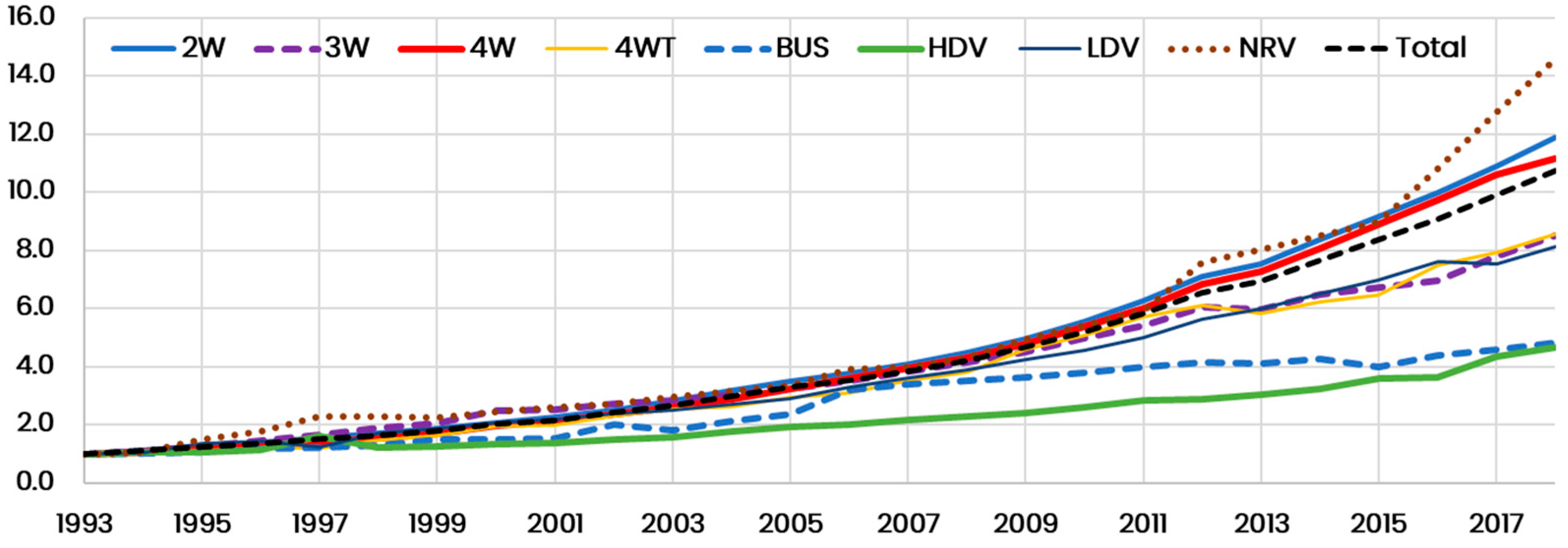
4.1. Registered Vehicle Stock Numbers

Several studies presented an estimate of air and climate pollutant emissions for all India and for Indian cities, but none presented an open database of vehicle stock for replication and further calculations [12,14,22,25,26,27,28,29,30,31,32,33,34,35,36,37]. While the government records publish vehicle stock numbers every year, the databases are not model-ready and require considerable amount of QA/QC. A copy of the official releases is included in the Supplementary Materials.
The total registered number of vehicles (RNV) is calculated using information on the annual sales and/or annual new registrations information, as shown in Equation (3).
R N V v = N V v , g
  • RNV = the number of registered vehicles by vehicle type (v), as reported by MoRTH
  • NV = the number of new vehicles registered every year (by age (g))
RNV refers to the total number of vehicles sold and registered at a regional transport office (RTO) or a city/state, including those in storage, inoperable, or being used infrequently. There are instances when a vehicle is re-sold and re-registered, and the old registration number continues to be in the system, along with the new ownership/registration number [38]. In India, all vehicles are registered for a period of 15 years. There is no prescribed retirement age for vehicles and a provision to re-register for another 15 years can be availed, upon passing safety and environmental checks. In the National Capital Region (NCR) of Delhi, re-registration of diesel vehicles older than 10 years and petrol vehicles older than 15 years is not allowed, which are often transferred to other states for use till their end of life. Typically, when tallying the annual new registrations for RNV, summation over the past 23 years is considered, given the tendency of the vehicles to survive at various maintenance conditions [38,39,40]. It should not be construed that all vehicles under 23 years of age are busy on the roads. The Ministry of Road Transport and Highways (MoRTH) annual reports publish the total number of registered vehicles in the country by state and by city for the categories listed in Table 2 [41]. For convenience, these categories are clubbed into nine broader groups—these groups are often used for emission calculations and evaluation of emission control strategies. A copy of RNV extracts from the MoRTH’s annual report is included in the Supplementary Materials.
Total registered number of vehicles (Table 3) in India touched 300 million in 2018 (as of 31 March 2019—end of India’s financial year 2018). For convenience, only the clubbed categories are presented and discussed in this paper. Of this number, 74.4% were 2-wheelers (2Ws), 13.4% were 4-wheelers (4Ws—including jeeps, sport utility vehicles, and taxis), 0.7% were buses (including intra- and inter-city), 8.4% were freight vehicles (including light- and heavy-vehicles), and 0.7% were non-road vehicles [41]. The total registered vehicles number doubled between 2011 and 2018, increased six times between 2000 and 2018, and increased 11 times between 1993 and 2018 (Figure 1).
Most of the increment comes from the 2W and 4W sectors, mostly due to lack of a similar rate of interest in meeting the travel demand via mass-transit facilities. The total number of buses barely doubled since 2005, while the demand for public transport increased at least 10 times in the same period. For example, a white paper in 1997 on Delhi’s air pollution estimated that the city needs at least 15,000 public transport buses to meet the estimated travel demand in 2000 and the same assessment was made in the clean air action plan proposed under NCAP in 2019–2021, while the city continues to operate less than 4000 buses to meet this demand. The city operated 2000 buses in 1997 [42,43]. The public transportation demand management scenario is similar in other cities. A gradual increase in the demand for total freight vehicles is an indicator of a growing economy, demand for raw and finished products, urbanization with demand for more commercial amenities, and overall gross domestic product of the country [21].
Total registered vehicle estimates by state for select years between 1993 and 2018 is presented in Table 4. This table includes 29 states and 7 union territories (including Delhi). As of 2024, there are 28 states and 8 union territories, with the state Jammu and Kashmir broken into two union territories, with Ladakh added to the list and Dadar and Nagar Haveli and Diu and Daman combined into one union territory. In 2000, three new states were constituted—Chhattisgarh was taken from Madhya Pradesh, Jharkhand from Bihar, and Uttarakhand from Uttar Pradesh. In 2014, the 29th state Telangana was taken from Andhra Pradesh. Vehicle registration numbers for these new states commenced a year after the state’s formation. Till then, their vehicle registration tally is included in that of the old states. States with the largest population also host the largest fleets. As of 31 March 2019, Gujarat, Karnataka, Maharashtra, Madhya Pradesh, Rajasthan, Tamil Nadu, and Uttar Pradesh have more than 15 million RNVs. Delhi, with less than 20 million population (1.5% of the total), has approximately 12 million registered vehicles (4% of the total). The least vehicle density per capita is in the Northeastern states of Assam, Arunachal Pradesh, Manipur, Meghalaya, Nagaland, Sikkim, and Tripura.

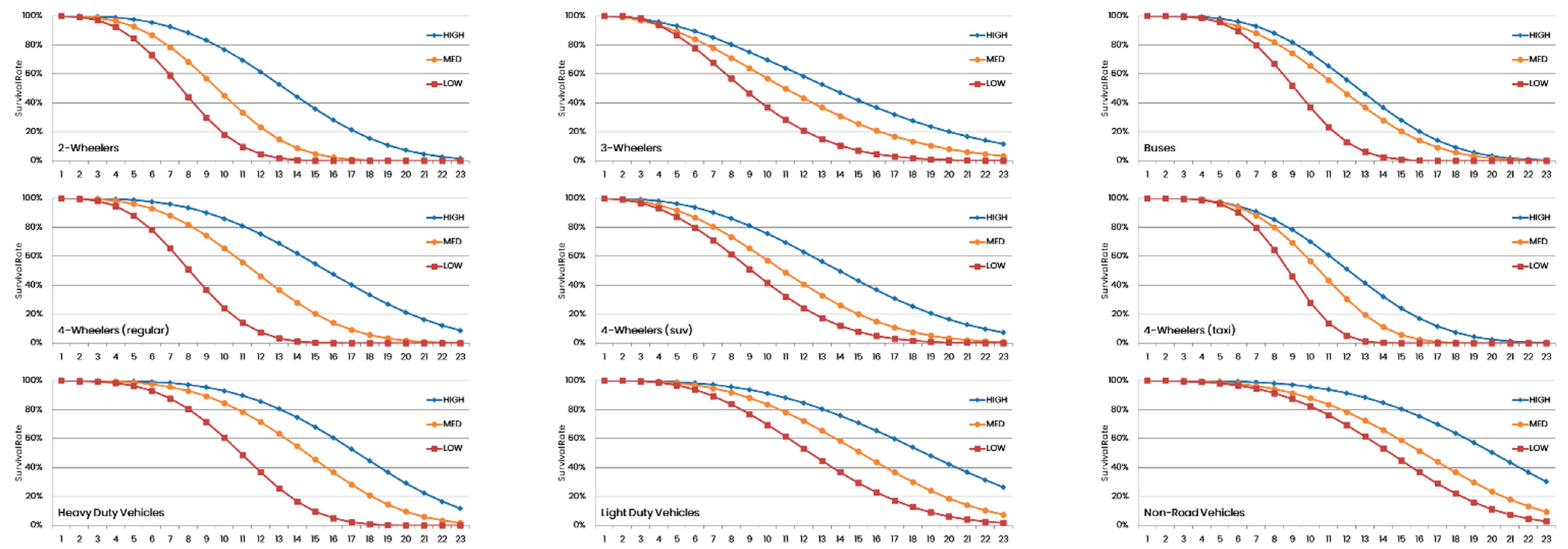
4.2. Survival Functions and In-Use Vehicle Stock Numbers

Equation (4) converts RNV into in-use (or on-road) number of vehicles (INV) using a survival function (SF).
I N V v , g = R N V v , g   S F v , g
  • SF = survival function by vehicle (v)
  • g = age of the vehicle (v)
INV refers to the actual number of vehicles on the roads, driven and used for passenger and freight transportation, and the difference between RNV and INV is significant in India [38]. The MoRTH annual reports refer only to RNV, and the emission calculations (Equations (1) and (2)) must use only INV.
Survival functions (Equation (5)) are used to enable the transition of RNV to INV, for the emissions and pollution models to replicate real world patterns.
S F v = e g + α v T v β v
  • SF = survival function by vehicle (v)
  • g = age of the vehicle
  • T = characteristic service life of the vehicle (v)
  • α, β = shape and scale functions of the SF by vehicle (v)
The survival function model presented here is an adoption of probabilistic Weibull distribution representing the probability of a vehicle still being in-use after a certain number of years [30,40,44,45]. The shape and scale functions (α, β) are summarized in Table 5 and Figure 2 for three different scenarios—high, medium, and low survival rates.
For Tier-1 cities like Bengaluru, Chennai, Delhi, Hyderabad, Kolkata, and Mumbai, low survival functions are applicable, meaning the turnover of the vehicles, especially personal vehicles, is highest in the cities. Similarly, for Tier-2 (medium) cities, like Bhubaneswar, Coimbatore, Indore, Kanpur, Kochi, Ludhiana, Patna, Pune, and Varanasi, medium survival function is applicable. For national level analysis, where it is assumed that a vehicle will survive in any state or till the end of its operational life, the high survival function is applicable. A copy of survival functions for the nine broad categories under the three scenarios and estimated model ready INV information by state is included in the Supplementary Materials. These survival functions (Table 5) are one operational example set based on fuel station surveys conducted in Indian cities [40,46,47] and must be adjusted to represent the vehicle ownership and usage characteristics elsewhere. The characteristic service life of the vehicles (T) is based on the prevalent restrictions on vehicle types. For example, in the Tier-1 cities, passenger 3-wheelers and taxis, after eight years, are required to either retire to other cities or go through stringent maintenance checks to continue to run in the city. Most often, aged vehicles are either run unofficially in a limited capacity or transferred to smaller cities. Lack of stringent inspection and maintenance programs also leads to a gradual drop in a vehicle’s survival probability, after their heavy usage in the initial years. This is also reflected in the drop in vehicle usage (km travelled per day) among aged taxis, passenger 3-wheelers, and freight vehicles [40,48]. For passenger vehicles, the turnover rate is higher in the big cities, which results in a sharp drop-off in aged vehicles, irrespective of any restrictions. For example, the average turnover rate of cars is 4 to 4.5 years in Delhi (low survival) and 6 to 6.5 years in Patna (medium to high survival) [46]. This also translates into a strong second-hand passenger vehicle market in India, and the assumption that, at the national scale, the vehicles are fully utilized in a high survival mode.
An estimated national average age-mix for the in-use fleet using high survival rates is presented in Figure 3. Overall, up to 70% of the fleet tend to be under 10 years of age. The past emission inventory studies indicated that ~20% of the fleet older than 10 years of age includes most of the super-emitters (i.e., vehicles with the highest emission rates) and account for the largest chunk of the total emissions of PM2.5, NO2, CO and VOCs [22,30,39,49,50]. This is often a symptom of poor maintenance of older vehicles.

5. Vehicle Exhaust Emissions Analysis Tools

The fundamental equation for building vehicle exhaust emissions is the multiplication of three parameters—number of vehicles, vehicle km travelled (usage) and an emission factor. When the data are scarce, this equation has versions that can be used to deduce similar emission estimates, with some accountable uncertainty. For example: (a) a method using information on total fuel consumed, share of fuel consumed in various modes, fuel efficiency of the modes, and an emission factor; (b) a method using information on total passenger trips, share of trips in various modes, average trip length of various modes, and an emission factor. An example calculator of these methods is available at https://urbanemissions.info/tools (accessed on 15 May 2024), along with resources to establish representable inputs for use in emissions analysis. These include:
  • A method to convert fleet average speeds and fleet average travel time per day into vehicle km travelled per day.
  • A method to calculate how many additional buses are required to support odd–even or an equivalent scheme (with and without fuel mix exemptions).
  • A method to calculate total fuel wasted from idling in the city and to calculate savings from traffic management.
  • A method to calculate fuel and emission benefits of shifting a share of two-wheeler and four-wheeler trips to buses and non-motorized transport.
  • A method to estimate vehicle exhaust emission factors using emission standards and deterioration rates.
  • An example set of survival rates based on vehicle age for nine broad vehicle categories in Table 5 (to convert yearly RNV into INV).
  • A method to spatially disaggregate (grid) the total vehicle exhaust emissions using multiple grid-level proxies as weights, such as density (km per grid) of various road types, population density, land use/land cover, and information on commercial and industrial activities.
  • A library of emission factors for aerosols and gaseous species.
The evolution of vehicle standards in India is presented in Figure 4. From no norms in late 1990s to introducing Bharat Standard (BS) 6 in 2020, all the new vehicle and fuel standards were introduced in Delhi first, then the metropolitan cities and, after 2–5 years, nationwide. The bifurcated standards had limited effect on reducing the overall emissions, except for in the cities with the new standards, where the passenger vehicles travelling within the city limits benefitted by emitting fewer emissions [39]. In 2020, BS6 was introduced nationwide under the “one nation—one fuel” motto. The overall fleet will take at least 5–8 years, depending on state and city, to host a fleet fraction dominated by BS6 vehicles.
The lack of a single emission factor database in India makes it difficult to accurately estimate, validate, and evaluate the total emissions and the effectiveness of existing emission control policies. A representative sample of emission factor databases available for open use includes: (a) the GAINS (Greenhouse gas and Air pollution Interactions and Synergies) modelling system, which provides a repository of regional level average factors [51]; (b) Central Pollution Control Board (CPCB), New Delhi, India, which provides a repository of emission factors based on a limited series of tests on various vehicle types and age mixes [20]; (c) [32] which, provides a database of emission factors applicable for large cities, derived from a combination of vehicle age-appropriate emission standards and deterioration rates; (d) [52], which provides a database for emission factors for four-wheelers based on tests using on-board testing equipment.

6. Applications and Recommendations

The vehicle stock database presented here is in operational use for an all-India air quality forecasting system (https://indiaairquality.info, accessed on 15 May 2024), which disseminates PM2.5 and other pollutant concentration information for the next three days, along with modelled source apportionment information at state and district level averages. An example of gridded road transport emissions used in the forecasting system and source apportionment results for two states is presented in Figure 5. In addition to the total gridded emissions as an input to the chemical transport model, there are additional corrections considered to simulate realistic conditions, e.g., (a) a reduction in two-wheeler emissions in the grids with rain of more than 0.1 mm per hour; (b) a reduction in the overall road emission loads for the hours and grids with heavy precipitation; (c) zeroing of road dust emissions for the hours and grids with any precipitation. These logical corrections have helped in the evaluation of the inventory at regional and urban scales and attain better confidence intervals when comparing the modelled concentrations with ground measurements in the short-term forecast mode.
The program also includes emissions and pollution analysis for 60 cities under the Air Pollution knowledge Assessments (APnA) program for Indian cities (https://urbanemissions.info/india-apna, accessed on 15 May 2024). The APnA city program is also supporting India’s national clean air program in establishing the layers of information necessary for building an emissions and pollution analysis framework for 131 cities designated as non-attainment areas [15,53,54,55]. A localized emission inventory is necessary for establishing the emission baselines for these cities. Especially for a sector like road transport, which is linked to all the other sectors, delivering raw material, finished products, and people, reliability and replicability of an inventory is important to build confidence in the overall modelling exercise. Additional databases relevant for road transport emissions analysis are available for the designated NCAP urban airsheds (with a spatial resolution of 0.01°, approximately 1 km at https://urbanemissions.info/india-ncap-cities, accessed on 15 May 2024). These include: (a) gridded and geospatial shape files of the road density of primary, secondary, tertiary, and other road types; (b) land use/land cover shares at the grid level, covering urban, barren, agricultural, other vegetation, and water types; (c) gridded urban–rural classification using built-up area extracts from satellite retrievals; (d) gridded multi-year population density; (e) gridded commercial activity density as number of establishments of hotels, hospitals, industries, markets, cinema halls, malls, apartment complexes, and other buildings. These geospatial layers of information can be strategically used for spatial allocation of the total vehicle exhaust emissions calculated using the vehicle stock numbers and as inputs to land use regression models for spatial allocation of information from monitoring networks and surveys.
All the geospatial information layers discussed in this section are global in nature and can be used to replicate similar studies outside India. In addition, the methodologies and models applied for developing emission inventories, conducting air quality forecasting, and evaluating urban air quality are open, with extensive support from the research community as respective model discussion forums.
A new source of vehicle stock information in India includes a new resource, VAHAN, which presents analytics by state and RTO (https://analytics.parivahan.gov.in, accessed on 15 May 2024). However, only the one-time data posted on the portal are public (as of May 2024) and there are no clear guidelines to access the full database at the RTO level for long-term analysis. A recommendation to the authorities is to make the databases open, especially to the academic and research institutions, to sustain these emission calculations and to support urban and regional air quality management programs in India for long-term success. The model-ready information can help in (a) building a long-term emissions inventory for air quality and climate management; (b) evaluation of the emission mitigation strategies at urban and regional scale; and (c) support to urban and national clean air action plans. Example emissions management strategies that can be evaluated using the vehicle stock information are: (a) change in the fuel mix from traditional fuels, like diesel or petrol, to cleaner fuels, like gas or electric; (b) change in the stock age mix with mandated retirements for various vehicle types; (c) change in the stock mix, with restrictions on sales via lottery systems or introducing limits on annual sales; and (d) change in the stock mix with policies restricting vehicle usage based on odd–even registration number.

Supplementary Materials

All the data compiled from the MoRTH annual reports, the cleaned and model ready vehicle stock information for the period covering 1993 to 2018, and a summary of probabilistic survival functions are available at https://doi.org/10.5281/zenodo.11214506 (accessed on 15 May 2024). A copy of MS-Excel based calculators to conduct vehicle exhaust emissions analysis, to build necessary input data and to evaluate scenarios is available at https://www.urbanemissions.info/tools (accessed on 15 May 2024).

Funding

This research received no external funding.

Institutional Review Board Statement

Not applicable.

Informed Consent Statement

Not applicable.

Data Availability Statement

Additional resources are available upon request by email.

Acknowledgments

The analysis and conclusions presented herein are exclusively those of the author and do not represent the supporting organizations or the educational departments.

Conflicts of Interest

The author declares no conflicts of interest.

References

  1. Monks, P.S.; Williams, M.L. What does success look like for air quality policy? A perspective. Philos. Trans. R. Soc. A Math. Phys. Eng. Sci. 2020, 378, 20190326. [Google Scholar] [CrossRef] [PubMed]
  2. Fowler, D.; Brimblecombe, P.; Burrows, J.; Heal, M.R.; Grennfelt, P.; Stevenson, D.S.; Jowett, A.; Nemitz, E.; Coyle, M.; Liu, X.; et al. A chronology of global air quality. Philos. Trans. R. Soc. A Math. Phys. Eng. Sci. 2020, 378, 20190314. [Google Scholar] [CrossRef] [PubMed]
  3. Mądziel, M. Vehicle Emission Models and Traffic Simulators: A Review. Energies 2023, 16, 3941. [Google Scholar] [CrossRef]
  4. Garland, R.M.; Altieri, K.E.; Dawidowski, L.; Gallardo, L.; Mbandi, A.; Rojas, N.Y.; Touré, N.d.E. Opinion: Strengthening research in the Global South–atmospheric science opportunities in South America and Africa. Atmos. Chem. Phys. 2024, 24, 5757–5764. [Google Scholar] [CrossRef]
  5. Crippa, M.; Guizzardi, D.; Butler, T.; Keating, T.; Wu, R.; Kaminski, J.; Kuenen, J.; Kurokawa, J.; Chatani, S.; Morikawa, T. The HTAP_v3 emission mosaic: Merging regional and global monthly emissions (2000–2018) to support air quality modelling and policies. Earth Syst. Sci. Data 2023, 15, 2667–2694. [Google Scholar] [CrossRef]
  6. McDuffie, E.E.; Smith, S.J.; O’Rourke, P.; Tibrewal, K.; Venkataraman, C.; Marais, E.A.; Zheng, B.; Crippa, M.; Brauer, M.; Martin, R.V. A global anthropogenic emission inventory of atmospheric pollutants from sector- and fuel-specific sources (1970–2017): An application of the Community Emissions Data System (CEDS). Earth Syst. Sci. Data 2020, 12, 3413–3442. [Google Scholar] [CrossRef]
  7. Li, M.; Liu, H.; Geng, G.; Hong, C.; Liu, F.; Song, Y.; Tong, D.; Zheng, B.; Cui, H.; Man, H.; et al. Anthropogenic emission inventories in China: A review. Natl. Sci. Rev. 2017, 4, 834–866. [Google Scholar] [CrossRef]
  8. Venkataraman, C.; Brauer, M.; Tibrewal, K.; Sadavarte, P.; Ma, Q.; Cohen, A.; Chaliyakunnel, S.; Frostad, J.; Klimont, Z.; Martin, R.V.; et al. Source influence on emission pathways and ambient PM2.5 pollution over India (2015–2050). Atmos. Chem. Phys. 2018, 18, 8017–8039. [Google Scholar] [CrossRef] [PubMed]
  9. Crippa, M.; Solazzo, E.; Huang, G.; Guizzardi, D.; Koffi, E.; Muntean, M.; Schieberle, C.; Friedrich, R.; Janssens-Maenhout, G. High resolution temporal profiles in the Emissions Database for Global Atmospheric Research. Sci. Data 2020, 7, 121. [Google Scholar] [CrossRef] [PubMed]
  10. Crippa, M.; Guizzardi, D.; Pisoni, E.; Solazzo, E.; Guion, A.; Muntean, M.; Florczyk, A.; Schiavina, M.; Melchiorri, M.; Hutfilter, A.F. Global anthropogenic emissions in urban areas: Patterns, trends, and challenges. Environ. Res. Lett. 2021, 16, 074033. [Google Scholar] [CrossRef]
  11. Solazzo, E.; Crippa, M.; Guizzardi, D.; Muntean, M.; Choulga, M.; Janssens-Maenhout, G. Uncertainties in the Emissions Database for Global Atmospheric Research (EDGAR) emission inventory of greenhouse gases. Atmos. Chem. Phys. 2021, 21, 5655–5683. [Google Scholar] [CrossRef]
  12. Lekaki, D.; Kastori, M.; Papadimitriou, G.; Mellios, G.; Guizzardi, D.; Muntean, M.; Crippa, M.; Oreggioni, G.; Ntziachristos, L. Road transport emissions in EDGAR (Emissions Database for Global Atmospheric Research). Atmos. Environ. 2024, 324, 120422. [Google Scholar] [CrossRef]
  13. Pant, P.; Harrison, R.M. Critical review of receptor modelling for particulate matter: A case study of India. Atmos. Environ. 2012, 49, 1–12. [Google Scholar] [CrossRef]
  14. UEinfo. Air Pollution Knowledge Assessments (APnA) City Program Covering 50 Airsheds and 60 Cities in India. 2024. Available online: https://www.urbanemissions.info (accessed on 15 May 2024).
  15. Ganguly, T.; Selvaraj, K.L.; Guttikunda, S.K. National Clean Air Programme (NCAP) for Indian cities: Review and outlook of clean air action plans. Atmos. Environ. X 2020, 8, 100096. [Google Scholar] [CrossRef]
  16. Yadav, S.; Tripathi, S.N.; Rupakheti, M. Current status of source apportionment of ambient aerosols in India. Atmos. Environ. 2022, 274, 118987. [Google Scholar] [CrossRef]
  17. Venkataraman, C.; Bhushan, M.; Dey, S.; Ganguly, D.; Gupta, T.; Habib, G.; Kesarkar, A.; Phuleria, H.; Raman, R.S. Indian Network Project on Carbonaceous Aerosol Emissions, Source Apportionment and Climate Impacts (COALESCE). Bull. Am. Meteorol. Soc. 2020, 101, E1052–E1068. [Google Scholar] [CrossRef]
  18. Purohit, P.; Amann, M.; Kiesewetter, G.; Rafaj, P.; Chaturvedi, V.; Dholakia, H.H.; Koti, P.N.; Klimont, Z.; Borken-Kleefeld, J.; Gomez-Sanabria, A.; et al. Mitigation pathways towards national ambient air quality standards in India. Environ. Int. 2019, 133, 105147. [Google Scholar] [CrossRef] [PubMed]
  19. Guo, H.; Kota, S.H.; Sahu, S.K.; Hu, J.; Ying, Q.; Gao, A.; Zhang, H. Source apportionment of PM2.5 in North India using source-oriented air quality models. Environ. Pollut. 2017, 231, 426–436. [Google Scholar] [CrossRef] [PubMed]
  20. CPCB. Air Quality Monitoring, Emission Inventory and Source Apportionment Study for Indian Cities; Central Pollution Control Board, Government of India: New Delhi, India, 2011.
  21. Guttikunda, S.; Ka, N. Evolution of India’s PM2.5 pollution between 1998 and 2020 using global reanalysis fields coupled with satellite observations and fuel consumption patterns. Environ. Sci. Atmos. 2022, 2, 1502–1515. [Google Scholar] [CrossRef]
  22. Hakkim, H.; Kumar, A.; Annadate, S.; Sinha, B.; Sinha, V. RTEII: A new high-resolution (0.1° × 0.1°) road transport emission inventory for India of 74 speciated NMVOCs, CO, NOx, NH3, CH4, CO2, PM2.5 reveals massive overestimation of NOx and CO and missing nitromethane emissions by existing inventories. Atmos. Environ. X 2021, 11, 100118. [Google Scholar] [CrossRef]
  23. Ahn, D.; Goldberg, D.; Coombes, T.; Kleiman, G.; Anenberg, S. CO2 emissions from C40 cities: Citywide emission inventories and comparisons with global gridded emission datasets. Environ. Res. Lett. 2023, 18, 034032. [Google Scholar] [CrossRef] [PubMed]
  24. India-PIB. NCAP Targets to Achieve Reductions up to 40% of PM10 Concentrations by 2025–26; Press Information Bureau, Release ID: 1914423; Government of India: New Delhi, India, 2023.
  25. van Aardenne, J.A.; Carmichael, G.R.; LevyIi, H.; Streets, D.; Hordijk, L. Anthropogenic NOx emissions in Asia in the period 1990–2020. Atmos. Environ. 1999, 33, 633–646. [Google Scholar] [CrossRef]
  26. Reddy, M.S.; Venkataraman, C. Inventory of aerosol and sulphur dioxide emissions from India: I—Fossil fuel combustion. Atmos. Environ. 2002, 36, 677–697. [Google Scholar] [CrossRef]
  27. Gurjar, B.R.; van Aardenne, J.A.; Lelieveld, J.; Mohan, M. Emission estimates and trends (1990–2000) for megacity Delhi and implications. Atmos. Environ. 2004, 38, 5663–5681. [Google Scholar] [CrossRef]
  28. Garg, A.; Shukla, P.R.; Kapshe, M. The sectoral trends of multigas emissions inventory of India. Atmos. Environ. 2006, 40, 4608–4620. [Google Scholar] [CrossRef]
  29. Singh, A.; Gangopadhyay, S.; Nanda, P.K.; Bhattacharya, S.; Sharma, C.; Bhan, C. Trends of greenhouse gas emissions from the road transport sector in India. Sci. Total Environ. 2008, 390, 124–131. [Google Scholar] [CrossRef] [PubMed]
  30. Baidya, S.; Borken-Kleefeld, J. Atmospheric emissions from road transportation in India. Energy Policy 2009, 37, 3812–3822. [Google Scholar] [CrossRef]
  31. Ramachandra, T.V.; Shwetmala. Emissions from India’s transport sector: Statewise synthesis. Atmos. Environ. 2009, 43, 5510–5517. [Google Scholar] [CrossRef]
  32. Goel, R.; Guttikunda, S.K. Evolution of on-road vehicle exhaust emissions in Delhi. Atmos. Environ. 2015, 105, 78–90. [Google Scholar] [CrossRef]
  33. Singh, R.; Sharma, C.; Agrawal, M. Emission inventory of trace gases from road transport in India. Transp. Res. Part D Transp. Environ. 2017, 52, 64–72. [Google Scholar] [CrossRef]
  34. Singh, N.; Mishra, T.; Banerjee, R. Emission inventory for road transport in India in 2020: Framework and post facto policy impact assessment. Environ. Sci. Pollut. Res. 2022, 29, 20844–20863. [Google Scholar] [CrossRef] [PubMed]
  35. Dhar, S.; Shukla, P.R. Low carbon scenarios for transport in India: Co-benefits analysis. Energy Policy 2015, 81, 186–198. [Google Scholar] [CrossRef]
  36. Nagpure, A.S.; Gurjar, B.R. Urban Traffic Emissions and Associated Environmental Impacts in India. In Proceedings of the Novel Combustion Concepts for Sustainable Energy Development; Springer: New Delhi, India, 2014; pp. 405–414. [Google Scholar]
  37. Sahu, S.K.; Beig, G.; Parkhi, N. Critical Emissions from the Largest On-Road Transport Network in South Asia. Aerosol Air Qual. Res. 2014, 14, 135–144. [Google Scholar] [CrossRef]
  38. Mohan, D. Moving around in Indian cities. Econ. Political Wkly. 2013, 48, 40–48. [Google Scholar]
  39. Guttikunda, S.K.; Mohan, D. Re-fueling road transport for better air quality in India. Energy Policy 2014, 68, 556–561. [Google Scholar] [CrossRef]
  40. Goel, R.; Guttikunda, S.K.; Mohan, D.; Tiwari, G. Benchmarking vehicle and passenger travel characteristics in Delhi for on-road emissions analysis. Travel Behav. Soc. 2015, 2, 88–101. [Google Scholar] [CrossRef]
  41. MoRTH. Road Transport Yearbook and Statistics Reports for 2000 to 2020; Minister of Road Transport and Highways, the Government of India: New Delhi, India, 2022.
  42. CPCB. White Paper on Pollution in Delhi; Central Pollution Control Board, Government of India: New Delhi, India, 1997. [Google Scholar]
  43. Guttikunda, S.K.; Dammalapati, S.K.; Pradhan, G.; Krishna, B.; Jethwa, H.T.; Jawahar, P. What Is Polluting Delhi’s Air? A Review from 1990 to 2022. Sustainability 2023, 15, 4209. [Google Scholar] [CrossRef]
  44. Zachariadis, T.; Samaras, Z.; Zierock, K.-H. Dynamic modeling of vehicle populations: An engineering approach for emissions calculations. Technol. Forecast. Soc. Chang. 1995, 50, 135–149. [Google Scholar] [CrossRef]
  45. Goel, R.; Mohan, D.; Guttikunda, S.K.; Tiwari, G. Assessment of motor vehicle use characteristics in three Indian cities. Transp. Res. Part D Transp. Environ. 2016, 44, 254–265. [Google Scholar] [CrossRef]
  46. BSPCB. Comprehensive Clean Air Action Plan for the City of Patna; Bihar State Pollution Control Board with Consortium Partners CSTEP, ADRI and Urbanemission.info: Patna, India, 2019. [Google Scholar]
  47. Guttikunda, S.K.; Ka, N.; Tejaswi, V.; Goel, R. Fuel Station Survey (FuSS) to Profile In-Use Vehicle Characteristics for a City’s Vehicle Exhaust Emissions Inventory. Preprints 2024. [Google Scholar] [CrossRef]
  48. Malik, L.; Tiwari, G.; Thakur, S.; Kumar, A. Assessment of freight vehicle characteristics and impact of future policy interventions on their emissions in Delhi. Transp. Res. Part D Transp. Environ. 2019, 67, 610–627. [Google Scholar] [CrossRef]
  49. Sadavarte, P.; Venkataraman, C. Trends in multi-pollutant emissions from a technology-linked inventory for India: I. Industry and transport sectors. Atmos. Environ. 2014, 99, 353–364. [Google Scholar] [CrossRef]
  50. Debbarma, S.; Raparthi, N.; Venkataraman, C.; Phuleria, H.C. Impact of real-world traffic and super-emitters on vehicular emissions under inter-city driving conditions in Maharashtra, India. Atmos. Pollut. Res. 2024, 15, 102058. [Google Scholar] [CrossRef]
  51. GAINS. Greenhouse Gas and Air Pollution Interactions and Synergies (GAINS) by International Institute of Applied Systems Analysis (IIASA), Laxenburg, Austria. 2024. Available online: https://iiasa.ac.at/models-tools-data/gains (accessed on 15 June 2024).
  52. Jaiprakash; Habib, G. On-road assessment of light duty vehicles in Delhi city: Emission factors of CO, CO2 and NOX. Atmos. Environ. 2018, 174, 132–139. [Google Scholar] [CrossRef]
  53. CPCB. National Clean Air Programme (NCAP), Portal for Regulation of Air-Pollution in Non-Attainment cities (PRANA). Available online: https://prana.cpcb.gov.in (accessed on 15 June 2024).
  54. CREA. Tracing the Hazy Air 2023. Progress Report on National Clean Air Programme (NCAP); Centre for Research on Energy and Clean Air: New Delhi, India, 2023. [Google Scholar]
  55. Gupta, M.; Nayak, D.K.; Harsha Kota, S. Impact of Particulate Matter-Centric Clean Air Action Plans on Ozone Concentrations in India. ACS Earth Space Chem. 2023, 7, 1038–1048. [Google Scholar] [CrossRef]
Figure 1. Registered vehicle number growth presented as a ratio of numbers in 1993 (2W, 3W, 4W = all 2–3–4 wheelers; T = taxies; LDV = light duty vehicles; HDV = heavy duty vehicles; NRV = non-road vehicles).
Sustainability 16 06298 g001
Figure 2. Illustration of survival functions for nine broad categories of vehicles in India under three scenarios—high, medium, and low survival rates.
Sustainability 16 06298 g002
Figure 3. Estimated age-mix of India’s in-use vehicle fleet using high survival rates.
Sustainability 16 06298 g003
Figure 4. Timeline of introduction of various vehicle and fuel standards in Delhi and India (source: https://dieselnet.com, accessed on 15 May 2024).
Sustainability 16 06298 g004
Figure 5. (a) Gridded PM2.5 emissions inventory for India at a spatial resolution of 0.25°, established using a combination of total emissions by state and major cities, and a series of geospatial information proxies, such as city airshed sizes, road networks density, population density, and land use/land cover. (b) Example modeled source contributions as all-state average for Delhi and Tamil Nadu from the air quality forecasting system for India using the gridded emissions inventory for all the known anthropogenic and natural sources and modeled meteorological fields at the same spatial and temporal resolution (https://indiaairquality.info, accessed on 15 May 2024).
Sustainability 16 06298 g005
Table 1. Estimated transport and dust contributions in Indian cities, based on emissions-based chemical transport modelling studies for urban airsheds [14].
City (%Transport + %Dust)
Agartala (17.5 + 15.3)Gaya (23.1 + 17.3)Nagpur (17.2 + 10.9)
Agra (13.9 + 10.7)Guwahati-Dispur (36.5 + 27.0)Nashik (12.1 + 13.2)
Ahmedabad (14.9 + 17.7)Gwalior (12.7 + 12.9)Panjim-Vasco-Margao (22.6 + 12.6)
Allahabad (18.6 + 14.9)Hyderabad (16.5 + 18.6)Patna (14.8 + 12.1)
Amritsar-Tarn Taran (10.5 + 7.1)Indore (26.9 + 22.7)Pune-Pimpri-Chinchwad (24.0 + 23.4)
Asansol-Durgapur (12.5 + 16.2)Jaipur (24.1 + 17.5)Raipur-Durg-Bhillai (17.2 + 11.5)
Aurangabad (10.8 + 10.7)Jamshedpur (19.5 + 15.0)Rajkot (19.0 + 16.4)
Bengaluru (26.5 + 23.0)Jodhpur (19.9 + 25.5)Ranchi (21.1 + 14.1)
Bhopal (14.1 + 17.1)Kanpur (13.7 + 8.9)Shimla (17.4 + 11.8)
Bhubaneswar (17.0 + 20.8)Kochi (20.2 + 16.3)Srinagar (9.8 + 8.2)
Chandigarh-Patiala (10.6 + 12.6)Kolkata-Howarh (13.5 + 12.5)Surat (16.4 + 10.3)
Chennai (24.5 + 23.5)Kota (16.7 + 12.5)Thiruvananthapuram (37.0 + 17.4)
Coimbatore (18.3 + 13.7)Lucknow (13.0 + 13.9)Tiruchirapalli (19.0 + 16.2)
Dehradun (14.2 + 4.4)Ludhiana-Phillaur (16.3 + 12.3)Vadodara (20.8 + 17.2)
Dhanbad-Bokaro (12.2 + 29.2)Madurai (23.4 + 19.0)Vijayawada-Guntur (22.7 + 19.7)
Dharwad-Hubli (21.6 + 14.7)Mumbai (16.4 + 12.6)Visakhapatnam (19.3 + 10.9)
Table 2. Vehicle categories listed in the MoRTH annual reports and clubbed category for ease of analysis (2W, 3W, 4W = all 2–3–4 wheelers; T = taxies; LDV = light duty vehicles; HDV = heavy duty vehicles; NNRD = non-road vehicles).
Clubbed CategoryMoRTH Vehicle Categories
12WScooters, mopeds, motorcycles
23WThree wheelers with three, four, and six seaters
34W1Cars
44W2Jeeps and other passenger sports utility vehicles
54WTTaxi motor cabs, maxi cabs, and others
6BUSOmni buses, stage carriages, contract carriages, private service vehicles, and others
7LDVThree and four-wheeler goods carriages
8HDVMulti-axle vehicles, trucks, and lorries
9NNRDTractors, trailers, and other non-road vehicles
Table 3. 1993–2018 total registered vehicle fleet (in millions) in India (2W, 3W, 4W = all 2–3–4 wheelers; T = taxies; LDV = light duty vehicles; HDV = heavy duty vehicles; NRV = non-road vehicles).
2W3W4W4WTBUSHDVLDVNRVTotal
199318.30.83.30.30.42.11.80.127
199420.80.93.50.40.42.31.90.230
199523.31.03.80.40.42.22.50.234
199625.71.24.20.40.52.42.70.337
199728.41.34.60.40.53.42.30.341
199831.31.55.00.50.52.63.20.345
199934.11.65.50.60.62.73.50.349
200038.62.06.40.70.62.93.90.456
200141.82.07.00.70.62.94.10.459
200246.82.27.70.80.83.24.50.466
200351.92.38.50.90.83.34.70.473
200458.82.59.40.90.93.85.10.582
200564.72.610.51.01.04.15.50.590
200669.12.811.61.11.44.36.20.697
200775.43.112.81.31.44.66.70.6106
200882.43.414.01.41.54.97.30.7115
200991.63.615.51.61.55.17.90.7128
2010101.94.017.51.81.65.58.60.8142
2011115.54.419.62.01.76.09.40.9159
2012133.24.922.92.21.86.210.71.1183
2013141.54.824.32.11.86.511.31.2194
2014156.75.226.92.31.86.912.31.3214
2015171.75.529.72.41.77.713.21.3233
2016187.25.732.52.71.97.714.41.6254
2017204.46.335.42.91.99.314.31.9276
2018223.06.937.33.12.110.015.32.2300
2018%74.4%2.3%12.4%1.0%0.7%3.3%5.1%0.7%
Table 4. 1993–2018 (for select years) total registered vehicle fleet (in millions) by state.
1993199520002005201020152018
Andaman and Nicobar Islands0.010.010.030.030.070.110.14
Andhra Pradesh1.612.584.057.2210.198.5311.67
Arunachal Pradesh0.010.020.020.020.140.260.23
Assam0.350.360.550.911.582.853.97
Bihar1.221.330.971.452.675.488.55
Chhattisgarh 0.861.542.774.816.38
Chandigarh0.310.370.390.651.020.841.02
Diu and Daman0.010.020.040.060.080.110.12
Delhi2.282.683.554.507.249.9411.40
Dadar Nagar Haveli0.010.010.010.050.080.110.00
Goa0.180.210.340.530.771.131.40
Gujarat2.733.385.608.6212.9920.3625.20
Himachal Pradesh0.090.120.220.330.621.181.63
Haryana0.841.071.993.095.418.6811.43
Jharkhand 0.911.513.113.354.30
Jammu Kashmir0.160.200.330.520.931.371.82
Karnataka1.812.253.566.229.8216.1520.90
Kerala0.891.172.153.765.9810.0913.25
Lakshadweep0.000.000.000.010.010.020.02
Maharashtra3.274.036.8811.0217.5027.8735.39
Meghalaya0.040.040.060.100.180.290.37
Manipur0.050.060.080.120.210.310.36
Madhya Pradesh1.892.313.104.617.3611.9815.30
Mizoram0.020.020.030.050.090.170.26
Nagaland0.080.100.170.200.290.380.49
Odisha0.540.661.111.943.345.838.28
Punjab1.641.922.924.045.279.6010.61
Puducherry0.110.130.250.380.670.861.06
Rajasthan1.441.772.964.757.9913.6417.72
Sikkim0.010.010.010.020.040.050.07
Tamil Nadu2.152.775.1710.0515.6424.2030.18
Tripura0.030.030.050.110.190.330.50
Telangana 8.8212.50
Uttarakhand 0.370.641.001.892.75
Uttar Pradesh2.482.994.917.9913.2923.9432.71
West Bengal1.011.241.892.873.267.617.80
Table 5. Survival function parameters for nine broad categories of vehicles in India under three scenarios—high, medium, and low survival rates.
ClubbedAβT
CategoryLowMediumHighLowMediumHighLowMediumHigh
12W0.50.30.13.13.13.181014
23W−1.00.00.02.02.02.081215
34W10.00.0−0.53.03.03.081216
44W20.50.50.02.52.52.5101215
54WT−0.5−0.5−0.54.03.53.081012
6BUS−1.00.0−1.03.23.03.081212
7LDV−1.00.00.02.53.03.0121620
8HDV1.01.00.03.83.83.8121618
9NNRD1.01.01.03.53.54.0161822
Disclaimer/Publisher’s Note: The statements, opinions and data contained in all publications are solely those of the individual author(s) and contributor(s) and not of MDPI and/or the editor(s). MDPI and/or the editor(s) disclaim responsibility for any injury to people or property resulting from any ideas, methods, instructions or products referred to in the content.

