Abstract
Accurately estimating the state of health (SOH) of lithium-ion batteries ensures the proper operation of the battery management system (BMS) and promotes the second-life utilization of retired batteries. The challenges of existing lithium-ion battery SOH prediction techniques primarily stem from the different battery aging mechanisms and limited model training data. We propose a novel transferable SOH prediction method based on a neural network optimized by Harris hawk optimization (HHO) to address this challenge. The battery charging data analysis involves selecting health features highly correlated with SOH. The Spearman correlation coefficient assesses the correlation between features and SOH. We first combined the long short-term memory (LSTM) and fully connected (FC) layers to form the base model (LSTM-FC) and then retrained the model using a fine-tuning strategy that freezes the LSTM hidden layers. Additionally, the HHO algorithm optimizes the number of epochs and units in the FC and LSTM hidden layers. The proposed method demonstrates estimation effectiveness using multiple aging data from the NASA, CALCE, and XJTU databases. The experimental results demonstrate that the proposed method can accurately estimate SOH with high precision using low amounts of sample data. The RMSE is less than 0.4%, and the MAE is less than 0.3%.
1. Introduction
Due to their wide operating temperature range, convenient charging capabilities, low self-discharge rate, and environmental friendliness, Lithium-ion batteries (LIBs) have been widely adopted in electric vehicles (EVs) and distributed energy storage systems. This transition effectively reduces carbon emissions and fossil energy consumption. The internal structure of a battery changes as a result of an increasing number of usage cycles and improper charging and discharging practices. The presence of internal resistance, capacity degradation, voltage fluctuations, and other effects can negatively impact the device’s performance and safety. The state of health (SOH) of a battery represents the performance of the active materials and electrolytes within the battery. Variations in this parameter can indicate changes in the internal health state of a battery [1]. Battery performance declines rapidly if the capacity drops below 80% of its initial capacity [2], resulting in power devices being unable to operate or becoming permanently damaged. In certain applications, the battery may be deemed unusable when its SOH reaches 70–80% of its rated capacity. Therefore, an accurate assessment of battery health status is required to ensure that battery management systems (BMSs) operate normally, preventing accidents. Moreover, evaluating the health status of retired batteries can facilitate their reuse in secondary applications, extend their life cycle, and minimize resource waste [3].
Various methods have been suggested for assessing the degree of battery degradation and aging based on the SOH of a battery. Research on predicting lithium-ion batteries’ health status has incorporated a number of innovative methods and techniques. Advances in technology have improved the accuracy of predicting LIB health status, which is beneficial to the long-term maintenance and safe operation of these batteries. SOH estimation methods are currently divided primarily into two categories: model-based estimation and data-driven estimation [4]. The model-based estimation method constructs a model that describes the aging behavior of LIBs through a series of algebraic and differential equations. Then, it is used to identify the battery aging parameters using filtering algorithms and their derived algorithms to achieve SOH estimation. According to different model mechanisms, the model-based methods can be divided into electrochemical models and equivalent circuit models (ECMs) [5]. The electrochemical model derives mathematical formulas, such as differential or partial differential equations, that characterize the battery performance decay mechanism by analyzing the lithium-ion battery’s internal composition and working principle. The electrochemical model has high accuracy, but complexity needs to be lowered in actual SOH estimation [6]. The ECM ignores the above physical and chemical reactions and approximates the aging behavior of the battery by using existing circuit components such as resistors and capacitors. Analyzing experimental data achieves accurate model-related parameter identification. However, due to the fixed structure of the ECM, it is challenging to achieve high-precision SOH estimation for the entire life cycle of the battery [7].
One major limitation of model-based methods is that if the model selected does not accurately reflect the physical and chemical processes of the battery, the SOH estimation results will be inaccurate. Furthermore, capturing all potential battery degradation mechanisms and reflecting them in model parameters is challenging. Unlike model-based SOH estimation methods, data-driven estimation methods do not require a deep understanding of the complex degradation mechanism inside the battery. Data-driven methods can automatically establish the mapping relationship between the battery-aging features contained in a large amount of battery charging and discharging data and SOH. Data-driven methods are easy to operate and have high estimation accuracy and generalization ability. Support vector regression (SVR) [8], Gaussian process regression (GPR) [9], neural networks (NNs) [10], and Ensemble learning [11] are very powerful and have been widely applied. Li et al. [12] directly used the original voltage data of the constant current stage charging curve as input to the LSTM-RNN network. The network shows excellent anti-interference and estimates SOH ability when facing input noise. Tagade et al. [13] used local charge and discharge time series data (voltage, current, and temperature) based on deep GPR for capacity estimation without extracting additional input features to achieve high prediction accuracy. However, the features automatically extracted by these methods often need a more precise physical meaning.
Nowadays, feature-processing methods are widely used because they simplify and reduce computation time by extracting health features (HFs). Feature processing refers to the extraction of trends from collected data, such as voltage, current, and temperature, from batteries. The purpose of this analysis is to characterize the aging performance of LIBs. An explanation-boosting machine was used by Lin et al. [5] to estimate the SOH, which improved accuracy and robustness when the battery was near its end of life due to the battery’s internal resistance. In the work by Wang et al. [14], 12 HFs were extracted from the incremental capacity curve and input to a structurally weighted twin SVR model in order to assess SOH accurately. Feng et al. [15] utilized an improved GPR method to estimate SOH and remaining life based on 5 HFs calculated from the charging current curve of the battery. Zhang et al. [16] extracted 25 statistical characteristics of feature histograms from the original data collected under different operating conditions and used them as features to learn battery aging. Roman et al. [17] proposed a SOH estimation method based on machine learning to extract 30 features from the battery charging curve. Thermal runaway presents a significant risk to lithium battery operation; thus, temperature is strongly correlated with the SOH. Based on the accelerated durability test with idle and load-changing cycles and the degradation characteristics test, Tang et al. [18] established a mathematical model that reveals the relationship among load current, SOH, and optimal temperature reference. With the assistance of domain knowledge, enhanced features can be constructed using original data to extract more practical information, which can be used to describe battery aging more effectively. Then, statistical analysis, correlation analysis, and other methods can be utilized to identify the most representative and predictive features, which will enhance the model’s accuracy and generalization capability.
The degradation of LIBs typically manifests as a decline in battery capacity and partial recovery with increasing charge-discharge cycles, which may be referred to as a time series problem. SOH has been successfully diagnosed using recurrent neural networks (RNNs), which are particularly suited to processing sequential data [19]. The problem of vanishing or exploding gradients makes it difficult for RNNs to capture long-term dependencies. LSTM is an improved variant of the standard RNN, which effectively captures the long-term trend of decreasing battery capacity over time [20]. In the design and training of LSTM models, the number of neurons is a crucial factor that influences the model’s complexity and fit. The predictive power of LSTM cannot be fully exploited through empirical parameter selection. The model may be unable to capture complex patterns in the data if its neurons are too small, resulting in insufficient fitting ability. Alternatively, overfitting may occur when there are too many neurons, which will result in poorer predictive ability. Designing and training LSTM models requires balancing model complexity and predictive accuracy with the appropriate number of neurons. Qian et al. [21] proposed a method to estimate battery capacity using a one-dimensional convolutional neural network (CNN). The neural network hyperparameters were optimized by using a linear decreasing weighted particle swarm optimization algorithm, resulting in accurate battery capacity estimation. Li et al. [22] proposed a method for SOH estimation that uses the improved ant lion optimization (IALO) algorithm to optimize the kernel parameters of SVR. This method has been demonstrated to be highly accurate and robust in experimental studies. With random battery data length inputs, Zhang [23] proposed a method for estimating SOH that optimizes back propagation (BP) of neural networks using genetic algorithms (GAs). Harris hawk optimization (HHO) is widely used due to its simple structure, fast convergence, and strong local search performance. Jafari [24] proposed an innovative method combining HHO to optimize random forest and LightGBM hyperparameters, accurately estimating the battery’s remaining useful life (RUL). Gadekallu [25] proposed a hybrid HHO-CNN model for gesture image classification. HHO is used to adjust CNN hyperparameters, and the proposed model achieved 100% accuracy.
Battery health prediction is challenging due to nonlinearity, wide operating conditions, and different aging processes. Furthermore, deep learning requires an extensive amount of training data, limiting the application space for LIB SOH estimation. Using knowledge derived from different but related source domains could improve the performance of data-driven methods in the target domain [26]. Deng et al. [27] used early aging data of batteries to achieve aging pattern recognition and transfer learning (TL), effectively improving SOH estimation accuracy. Yao et al. [28] used the capacity increment features of partial charge/discharge data and adopted a deep transfer convolutional neural network to improve battery capacity estimation accuracy. Che et al. [29] developed an innovative method for predicting RUL based on gated RNNs and TL. TL can leverage data from the source domain to reduce the model’s demand for data from the target domain.
Although deep learning and optimization algorithms have achieved certain results in battery health prediction, they still have some limitations. Deep learning requires a large amount of training data, which may be difficult to obtain in practical applications. Optimization algorithms can adjust the hyperparameters of the model to improve prediction accuracy, but these methods often require a large amount of computational resources and may lead to model overfitting. In order to address these challenges, this paper proposes a new method that utilizes features extracted from the voltage, current, and temperature profiles of LIBs during charging. These features not only contain the physical information of the battery but can also be obtained from actual charging data. They serve as inputs for the base model LSTM-FC and allow the model to be transferred to different application scenarios. During the transfer, a fine-tuning strategy is adopted without modifying the model structure. In order to ensure the precision and generalizability of both the base and transfer models, we employ the HHO algorithm for the global optimization of the hyperparameters in our proposed model. This method can not only reduce the demand for data in the target domain but also improve the accuracy and generalization ability of SOH estimation. According to the experimental results, the proposed method can enhance estimation accuracy while maintaining high stability.
While specific experiments on retired batteries have not been conducted yet, our method is highly suitable for their assessment. By utilizing transfer learning, our approach accurately estimates the SOH of batteries even with limited sample data. This capability has substantial potential for evaluating the health status of retired batteries, thereby enabling their reuse in secondary applications. Such practices contribute to a circular economy and sustainable development by optimizing resource utilization and minimizing environmental impact.
The remainder of this paper is organized as follows: Section 2 presents the extraction of degradation features based on the charging curve. Section 3 describes the LSTM-FC base model, the HHO optimization algorithm, and the proposed SOH prediction method. Section 4 introduces the experimental results and analysis. Section 5 provides the conclusion.
2. Health Feature Extraction
Data-driven methods include data preprocessing, feature selection, model training, and others. Improvements in each of these steps can enhance predictive capabilities. In particular, in predicting capacity loss, selecting battery data features significantly impacts accuracy [30,31]. Feature data and output labels must be correlated in order for the model to be accurate. The prediction model will become more accurate as the correlation increases. We conducted a Spearman correlation analysis to verify the effectiveness of the extracted parameters in this section, which extracts features that effectively represent the aging characteristics of LIBs.
2.1. Definition of SOH
The SOH of a battery is a vital indication that represents the extent of LIB degradation. The battery’s SOH can be defined as any factor that characterizes its health status [32]. Most current research defines SOH using battery aging characterization parameters such as capacity, internal resistance, and power. However, these characterization parameters are not the only determinants of battery health, as some internal parameters also reflect health status. The capacity indicator is the most commonly used indicator, as shown in Equation (1).
where and represent the rated capacity and current capacity, respectively, and the SOH of a new battery is 100%. Changes in usage time and environment modify the battery’s internal materials and structure, resulting in a decrease in SOH.
2.2. Lithium-Ion Battery Aging Test Dataset
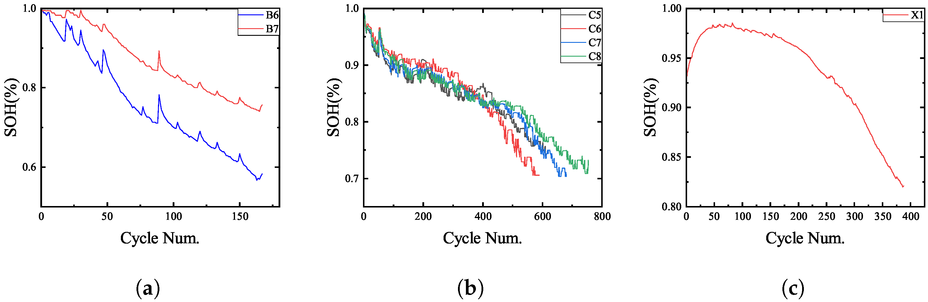
The NASA Prognostics Center of Excellence (PCoE) provided the first experimental data for this experiment [33], including batteries B0006 (B6) and B0007 (B7). The batteries utilize LiCoO2/LiNiCoAlO2 as the cathode material and have a rated capacity of 2 Ah. At a temperature of 24 °C, the batteries were subjected to a continuous flow of electric current of 0.75 C until the batteries’ voltage reached 4.2 V. After that, the batteries were charged at a constant voltage of 4.2 V until the charging current dropped below 20 mA. Batteries B6 and B7 were discharged at a constant current of 1 C until their voltages dropped to 2.5 V and 2.2 V, respectively. Figure 1a shows degradation data for two batteries.

Figure 1.
SOHvariation curve of the battery dataset. (a) NASA; (b) CACLE; (c) XJTU.
The second set of experimental data comes from the CALCE battery dataset provided by the University of Maryland [34]. This includes batteries CS2_35 (C2), CS2_36 (C6), CS2_37 (C7), and CS2_38 (C8). The batteries’ cathode material is LiCoO2, and it has a 1.1 Ah capacity. The batteries underwent charging at a consistent current of 0.5 C until the voltage reached 4.2 V. Subsequently, they were recharged at a voltage of 4.2 V until the charging current dropped below 50 mA. The voltage of all four batteries was reduced to 2.7 V by discharging them at a steady 1 C current. Figure 1b shows the deterioration data for the four batteries.
The third set of experimental data is derived from the XJTU battery dataset, which is provided by Xi’an Jiao Tong University [35]. This study focuses solely on the first battery (X1) from batch 1. The battery’s chemical composition is LiNi0.5Co0.2Mn0.3O2, and it has a nominal capacity of 2 Ah. The battery was charged to 4.2 V at room temperature using a constant current of 2 C. The voltage was then maintained until the current dropped to 0.05 C. After a rest period of 5 min, the battery was discharged at 1 C until it reached 2.5 V, followed by another 5-minute rest period. Figure 1c presents the deterioration data for this battery.
2.3. Health Feature Extraction Based on Charging Curve
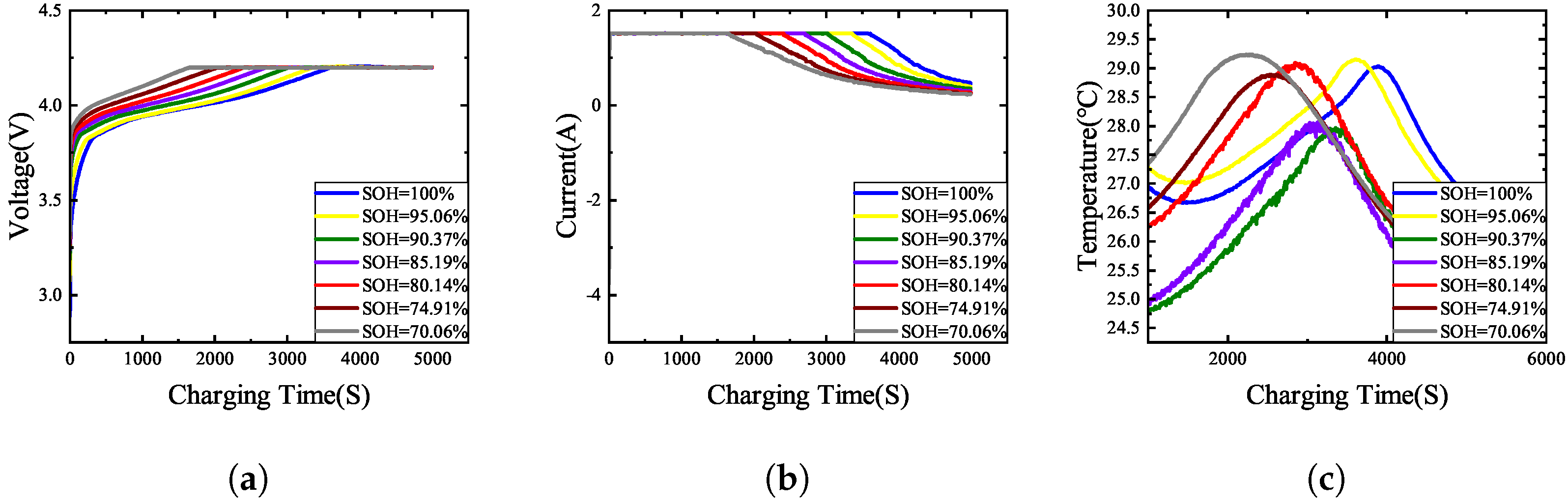
The charging data are more accessible and relevant to time than the uncertain discharge process. Considering the feasibility of online applications, we only extracted aging features based on the battery charging stage. Figure 2 illustrates the charging voltage and current curve for B6. The constant current charging time decreases as SOH decreases, while the average constant current charging voltage gradually increases. This paper selects four indirect health features: the proportion of constant current charging time (F1), the average value of constant current charging voltage (F2), the charging capacity (F3), and the time to reach maximum temperature (F4), respectively. The charging capacity (F3) is calculated based on Coulomb counting.

Figure 2.
Partial charging curves of battery B6 under different SOH states. (a) Charging voltage; (b) charging current; (c) charging temperature.
2.4. Spearman Correlation Analysis
The effectiveness of the extracted features was evaluated using Spearman correlation analysis [36].
where represents the spearman correlation coefficient. and correspond to feature values and battery SOH, respectively, while and are their averages. As approaches 1, the correlation between x and y becomes stronger. Table 1 below provides a quantitative correlation analysis between the proposed features and SOH. The CALCE dataset does not have temperature data. The health features extracted from the dataset have a strong correlation with SOH.

Table 1.
Spearman correlation coefficients.
3. Methodology
A novel transferable SOH prediction method based on LSTM-FC and optimized by the HHO algorithm is presented in this section. We introduce an LSTM-FC framework for modeling battery aging data, where the LSTM layer can learn the long-term degradation trend of LIBs; the FC layer can further learn and fuse features and also serves as a “firewall” for target domain transfer learning. The HHO algorithm improves the accuracy and transferability of LSTM-FC by optimizing the units of hidden layers and training epochs.
3.1. LSTM-FC
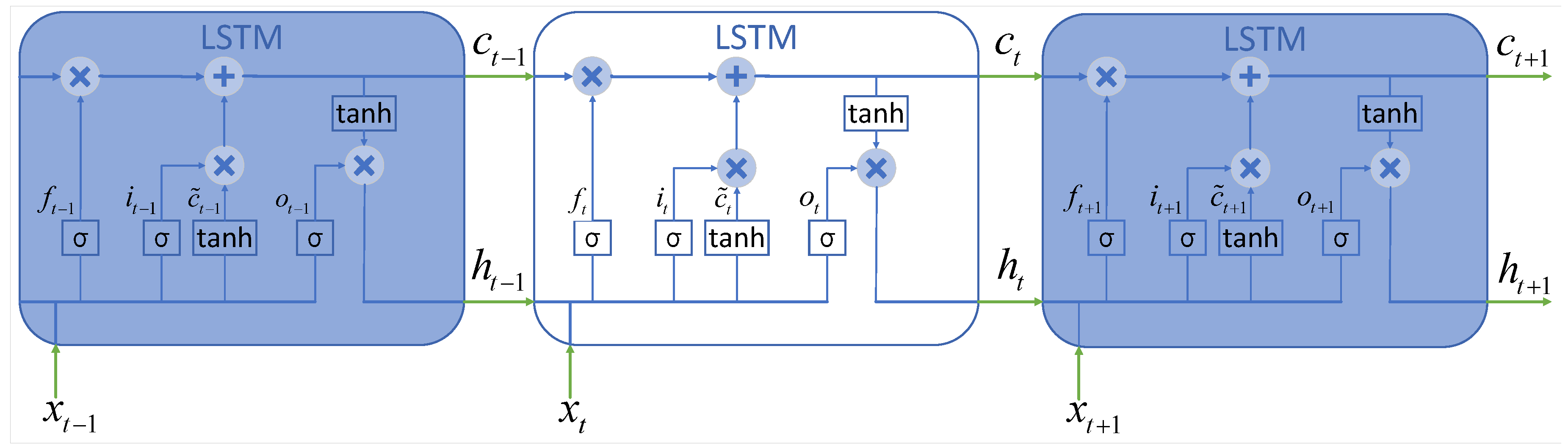
LSTM was introduced to address the issues of slow gradient updates due to the vanishing gradients of RNNs and the slow network parameter optimization process due to exploding gradients [37]. When we use LSTM for SOH estimation, a typical dataset is , where and are the actual SOH value and input feature vector at the cycle step n, respectively. LSTM consists of a series of recurrent neurons, as shown in Figure 3. The core idea of LSTM is to control the flow and retention of information through gate units. LSTM includes three critical gate units: the forget gate, the input gate, and the output gate. These gate units are responsible for controlling the flow of information and updating the memory state, meeting the conditions for the dynamic updating of cyclic weights.

Figure 3.
The framework of the LSTM neural network.
Each LSTM unit accepts the hidden state and cell state from the previous time step and forwards the current time step’s hidden state and cell state to the following LSTM unit. Compared to RNN, LSTM has an additional current time step cell state to pass memory information. Among them, is used for output or is passed to the next step; contains memory information from the previous steps and updated information from the current time step. LSTM introduces a gate structure to decide which information can be sent to the next LSTM unit.
The forget gate, , receives inputs and (the current time step’s input) and determines which information in the previous cell state should be forgotten by using an activation function (usually a sigmoid function).
In the formula, is the hyperbolic sigmoid function, is the weight matrix of the forget gate, and is the bias matrix.
The input gate takes and as inputs. A gate structure and the tanh function determine the degree of influence of the current input on the update of the cell state. This controls the amount of input information added to the cell state.
For the input gate, and represent the weight matrices, and and represent the bias matrices.
According to Equations (3)–(5) and Figure 3, the updated formula for the cell state is as follows:
The output gate also accepts the inputs and . Equation (8) shows the calculation formula for the hidden state based on the cell state and the output gate:
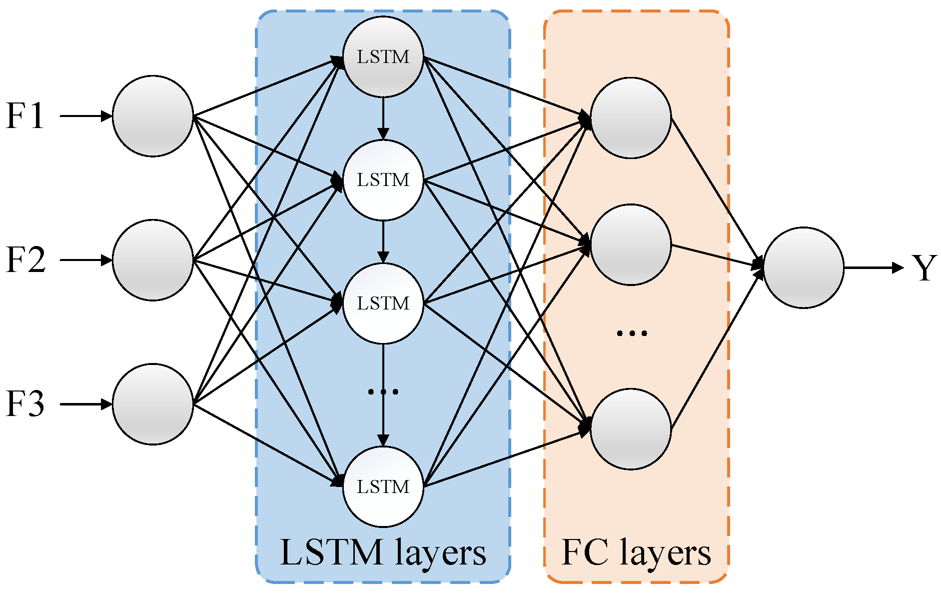
Different lithium batteries exhibit different aging and degradation processes. The LSTM is capable of understanding and storing long-term trends in battery degradation. The gate mechanism makes LSTM an effective tool for analyzing time-series data. With the output of the LSTM layer fed into the fully connected (FC) layer, the feature space can be transformed for improved classification. The FC layer serves not only as a feature extraction layer but can also serve as a “firewall” for the transfer of features into the target domain [38]. Ultimately, the basic model is designed as one LSTM layer plus one FC layer, as shown in Figure 4.

Figure 4.
LSTM-FC network structure.
3.2. Harris Hawk Optimization
HHO is a swarm optimization algorithm proposed by Heidari et al., which mimics the predatory behavior of Harris hawks. Three stages are involved in the process: global exploration, transition, and exploitation [39]. During exploitation, the hawks employ four strategies to capture the rabbit (representing the optimal solution).
3.2.1. Global Exploration Phase
Harris hawks are distributed randomly and discover prey based on two equally probable strategies. The specific model is as follows:
where represents the hawk’s position; is the rabbit’s position; , , , , and p are random numbers within (0, 1), which are randomly assigned in each iteration; and are the upper and lower bounds of the optimization variables, respectively; is a randomly selected hawk; and is the average position of the current hawk population.
By using Equation (10), we can determine the average position of the hawk:
where represents the position of each hawk during the iteration process; N is the total number of hawks in the swarm.
3.2.2. Transition Phase
The energy of the prey significantly decreases during the escape process, and its escape energy is modeled as follows:
where E is the energy of the prey’s escape; is the prey’s initial energy, which is a random number between (−1, 1); and T is the maximum number of iterations.
During the iteration process, the escape energy E continues to decrease. When the escape energy , the HHO algorithm enters the global exploration stage. Otherwise, it enters the local exploitation stage.
3.2.3. Exploitation Phase
In the HHO algorithm, the factor describes whether the hawk successfully captures the prey: when , it indicates a failed capture; when , it indicates a successful capture. At the same time, the Harris hawk adopts different encirclement strategies based on the relative size of the prey’s escape energy E and 0.5.
- Soft besiege: When and , it indicates that the prey’s energy E is sufficient and attempts to escape the encirclement by randomly jumping but ultimately fails and is captured. The position of the Harris hawk is updated as follows:where is the distance between the hawk and the prey; is the prey’s random jumping ability when escaping; and .
- Hard besiege: When and , it indicates that the prey’s energy E is low, and the prey is directly captured. The position is updated as follows:
- Soft besiege with progressive rapid dives: When and , it indicates that the prey’s energy E is sufficient, ensuring successful escape. However, the hawk swoops down in the optimal direction to softly encircle and capture the prey, and its position is updated as follows:Then, the process compares the results with the previous ones. If Y is not reasonable, they will swoop down in a pattern based on Levy’s flight when approaching the rabbit, and the position is updated as follows:where S is a D-dimensional random vector, and is a D-dimensional Lévy function; the formula is as follows:where u and v are random numbers within (0, 1), .Therefore, the final strategy can be executed by using Equation (18).
3.3. Transfer Learning
By utilizing machine learning techniques to construct appropriate data-driven models, the precise estimation and aging prediction of specific battery conditions can be achieved. However, the complex degradation patterns of batteries caused by different working conditions pose significant challenges to the practical application of these methods. Transfer learning is a method that enhances the performance of data-driven models by transferring knowledge from related domains. It will become an effective means of intelligent battery management if used correctly. Transfer learning can apply knowledge from other related tasks to the target task. This avoids learning new tasks from scratch and reduces the need for large amounts of data for the target tasks. In battery management applications, the primary methods used for battery state estimation and aging prediction include feature-based transfer learning (feature-based TL) and parameter-based transfer learning (parameter-based TL) [26,40]. Feature-based transfer learning is achieved by applying a domain adaptation strategy, while parameter-based transfer learning is achieved through a fine-tuning strategy.
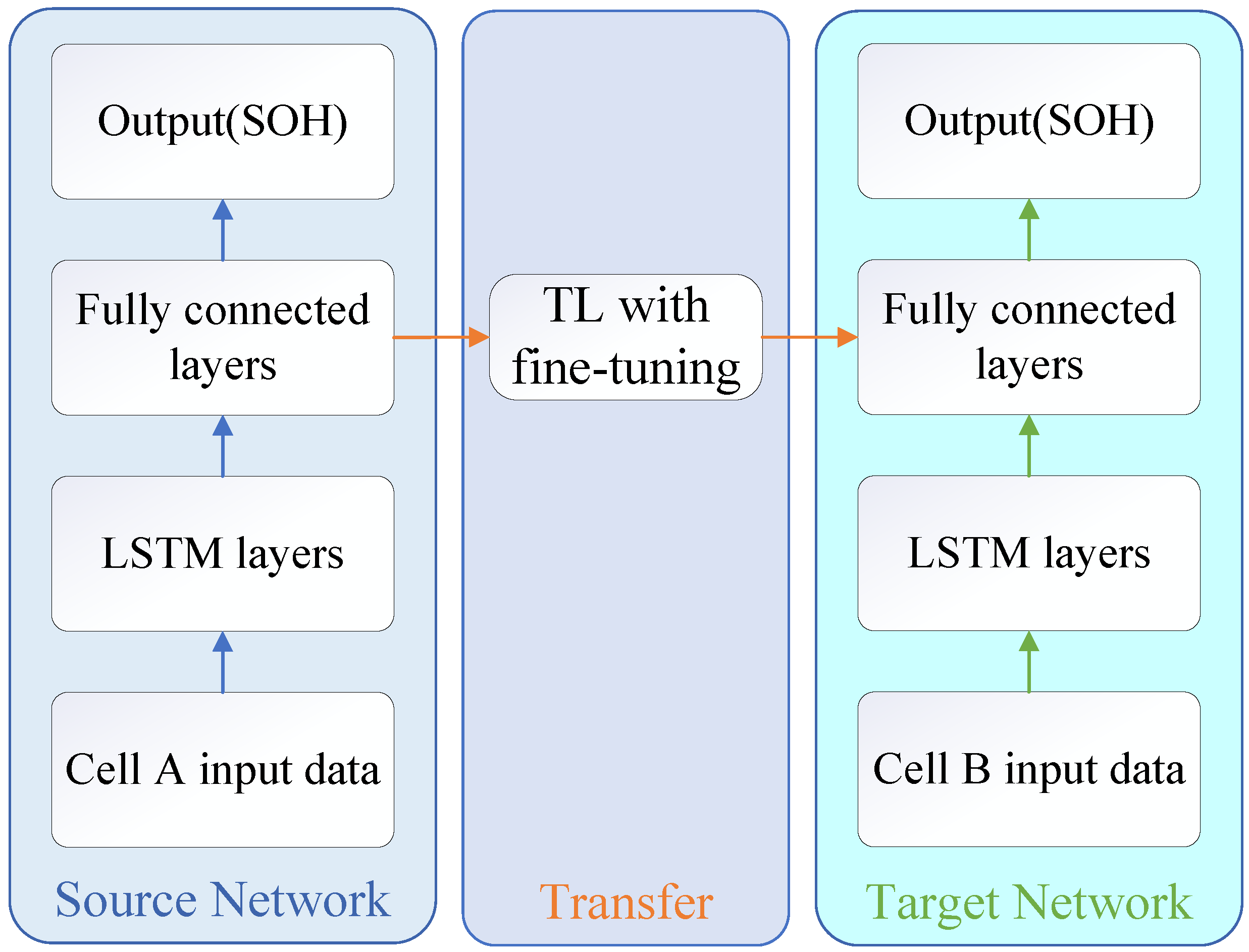
This paper uses parameter-based transfer learning, as shown in Figure 5. The core concept is to retrain the already trained basic data-driven model by introducing new data from different environments to adapt to the state estimation scenario of LIBs in the new application environment.

Figure 5.
The network structure of the parameter-based transfer learning.
3.4. HHO-LSTM-FC-TL Model
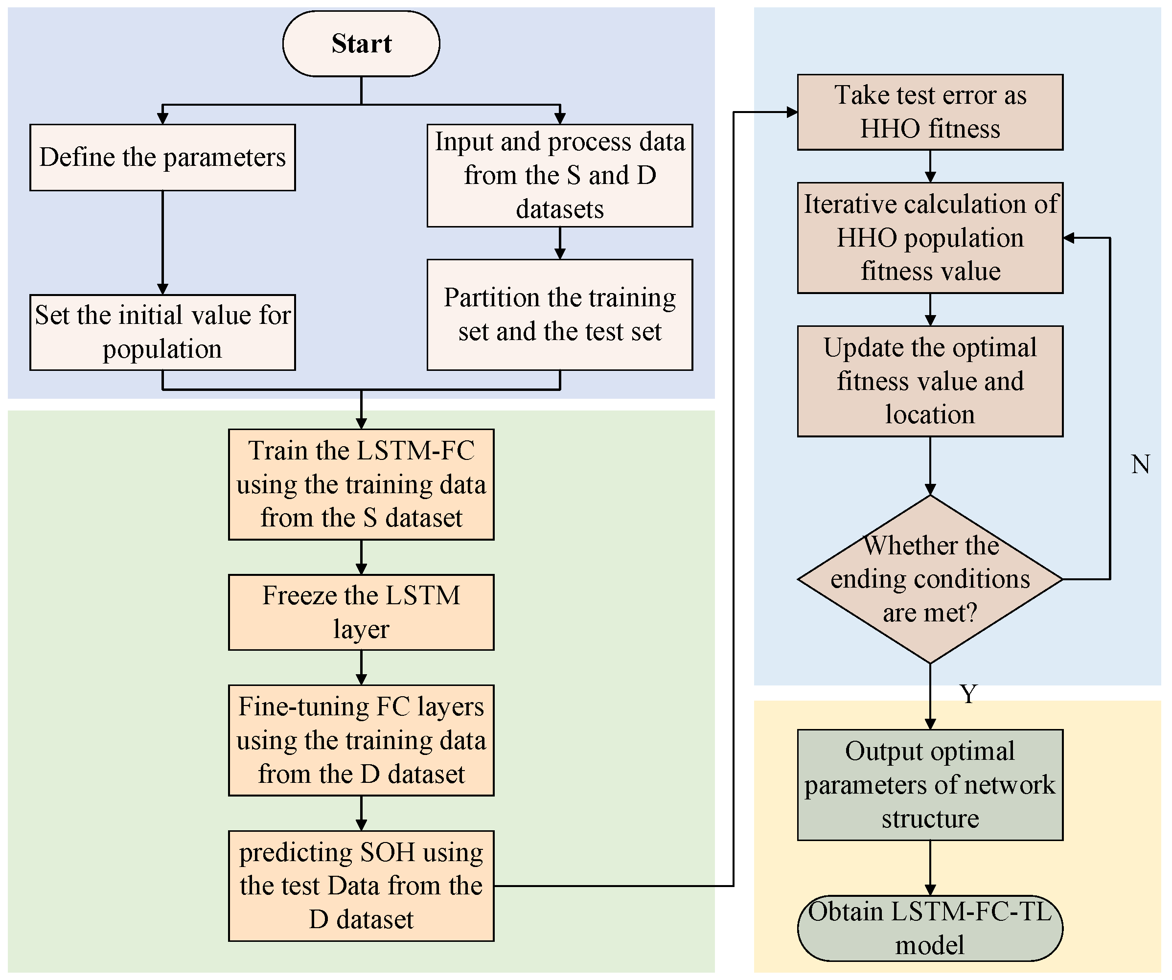
The number of iterations and hidden layer units is crucial for training LSTM. By increasing the number of epochs, the model has more opportunities to learn patterns and features from the dataset. However, too many epochs may lead to overfitting the training data, increasing generalization error. Complex models with many hidden layers can capture more complex patterns. However, this also means more computational resources are needed. Therefore, the hidden layer units must be adjusted according to the dataset size. The HHO algorithm has shown significant superiority in global parameter optimization due to having few parameters, fast convergence speed, high stability, and ease of implementation. The HHO can effectively avoid local optimal solutions, significantly improving predictive performance. For this reason, the HHO algorithm was used to optimize the LSTM layer units, FC layer units, and training epochs. In addition, considering the training time of the neural network and the need for the HHO algorithm to repeatedly obtain the error of the validation set as the fitness value, a single-layer structure of the LSTM network was chosen. Figure 6 shows the HHO-LSTM-FC-TL algorithm model structure. The fitness function is the root mean squared error (RMSE) between the model prediction result and the actual value, as shown in Equation (20).

Figure 6.
Flowchart of the HHO-LSTM-FC-TL model.
The calculation method of is shown in Equation (21).
where N represents the length of the test sequence, represents the actual value, and represents the predicted value.
The base model trained using S data will be transferred to D and fine-tuned. The critical points of this fine-tuning strategy include (1) using only a small portion of the cell data and (2) retraining only the weights of the fully connected layers. By using this strategy, the overall degradation characteristics of the battery learned by the base model can improve the estimation accuracy of new batteries and reduce the training data in the upcoming domain.
The HHO-LSTM-FC-TL model algorithm is as follows:
- Data processing. S and D lithium-ion battery aging data are processed as described previously, extracting health features and normalizing them.
- S and D datasets are divided into training and validation parts.
- Hyperparameter optimization of the LSTM-FC-TL model based on the HHO algorithm.
- (a)
- There are three optimization objects: the neurons in the LSTM hidden layer, the neurons in the FC layer, and the training epochs in the base model. In accordance with the actual training volume and experience, LSTM hidden layer neurons are selected between [1, 100], the FC units are selected between [1, 30], and the epochs are selected between [100, 500].
- (b)
- Construct the solution space by initializing the HHO parameters. The population size is 20, and the number of iterations is 120. According to step (a), the positions of 20 Harris hawks are initialized. For faster convergence, both population initialization and iterations are taken as integer values, which is also required for the selected hyperparameters in the neural network.
- (c)
- Calculate the objective function and determine the rabbit’s position representing the optimal solution ().
- (d)
- Update solution X during the exploration and exploitation phase. The LSTM-FC base model is constructed by using the parameters associated with each Harris hawk. The fitness value is determined by using the error of the prediction results of the validation set.
- (e)
- Determine whether the termination criteria have been met. If they are, stop the process and output the optimal solution . In any other case, return to step (c).
- Model training. Configure the LSTM-FC base model using the globally optimal parameters found in step 3.
4. Example Results and Analysis
4.1. Simulation Platform
Each experiment was conducted on a computer equipped with an Intel® Core™ i5-12400F processor, 16 GB of RAM, and a Windows 10 operating system. The prediction model was built in Python 3.9 using Keras 2.10.0, based on the Tensorflow 2.10.0 backend.
4.2. Data Processing and Evaluation Index
The health indicator curves were derived from the battery cycle data provided by NASA, CALCE, and XJTU and are depicted in Figure 7, Figure 8 and Figure 9. It is evident that the batteries age differently depending on the method of charging used.

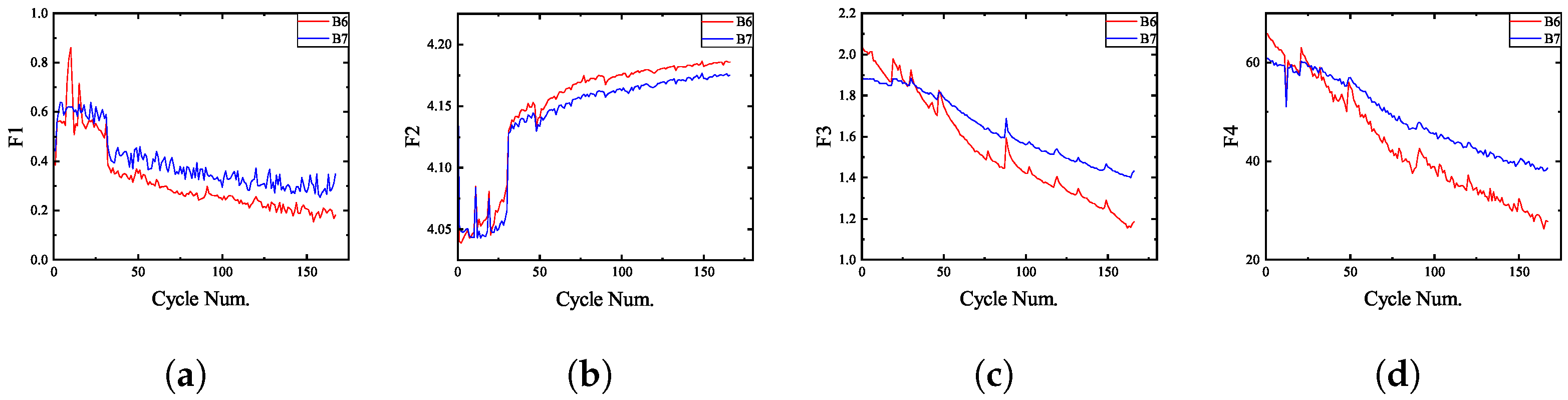
Figure 7.
Four health features extracted from the NASA dataset. (a) F1. (b) F2. (c) F3. (d) F4.

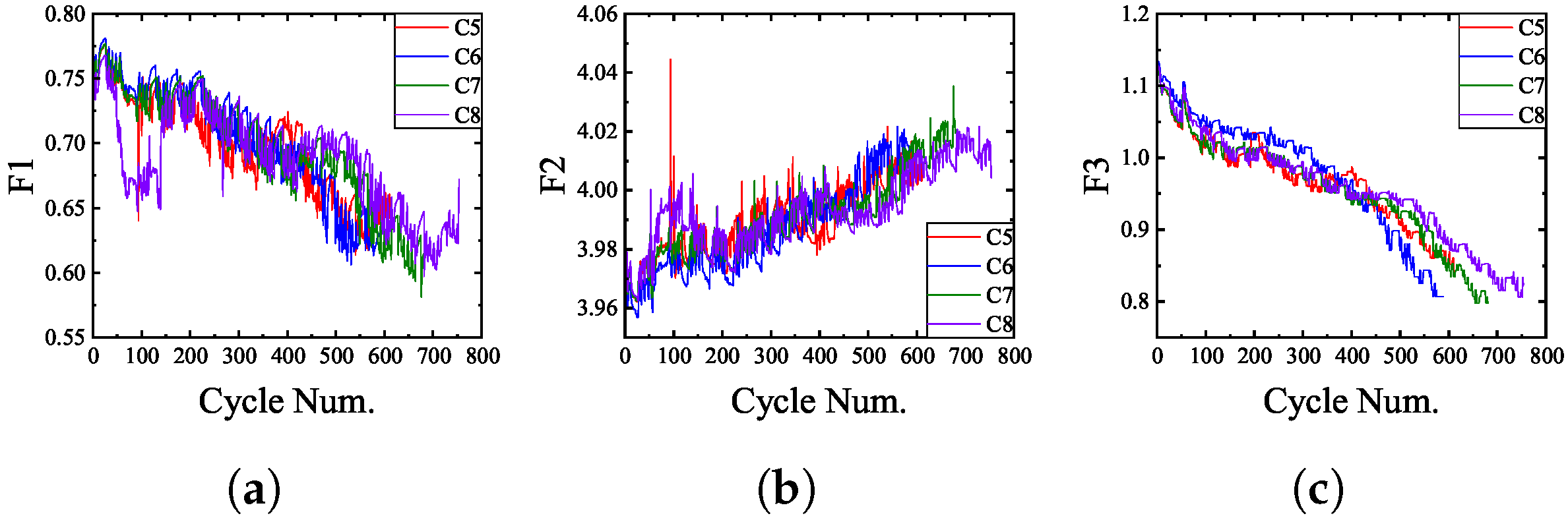
Figure 8.
Three health features extracted from the CALCE dataset. (a) F1. (b) F2. (c) F3.

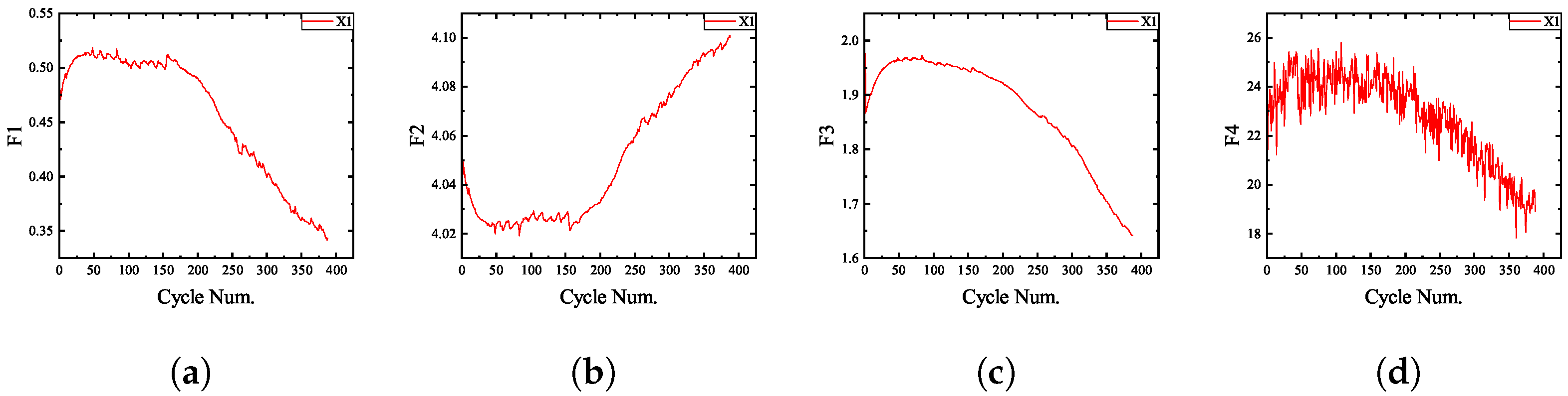
Figure 9.
Four health features extracted from the XJTU dataset. (a) F1. (b) F2. (c) F3. (d) F4.
The NASA batteries exhibit rapid aging, characterized by a decrease in battery capacity (F3) to 80% of the nominal capacity in less than 100 cycles. As these batteries degrade, the proportion of constant current charging time (F1) decreases while the average value of the constant current charging voltage (F2) increases. In contrast, the CALCE batteries demonstrate slower aging, with the battery capacity only declining to 80% of the nominal capacity after at least 600 cycles. The changes in F1 and F2 of the CALCE batteries exhibit a smoother transition throughout the aging cycle, and any anomalous data observed are attributed to experimental interruptions. Both types of batteries display a notable capacity recovery in the early stages of aging, followed by a gradual decline in the amount of capacity recovery in the later stages. The variations in the features of the XJTU batteries exhibit relative stability.
Normalization can enhance predictive accuracy and accelerate training speed, playing a crucial role in many machine learning and data analysis tasks. Adjusting the value range of input features in the dataset to the same scale allows all features to be treated equally during model training. For example, the range of the F1 health feature in this paper is (0, 1), which is significantly different from other features. The min-max normalization method is used to normalize the HFs, speed up the solution, and improve prediction accuracy, as shown in Equation (22).
The root mean squared error (RMSE), mean absolute errors (MAE), and the coefficient of determination () were used to evaluate the estimation results. The definition of RMSE is shown in Equation (21), and the definitions of MAE and are as follows:
The prediction performance of the model is excellent, with RMSE and MAE approaching 0 and approaching 1.
4.3. Analysis of Results
4.3.1. Performance of HHO-LSTM-FC on NASA Datasets
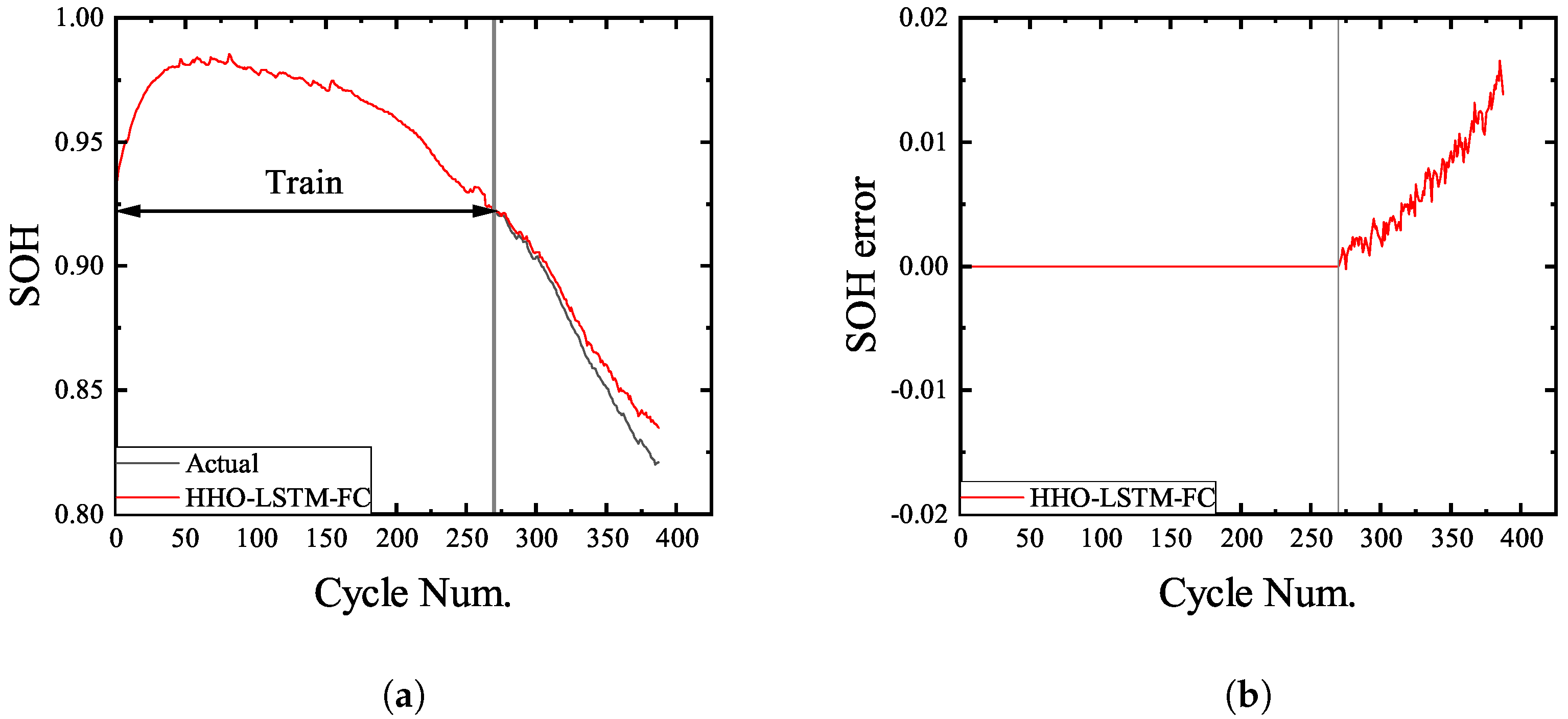
As a time series analysis method, LSTM produces good results for SOH prediction. A fully connected (FC) neuron is connected to every neuron in the previous layer, which allows it to learn global information from the input data rather than just local information. The adaptive moment estimation optimizer (Adam) improves the LSTM-FC model’s performance, which adaptively adjusts the learning rate. The HHO algorithm can find the most suitable parameters for the LSTM-FC model, improving the base model’s performance. This paper selects two sets of battery data, B0006 and B0007, to verify the accuracy and generalization of the proposed model. The first 40% of the data is used as a training set, and the last 60% is used as a test set. Finally, the optimized model structure for the B0006 battery consists of an LSTM layer with 26 neurons and an FC layer with 10 neurons. The optimized model structure for the B0007 battery consists of an LSTM layer with 27 neurons and an FC layer with 10 neurons. The HHO-LSTM-FC prediction results and errors are shown in Figure 10.

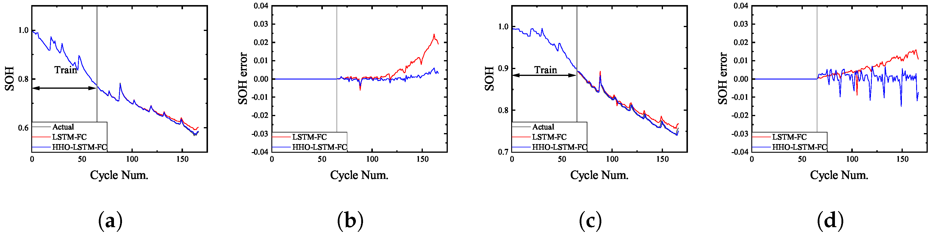
Figure 10.
Comparison of HHO-LSTM-FC and LSTM-FC. (a) Prediction outcomes for B6. (b) Error in prediction outcomes for B6. (c) Prediction outcomes for B7. (d) Error in prediction outcomes for B7.
The predicted SOH curves are always close to actual SOH values. Furthermore, the model optimized using the HHO algorithm exhibits superior prediction performance and has fewer minor errors. Table 2 presents a more comprehensive evaluation result, where the model’s prediction error has been reduced by more than half. Table 3 compares the RMSE results of our model with those of other models for estimating NASA battery health.
Table 2.
SOH estimation errors for NASA cells.
Table 3.
Comparison between the RMSEs obtained for the SOH evaluation of NASA batteries and other methods in the literature.
Table 3 shows that our method has better evaluation accuracy, and our training set data ratio is the smallest (only 40%). When optimized using the HHO algorithm, the model adapts well to the NASA dataset and accurately estimates SOH values.
4.3.2. Performance of HHO-LSTM-FC-TL on CALCE Datasets
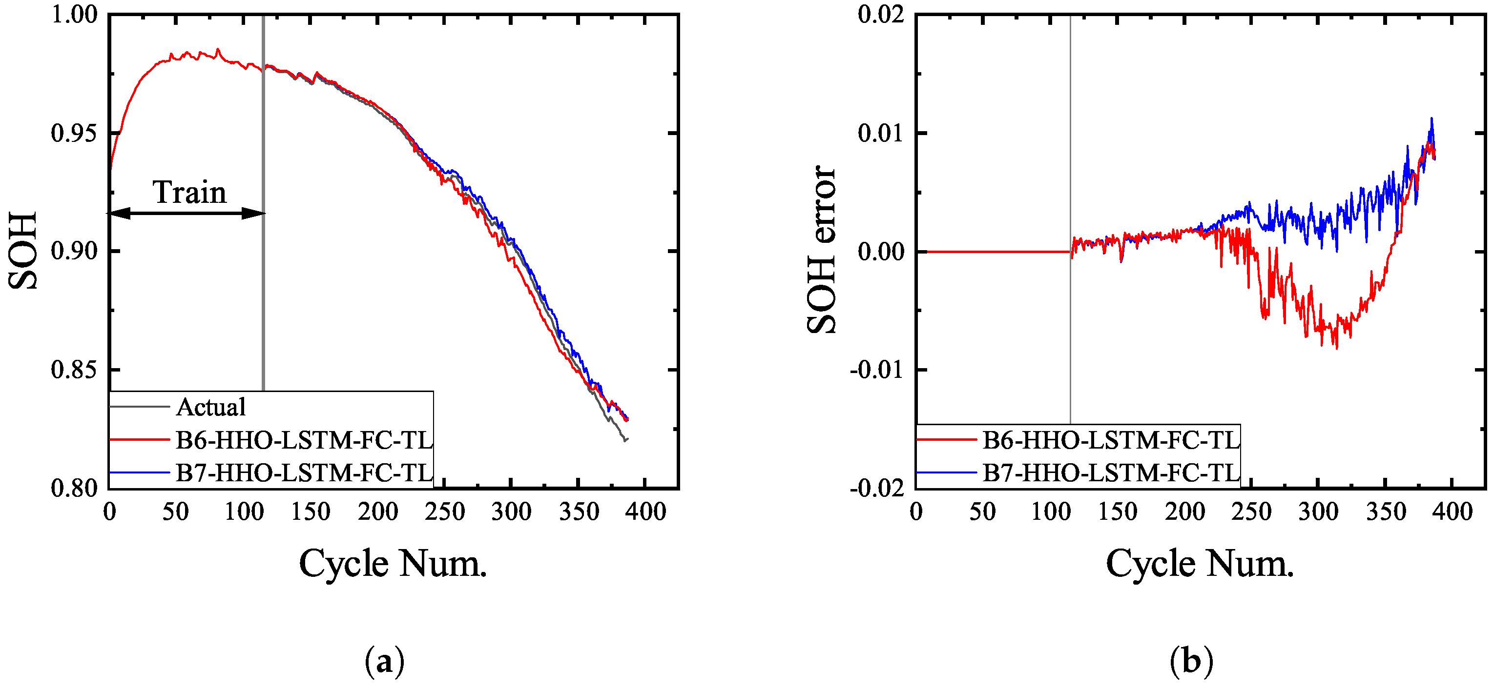
The CALCE dataset was selected to test the proposed method’s performance on different datasets through transfer learning. For the CALCE dataset, a fine-tuning strategy was implemented on the FC layer, and the transfer model takes 30% of the data to train and update the FC layer weights. By using the initial 40% of the B6 and B7 datasets, we trained our base models to demonstrate the effectiveness of the proposed method. Given the lack of temperature data recording in CALCE, only three features—F1, F2, and F3—were employed for training. The results of the transfer models are depicted in Figure 11 and Figure 12. A comparison was made with the HHO-LSTM-FC method, which only uses the first 30% of the CALCE data as a training set. For the case where the B6 battery data were taken as the source domain and the CALCE data as the target domain, the optimized model structure consists of an LSTM hidden layer with 60 neurons and an FC layer with 10 neurons. Correspondingly, for the case where B7 was used as the source domain, the optimized model structure consists of an LSTM hidden layer with 70 neurons and an FC layer with 20 neurons.

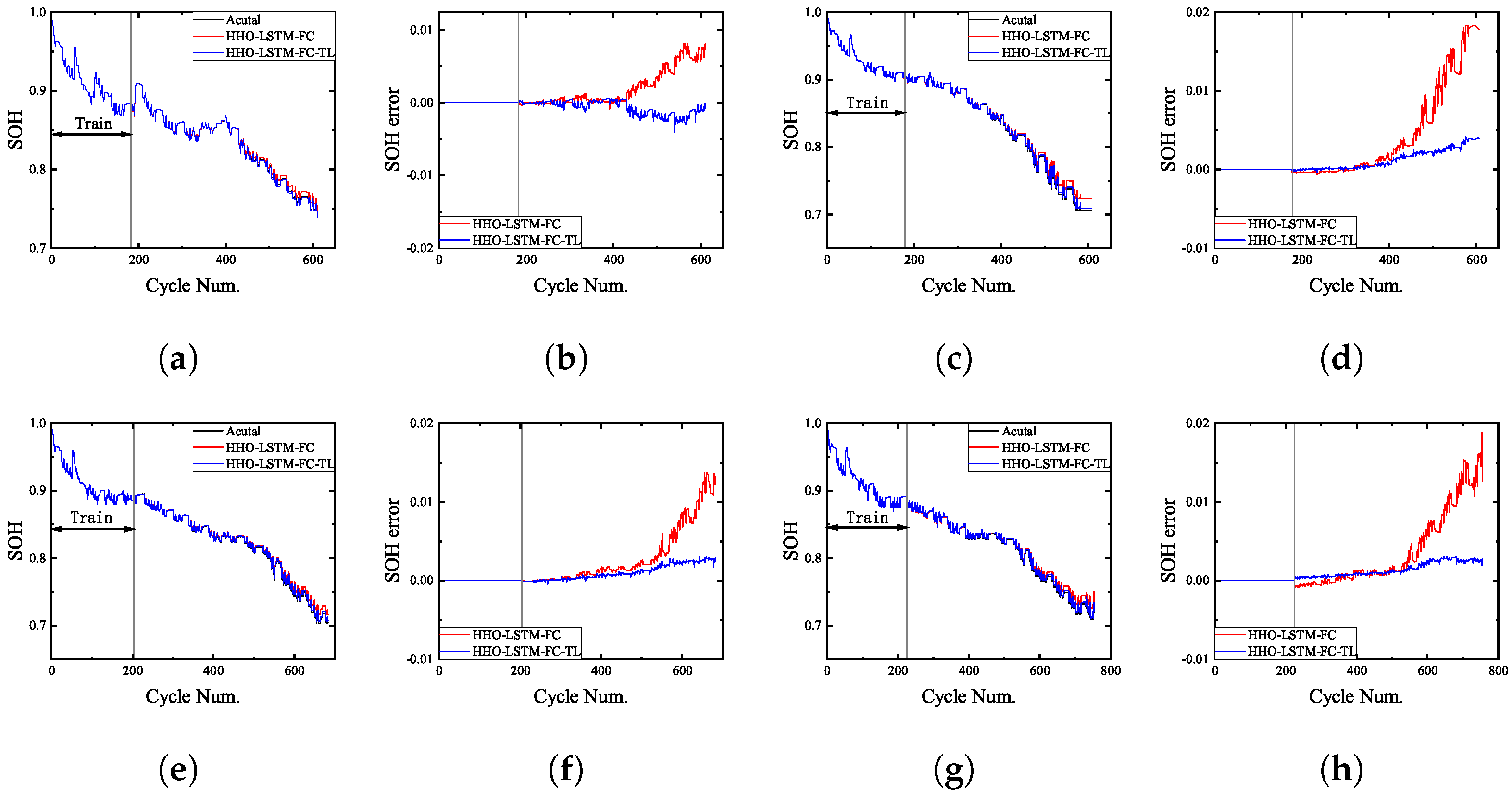
Figure 11.
Performance comparison of HHO-LSTM-FC and HHO-LSTM-FC-TL, migrating the knowledge of B6 for the CALCE dataset. (a) Prediction outcomes for C5. (b) Error in prediction outcomes for C5. (c) Prediction outcomes for C6. (d) Error in prediction outcomes for C6. (e) Prediction outcomes for C7. (f) Error in prediction outcomes for C7. (g) Prediction outcomes for C8. (h) Error in prediction outcomes for C8.

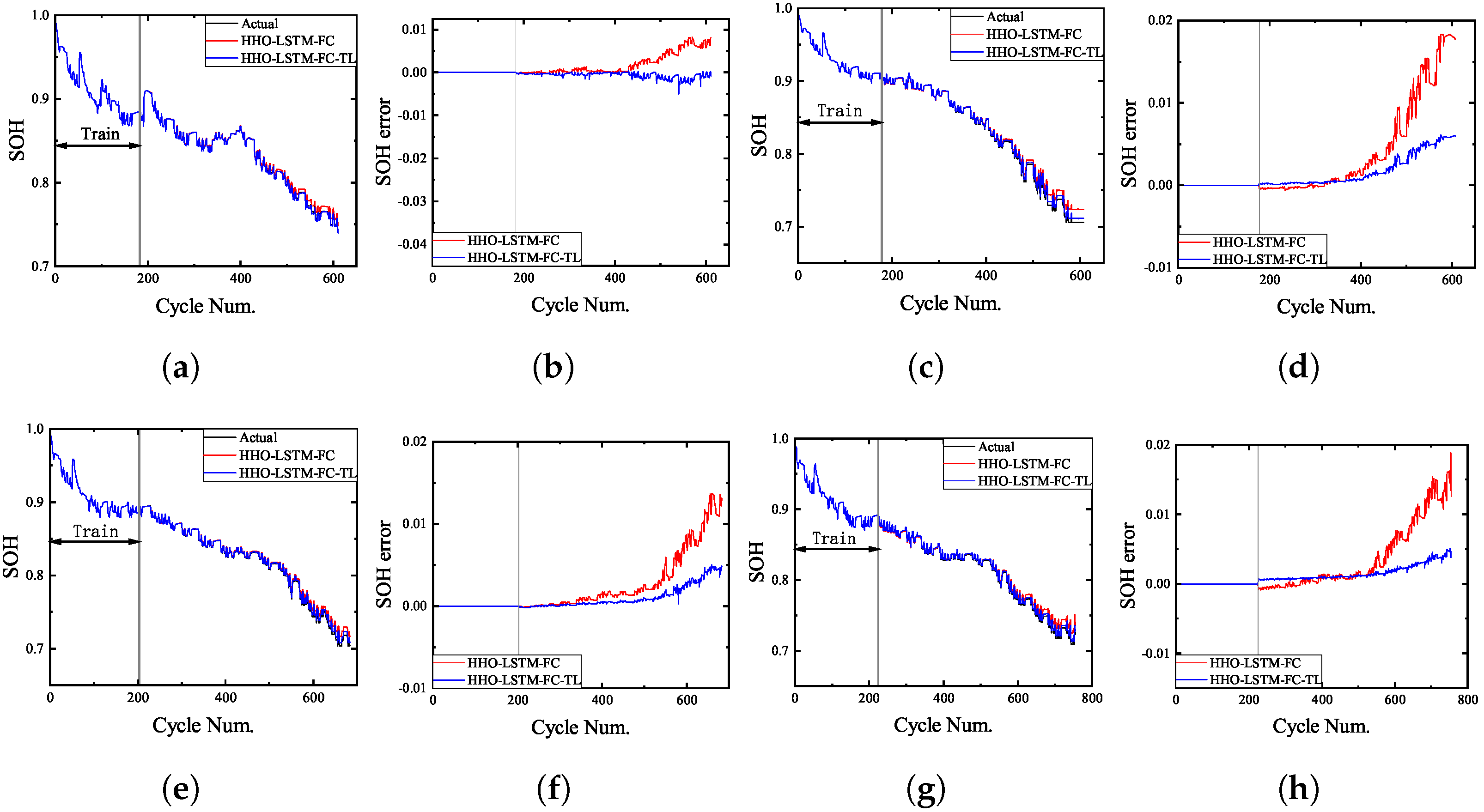
Figure 12.
Performance comparison of HHO-LSTM-FC and HHO-LSTM-FC-TL, migrating the knowledge of B7 for the CALCE dataset. (a) Prediction outcomes for C5. (b) Error in prediction outcomes for C5. (c) Prediction outcomes for C6. (d) Error in prediction outcomes for C6. (e) Prediction outcomes for C7. (f) Error in prediction outcomes for C7. (g) Prediction outcomes for C8. (h) Error in prediction outcomes for C8.
In the latter half of the prediction, the model with transfer learning maintains a high level of accuracy. In contrast, the base model without transfer knowledge experiences a decline in accuracy in the latter 50% of the prediction process. Table 4 shows the numerical comparison indicators of different methods. It can be seen that the proposed transfer model, which learns “knowledge” from the B6 battery, performs slightly better on the CALCE dataset than B7, and both are superior to the HHO-LSTM-FC model.
Table 4.
Performance comparison of different methods for CALCE.
Furthermore, to validate the proposed SOH prediction method’s advanced nature, a comparison with other experiments conducted under the CALCE dataset is shown in Table 5. Our model achieves high accuracy within the battery’s permissible usage range, with an RMSE of less than 0.2%.
Table 5.
Performance of different experiments using the C7 dataset.
4.3.3. Performance of HHO-LSTM-FC-TL on the XJTU Dataset
For the XJTU dataset, the base model was trained using the initial 40% of the B6 and B7 data. The transfer model then employed 30% of the data to train and update the weights of the FC layer, thereby demonstrating the effectiveness of the proposed method. The results are shown in Figure 13. For the case where the B6 battery data were taken as the source domain and the XJTU data as the target domain, the optimized model structure consists of an LSTM hidden layer with 20 neurons and an FC layer with 20 neurons. Correspondingly, for the case where B7 was used as the source domain, the optimized model structure consists of an LSTM hidden layer with 20 neurons and an FC layer with 10 neurons. In contrast, Figure 14 shows that X1 requires 70% of the data for training when the transferred knowledge is not utilized. It is evident that the transferred knowledge has had a significant impact. This knowledge transfer has led to a reduction in the training data required for battery X1, thereby substantially reducing the training cost. Table 6 presents the detailed metrics associated with the transfer model.

Figure 13.
The performance of the HHO-LSTM-FC-TL model transferring knowledge from NASA to the XJTU dataset. (a) Prediction outcomes for X1. (b) Error in prediction outcomes for X1.

Figure 14.
The performance of the HHO-LSTM-FC-TL model on the XJTU dataset. (a) Prediction outcomes for X1. (b) Error in prediction outcomes for X1.
Table 6.
SOH estimation errors for XJTU cells.
5. Conclusions
This study proposes a battery SOH prediction method based on a transferable LSTM-FC network optimized by the HHO algorithm. This study contributes the following main findings. (1) Four aging features— the proportion of constant current charging time, the average value of constant current charging voltage, the charging capacity, and the time to reach maximum temperature—were extracted based solely on the charging phase. Spearman correlation analysis shows a strong correlation with SOH. (2) In order to solve the problem of parameter optimization identification in neural network prediction, we propose a method to optimize the LSTM-FC network and LSTM-FC-TL by using the HHO algorithm. In the estimation of SOH, the RMSE is less than 0.4%, and the MAE is less than 0.3%. (3) Transfer learning was employed in order to achieve accurate and stable predictions of SOH. The transfer model was trained by only using the first 30% of the battery data in the target domain, effectively addressing the problem of limited data for novel tasks, which significantly improved the practicality of the prediction model. The knowledge transferred can effectively improve SOH prediction accuracy in the later stages of battery usage. Combining the HHO algorithm and transfer learning can reduce the time for manual parameter tuning and maximize the model’s performance, which significantly improves the model’s generalization. However, the limitation of this method is that applying the model to batteries with different charging modes may require additional model training and adjustment. By accurately predicting SOH, the method promotes efficient resource utilization and reduces environmental impact, aligning with the goals of sustainable technology adoption. Future research will explore transfer learning methods for lithium batteries with different charging protocols and chemical compositions, thereby enhancing the applicability and sustainability of battery management systems.
Author Contributions
Conceptualization, X.W. and G.Y.; methodology, X.W.; software, X.W.; validation, X.W., G.Y., R.L. and X.Z.; formal analysis, X.W. and G.Y.; investigation, X.W.; writing—original draft preparation, X.W. and G.Y.; writing—review and editing, X.W. and G.Y.; visualization, X.W.; supervision, G.Y., R.L. and X.Z.; project administration, X.W., G.Y. and R.L.; funding acquisition, R.L. All authors have read and agreed to the published version of the manuscript.
Funding
This research was supported in part by the Natural Science Foundation of Heilongjiang Province, China, under Grant LH2022E088, and in part by the Harbin manufacturing science and technology innovation talent project under Grant 2022HBRCCG006.
Institutional Review Board Statement
Not applicable.
Informed Consent Statement
Not applicable.
Data Availability Statement
The data presented in this study are available on request from the corresponding author.
Acknowledgments
The authors would like to thank the NASA Prognostics Center of Excellence, the Centre for Advanced Life Cycle Engineering, and Xi’an Jiao Tong University for providing the experimental data.
Conflicts of Interest
The authors declare no conflict of interest.
References
- Xu, J.; Sun, C.; Ni, Y.; Lyu, C.; Wu, C.; Zhang, H.; Yang, Q.; Feng, F. Fast identification of micro-health parameters for retired batteries based on a simplified P2D model by using padé approximation. Batteries 2023, 9, 64. [Google Scholar] [CrossRef]
- Hu, X.; Xu, L.; Lin, X.; Pecht, M. Battery lifetime prognostics. Joule 2020, 4, 310–346. [Google Scholar] [CrossRef]
- Zhu, J.; Mathews, I.; Ren, D.; Li, W.; Cogswell, D.; Xing, B.; Sedlatschek, T.; Kantareddy, S.N.R.; Yi, M.; Gao, T.; et al. End-of-life or second-life options for retired electric vehicle batteries. Cell Rep. Phys. Sci. 2021, 2, 100537. [Google Scholar] [CrossRef]
- Ruan, H.; Wei, Z.; Shang, W.; Wang, X.; He, H. Artificial Intelligence-based health diagnostic of Lithium-ion battery leveraging transient stage of constant current and constant voltage charging. Appl. Energy 2023, 336, 120751. [Google Scholar] [CrossRef]
- Lin, M.; Yan, C.; Wang, W.; Dong, G.; Meng, J.; Wu, J. A data-driven approach for estimating state-of-health of lithium-ion batteries considering internal resistance. Energy 2023, 277, 127675. [Google Scholar] [CrossRef]
- Zhou, L.; Zhang, Z.; Liu, P.; Zhao, Y.; Cui, D.; Wang, Z. Data-driven battery state-of-health estimation and prediction using IC based features and coupled model. J. Energy Storage 2023, 72, 108413. [Google Scholar] [CrossRef]
- Li, X.; Lyu, M.; Li, K.; Gao, X.; Liu, C.; Zhang, Z. Lithium-ion battery state of health estimation based on multi-source health indicators extraction and sparse Bayesian learning. Energy 2023, 282, 128445. [Google Scholar] [CrossRef]
- Chen, J.; Hu, Y.; Zhu, Q.; Rashid, H.; Li, H. A novel battery health indicator and PSO-LSSVR for LiFePO4 battery SOH estimation during constant current charging. Energy 2023, 282, 128782. [Google Scholar] [CrossRef]
- Zhao, J.; Xuebin, L.; Daiwei, Y.; Jun, Z.; Wenjin, Z. Lithium-ion battery state of health estimation using meta-heuristic optimization and Gaussian process regression. J. Energy Storage 2023, 58, 106319. [Google Scholar] [CrossRef]
- Wu, M.; Zhong, Y.; Wu, J.; Wang, Y.; Wang, L. State of health estimation of the lithium-ion power battery based on the principal component analysis-particle swarm optimization-back propagation neural network. Energy 2023, 283, 129061. [Google Scholar] [CrossRef]
- Zhang, Y.; Wang, Y.; Zhang, C.; Qiao, X.; Ge, Y.; Li, X.; Peng, T.; Nazir, M.S. State-of-health estimation for lithium-ion battery via an evolutionary Stacking ensemble learning paradigm of random vector functional link and active-state-tracking long–short-term memory neural network. Appl. Energy 2024, 356, 122417. [Google Scholar] [CrossRef]
- Li, W.; Sengupta, N.; Dechent, P.; Howey, D.; Annaswamy, A.; Sauer, D.U. Online capacity estimation of lithium-ion batteries with deep long short-term memory networks. J. Power Sources 2021, 482, 228863. [Google Scholar] [CrossRef]
- Tagade, P.; Hariharan, K.S.; Ramachandran, S.; Khandelwal, A.; Naha, A.; Kolake, S.M.; Han, S.H. Deep Gaussian process regression for lithium-ion battery health prognosis and degradation mode diagnosis. J. Power Sources 2020, 445, 227281. [Google Scholar] [CrossRef]
- Wang, Y.; Meng, D.; Wang, Y.; Li, R.; Zhou, Y. Research on health state estimation methods of lithium-ion battery for small sample data. Energy Rep. 2022, 8, 2686–2698. [Google Scholar] [CrossRef]
- Feng, H.; Shi, G. SOH and RUL prediction of Li-ion batteries based on improved Gaussian process regression. J. Power Electron. 2021, 21, 1845–1854. [Google Scholar] [CrossRef]
- Zhang, Y.; Wik, T.; Bergström, J.; Pecht, M.; Zou, C. A machine learning-based framework for online prediction of battery ageing trajectory and lifetime using histogram data. J. Power Sources 2022, 526, 231110. [Google Scholar] [CrossRef]
- Roman, D.; Saxena, S.; Robu, V.; Pecht, M.; Flynn, D. Machine learning pipeline for battery state-of-health estimation. Nat. Mach. Intell. 2021, 3, 447–456. [Google Scholar] [CrossRef]
- Tang, X.; Yang, M.; Shi, L.; Hou, Z.; Xu, S.; Sun, C. Adaptive state-of-health temperature sensitivity characteristics for durability improvement of PEM fuel cells. Chem. Eng. J. 2024, 491, 151951. [Google Scholar] [CrossRef]
- You, G.W.; Park, S.; Oh, D. Diagnosis of electric vehicle batteries using recurrent neural networks. IEEE Trans. Ind. Electron. 2017, 64, 4885–4893. [Google Scholar] [CrossRef]
- Zhang, Y.; Xiong, R.; He, H.; Pecht, M.G. Long short-term memory recurrent neural network for remaining useful life prediction of lithium-ion batteries. IEEE Trans. Veh. Technol. 2018, 67, 5695–5705. [Google Scholar] [CrossRef]
- Qian, C.; Xu, B.; Chang, L.; Sun, B.; Feng, Q.; Yang, D.; Ren, Y.; Wang, Z. Convolutional neural network based capacity estimation using random segments of the charging curves for lithium-ion batteries. Energy 2021, 227, 120333. [Google Scholar] [CrossRef]
- Li, Q.; Li, D.; Zhao, K.; Wang, L.; Wang, K. State of health estimation of lithium-ion battery based on improved ant lion optimization and support vector regression. J. Energy Storage 2022, 50, 104215. [Google Scholar] [CrossRef]
- Zhang, F.; Xing, Z.-X.; Wu, M.-H. State of health estimation for Li-ion battery using characteristic voltage intervals and genetic algorithm optimized back propagation neural network. J. Energy Storage 2023, 57, 106277. [Google Scholar]
- Jafari, S.; Byun, Y.C. Optimizing battery RUL prediction of lithium-ion batteries based on Harris hawk optimization approach using random forest and LightGBM. IEEE Access 2023, 11, 87034–87046. [Google Scholar] [CrossRef]
- Gadekallu, T.R.; Srivastava, G.; Liyanage, M.; Iyapparaja, M.; Chowdhary, C.L.; Koppu, S.; Maddikunta, P.K.R. Hand gesture recognition based on a Harris hawks optimized convolution neural network. Comput. Electr. Eng. 2022, 100, 107836. [Google Scholar] [CrossRef]
- Zhuang, F.; Qi, Z.; Duan, K.; Xi, D.; Zhu, Y.; Zhu, H.; Xiong, H.; He, Q. A comprehensive survey on transfer learning. Proc. IEEE 2020, 109, 43–76. [Google Scholar] [CrossRef]
- Deng, Z.; Lin, X.; Cai, J.; Hu, X. Battery health estimation with degradation pattern recognition and transfer learning. J. Power Sources 2022, 525, 231027. [Google Scholar] [CrossRef]
- Yao, J.; Han, T. Data-driven lithium-ion batteries capacity estimation based on deep transfer learning using partial segment of charging/discharging data. Energy 2023, 271, 127033. [Google Scholar] [CrossRef]
- Che, Y.; Deng, Z.; Lin, X.; Hu, L.; Hu, X. Predictive battery health management with transfer learning and online model correction. IEEE Trans. Veh. Technol. 2021, 70, 1269–1277. [Google Scholar] [CrossRef]
- Mansoor, H.; Rauf, H.; Mubashar, M.; Khalid, M.; Arshad, N. Past vector similarity for short term electrical load forecasting at the individual household level. IEEE Access 2021, 9, 42771–42785. [Google Scholar] [CrossRef]
- Li, X.; Yuan, C.; Li, X.; Wang, Z. State of health estimation for Li-Ion battery using incremental capacity analysis and Gaussian process regression. Energy 2020, 190, 116467. [Google Scholar] [CrossRef]
- Jorge, I.; Mesbahi, T.; Samet, A.; Boné, R. Time series feature extraction for lithium-ion batteries state-of-health prediction. J. Energy Storage 2023, 59, 106436. [Google Scholar] [CrossRef]
- Saha, B.; Goebel, K. Battery Data Set, NASA Ames Research Center, Moffett Field, CA, USA. NASA Ames Research Center. Moffett Field CA USA. 2007. Available online: https://ti.arc.nasa.gov/tech/dash/groups/pcoe/prognostic-data-repository/ (accessed on 10 May 2024).
- He, W.; Williard, N.; Osterman, M.; Pecht, M. Prognostics of lithium-ion batteries based on Dempster—Shafer theory and the Bayesian Monte Carlo method. J. Power Sources 2011, 196, 10314–10321. [Google Scholar] [CrossRef]
- Wang, F.; Zhai, Z.; Zhao, Z.; Di, Y.; Chen, X. Physics-informed neural network for lithium-ion battery degradation stable modeling and prognosis. Nat. Commun. 2024, 15, 4332. [Google Scholar] [CrossRef]
- Liu, J.; Chen, Z. Remaining useful life prediction of lithium-ion batteries based on health indicator and Gaussian process regression model. IEEE Access 2019, 7, 39474–39484. [Google Scholar] [CrossRef]
- Hochreiter, S.; Schmidhuber, J. Long short-term memory. Neural Comput. 1997, 9, 1735–1780. [Google Scholar] [CrossRef] [PubMed]
- Zhang, C.L.; Luo, J.H.; Wei, X.S.; Wu, J. In defense of fully connected layers in visual representation transfer. In Proceedings of the Pacific Rim Conference on Multimedia, Harbin, China, 28–29 September 2017; Springer: Berlin/Heidelberg, Germany, 2017; pp. 807–817. [Google Scholar]
- Heidari, A.A.; Mirjalili, S.; Faris, H.; Aljarah, I.; Mafarja, M.; Chen, H. Harris hawks optimization: Algorithm and applications. Future Gener. Comput. Syst. 2019, 97, 849–872. [Google Scholar] [CrossRef]
- Liu, K.; Peng, Q.; Che, Y.; Zheng, Y.; Li, K.; Teodorescu, R.; Widanage, D.; Barai, A. Transfer learning for battery smarter state estimation and ageing prognostics: Recent progress, challenges, and prospects. Adv. Appl. Energy 2023, 9, 100117. [Google Scholar] [CrossRef]
- Lin, Z.; Cai, Y.; Liu, W.; Bao, C.; Shen, J.; Liao, Q. Estimating the state of health of lithium-ion batteries based on a probability density function. Int. J. Electrochem. Sci. 2023, 18, 100137. [Google Scholar] [CrossRef]
- Zhu, X.; Wang, W.; Zou, G.; Zhou, C.; Zou, H. State of health estimation of lithium-ion battery by removing model redundancy through aging mechanism. J. Energy Storage 2022, 52, 105018. [Google Scholar] [CrossRef]
- Zhou, D.; Wang, B. Battery health prognosis using improved temporal convolutional network modeling. J. Energy Storage 2022, 51, 104480. [Google Scholar] [CrossRef]
- Yang, D.; Zhang, X.; Pan, R.; Wang, Y.; Chen, Z. A novel Gaussian process regression model for state-of-health estimation of lithium-ion battery using charging curve. J. Power Sources 2018, 384, 387–395. [Google Scholar] [CrossRef]
- Song, C.; Lee, S. Accurate RUL Prediction Based on Sliding Window with Sparse Sampling. In Proceedings of the 2021 15th International Conference on Ubiquitous Information Management and Communication (IMCOM), Seoul, Republic of Korea, 4–6 January 2021; IEEE: Piscataway, NJ, USA, 2021; pp. 1–5. [Google Scholar]
- Yayan, U.; Arslan, A.T.; Yucel, H. A novel method for SoH prediction of batteries based on stacked LSTM with quick charge data. Appl. Artif. Intell. 2021, 35, 421–439. [Google Scholar] [CrossRef]
- Tan, Y.; Zhao, G. Transfer learning with long short-term memory network for state-of-health prediction of lithium-ion batteries. IEEE Trans. Ind. Electron. 2019, 67, 8723–8731. [Google Scholar] [CrossRef]
Disclaimer/Publisher’s Note: The statements, opinions and data contained in all publications are solely those of the individual author(s) and contributor(s) and not of MDPI and/or the editor(s). MDPI and/or the editor(s) disclaim responsibility for any injury to people or property resulting from any ideas, methods, instructions or products referred to in the content. |
© 2024 by the authors. Licensee MDPI, Basel, Switzerland. This article is an open access article distributed under the terms and conditions of the Creative Commons Attribution (CC BY) license (https://creativecommons.org/licenses/by/4.0/).