Abstract
The tropospheric production of O3 is complex, depending on nitrogen oxides (NOx = NO + NO2), volatile organic compounds (VOCs), and solar radiation. We present a case study showing that the O3 concentration is higher in a rural area, 14 km downwind from a coastal town in Central Italy, compared with the urban environment. The hypothesis is that the O3 measured inland results from the photochemical processes occuring in air masses originating at the urban site, which is richer in NOx emissions, during their transport inland.To demonstrate this hypothesis, a feed forward neural network (FFNN) is used to model the O3 measured at the rural site, comparing the modeled O3 and the measured O3 in different scenarios, which include both input parameters related to local O3 production by photochemistry and input parameters associated with regional transport of O3 precursors. The simulation results show that the local NOx concentration is not a good input to model the observed O3 (R = 0.17); on the contrary including the wind speed and direction as input of the FFNN model, the modelled O3 is well correlated with that measured O3 (R = 0.82).
1. Introduction
In recent decades, urban air quality has become a central focus of environmental research, policy making, and public health advocacy. Among the myriad of pollutants affecting the urban atmospheres, O3 stands out due to its adverse effects on respiratory health, agricultural productivity, and ecosystem integrity [1,2]. The formation of the tropospheric O3 involves complex processes: the stratosphere–troposphere air masses exchange [3] and photochemical reactions. These reactions involve the oxidation of carbon monoxide (CO), methane (CH4), and volatile organic compounds (VOCs), catalyzed by nitrogen oxides (NOx), which is the sum of nitric oxide (NO) and nitrogen dioxide (NO2), as well as meteorological parameters such as temperature [4]. In urban areas, daily variations in O3 concentration and its precursors are correlated to rush hours (which cause an increase in road traffic emissions) and to the diurnal patterns of solar radiation and other weather factors affecting the efficiency of photochemical reactions. Besides this, O3 and NOx concentrations are also influenced by the planetary boundary layer variations and advective transport processes, which is affected by the dominant wind direction and regional orography [5]. The O3 precursors, such as organo nitrates, can be transported over long distances due to their longer lifetime, becoming possible sources of O3 in a region far from their production sites [6,7]. It is useful to monitor the air quality and meteorological features with more detail in urban area and background countrysides to evaluate the influence of urban emission sources on the surrounding rural environment, where the local emissions of O3 precursors are negligible [8]. In North-Eastern India, the yearly O3 and NOx concentrations have been monitored in three urban sites (Gauhati, Tezpur, and Aizwal), not affected by industrial emissions. It has been found that surface O3 is not entirely due to local production and that during pre-monsoon and winter seasons, the transport of air masses from industrial areas is the cause of the higher pollutions level registered in the three monitoring sites [9]. Studies conducted in the Los Angeles Basin, a region notorious for its smog and air quality challenges, have provided critical insights into these dynamics. Notably, research by [10,11,12] has shed light on the intricate balance of chemical precursors in O3 formation and the pivotal role of temperature in modulating this balance. The Los Angeles Basin serves as an emblematic case study for understanding O3 trends and the efficacy of air quality management strategies. Despite significant reductions in NOx and VOC emissions due to stringent regulatory measures, O3 levels in the basin remain stubbornly high, often exceeding national ambient air quality standards. The decline in NOx observed over the last decade in Los Angeles, which has not been followed by a reduction in O3, has also been observed in several other urban areas worldwide, including the urban area of Pescara, Central Italy—the object of the present study [13]. The persistent O3 exceedances highlight the non-linear relationship between O3 formation and its precursors, underscoring the importance of a nuanced approach to emission control. Furthermore, studies underscore the impact of temperature, with warmer conditions exacerbating O3 formation through enhanced photochemical reactions and increased emissions of temperature-dependent VOCs. In this work, we used a combination of the observations of O3 and NOx, and meteorological parameters in two sites—one in the urban area and the other inland and downwind of the coastal town—and a neural network technique to assess the origin of elevated O3 concentration in the rural area compared with that in the urban site. The complex orography of the area and the emission mix due to domestic and industrial activities and those due to the presence of an international airport in the urban area, make this study interesting for strategies to mitigate O3 pollution and protect public health in a different geographical context.
2. Materials and Methods
2.1. Site and Observations
The dataset used in this study was collected in Central Italy (Abruzzo). This region is characterized by a peculiar orography with mountainous, hilly, and coastal areas. The highest peaks of the Apennines mountain chain are located in this territory: the Gran Sasso massif (2912 m a.s.l.) in the west/north-west (about 60 km from the Adriatic Coast) and the Mount Maiella (2793 m a.s.l.) in the south-west (about 35 km from the Adriatic Coast) (Figure 1).
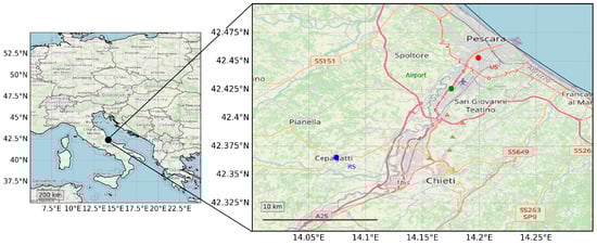
Figure 1.
Map with the location of the monitoring stations employed in this case study. The red is the urban station (US), in the urban area of Pescara (Italy), and the green is the rural downwind station (RS), in a rural area 14 km away from Pescara.
As a consequence, the meteorology of this region is largely affected by the local orography [13]. The coastal area of this area in Central Italy, is characterized by a humid climate with a warm summer and mild winter. Also, the NOx and the O3 annual trends show the expected features with anti correlated trends in summer and winter. Pescara (42.27 N, 14.15 E) is the most populated town along the Adriatic Coast, with about 300.000 inhabitants (from the Italian national statistic institute—ISTAT) in the whole metropolitan area. Moreover, the Abruzzo international Airport and one of the busiest ports of Central Italy are also located in Pescara. Details about the measurement sites, the local meteorological/climatological conditions, and air quality situation can be found elsewhere [13]. Pollutants such as O3 and NOx (NO2 and NO) have been detected simultaneously in the two monitoring stations: Sacco (henceforth, Urban Site (US)) and Cepagatti (henceforth, Rural downwind Site (RS)). The US station is located along the coastline and is in the urban area close to the airport and the main industrial area. On the contrary, the second station (RS) is installed in a rural background site about 14 km from the urban area in the Pescara River Valley (Figure 1).
The data were collected in 2018, with a sampling frequency of 1 h. The whole dataset was used to compare the O3 measured at RS in different meteorological conditions, i.e., for air masses from different wind directions. Due to gaps in the dataset when running FFNN, we selected the period between the end of April and the beginning of July, corresponding to the interval during which the simultaneous availability of the different parameters used as FFNN input was maximized.
2.2. Data Analysis
Figure 2 shows the time series of NO, NO2, NOx, and O3, and the meteorological parameters recorded in May–June 2018 in both the rural and urban monitoring stations, in Figure 2A and Figure 2B respectively.

Figure 2.
Time series of O3, its precursors, and the relevant meteorological parameters from the monitoring station in the urban area (A) and downwind in the rural environment (B).
As depicted, NOx had higher concentrations in the urban station compared with the rural site; on average, it was 22.0 ± 11.9 µg/m3 in the urban environment, whereas it was 7.4 ± 3.3 µg/m3 in the rural area. This significant difference between the urban and rural environments also applies to the maximum values of NOx, which were more than twice as high in the urban site compared with the rural one, as well as for NO and NO2, see Table 1 for a detailed comparison between the two environments. Interestingly, the mean O3 concentration was higher in the inland rural station, at about 34 µg/m3 (Table 1), suggesting the possibility of O3 production in rural areas due to photochemical processes during the transport of air masses from the urban coastal sites to the background station by regional transport.

Table 1.
Basilar statistics of NO, NO2, NOx, and O3 measured between 1 May and 29 June 2018 at the urban monitoring station (US) and at the rural downwind station (RS).
2.3. Model Analysis
A feed-forward neural network (FFNN) was adopted to accurately predict the O3 concentrations at the RS site, diverging from the recurrent neural network (RNN) models that are traditionally prevalent in this field [13,14]. This strategic choice was influenced by our specific prediction objectives and the rich, multidimensional dataset, rather than by the temporal nature of the data. FFNN networks are renowned for their capacity to discern complex patterns within a diverse array of data, a feature that proves useful in our context, where the aim is to integrate chemical and meteorological inputs from a range of monitoring stations [15,16,17]. The architecture of FFNN networks, with their unidirectional data flow from input to output, is exceptionally effective at identifying intricate, static patterns in data. Our FFNN model is specifically tailored to process variables such as nitrogen oxides (NOx, NO2, and NO) and various meteorological factors from the RS and US stations, to model the O3 levels at the RS location. The predictive model was implemented in Python 3.10, utilizing the TensorFlow Keras library (https://www.tensorflow.org ver. 2.16) for its extensive deep learning functionalities [18]. The input neurons, as depicted in Figure 3, included NO, NO2, NOx, wind speed (WS), wind direction (WD) relative humidity (RH), and temperature (T) measured at the rural site. The model performance was critically evaluated using statistical metrics, including Pearson’s linear correlation index (R), Root Mean Squared Error (RMSE), and Mean Absolute Percentage Error (MAPE).
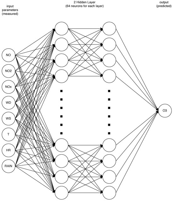
Figure 3.
Schematic illustration of the FF networks employed in this study.
Pearson’s R measures the linear association between the predicted and observed O3 values, while RMSE quantifies the model’s prediction errors. MAPE offers insight into the model accuracy by expressing forecast errors as a percentage of the actual values. These metrics collectively guide the iterative refinement of the model to ensure the most accurate O3 concentration predictions.
The validation process of the FFNN model involved splitting the dataset into training and testing subsets, ensuring that the model performance could be evaluated on unseen data. The training set was used to train the model, while the testing set was used to evaluate its predictive capability. The data were also standardized to improve the model performance. For each scenario, the model was trained and tested multiple times, and the best-performing model was selected based on the highest Pearson correlation coefficient. The scenario with the best performance included input parameters such as nitrogen oxides (NO, NO2, NOx), wind speed, wind direction, relative humidity, and temperature, achieving a high correlation coefficient (R) of 0.90. This indicates that the model performed exceptionally well in capturing the relationship between these variables and the O3 levels. The model’s performance was also evaluated using external datasets by testing on data that were not part of the training set, ensuring that the model’s predictions were generalizable and reliable across different data samples. This comprehensive approach to validation demonstrated that the model could accurately predict O3 concentrations in various scenarios, reinforcing its robustness and applicability in real-world settings.
Quality check and preprocessing of the dataset is crucial to provide accurate and reliable inputs to the FFNN model. As a first step, the missing or inconsistent data have been removed for the whole dataset, imputing missing values using statistical methods like mean or median where necessary. The outliers were identified using statistical techniques, such as standard deviation, and then either corrected or removed based on the domain knowledge. Finally, for temporal data, we ensured the alignment of time series data from different sources, verifying that those observations corresponded correctly over time.
3. Results and Discussion
The local O3 concentration was due to two main mechanisms that determined it: The local photochemistry and the regional transport. We investigated the O3 production mechanism in a rural background site, considering both the local photochemistry and the regional transport from a metropolitan area, where the urban station is installed (Table 1 and Figure 1). In order to evaluate the relationship between O3 and NO2 and NO, we compared the diurnal trends of these compounds and NOx in both stations (Figure 4C).
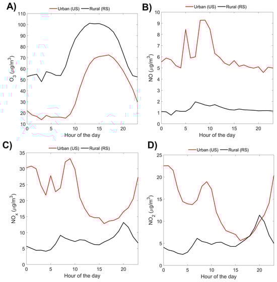
Figure 4.
Diurnal trend. O3 (A), NO (B), NOx (C), and NO2 (D) measured at the urban station (US) and at the rural downwind site (RS).
Even if the mutual interactions in the troposphere between O3, NO2, and NO are complex and other chemical and deposition processes should be considered, from Figure 4A, we can identify that, remarkably, in the rural background station, the concentration of O3 is, on average, higher than the O3 levels detected in the urban station. This can be explained as follows: Considering that the regional transport could move air masses, richer in O3 and its precursors (i.e., NOx), from the densely populated coastal area (US) to the inland hilly areas (RS). The relatively high NO concentration, measured even during the night at the US station (Figure 4B), explains the lower O3 measured in this site (Figure 4A) that, by reacting with NO, produces nocturnal NO2 (Figure 4D). The higher NO concentration in the US can be explained by considering the position of this station, which is installed in a heavy traffic and industrial area of the town. On the other hand, at the background RS station, the NO (Figure 4B) shows a low concentration with a small peak at around 08:00 a.m., corresponding to the morning rush hour. The NOx is about five times lower than those measured in the US station, with a typical diurnal trend with the daytime and late afternoon peaks related to vehicle traffic emissions (Figure 4C). Because of the low NO concentration in RS, the O3 titration between midnight and 7 AM is significantly less efficient in RS than in US, and the O3 concentration in this interval is about double than those sampled in US. At the same time, the local NO2 and NO at RS is too low to explain the local O3 level, suggesting that its origin should be due to its precursors transport from the US area to the background site (RS). These findings are confirmed by analysing the wind speed measured in the US and RS stations and the relationship between the O3 measured at the rural downwind site and the wind direction (Figure 5).
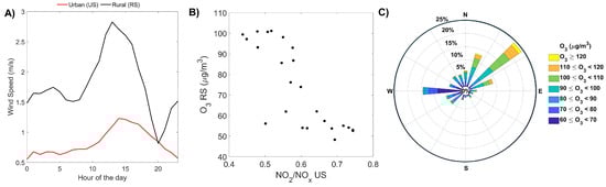
Figure 5.
Diurnal trend of the wind speed (A) measured at the urban station (US) and rural downwind station (RS). O3 measured at RS as a function of the NO2/NOx ratio measured at the US (B). Wind rose of the O3 measured at the RS (C).
Because of the wind speed of the air masses reported at the US (Figure 5A), it is possible to estimate that the NOx produced in the US station by traffic and industrial emissions travelled for about 3 to 7 h to reach the rural station. Despite the chemistry of NOx and O3 being complex, the quick NO conversion to NO2 and the resulting O3 production is a well-known mechanism for explaining O3 production during the transport process of its precursors, i.e., NO2, which can cause a higher concentration of O3 in the rural region, e.g., lacking local sources of O3 precursors, downwind of an urban/industrial area. The time to transport air masses from the US to RS is in line with the NOx lifetime expected in the troposphere. Figure 5B) shows the relation between the O3 measured at the RS station and the NO2 to NOx ratio measured at the urban area, where the main emissions of O3 precursors could trigger the high O3 concentration sampled in the rural site with very low local emission of NO. As expected, when the NO2/NOx ratio is low in the US, meaning that the NO emission is more significant (as also shown in Figure 4B,D), the O3 in the RS is higher, confirming the possible mechanism of O3 production at RS from NO–NO2 photochemistry during the air masses transport from US to RS. Figure 5C shows the polar plot of the O3 measured at the RS station. The highest values of O3 occurs when the winds blow from North-East, i.e., from the urban site with higher NOx. On the contrary, with winds coming from West (inland mountains), the O3 concentration is much lower, confirming that in inland regions, the origin of O3 is not related to local emissions, but due to transport from coastal areas with higher concentrations of NOx and O3. Figure 6 shows an intercomparison between the O3 measured at the RS during the period investigated in this case study and the O3 measured at the same site during the 2018 selecting only air masses from the West, i.e., from the hill and mountainous areas of this region characterized by cleaner air. It is evident from Figure 6 that the O3 at the RS is strongly affected by the origin of the air masses and, in detail, by the NO and NO2 emitted at the US, which is located east of the RS site.
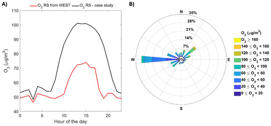
Figure 6.
Comparison between O3 measured (A) at the RS when the wind is blowing from the west (clean air) (B) and the O3 measured at the RS during the period of this study, i.e., with wind mainly blowing from the east (downwind of the US).
To confirm these results, an FF neural network was employed to identify the mechanisms based on the high O3 level measured at the rural downwind site. Different scenarios were simulated (Table 2) in order to identify whether the O3 concentration measured at the rural site was more important than the local chemistry, i.e., the local emission of NO and NO2, or the O3 production during the regional transport from the urban site where the O3 precursor concentration, i.e., NO and NO2, was significantly higher than the one measured at the RS. The O3 at the rural site was modeled using different parameters as the FFNN model inputs, depending on the simulation scenarios (Table 2).
Table 2.
Results of the several FFNN model scenarios run to predict the O3 measured at the rural site (RS). The input parameters used in the different scenarios have been listed, as well as the main statistical parameters to determine the goodness of the model results. Finally, the slope of the scatter plot between the measured and modelled O3 is also reported.
The selection of specific parameters for each scenario in Table 2 was guided by a scientific understanding of the mechanism behind the high O3 concentration in the RS compared with the one measured at the US. In order to have a reference for the model performance, we included all of the parameters available to simulate the O3 (Scenario 1). To exclude the local production of O3 due to temperature and RH, strictly related to solar radiation, we ran the model including only the chemical compounds and the wind speed and direction (Scenario 2). To exclude the local production of O3 due to the local NO and NO2 emissions, we ran an FFNN including only these measurements (Scenario 3). Finally, to prove our hypothesis that the O3 at the RS was the result of the transport of NO and NO2 from the metropolitan area, we ran the FFNN model only considering the wind speed and direction as the inputs (Scenario 4). All of the statistical parameters for determining the goodness of the model results between Scenario 2 and Scenario 4 were similar, demonstrating that the O3 at the RS can be explained mainly by its precursors transport from the US.
As expected, the best simulation is the one corresponding to the first scenario (Figure 7), in which NOx, NO, NO2, WS, WD, T, and HR were used as the inputs for the FFNN model (R = 0.90).
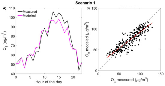
Figure 7.
Model results for Scenario 1. Diurnal mean of the measured and modelled O3 at the rural site (RS) station (A). Scatter plot between the modelled and measured O3 (B). The R is 0.90 and the linear fitting slope is 0.77 (red line). The back line is the 1:1 line.
Furthermore, to understand the causes behind the higher O3 measured at the rural site, it is interesting to observe that, when only the NO, NO2, and NOx (Scenario 3) measured at Rthe S are used as the inputs, the FFNN model is not able to reproduce the O3 both in term of absolute value and diurnal trend (Figure 8), with a correlation coefficient of R = 0.17.
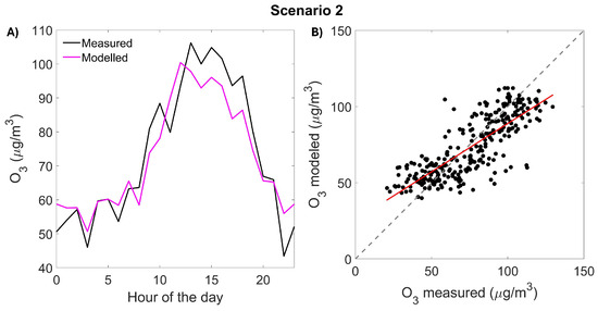
Figure 8.
Similar to Figure 7, but for Scenario 2. Diurnal mean of the measured and modelled O3 at the rural site (RS) station (A). Scatter plot between the modelled and measured O3 (B).The R is 0.81 and the linear fitting slope is 0.63 (red line). The back line is the 1:1 line.
On the other hand, if these inputs also included the wind speed and direction (Scenario 2), the correlation coefficient significantly increased, reaching 0.81 (Figure 9).
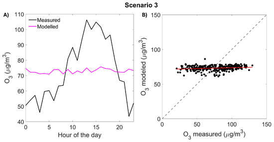
Figure 9.
Similar to Figure 7, but for Scenario 3. Diurnal mean of the measured and modelled O3 at the rural site (RS) station (A). Scatter plot between the modelled and measured O3 (B).The R is 0.17 and the linear fitting slope is 0.02 (red line). The back line is the 1:1 line.
This result strongly suggests that wind speed and direction are the most relevant inputs to model the observed O3. It should be observed that in this scenario, despite the temperature, a well-known proxy to model O3, was not included as an input parameter, the correlation coefficient between the model and measured O3 at the RS station was very high and comparable to the one obtained for the first scenario. This suggests that transport is a possible explanation for the higher concentration of O3 inland compared with the one measured in the urban area. Finally, the FFNN was run using only the wind speed and direction as the input (Scenario 4, Figure 10); the correlation coefficient between the measured and modelled O3 was about 0.81, close to the one obtained when including NO, NO2, and NOx (Scenario 3).
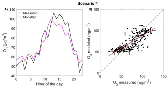
Figure 10.
Similar to Figure 7, but for Scenario 4. Diurnal mean of the measured and modelled O3 at the rural site (RS) station (A). Scatter plot between the modelled and measured O3 (B).The R is 0.81 and the linear fitting slope is 0.60 (red line). The back line is the 1:1 line.
This confirms that the high O3 level measured at the rural downwind site was not related to the local production of O3 precursor species (NO and NO2) and their local photochemistry, but it was mainly due to the photochemical processes that took place in the air masses emitted at the urban site during the downwind transport. It is interesting to observe that the model underestimated the measurements especially between 12:00 and 17:00 p.m., i.e., at the maximum O3 concentration. This could be related to some missing chemical compounds relevant to O3 formation, such as volatile organic compound (VOC) oxidation products or organo nitrates (i.e., peroxy acetyl nitrate (PAN)) that could be dissociated back into NO2, which were not included in the model as they had not been measured.
4. Conclusions
Higher O3 concentrations weremeasured at an inland rural site and were compared with the nearest coastal urban site in Central Italy. We found that the NOx directly emitted in the urban environment during transport resulted in higher levels of O3 produded about 14 km downwind from the NOx source areas. An FFNN model was employed to identify the mechanism to explain O3 production in the rural environment. It was found that the local NOx, which was significantly lower than the one measured in urban area, was totally irrelevant for modelling the local O3 at the rural downwind station (RS). On the other hand, including the wind speed and direction as the input for the model, which were proxies of the regional transport, the correlation between the measured and modelled O3 in the rural site increased significantly (from R = 0.07 using only NO, NO2, and NOx to R = 0.82 by also adding the wind speed and direction). These results are another piece of evidence that the surface O3 formation is rather complicated especially in complex orography where the area downwind of an urban coastal area can be strongly affected by emissions from far away with implications on policy to control and mitigate air quality. The two main limitations of this analysis were the length of the analyzed dataset, which only focused on 2018, and the absence of VOC measurements in both the rural and urban monitoring stations. As a consequence, our work will need further research and field campaigns to analyse the impact of VOCs and organo nitrates to fully explain the mechanisms behind the O3 chemistry in this complex mountain–hill–coast region.
Author Contributions
P.C. had the following roles: conceptualization, data curation, formal analysis, methodology, software, writing—original draft, review, and editing. E.A. had the following roles: conceptualization, formal analysis, investigation, writing—original draft, review, and editing. A.M. contributed to writing—original draft, review, and editing. C.C., S.P. and S.B. contributed to the data curation and writing—review and editing. P.D.C. contributed to the conceptualization, funding acquisition, supervision, and writing—review and editing. All authors have read and agreed to the published version of the manuscript.
Funding
This work has been funded by the European Union—NextGenerationEU under the Italian Ministry of University and Research (MUR) National Innovation Ecosystem grant ECS00000041 VITALITY–CUP: D73C22000840006.
Institutional Review Board Statement
Not applicable.
Informed Consent Statement
Not applicable.
Data Availability Statement
The data presented in this study are available on request from the corresponding author.
Conflicts of Interest
The authors declare no competing financial interests and no competing non-financial interests.
References
- Avnery, S.; Mauzerall, D.L.; Liu, J.; Horowitz, L.W. Global crop yield reductions due to surface ozone exposure: 1. Year 2000 crop production losses and economic damage. Atmos. Environ. 2011, 45, 2284–2296. [Google Scholar] [CrossRef]
- Wang, Y.; Wild, O.; Chen, X.; Wu, Q.; Gao, M.; Chen, H.; Qi, Y.; Wang, Z. Health impacts of long-term ozone exposure in China over 2013–2017. Environ. Int. 2020, 144, 106030. [Google Scholar] [CrossRef] [PubMed]
- Lelieveld, J.; Dentener, F.J. What controls tropospheric ozone? J. Geophys. Res. Atmos. 2000, 105, 3531–3551. [Google Scholar] [CrossRef]
- Pusede, S.E.; Steiner, A.L.; Cohen, R.C. Temperature and Recent Trends in the Chemistry of Continental Surface Ozone. Chem. Rev. 2015, 115, 3898–3918. [Google Scholar] [CrossRef] [PubMed]
- Lei, Y.; Wu, K.; Zhang, X.; Kang, P.; Du, Y.; Yang, F.; Fan, J.; Hou, J. Role of meteorology-driven regional transport on O3 pollution over the Chengdu Plain, southwestern China. Atmos. Res. 2023, 285, 106619. [Google Scholar] [CrossRef]
- Brankov, E.; Henry, R.F.; Civerolo, K.L.; Hao, W.; Rao, S.; Misra, P.; Bloxam, R.; Reid, N. Assessing the effects of transboundary ozone pollution between Ontario, Canada and New York, USA. Environ. Pollut. 2003, 123, 403–411. [Google Scholar] [CrossRef] [PubMed]
- Castell-Balaguer, N.; Téllez, L.; Mantilla, E. Daily, seasonal and monthly variations in ozone levels recorded at the Turia river basin in Valencia (Eastern Spain). Environ. Sci. Pollut. Res. 2012, 19, 3461–3480. [Google Scholar] [CrossRef] [PubMed]
- Agudelo–Castaneda, D.M.; Teixeira, E.C.; Pereira, F.N. Time–series analysis of surface ozone and nitrogen oxides concentrations in an urban area at Brazil. Atmos. Pollut. Res. 2014, 5, 411–420. [Google Scholar] [CrossRef]
- Tyagi, B.; Singh, J.; Beig, G. Seasonal progression of surface ozone and NOx concentrations over three tropical stations in North-East India. Environ. Pollut. 2020, 258, 113662. [Google Scholar] [CrossRef] [PubMed]
- Griffin, R.J.; Revelle, M.K.; Dabdub, D. Modeling the Oxidative Capacity of the Atmosphere of the South Coast Air Basin of California. 1. Ozone Formation Metrics. Environ. Sci. Technol. 2004, 38, 746–752. [Google Scholar] [CrossRef] [PubMed]
- Nussbaumer, C.M.; Cohen, R.C. The Role of Temperature and NOx in Ozone Trends in the Los Angeles Basin. Environ. Sci. Technol. 2020, 54, 15652–15659. [Google Scholar] [CrossRef] [PubMed]
- VanCuren, R. Transport aloft drives peak ozone in the Mojave Desert. Atmos. Environ. 2015, 109, 331–341. [Google Scholar] [CrossRef]
- Biancofiore, F.; Verdecchia, M.; Carlo, P.D.; Tomassetti, B.; Aruffo, E.; Busilacchio, M.; Bianco, S.; Tommaso, S.D.; Colangeli, C. Analysis of surface ozone using a recurrent neural network. Sci. Total Environ. 2015, 514, 379–387. [Google Scholar] [CrossRef] [PubMed]
- Zaini, N.; Ean, L.W.; Ahmed, A.N.; Malek, M.A. A systematic literature review of deep learning neural network for time series air quality forecasting. Environ. Sci. Pollut. Res. 2022, 29, 4958–4990. [Google Scholar] [CrossRef] [PubMed]
- Aruffo, E.; Carlo, P.D.; Cristofanelli, P.; Bonasoni, P. Neural Network Model Analysis for Investigation of NO Origin in a High Mountain Site. Atmosphere 2020, 11, 173. [Google Scholar] [CrossRef]
- Cabaneros, S.M.; Calautit, J.K.; Hughes, B.R. A review of artificial neural network models for ambient air pollution prediction. Environ. Model. Softw. 2019, 119, 285–304. [Google Scholar] [CrossRef]
- Jumin, E.; Zaini, N.; Ahmed, A.N.; Abdullah, S.; Ismail, M.; Sherif, M.; Sefelnasr, A.; El-Shafie, A. Machine learning versus linear regression modelling approach for accurate ozone concentrations prediction. Eng. Appl. Comput. Fluid Mech. 2020, 14, 713–725. [Google Scholar] [CrossRef]
- Vasilev, I.; Slater, D.; Spacagna, G.; Roelants, P.; Zocca, V. Python Deep Learning, Exploring Deep Learning Techniques and Neural Network Architectures with PyTorch, Keras, and TensorFlow; Packt Pub.: Birmingham, UK, 2019. [Google Scholar]


Disclaimer/Publisher’s Note: The statements, opinions and data contained in all publications are solely those of the individual author(s) and contributor(s) and not of MDPI and/or the editor(s). MDPI and/or the editor(s) disclaim responsibility for any injury to people or property resulting from any ideas, methods, instructions or products referred to in the content. |
© 2024 by the authors. Licensee MDPI, Basel, Switzerland. This article is an open access article distributed under the terms and conditions of the Creative Commons Attribution (CC BY) license (https://creativecommons.org/licenses/by/4.0/).