Optimization of Life Cycle Cost and Environmental Impact Functions of NiZn Batteries by Using Multi-Objective Particle Swarm Optimization (MOPSO)

Abstract

This study aims to optimize the Environmental Life Cycle Assessment (LCA) and Life Cycle Cost (LCC) of NiZn batteries using Pareto Optimization (PO) and Multi-objective Particle Swarm Optimization (MOPSO), which combine Pareto optimization and genetic algorithms (GA). The optimization focuses on the raw material acquisition phase and the end-of-life phase of NiZn batteries to improve their sustainability Key Performance Indicators (KPIs). The optimization methodology, programmed in MATLAB, is based on a formulation model of LCC and the environmental LCA, using data available from the Ecoinvent database, the OpenLCA software (V1.11.0), and other public databases. Results provide insights about the best combination of countries for acquiring raw materials to manufacture NiZn and for disposing of the waste of NiZn batteries that cannot be recycled. These results were automatically linked to some sustainability KPIs, such as global warming and capital costs, being replicable in case of data updates or changes in production or recycling locations, which were initially considered at Paris (France) and Krefeld (Germany), respectively. These results provided by an AI model were validated by using a sensitivity analysis and the Analytical Hierarchy Process (AHP) through an expert panel. The sensitivity analysis ensures the robustness of mathematical parameters and future variations in the market; on the other hand, the AHP validates the Artificial Intelligence (AI) results with interactions of human factors. Further developments should also consider the manufacturing and use phases in the optimization model.

1. Introduction

The purpose of this study is to enhance the sustainability of NiZn batteries by optimizing their Environmental Life Cycle Assessment (LCA) and Life Cycle Cost (LCC) through the implementation of Pareto Optimization (PO) and the Multi-objective Particle Swarm Optimization (MOPSO) algorithm. These optimization techniques combine Pareto optimization and genetic algorithms (GA) to improve certain Key Performance Indicators (KPIs).

The evaluation of the environmental impact of consumer goods began in the 1960s and 1970s, but it was between 1970 and 1990 that the LCA was conceived with differing approaches, terminology, and results [1]. The 1990s saw a significant increase in scientific and coordination activities worldwide, resulting in the organization of workshops and forums by SETAC (Society for Environmental Toxicology and Chemistry) and the production of numerous LCA guides and handbooks [2,3]. The International Organization for Standardization (ISO) has also been involved in the LCA since 1994 [4].

The first ISO standard for LCA methodology was published in 1997 [5]. Two years later, Azapagic and Clift, in 1999, proposed a methodology of multi-objective optimization (MOO) coupled with the LCA [6]. This methodology provides a powerful tool for balancing environmental and economic performance, which enables choosing the best practicable environmental option and the best available technique without excessive cost. The methodology was applied to mining and mineral processing operations, specifically for producing several boron products from two mineral ores.

An extensive literature review was conducted to identify an evolutionary algorithm based on the multi-objective optimization method. Finally, the MOPSO algorithm was used to determine the optimum solution.

2. Literature Review and State of the Art

There is currently a lack of research on how to optimize the LCA and life cycle cost analysis (LCCA) using various AI algorithms for batteries and energy storage devices. However, some studies have been conducted on creating algorithms to calculate costs and environmental impact in other fields, such as mining and construction. These algorithms can optimize to determine the most appropriate variable values to minimize both production and operations costs, as well as environmental impact throughout the life of the unit. To gather information for the development of these formulas and optimization of variables, data have been gathered from Google Scholar and ScienceDirect. According to statistics, 42.1% of publications related to multi-objective optimization are in the fields of engineering, material science, environmental sciences, and energy [7].

The first methodology for the integration of the LCA and the economic analysis tool, Life Cycle Costing (LCC), was proposed by Deng et al., 2008 to obtain the integrated evaluation results [8]. In this framework of integration, a mathematical model for environmental and economic subsystems was created, and Multidisciplinary Design Optimization (MDO) was applied to optimize these models so that the initial product design could achieve the best environmental and economic performance. Another study from the year 2015 by Bin Yu et al. [9] in which they developed a multi-objective optimization model that combined four sub-models to integrate pavement performance, cost, and environmental factors. The first sub-model assessed maintenance strategy effectiveness, the second calculated life cycle maintenance costs, and the third compiled life cycle inventories (LCIs) for various activities using the LCA. The fourth sub-model integrated and evaluated these via an optimization algorithm. A simulation–optimization approach combining process simulation, multi-objective optimization, and life cycle assessment was suggested to minimize the LCA impact of thermodynamic cycles and identify optimal design and operating conditions [10]. The utilization of multi-period scenarios in combined LCA and LCCA optimization frameworks and the trend toward the development of generic theoretical LCA frameworks with optimization methodologies were emphasized by Carla Pieragostini et al. in 2011 [11]. However, this study does not provide a specific conclusion on the effectiveness of integrating life cycle cost and the LCA into optimization. Bin Yu et al. implemented their idea and provided a useful methodology for optimizing pavement maintenance plans with the consideration of environmental and economic impacts in a study published in 2013 [12] and 2015 [9]. They introduced a methodology that integrates the LCA and LCCA using the Dynamic Programming (DP) algorithm to optimize pavement maintenance plans, considering Environmental Damage Costs (EDCs).

A single-objective and multi-objective genetic algorithm was used by Ribau et al. to optimize the design of powertrain components [9,13]. The main objectives optimized in this study were the minimization of cost, fuel consumption, and CO₂-e emissions of fuel-cell hybrid and plug-in hybrid urban buses. The multi-objective optimization problems were transformed into a single-objective problem by assigning weight coefficients to each sub-objective. A multi-objective genetic algorithm was then implemented to optimize the objectives simultaneously. Zahra et al. (2018) [14] utilized multi-objective optimization with genetic algorithms to determine the most efficient approach for solid waste management in Tehran. Their study considered environmental and economic factors to identify the optimal solution. This study uses two-objective and three-objective optimization based on genetic algorithms to minimize energy consumption and equivalent CO₂ of greenhouse gases (GHG) while also considering the cost function in the calculations.

The application of multi-objective optimization (MOO) in battery technologies based on Cradle-to-Grave Life Cycle Analysis was found in the literature in a study conducted by Wang et al., 2018 [15]. This study uses the LCA to identify key processes and materials for lead acid, lithium manganese, and lithium iron phosphate batteries, assessing their environmental impacts. Based on the findings, it proposes optimization suggestions for production processes to reduce pollution and promote sustainable development in the battery industry. An Optimized consequential life cycle assessment (O-C-LCA) is a methodology suggested by Elzein et al., 2018 that combines a time-variant analysis and an LCA employing an optimization method to investigate the dynamic operation of energy storage systems (ESSs) in a power grid [16]. The consequential approach was convenient for studying how environmentally relevant physical flows respond to changes in a system’s life cycle. The O-C-LCA methodology evaluates the entire life cycle costs of batteries, including their use phase, assesses changes in power grids, and emphasizes deployment benefits.

A combined LCA and LCCA approach was suggested to find the environmental and economic optima for home solar system design. Rossi et al., 2020 [17] found that the environmental optimum has a low impact but a high cost compared to the grid, while the economic optimum has low impacts and costs compared to the grid. This study also explores the impact of adding batteries to SHSs (Solar Home Systems) and discusses strategies for mitigating the environmental impact of the economic optimum, such as reducing technology costs and varying energy tariffs. In another study published by Rossi et al., 2022 [17], they propose an optimization model based on Material Flow Analysis and prospective Life Cycle Assessment to suggest the types of batteries to be produced and recycled [18]. This study used a two-step approach, combining prospective Life Cycle Assessment and mixed integer linear programming (MILP) optimization, to evaluate and minimize the environmental impact of battery production and recycling. The objective was to optimize these processes for electric mobility using Material Flow Analysis and Life Cycle Assessment. The recently published study in 2023 by Fahimi et al. 2023 aimed to optimize the leaching conditions for recovering critical metals from spent lithium-ion batteries while minimizing environmental impact through a statistical optimization method [19].

In all of these literature review studies, the focus has been primarily on the processes involved in creating equations and optimizing information. More specifically, four literature review studies were selected, with each one corresponding to a specific step in the battery life cycle (raw material acquisition, battery assembly, usage scenarios, and end-of-life considerations). For the first step, the chosen study was “Environmental Optimization Model for Material Flow” [18]. This work focuses on analyzing how the environmental impact of the emissions produced in the processes of acquisition and extraction of raw materials for electric car batteries varies. Secondly, for the manufacture of batteries, the study “Process optimization of batteries based on life cycle assessment” was used [15]. This study identifies and quantifies the main substances generating environmental impact in battery production, proposing a sensitivity analysis. Measures are then suggested to replace these substances with alternatives that have a lower environmental impact. For the third phase of the battery life cycle, “Optimized Life Cycle Assessment Method help evaluate the use phase of energy storage system,” a complete optimization process is presented [16]. This is the only study that demonstrates the application of formulas for calculating equipment power in a specific scenario. For our study in this paper, optimal power generation was sought at a minimum cost. The information from “recovering critical materials from spent lithium-ion batteries through statistical optimization” [19] was used for the modeling of the end of the life (EoL) phase of NiZn of the battery.

The current status of NiZn batteries is still in the research and development phase, which suggests that their widespread adoption may be limited in comparison to more established technologies like lithium-ion batteries. Despite this, NiZn batteries are notable for their high energy density and show promise for use in various sectors, including automotive, renewable energy storage, and grid-level energy storage. It is worth noting that technical challenges persist with NiZn batteries due to their early stage of development, and there are limited data available from laboratory-scale observations. This implies that challenges related to ramping up production, optimizing performance, and ensuring reliability may be present.

3. Methodology

3.1. Exploring Evolutionary Algorithms and Particle Swarm Optimization

There are many techniques, such as constraint programming, mathematical programming, metaheuristics, local search, machine learning algorithms, and evolutionary algorithms like genetic algorithms and simulated annealing, that are used to solve complex optimization problems [20]. Heuristics is an approach used in mathematical optimization, computer science, and several other fields to solve problems more quickly when traditional approaches are either too slow to discover a precise solution or fail to find any exact answer at all. This is accomplished by trading speed for efficacy, completeness, accuracy, or precision [21]. A metaheuristic is a higher-level heuristic procedure designed to find, generate, tune, or select a heuristic that may provide a sufficiently good solution to an optimization problem or a machine learning problem, especially with incomplete or imperfect information or limited computation capacity. Evolutionary algorithms (EA), particle swarm optimization (PSO), differential evolution (DE), ant colony optimization (ACO), and their variants are some examples in the field of nature-inspired metaheuristics [22].

Evolutionary algorithms (EAs) are an abstract model of biological evolution in which a population of candidate solutions is iteratively exposed to analogs of natural selection and genetic variation. The fundamental steps of an EA are as follows: a random sample of search points is used as the initial population; search points with low objective values are then eliminated by a selection mechanism; and variation operators create new search points from the search points that are left over. The process of selection and variation is then continued until an optimal solution is identified or another termination criterion is satisfied; at this point, the new population replaces the prior population [23]. The larger category of evolutionary algorithms (EA) includes the genetic algorithm (GA), a metaheuristic that takes its cues from the process of natural selection. Genetic algorithms were developed by John Holland and his colleagues in 1975 [24,25].

Particle Swarm Optimization “PSO” has significant commonalities with EAs and has very close ties with GAs, including the use of population-based search and intermediate search [23,26]. Unlike an EA, each search point is explicitly associated with a search process, which also has a velocity and a memory of the best point it has seen so far. For each iteration, each search process updates its velocity so that its path veers slightly toward the best solutions seen by a subset of the search processes. It then applies this velocity to its current search point to derive a new search point.

3.1.1. Multi-Objective Evolutionary Algorithms (MOEA)

Contrary to popular belief, the theory of multi-objective optimization is not new. It is an important aspect of economic equilibrium, and as a result, it has existed since Adam Smith’s masterpiece The Wealth of Nations was published in 1776. The development of multi-objective optimization’s mathematical foundations can be traced back to the years 1895 to 1906 [27]. The potential of evolutionary algorithms for solving multi-objective optimization problems was hinted at as early as the late 1960s by Rosenberg in his PhD thesis [27,28]. The first actual implementation of what is now called a multi-objective evolutionary algorithm (or MOEA, for short) is credited to David Schaffer, who proposed the Vector Evaluation Genetic Algorithm (VEGA) [22] in 1984 for his PhD thesis [27]. Finding the best solution to a single objective function is known as single-objective optimization, whereas finding the best solutions to two or more objectives simultaneously is known as multi-objective optimization. Usually, the objectives compete, so improving one could make another worse. This leads to a wide range of optimal solutions with various trade-offs between the objectives. Due to their ability to consider numerous solutions simultaneously while executing (also known as population), evolutionary algorithms (EA) are excellent choices for solving multi-objective problems (MOP). Multi-Objective Evolutionary Algorithms (MOEA) are evolutionary algorithms that have been modified to handle multi-objective problems (MOP) [29]. Many day-to-day problems possess a multi-objective nature, where two objectives conflict. Often, there is no single optimal solution but rather a set of alternative solutions. These solutions are optimal in the wider sense that no other solutions in the search space are superior to them when all objectives are considered. They are known as Pareto-optimal solutions [30]. Therefore, multi-objective optimization is also termed Pareto optimization [31].

A multi-objective problem (MOP) is defined as the minimization (or maximization) of multiple objective functions, where each objective function represents a different criterion or goal to be optimized. A maximization of MOP can be converted to a minimization problem by multiplying each objective function by −1.

A multi-objective problem can be defined as Equation (1).

$$\begin{gathered} \begin{array}{c}maximise OR minimise x f_m\left(x\right) m=\mathrm{1,2},\dots M\end{array} \\ subject to g_j\left(x\right)\ge 0 j=\mathrm{1,2},\dots .J \\ {h}_k\left(x\right)=0 k=\mathrm{1,2},\dots .K \\ x \in \mathsf{\Omega } \end{gathered}$$

(1)

A solution x is a vector of $n$, decision variables $x={\left(x_1,x_2,\dots .x_n\right)}^T\in \mathsf{\Omega }$. $\mathsf{\Omega }$ will be referred to as decision space. The vector $f\left(x\right)={\left(f_1\left(x\right),f_2\left(x\right),\dots ..f_m\left(x\right)\right)}^T$ captures the values of each of the $M$ objective functions w.r.t the solution $x$. The space containing this vector will be referred to as objective space [29,30].

3.1.2. Pareto Terminology

Pareto Optimal: A solution is considered Pareto optimal if there is no other solution that can improve one objective without worsening at least one other objective. Pareto optimal solutions provide a trade-off between conflicting objectives and offer a range of options for decision-makers to choose from. Pareto optimal solutions are also termed non-inferior, admissible, or efficient solutions, and their corresponding vectors are termed non-dominated [27].

Pareto dominance: It is used to determine the superiority of solutions in multi-objective optimization problems, where the goal is to find a set of solutions that are not dominated by any other solution. A vector u is said to dominate another vector v if and only if, for every objective, u is better than or equal to v, and for at least one objective, u is strictly better than v. This is denoted as u dominates v (u v).

Pareto Front: The set of solutions that are non-dominated by any other solution in the decision space of a problem are referred to as the Pareto Optimal Space of the problem. The corresponding set of vectors of the Pareto Optimal Set in the objective space will be referred to as the Pareto Front. In Figure 1, an imaginary curve joining all the red star points is called Pareto Front [27,29]. The normal procedure to generate the Pareto front is to compute many points in Pareto space and their corresponding function of Pareto space. When there are enough of these, it is then possible to determine the non-dominated points and to produce the Pareto front [27].

In mathematical terms,

If a MOP is defined as

$$f\left(x\right)=\left(f_1\left(x\right),f_2\left(x\right),\dots ..f_m\left(x\right)\right)$$

(2)

then its Pareto Optimal Set is the following:

$$P^{\mathrm{*}}=\left\{x\in \mathsf{\Omega }\right|\nexists x^{\prime }\in \mathsf{\Omega }:f\left(x^{\prime }\right)\preccurlyeq f\left(x\right)\}$$

(3)

And the Pareto Front of the given MOP is

$$P{F}^{\mathrm{*}}=\left\{f\left(x\right)\right|x\in P^{\mathrm{*}}\}$$

(4)

3.1.3. MOPSO Approach

The PSO developed by Kennedy & Eberhart [32] was adopted by Carlos et al. for handling multi-objective optimization problems; consequently, they proposed the first concept of MOPSO [26]. Drawing an analogy between PSO and evolutionary algorithms highlights the potential of employing a Pareto ranking system to effectively tackle multi-objective optimization challenges [25]. Storing previously generated non-dominated solutions based on an individual or particle’s historical performance mirrors the concept of elitism commonly employed in evolutionary multi-objective optimization. By incorporating global attraction mechanisms and maintaining an archive of previously discovered non-dominated vectors, we can encourage the convergence toward globally non-dominated solutions. In essence, this approach underscores the simplicity and effectiveness of extending PSO’s capabilities in handling complex optimization problems with multiple objectives.

In this paper, concepts and methods of the MOPSO algorithm proposed by Carlos et al. [26] and implemented in MATLAB by taking inspiration from the repositories of Heris et al. [33] were adopted. MOPSO is generally simpler to implement, can converge to a solution more quickly, often involves less computational burden, and has mechanisms like crossover and mutation, which can help it escape local optima and potentially lead to better solutions [34,35,36].

The application of the MOPSO approach must be performed in four main stages and several sub-stages. The main four stages are as follows:

• Main Algorithm
• External Repository
• Use of a Mutation Operator
• Constraint Handling

3.1.4. Main Algorithm

The main algorithm of MOPSO has to be performed in 7 steps, and the 8th step closes the loop.

• Initialization of population $POP$:

  $$FOR i=0 TO MAX/\ast MAX=Number of Particles\ast /$$

  $$Initialize POP\left(i\right)$$
• Initialize the speed of each particle:

  $$FORi =0 TO MAX$$

  $$VEL\left(i\right)=0$$
• Evaluate each of the particles in $POP$.
• Store the positions of the particles that represent non-dominated vectors in the repository $REP$.
• Construct hypercubes within the explored search space and employ them as a coordinate system. Position particles within these hypercubes are based on their objective function values as coordinates.
• Set up each particle’s memory as a navigation guide within the search space, also storing this memory in the repository.

  $$FOR i=0 TO MAX$$

  $$PBEST\left(i\right)=POP\left(i\right)$$
• WHILE maximum number of cycles has not been reached $DO$

(a)

Compute the speed of each particle using the following expression:

$$VEL\left(i\right)=W\times VEL\left(i\right)+R_1\times \left(PBEST\left(i\right)-POP\left(i\right)\right)+R_2\times \left(REP\left(h\right)-POP\left(i\right)\right)$$

(5)

where $W$ (Inertia weight) in Equation (5) takes a value of 0.4. $R_1$ and $R_2$ are random numbers in the range [0, 1]. $PBESTS\left(i\right)$ is the best position that the particle $i$ has had. $REP\left(h\right)$ is a value that is taken from a repository. $h$ is the index selected in the following way: those hypercubes containing more than one particle are assigned a fitness equal to the result of dividing any number $x>1$ by the number of particles that they contain. This aims to decrease the fitness of those hypercubes that contain more particles, and it can be seen as a form of fitness sharing. Once the hypercube has been selected, we apply roulette-wheel selection using these fitness values to select the hypercube from which we will take the corresponding particle. $POP\left(i\right)$ is the current value of the particle $i$. The use of random numbers and fitness sharing helps to prevent particles from getting stuck in local optima and encourages exploration of the search space.

(b)

Equation (6) computes the new positions of the particles, adding the speed produced from the previous step.

$$POP\left(i\right)=POP\left(i\right)+VEL\left(i\right)$$

(6)

(c)

If the particles cross their borders, keep them inside the search space (avoid producing solutions that do not correspond to a valid search space). When a decision variable crosses its limits, we take two actions: (1) The decision variable is multiplied by (−1) to search in the opposite direction; (2) The value of its associated boundary (either the higher or lower boundary) is taken by the decision variable.

(d)

Evaluate each of the particles in $\mathrm{P}\mathrm{O}\mathrm{P}$.

(e)

Update the REP contents and the hypercubes’ spatial representation of the particle population. This update involves adding all of the non-dominated areas to the repository. In the procedure, any dominating places from the repository are removed. Since the repository’s size is limited whenever it fills up, we implement a second retention criterion that prioritizes particles in sparser regions of objective space over those in densely populated ones.

(f)

When the particle’s current position is superior to the position stored in its memory, the position of the particle is updated using.

$$PBEST\left(i\right)=POP\left(i\right)$$

Applying Pareto dominance is the only way to determine which memory position should be kept. This means that if the memory position is dominated by the current position, the memory position is kept; otherwise, the current position replaces the memory position; if neither of them is dominated by the other, we choose one at random.

(g)

Increment the loop counter.

8.

END WHILE

3.1.5. External Repository

Keeping a historical record of the non-dominated vectors obtained during the search process is the primary goal of the external repository or archive. The archive controller and the grid are the two primary components of the external repository. Archive Controller: The archive controller’s job is to determine whether or not a given solution belongs in the archive. The following is the decision-making procedure. The non-dominated vectors obtained at each iteration in the primary population of our algorithm are compared (one-by-one) with the external repository’s contents, which will initially be empty. The existing solution is allowed if the external archive is empty (Case 1, Figure 2).

A new solution is instantly dismissed if it is dominated by someone from the external archive (Case 2, Figure 2). Otherwise, if none of the components in the external population dominate the solution that is trying to enter, the solution is archived outside. If the new element completely dominates any existing solutions in the archive, those solutions are deleted (Cases 3 and 4, Figure 2). The adaptive grid approach is then used if the external population has reached its maximum permitted capacity (Case 5, Figure 2).

Grid: Our method makes use of a modified version of the adaptive grid introduced by Knowles et al. 2000 [37] to generate well-distributed Pareto fronts. The fundamental concept is to keep all of the solutions that are non-dominated concerning the contents of the archive in an external archive. Objective function space is segmented into the archive, as depicted in Figure 3. It should be noted that the grid must be recalculated, and each individual within it must be moved if the individual placed into the external population is outside the present borders of the grid depicted in Figure 3. In reality, the adaptable grid is a space made of hypercubes. Such hypercubes consist of many parts as they perform functional tasks. Each hypercube can be thought of as a region of the earth with an infinitely small population. The adaptive grid’s key benefit is that it costs less to compute than niching [37]. If the grid needed to be modified after every generation, that would be the lone exception. The computational complexity of the adaptable grid would then be equivalent to that of niching. The greatest number of hypercubes are uniformly distributed using the adaptive grid. This objective requires the provision and acquisition of specific, problem-dependent information, such as the number of grid subdivisions [26].

In Figure 3 the letters (A, B, C, D,…) represents individual solutions from the population.

3.1.6. Use of a Mutation Operator

PSO is well renowned for having a rapid rate of convergence. A PSO-based algorithm may converge to a false Pareto front, which is the equivalent of a local optimum in global optimization, which can be detrimental in the context of multi-objective optimization [26]. This inspired the creation of a mutation operator that starts the search by attempting to explore every particle. The number of particles affected by the mutation operator should thereafter rapidly decrease relative to the number of repetitions (Figure 4). It must be noted that the same variation function should be used to apply the mutation operator to the range of each design variable of the problem to be solved as well as the swarm’s particles [26].

This covers the entire range of each design variable at the outset of the search, then, over time, using a nonlinear function, narrows the range covered. As seen in Figure 3, the mutation operator initially has an impact on every particle in the population as well as the entire range of the choice variables. This aims to provide the algorithm with a very explorative nature. The impact of the mutation operator diminishes with the number.

The suggested approach to coding the mutation operator by Carlos et al. [26] has been depicted in the algorithm in Section 3.1.4.

3.1.7. Constraint Handling

Constraint handling has been incorporated into a relatively simple approach. When two individuals are compared, we look at their constraints. Non-dominance is immediately applied to determine the winner if both are feasible. If one appears feasible while the other is not, the possible wins. The one with the least level of constraint violation prevails over the other if both are impractical. This strategy was first put forth to deal with restrictions in the microgenetic method for multi-objective optimization [38].

4. Formulation Models of LCCA and LCA of NiZn Batteries for MOPSO Application

Based on the methodology established in the previous section, the objective functions of life cycle environmental impact and the cost are modeled. The constraints are defined, and data are collected from the studies performed in [38] and internet databases. The complete life cycle of the NiZn battery has been split into six steps to obtain a clear understanding of material and energy inputs and waste generated to conceptualize the cost and environmental impact in Figure 1 of reference [38]. The cost and environmental impact objective function has been modeled for each of the steps shown [39]. The standard documents ISO 14040 and 14044 provide a concept of the LCA approach, whereas following the international standard IEC 60300-3-3: 2017 [40], life cycle costing assessment is specified [5,41].

4.1. LCCA Modeling

The life cycle cost of the energy storage system is calculated in terms of Levelized Cost of Energy (LCOE) [42,43,44], which is the ratio of the total cost of the energy storage system to the amount of stored energy [38]. Taking into consideration the customer perspective, five stages in four phases of the product life have been included in the model, making it a cradle-to-grave study that is given by Equation (7) [45].

$$OE={\displaystyle \frac{\sum _{t=0}^L\left[C_I\left(1-\frac{S_G}{100}\right)\ast 1000+\frac{C_{O\&M}}{{\left(1+\frac{r}{100}\right)}^t}+\frac{C_{EoL}}{{\left(1+\frac{r}{100}\right)}^t}\right]}{\sum _{t=0}^L\frac{E}{{\left(1+\frac{r}{100}\right)}^t}}}$$

(7)

where

$C_I$ = Acquisition or Capital or Investment cost (EUR/Wp)

$S_G$ = Subsidy by the government (%)

$C_{O\&M}$ = Operation and Maintenance cost (EUR/kWh)

$C_{EoL}$ = Cost of end of life (EUR/kWh)

$E$ = Stored or Discharged Energy from the battery (kWh)

$W_p$ = Watt peak

L = duration of the lifetime of the battery in years

r = Discount rate (%)

The LCOE quantifies the life cycle cost of energy generation technology more accurately [46]. The Levelized Cost of Storage (LCOS) is the most appropriate term used for the estimation of the life cycle cost of electricity storage systems and, hence, for the battery storage systems. The LCOS method is derived from the LCOE method with very few corrections, which differentiates electricity generation systems and electricity storage systems.

4.1.1. Capital Cost (C_I)

The total capital cost of an energy storage system consisting of batteries should be estimated by combining three cost components, i.e., cost of power electronics, cost of battery, and cost of balance of power [47]. Kendall et al. 2020 [48] suggest estimating the capital cost of the electrochemical energy system in EUR/kWh. For batteries, the capital cost applies to the procurement of Direct Current (DC) energy storage units and does not include power conversion units and balance of power costs. We model the estimation of capital cost for NiZn batteries considering the cost of raw materials and the cost of manufacturing the battery (see Equations (8) and (9)) [38]

$$\begin{array}{ll}Capital Cost C_I& =Cost of raw materials\left(C_1\right)\\ & +Cost of manufaturing\left(C_m\right)\end{array}$$

(8)

$$\begin{array}{l}{C}_1\\ =Total cost of materials purchase\left(C_{T_m}\right)\\ +Total cost oft ransportation of purchased materials\left(C_{T_t}\right)\\ +Total cost of storage of inventory\left(C_{T_s}\right)\end{array}$$

$$C_1=\sum _{i=1}^I\left[\begin{array}{c}\left({\displaystyle \sum _{j=1}^J}{m}_{i,j}\ast C_{v,i}+R_i\ast C_{r,i}\right)+\\ \left({\displaystyle \sum _{j=1}^J}{m}_{i,j}\ast d_{i,j}\ast C_{t,i,j}\right)+\left({\displaystyle \sum _{s=1}^S}{m}_{s,i}\ast C_{s,i}\right)\end{array}\right]$$

(9)

where

i = number of materials coming in

j = number of suppliers at different locations

s = number of storage facilities

4.1.2. Manufacturing Cost (C_m)

Ahmed et al., 2019 [49] suggest that battery manufacturing costs can be modeled considering the cost of cell manufacturing. The manufacturing cost modeling is based on plant design and economics for chemical engineers developed by Prof. Peters and Timmerhaus, in 1991 [49]. The NiZn battery pack prototype with a rated power of 10 kW and a rated capacity of 100 Ah is considered for the cost estimation in our study [38,50].

$$\mathrm{Manufacturing} \mathrm{Cost} C_m=\mathrm{Total} \mathrm{Variable} \mathrm{Cost} (C_{vc})+\mathrm{Fixed} \mathrm{Expenses} (C_{FE})+\mathrm{Profit} (P_f)+\mathrm{Warranty} (C_{war})$$

(10)

The Equation (10) can be written as Equation (11) [38]:

$$\begin{array}{c}Manufacturing Cost C_m= \\ 1.05 \left[C_1{+C_{utm}+1.75\ast C}_{DL}+1.9\ast C_{Dep}+Profit\right]\end{array}$$

(11)

where

C₁ = Capital Cost (Equation (9))

C_utm = Utility Cost

C_DL = Direct Label Cost

C_Dep = Depreciation

4.1.3. Cost of Operation and Maintenance (C_O&M)

A good number of studies have been conducted on the estimation of energy storage costs. Rahman et al., 2021 [51] developed a techno-economic model for electrochemical energy storage. The use and service cost of energy storage systems has always been referred to as operation and maintenance cost in terms of levelized cost [43,45,52], which is the cost that the operator or owner is willing to pay per year for the service of the energy storage system in EUR/kW-year, or it can be converted in EUR/kWh using the number of hours operated per day [52]. The Operation and Maintenance cost can be written as the sum of operation costs ($C_{OP}$) and fixed ($C_{M_f}$) and variable ($C_{M_v}$) components of maintenance costs (Equation (12)) [53].

$$C_{o\&M}=C_{OP}+C_{M_f}+C_{M_v}$$

(12)

The final model for the operation and maintenance cost in EUR/cycle [38] is as follows (see Equation (13)):

$$C_{o\&M}={\displaystyle \frac{P\ast DoD\ast H_o}{{\eta }_{roundtrip}}}\ast C_e+\left(C_{M_f}+p_{fail}\ast n\ast C_{M_{cell}}\right)\ast P$$

(13)

4.1.4. End-of-Life Cost (C_EoL)

The end-of-life (EoL) cost of batteries consists of four components. The cost of transportation of spent battery packs collected the dismantling cost of battery packs at the recycling facility, the cost of recycling, and the cost of disposal of remains [54]. Depending on the recycling process and the materials used for the pack, the materials recovered from the cells are sold again. Therefore, in addition to expenses, revenues must also be considered when calculating the cost of recycling batteries [49,54,55] (see Equation (14)).

$$\begin{array}{ll}{C}_{EoL}& =Transportation cost\left(C_{T_R}\right)+Dismantling Cost\left(C_{{Dis}_R}\right)\\ & +Recycling Cost\left(C_{Rec}\right)+Disposal Cost\left(C_{Dis}\right)\\ & -Revenue\end{array}$$

(14)

Finally, the end-of-life cost of the NiZn battery can be translated into Equation (15) [38]:

$$\begin{array}{c}{C}_{EoL}={\displaystyle \frac{\sum _m\sum _l{Distance}_{m,l}\times {unitcost}_l}{E_{batt}}}+{\displaystyle \frac{C_{labor,J}\ast \sum _{n=1}^S\left(t_{d,n}+t_{i,n}\right)}{P}}+\\ {\displaystyle \frac{1.05\left[C_{RM,J}{+C_{R,utm,J}+1.75\ast C}_{DL,J}+1.9\ast C_{Dep}\right]}{N\ast E_{batt}}}+\\ {\displaystyle \frac{\sum _j{\sum }_i{m}_{d_i}\ast C_{d_{i,j}}}{P}}-{\displaystyle \frac{\sum _i{m}_{i,batt}\times C_{r,i,j}}{E_{batt}}}\end{array}$$

(15)

m = mode of transport

l = length of segment (in km) for transport mode m

Substituting the expressions from Equations (9), (11), (13), and (15) into Equation (7) will give us the Life Cycle cost objective function for our multi-objective problem.

4.2. LCA Modeling

In this section, we have established mathematical models through an extensive literature review for the estimation of the life cycle environmental impact of a novel NiZn battery from the cradle-to-grave approach. The models established in this section will serve as second objective functions for heuristic optimization of cost and environmental impact of NiZn battery. The methodology for this study has been prepared as per the recommendation of ISO standards for Life cycle costing and life cycle analysis. The standard documents ISO 14040 and 14044 provide a concept of the LCA approach [41]. The complete life cycle of the NiZn battery has been split into six steps to obtain a clear understanding of the material (M) and energy (E) inputs and waste (W) generated to conceptualize the cost and environmental impact [38,39].

The ReCiPe 2008 [56] method of LCA provides the recipe to calculate life cycle impact category indicators and harmonizes the choices and modeling principles to offer results at both midpoint and endpoint levels. It comprises eighteen impact categories with associated characterization factors at the midpoint level [56]. Each impact category was calculated in our last study [39] by performing traditional LCA using openLCA version 1.11.0 (https://www.openlca.org/, accessed on 18 June 2024) software based on material and energy flow through each process. The input matrix of the environmental impact function is the values of these eighteen impacts from each stage of the life cycle of the NiZn battery.

Eventually, this model, which optimizes two functions of cost and environmental impact at the same time, will work on the next variables, which, at the end of the day, depend on the location. In most situations, environmental impact categories employ CO₂-e for GHG emissions, which include other GHGs such as methane (CH₄), nitrous oxide (N₂O), chlorofluorocarbons (CFCs), and hydrochlorofluorocarbons (HCFCs). Different emissions, such as CO₂ and CH₄, might have the same qualitative environmental impact while having a different quantitative impact. One kilogram of CH₄ has a 34-fold greater global warming effect than one kilogram of CO₂. As a result, one kilogram of CH₄ emitted equals 34 kg of CO₂-e in terms of GHG emissions [57]. The objective function of environmental impact has been modeled as Equation (16).

$$\begin{array}{c}{E}_A=E_{MA}+E_m+E_{O\&M}+E_{EoL}\end{array}$$

(16)

where, $E_{MA}$ Environmental Impact produced during material aquation, similarly $E_m$ for manufacturing, $E_{O\&M}$ for operation and maintenance and $E_{EoL}$ is for the end of the life of the NiZn battery.

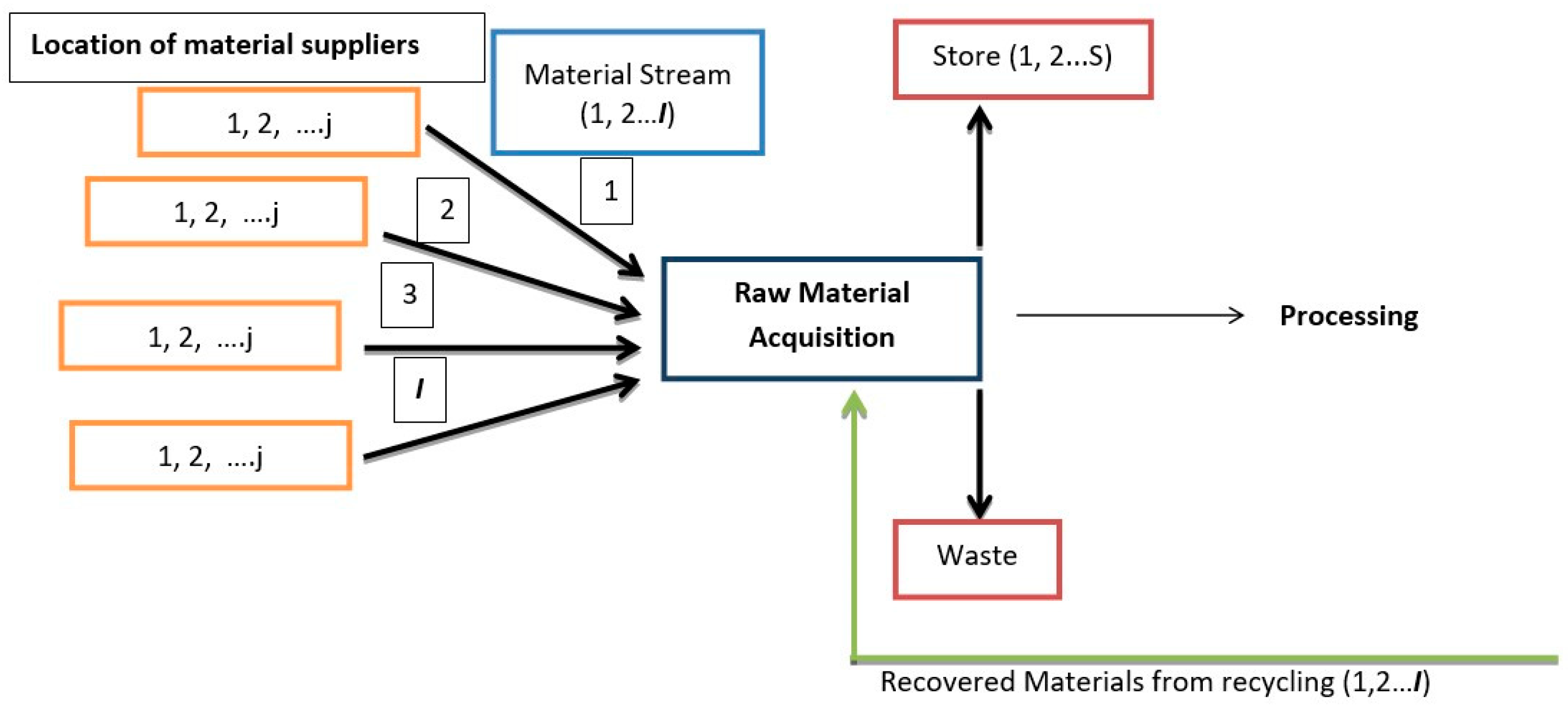
4.2.1. Environment Impact from Raw Material Acquisition (E_MA)

The following figure (Figure 5) [38] shows the flow of material needed for the NiZn battery. Here, it shows that the material $i$ can be supplied by $j$ number of suppliers from different locations.

The definition of variables used in the modeling of the environment impact function is below [58]:

1…..i…..I = Number of materials coming in.

1…..j…..J = Number of suppliers from different locations.

1…..s….S = Number of storage facilities.

ton: metric ton (tonne) = 1000 kg

E_(v,i) = Impact created by the acquisition of virgin material i (ton CO₂-e).

E_(r,i) = Impact created by the acquisition of recovered material i (ton CO₂-e).

E_(t,i) = Impact created transportation of material i (ton CO₂-e per ton of material).

E_(S,i) = Impact created storage of material i (ton CO₂-e per ton of material).

m_(i,j) = Amount (mass) of material i supplied from supplier j (ton).

d_(i,j) = Transport distance of material i supplied from supplier j by all modes of transport (km).

m_(i,s) = Amount (mass) of material i allocated to storage site s (ton).

D_(i,j) = Maximum demand of material i from supplier j (ton).

M_i = Total supply of material i (ton).

R_i = Amount (mass) of material i recovered from recycling (ton).

The environmental impact produced during material acquisition can be modeled as Equation (17).

$$E_{MA}=\sum _{i=1}^I\left[\begin{array}{c}\left({\displaystyle \sum _{j=1}^J}{m}_{i,j}\ast E_{v,i}+R_i\ast E_{r,i}\right)+\left({\displaystyle \sum _{j=1}^J}{m}_{i,j}\ast d_{i,j}\ast E_{t,i,j}\right) \\ +\left({\displaystyle \sum _{s=1}^S}{m}_{s,i}\ast E_{s,i}\right)\end{array}\right]$$

(17)

4.2.2. Environmental Impact from Manufacturing (E_m)

The environmental impact produced during manufacturing is modeled based on the EverBatt model suggested by Argonne National Laboratory [49].

The Manufacturing environmental impact model is in Equation (18),

$$E_m={\sum }_k{E}_k={\sum }_k({\sum }_i{m}_i\times E_{i,k}+{\sum }_j{Q}_j\times E_{j,k}+P_k)$$

(18)

where

$m_i$ = Mass of the material $i$ consumed in kg.

$E_k$ = Environmental Impact category $k$ [56].

$E_{i,k}$ = Environmental Impact category $k$ for 1 kg of material $i$ consumed in the process.

$Q_j$ = Quantity of Energy type $j$ consumed in MJ.

$P_k$ = GHG emission from the process.

4.2.3. Environmental Impact from Operation and Maintenance (E_O&M)

During its operational life, the battery only uses electricity to get charged; therefore, the environmental impact produced during the use phase of the battery will be easily modeled as the sum of environmental impacts due to sources of electricity generation. If there are $j$ types of energy mix used in the electric grid for supply, then environmental impact during the operation and maintenance of NiZn battery will be estimated through Equation (19).

$$E_{O\&M}=\sum _K\sum _j{Q}_j.E_{j,k}$$

(19)

where

$E_{j,k}$= Environmental Impact category $k$ for the type of energy mix $j$ in the supply to the grid.

$Q_j$= Quantity of Energy type $j$ consumed in MJ.

4.2.4. Environmental Impact of End-of-Life (E_EoL)

When batteries retire from service and are sent for dismantling at recycling facilities, it is not always possible to recover all the materials from spent batteries for reuse. Some parts of battery materials need to be disposed of through different methods like dumping them into landfills, incineration, etc. The recycling process and disposal of residuals both produce an environmental impact, and they can be modeled as Equation (20).

$$E_{EoL}=\sum _{i=1}^I{E}_{recl,i}+\sum _{i=1}^I{E}_{disp,i}$$

(20)

where $E_{recl,i}$ denotes environmental impact due to the recycling of materials $i$, and $E_{disp,i}$ denotes environmental impact due to transport and disposal of material I (see Equation (21)).

$$E_{rec,i}={(E}_{v,i}-E_{recov,i})\ast \left({\displaystyle \frac{1-{RR}_i\ast Y_i}{1-{\left({RR}_i\ast Y_i\right)}^n}}\right)+E_{recov,i}$$

(21)

where

n = number of times the recovered material can be recycled.

$E_{recov,i}$= Environmental Impact for recovering the material “$i$”.

$E\left(v, i\right)$= Impact created by the acquisition of virgin material $i$ (ton CO₂-e).

$R{R}_i$ = Recovery rate of material $i$ = ${\displaystyle \frac{amount of material recovered}{amount of material obtained}}$

$Y_i$ = Yelding rate of material $i$ = ${\displaystyle \frac{amount of material reprocessed}{amount of material recovered}}$

5. Optimizing LCCA and LCA of NiZn Batteries by MOPSO

5.1. Assumptions and Limitations

For simplicity, MOPSO was applied to phase I) “raw material acquisition” and phase IV) “end-of-life” in Figure 1 of Ref. [38]. Phase II) “Manufacturing” and Phase III) “Operation & Maintenance” are considered constant functions at the moment in the study, while costs and environmental impacts in Phase III) “Operation & Maintenance” will depend on where the user of the NiZn battery is located, and they are considered constant at the moment by the study for simplicity. As an example, Paris (France) was considered the place where NiZn batteries are manufactured, and Krefeld (Germany) was the place to recycle after EoL. The names of the materials and compositions are not disclosed in this paper due to confidentiality.

5.2. Data Related to the LCCA of NiZn Batteries

The cost data in EUR/kg of material considered for phase I) “raw material acquisition” was collected based on the top five countries around the world suppliers of these materials in the year 2021 (last information available) according to the Observatory of Economic Complexity (OEC) (https://oec.world/, accessed on 18 June 2024). According to Equation (9), this cost considers both the raw material acquisition cost (C_vi) and the transportation cost (C_{t, I, j}) of this raw material from the original country to Paris (France) as the location of the manufacturing site.

C_vi was calculated by using material supplier databases and literature. This information has been collected from Ecoinvent 3.8, Agribalyse V 1.3, Ecoinvent 3.7, and Worldsteel 2020. On the other hand, the data collected from internet sources came from Chemanalyst, WITS (World Integrated Trade Solution), and Leonland. Meanwhile, C_{t, I, j} was calculated by multiplying the distance from the original country of the raw material to the manufacturing site (Paris-France) and the “Transport unit cost“ according to

Table 1. “Transport unit cost” per each mode of transport.

	EUR/kg × km	References about the “Transport Unit Cost”
Road	0.000027	[62,63,64,65,66,67,68,69,70,71,72]
Rail	0.000036	[73,74,75,76,77]
Ship	0.0000065	[72,75,76,77,78]
Air	0.00019	[71,72,76,77,78,79,80,81]

. The multimodal journey with the lowest total cost was selected. This transportation cost was increased by 15% [57,58,59] in case the material is considered a dangerous good [59,60,61].

The costs in EUR/kg of material considered for phase iv) “end-of-life” are shown in

Table 2. Cost of “end-of-life” per material and country.

Countries	EUR/kg of Waste
USA	0.147
China	0.236
India	0.150
Brazil	0.174
Japan	0.205

. According to Equation (15), these costs are considering both the “disposal treatment fee” and the “transport costs” from the recycling site (Krefeld, Germany) to the country of disposal:

Table 2 was generated based on the top five countries around the world that are treating waste from batteries in Kg/year according to the following:

• The World Bank: data and reports on environmental and waste management.
• United Nations Environment Programme (UNEP): UNEP reports and data on global environmental issues, including waste management.
• National environmental agencies and ministries.
• Environmental organizations: Environmental Protection Agency (EPA) in the United States.

For the case of the calculation of the “disposal treatment fee” for the top five countries, the USA, China, India, Brazil and Japan, the references of [72,79,80,81,82] have been used, respectively.

The “Transport unit costs” per each mode of transport for the calculation of the “transport costs” from the recycling site (Krefeld, Germany) to the country of disposal was considered the same as for phase i) “raw material acquisition“ (Table 1); and the methodology to calculate these transportation costs was the same, in which garbage produced was considered as a dangerous good.

5.3. Data Related to the LCA of NiZn Batteries

The environmental impact data in kg CO₂-e/kg of battery mass for phase I) “raw material acquisition”, according to Equation (17), considers both the environmental impact created by the acquisition of virgin material, which was calculated by using OpenLCA (V1.11.0) in Ref. [39], and the environmental impact generated by the transport of this raw material from the original country to the manufacturing site (Paris-France), calculated from the GLEC guidelines version 3 [83] considering the multimodal journey from each original country to Paris with the lowest emission of CO₂ (

Table 3. Environmental impact of “end-of-life” per material and country [47,56].

Country	GARBAGE (kg CO2-e/kg Battery)
Brazil	0.190
China	0.287
India	0.176
Japan	0.292
United States	0.139

) [47,56]. The environmental impact created by the acquisition of virgin material is a constant in the optimization model, as it is independent of the original country, while E_m linked to transport depends on the original country.

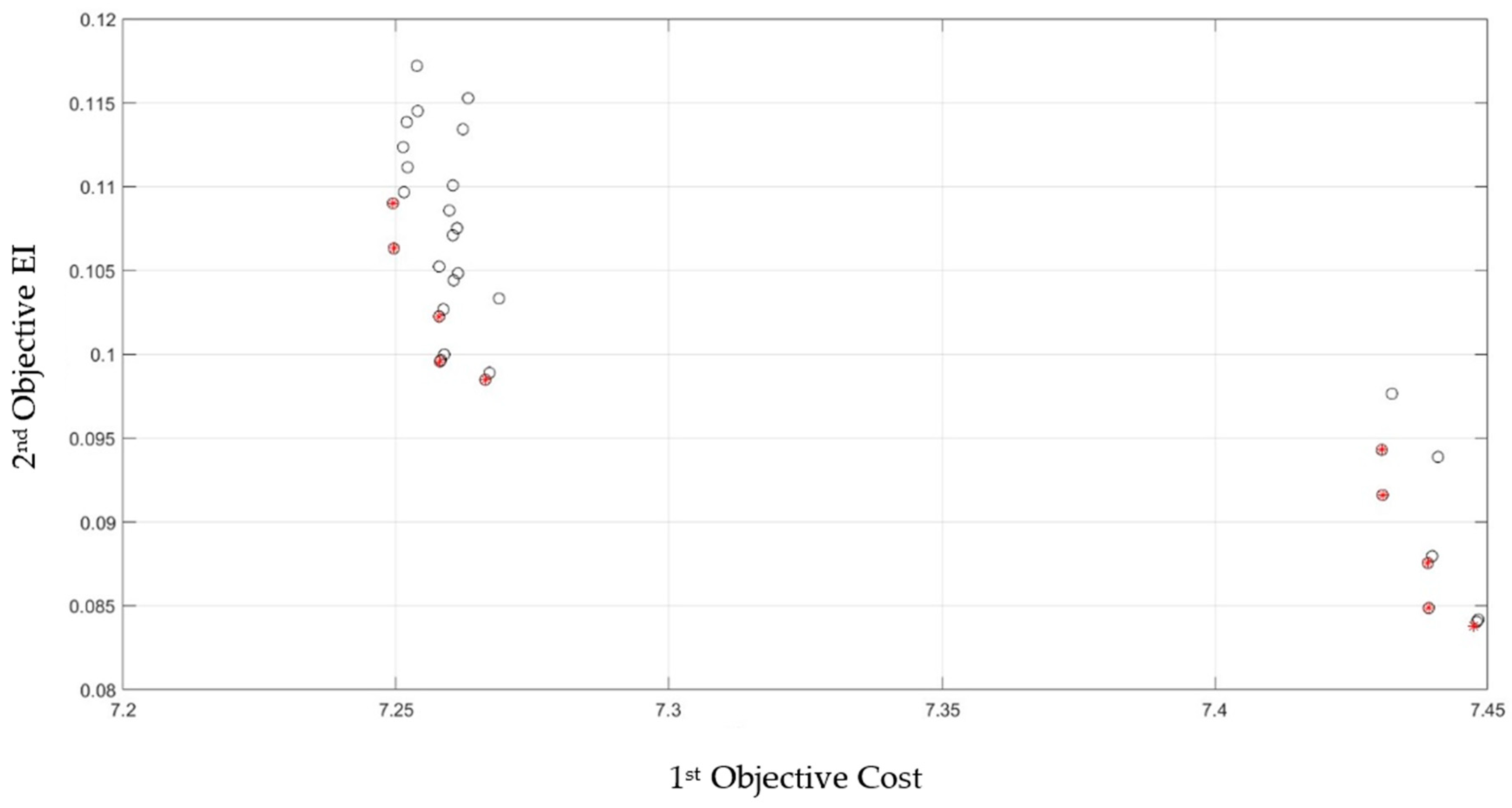
5.4. Results of Applying MOPSO to Optimize the LCA and LCCA of NiZn Batteries

An initial population of 1000 individuals, each one with a combination of two “Gens” (Material, Country), was randomly generated. Two parameters: The cost, jointly with the environmental impact, were assigned to each pair of “Gens” [47,78,79].

MOPSO algorithms were executed in MATLAB to obtain more and better individuals regarding these two parameters as defined in Equations (22) and (23).

$$Cost Individual i={\sum }_{j=1}^n\left(C_{1 j}+C_{EoL i}\right)$$

(22)

$$EI Individual \mathrm{i}={\sum }_{j=1}^n\left({E_{MA}}_j+E_{EoL i}\right)$$

(23)

where

• “$j$” is a Gen (Material, Country) belonging to the individual “$i$”, and $n$ = the total number of the gens (Material, Country) defining the individual.
• $C_{1 j}$ = Cost of raw material acquisition and transportation belonging to the couple (Material, Country) number “$j$” for the individual “$i$”
• $C_{EoL}$= Cost of final disposal of waste and transportation belonging to the couple (Garbage, Country) for the individual “$i$”.
• $E_{MA}$ = Environmental impact of the raw material acquisition and transport belonging to the couple (Material, Country) number “$j$” for the individual “$i$”
• $E_{EoL}$ = Environmental impact of final disposal of garbage and transportation belonging to the couple (Garbage, Country) for the individual “$i$”.

One thousand iterations were executed with a mutation rate = 0.5 to obtain new and better individuals “$i$” by using a screening process of keeping good individuals and removing the bad ones based on the Pareto optimal frontier by depicting all created individuals in a graph with two axes, “Cost” and “EI”, as defined in Equations (22) and (23). The values of other MOPSO parameters such as Intertia weight (w) = 1, Damping Rate (w_damp) = 0.99, Local learning Coefficient (c1) = 1, Global learning Coefficient (c2) = 1, Inflation Rate (alfa) = 0.1, Leader Selection pressure (beta) = 2 and, Deletion Selection Pressure (gamma) = 2 has been adopted as per suggestions in literature [62,63].

After these 1000 iterations,

Table 4. Combinations “Material–Country” in the Pareto optimal frontier from cradle to grave.

Solutions Serial Number	Mat. 1	Mat. 2	Mat. 3	Mat. 4	Mat. 5	Mat. 6	Mat. 7	Mat. 8	Mat. 9	Mat. 10	Mat. 11	Mat. 12	Mat. 13	Mat. 14	Landfill of Residual
1	BELGIUM’	BELGIUM’	BELGIUM’	NORWAY’	RUSSIA’	UNITED KINGDOM’	GERMANY’	SOUTH KOREA’	BELGIUM’	UNITED KINGDOM’	NETHERLANDS’	CANADA’	NETHERLANDS’	BELGIUM’	UNITED STATES’
2	BELGIUM’	BELGIUM’	MALAYSIA’	NORWAY’	RUSSIA’	UNITED KINGDOM’	GERMANY’	SOUTH KOREA’	BELGIUM’	UNITED KINGDOM’	NETHERLANDS’	CANADA’	NETHERLANDS’	BELGIUM’	UNITED STATES’
3	MALAYSIA’	BELGIUM’	BELGIUM’	NORWAY’	RUSSIA’	UNITED KINGDOM’	GERMANY’	GERMANY’	BELGIUM’	UNITED KINGDOM’	NETHERLANDS’	CANADA’	NETHERLANDS’	BELGIUM’	UNITED STATES’
4	BELGIUM’	BELGIUM’	BELGIUM’	NORWAY’	RUSSIA’	UNITED KINGDOM’	GERMANY’	SAUDI ARABIA’	BELGIUM’	UNITED KINGDOM’	NETHERLANDS’	CANADA’	NETHERLANDS’	BELGIUM’	UNITED STATES’
5	MALAYSIA’	BELGIUM’	BELGIUM’	NORWAY’	RUSSIA’	UNITED KINGDOM’	GERMANY’	SAUDI ARABIA’	BELGIUM’	UNITED KINGDOM’	NETHERLANDS’	CANADA’	NETHERLANDS’	BELGIUM’	UNITED STATES’
6	BELGIUM’	BELGIUM’	MALAYSIA’	NORWAY’	RUSSIA’	UNITED KINGDOM’	GERMANY’	SAUDI ARABIA’	BELGIUM’	UNITED KINGDOM’	NETHERLANDS’	CANADA’	NETHERLANDS’	BELGIUM’	UNITED STATES’
7	MALAYSIA’	BELGIUM’	MALAYSIA’	NORWAY’	RUSSIA’	UNITED KINGDOM’	GERMANY’	SAUDI ARABIA’	BELGIUM’	UNITED KINGDOM’	NETHERLANDS’	CANADA’	NETHERLANDS’	BELGIUM’	UNITED STATES’
8	MALAYSIA’	BELGIUM’	MALAYSIA’	NORWAY’	RUSSIA’	UNITED KINGDOM’	GERMANY’	SOUTH KOREA’	BELGIUM’	UNITED KINGDOM’	NETHERLANDS’	CANADA’	NETHERLANDS’	BELGIUM’	UNITED STATES’
9	BELGIUM’	BELGIUM’	BELGIUM’	NORWAY’	RUSSIA’	UNITED KINGDOM’	GERMANY’	GERMANY’	BELGIUM’	UNITED KINGDOM’	NETHERLANDS’	CANADA’	NETHERLANDS’	BELGIUM’	UNITED STATES’
10	MALAYSIA’	BELGIUM’	BELGIUM’	NORWAY’	RUSSIA’	UNITED KINGDOM’	GERMANY’	SOUTH KOREA’	BELGIUM’	UNITED KINGDOM’	NETHERLANDS’	CANADA’	NETHERLANDS’	BELGIUM’	UNITED STATES’

shows the optimized combination of raw material suppliers and waste residual disposal location for NiZn batteries, and their corresponding values are presented in

Table 5. Ten optimal Cost and EI values of NiZn F2 obtained and presented in Pareto front.

Serial Number of Individual	Production and Waste Disposal COST (EUR/kg of Battery Mass)	Production and Waste Disposal EI (kg CO2-e/kg of Battery Mass)
1	7.439	0.088
2	7.431	0.094
3	7.266	0.098
4	7.439	0.085
5	7.258	0.100
6	7.431	0.092
7	7.250	0.106
8	7.249	0.109
9	7.447	0.084
10	7.258	0.102

. Taking into account MOPSO parameters, we can receive up to 10 optimal solutions. Table 4 and Table 5 show 10 optimal solutions obtained from MOPSO, which are numbered 1 to 10 for combined understanding.

Figure 6 depicts the actual Pareto fronts obtained. In each iteration, from the initial population of 1000 individuals, non-dominated solutions were saved in the repository, and with mutation, new and better populations were generated. In further iterations, among the mutated population generated in the immediate last iteration, if there are better non-dominated individuals were found, the already existing non-dominated individual stored in the repository had been replaced; otherwise, the individual in the repository remains the same. This search operation stops at the 1000th iteration. The black circles in the Pareto front shown in Figure 6 are those individuals who have survived after 1000 mutations, and the red stars are those non-dominated solutions saved in the repository during the process of 1000 mutations.

6. Validation of the Model

6.1. Sensitivity Analysis

In the following table (

Table 6. Results of sensitivity analysis.

Material	Original Results	Results after 5% Increase	Results after a 5% Decrease	Percentage of Matching Results
Material 1	Belgium	Belgium	Malaysia	50%
	Malaysia	Malaysia	Netherlands
Material 2	Belgium	Belgium	Belgium	100%
Material 3	Belgium	Belgium	Belgium	100%
	Malaysia	Malaysia	Malaysia
Material 4	Norway	Norway	Norway	100%
Material 5	Russia	Russia	Russia	100%
Material 6	United Kingdom	United Kingdom	United Kingdom	100%
Material 7	Germany	Germany	Germany	100%
Material 8	South Korea	Saudi Arabia	Saudi Arabia	70%
	Germany	South Korea	South Korea
	Saudi Arabia
Material 9	Belgium	Belgium	Belgium	100%
Material 10	United Kingdom	United Kingdom	Italy	0
Material 11	Netherlands	Netherlands	Netherlands	100%
Material 12	Canada	Canada	Canada	100%
Material 13	Netherlands	Netherlands	Netherlands	100%
Material 14	Belgium	Belgium	Netherlands	0
			The overall percentage of matching results:	80%

), the results of the sensitivity analysis are presented. This table describes an analysis according to the original results derived from AI (MOPSO), a 5% increase and decrease in cost and environmental impact, and finally, the percentage of matching results. As a result, the average value for sensitivity analysis in this study is equal to 80%. This sensitivity analysis shows the robustness of the AI model developed in this study.

6.2. Robustness Regarding the Mathematical Parameters

In the sensitivity analysis, five tests were performed with 1000 iterations and 100 initial populations and five tests with the same parameters and the number of iterations as before, but this time with 1000 initial populations and one test with the same parameters and number of iterations but 10,000 initial populations. The idea behind several tests with an increased initial population was to realize the accuracy of results while repeating the tests. We compared the results obtained from these tests with the final result (Table 4) mentioned per each material and supplier country. By performing these repeated tests, we have realized that although small variations in the MOPSO parameters are not affecting the final results in our case, increasing the numbers of initial populations increases the accuracy of results on the cost of increased runtime of the MATLAB algorithm.

The MATLAB algorithm runtime was 3–4 min per test when the initial number of populations was 100 individuals. The five results obtained on this set of parameters are compared and concluded that for Mat. 1, Table 4 suggested the most economical and environmentally friendly suppliers are Malaysia and the Netherlands 5 times each in 10 optimum solutions. The sensitivity analysis, Tests 1, 4, and 5 suggested Malaysia and the Netherlands each 50–50% times, whereas Tests 2 and 3 suggested Malaysia and Belgium each an equal number of times (50–50%). Therefore, considering the results from all 5 tests, we obtained a total of 48 optimum solutions, of which (For Mat. 1) 50% were Malaysia, 31.25% were the Netherlands, and 18.75% of the results suggested Belgium. For Mat. 2, all the optimum solutions from Tests 1 to 4 have suggested Belgium, and all the optimum solutions from Test 5 have suggested the United States. In total, 38 out of 48 (79.16%) optimal solutions suggested Belgium, which is also suggested in Table 4. Therefore, we can conclude that the accuracy of results is around 80% when tests are repeated after taking the initial populations of 100 individuals.

The other set of five tests with an initial population of 1000 individuals takes 15–17 min runtime per test, but the accuracy of results improved significantly. A total of 49 optimal solutions were obtained by these five results and presented in Table 4. For material Mat. 1, considering all five results, 25 optimal solutions have suggested Belgium, and the other 24 have suggested Malaysia (51–49%), which is very similar to the final result in Table 4, which suggested Belgium–Malaysia 5–5 time each in those 10 optimal solutions. Comparing the optimal locations for Mat. 3, the Belgium–Malaysia pair has been suggested 22 times each in all 49 optimal solutions from five tests, which is 45%, and the other five solutions have suggested the United Kingdom, whereas Table 4 suggested 60% Belgium and 40% Malaysia. Comparing the results from Table 4 with the Test 1 results of sensitivity analysis, we observed more than 95% similarities in the results. The last test with 10,000 initial populations took a huge 3 h and 22 min runtime and had around similarity in the optimal solutions obtained in Table 4 and Test 1 results of sensitivity analysis.

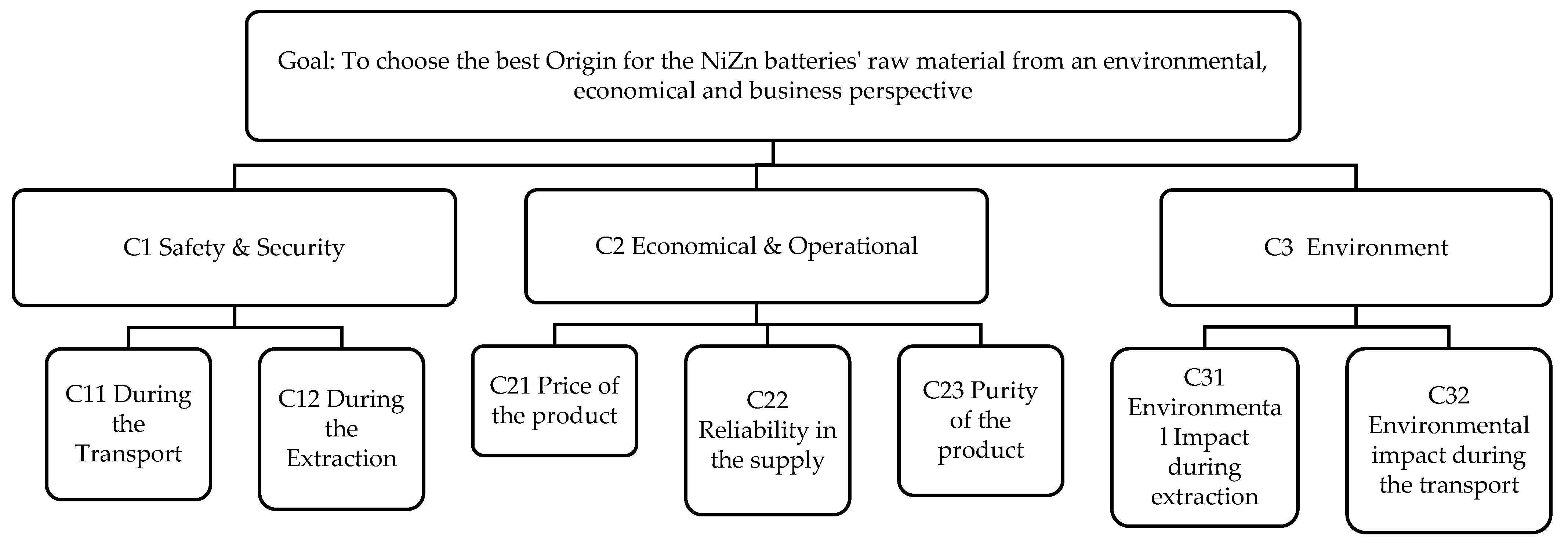
6.3. Validation through the AHP

The qualitative validation of MOPSO results has been performed by applying the AHP (Analytic Hierarchy Process) and through an expert panel as per the suggested methodology in the literature [84,85,86]. The AHP is applied to obtain a weighted hierarchy of factors with an influence on the goal [87,88,89] “Choosing the best Origin for the NiZn batteries’ raw material from an environmental, economic, and business perspective”.

To optimize the effort from the expert panel by filling multiple pairwise comparison matrixes, the AHP analysis is focused on the three raw materials that represent more than 50% of the weights of batteries (Material 6, 13, and 5) and three materials according to the optimization of cost and environmental impacts through the AI model (Material 1, 3, and 8) in ten solutions. This analysis is performed to determine which countries are the most appropriate according to the global weights to establish the most efficient supply chain for battery materials (see

Table 7. List of raw materials of NiZn batteries and their associated countries.

NiZn Raw Materials	List of Countries
Material 6	A1-Canada, A2-China, A3-Japan, A4-United Kingdom, A5-Australia
Material 13	A1-Australia, A2-Canada, A3-Netherlands, A4-South Korea, A5-Spain
Material 5	A1-Chile, A2-Japan, A3-Kazakhstan, A4-Congo, A5-Russia
Material 1	A1-Belgium, A2-Chinese Taipei, A3-Malaysia, A4-Netherlands, A5-South Korea
Material 3	A1-Belgium, A2-China, A3-Germany, A4-Malaysia, A5-United Kingdom
Material 8	A1-Germany, A2-Saudi Arabia, A3-South Korea, A4-United Arab Emirates, A5-USA

).

A hierarchical model in two levels was prepared (see Figure 7) with factors generated and validated by a multidisciplinary panel shaped by the following:

• Entity: Orange, Country: France, Position of the member: Engineer in charge of energy storage studies
• Entity: Chaowei Power Co. LTD, Country: China, Position of the member: Vice President‘s Assistant
• Entity: Naval Group, Country: France, Position of the member: Research and Innovation Manager
• Entity: EDP LABELEC, Country: Portugal, Position of the member: R&D Engineer and Project Manager
• Entity: ZSW, Country: Germany, Position of the member: Scientist and team leader
• Entity: SUNERGY, Country: France, Position of the member: R&D Deputy Manager
• Entity: SUPERGRID, Country: France, Position of the member: Research and development engineer
• Entity: UNIGE, Country: Italy, Position of the member: Researcher and Assistant Professor

This hierarchical model is applied to all six materials presented in Table 7 individually.

After the expert panel validated the hierarchical models, pairwise comparison matrices were introduced. The aim of preparing this matrix is to compare the importance between criteria levels 1 and 2. This matrix aims to assess the expert panel‘s technical opinion to determine which criteria are more important in achieving the main goal and how much this ratio is according to the scale of Saaty [90,91]. The AHP analysis is focused on the three raw materials that represent more than 50% of the weights of batteries and another three materials according to the optimization of cost and environmental impacts through the AI model in ten solutions. This analysis is performed to evaluate which countries are the most appropriate according to the global weights to establish the most efficient supply chain for battery materials. The criteria, which are presented in Figure 7, were determined by microscopic analysis of technical and business risks affecting the security of the supply of NiZn battery raw materials.

Taking into account the results derived from MOPSO output for six raw materials of Materials 6, 13, 5, 1, 3, and 8 and combinations “Material–Country” in the Pareto optimal frontier from cradle to grave (Table 4) and consequently comparing this result with the result of AHP analysis, the following findings have been achieved. As per

Table 8. Deviation between AI outputs and AHP analysis.

Materials	Countries Chosen by AI (MOPSO)	Countries Chosen by AHP (Human Factor)
		Country	Weight	Rank
Material 6	United Kingdom	Canada	0.225	1
		United Kingdom	0.222	2
		Japan	0.196	3
		China	0.191	4
		Australia	0.167	5
Material 13	Netherlands	Netherlands	0.245	1
		Spain	0.231	2
		Australia	0.191	3
		Canada	0.185	4
		South Korea	0.147	5
Material 5	Russia	Japan	0.260	1
		Chile	0.254	2
		Kazakhstan	0.175	3
		Congo	0.169	4
		Russia	0.142	5
Material 1	Belgium	Belgium	0.306	1
		Netherlands	0.263	2
		South Korea	0.158	3
	Malaysia	Malaysia	0.149	4
		Chinese Taipei	0.125	5
Material 3	Belgium	Belgium	0.266	1
		Germany	0.226	2
		China	0.190	3
	Malaysia	United Kingdom	0.183	4
		Malaysia	0.134	5
Material 8	South Korea	Germany	0.393	1
		South Korea	0.180	2
	Germany	USA	0.173	3
		Saudi Arabia	0.128	4
	Saudi Arabia	United Arab Emirates	0.126	5

, the list of countries chosen by AI and AHP has similarities. However, for the case of the data collected for Material 5, the AI chose Russia. The main reason for this selection was that the data used and applied in AI (MOPSO) were collected before the invasion of Ukraine by Russia. On the other hand, as it is presented by the results of AHP, for Material 5, Russia is placed in the fifth rank. This is due to the fact that the results of pairwise comparison matrices were collected after the invasion, and the expert panel preferred to give low scores to Russia. In this case, instead of Russia, Japan, which is placed in the first rank, can be chosen as an appropriate alternative [92]. It is important to note that the AHP is primarily focused on validating the results obtained from AI algorithms rather than on proving or gaining new insights from data or analyzing the data.

7. Improvement of Some Sustainability KPIs

The sustainability KPIs selected in this study to assess the impact of the optimization model were the following: “capital cost (EUR/kWh)”, “storage cost (EUR/kWh)”, “end-of-life cost (EUR/kWh)”, and “global warming potential (GWP)” (kg-CO₂-e/MWh) [93]. The evolution of these sustainability KPIs before and after the optimization model is presented in

Table 9. Evolution of relevant sustainability KPIs during the Lolabat project included in the optimization model [38,39].

KPIs	Before Applying the Optimization Model	After Applying the Optimization Model	Achieved Results	Target
Capital cost (EUR/kWh)	0.0511 EUR/kWh	0.0450 EUR/kWh	11.96%	20–30% decrease
Storage cost (EUR/kWh)	0.000638 (EUR/kWh)	0.000562 (EUR/kWh)	11.96%	20–35% decrease
End-of-life cost (EUR/kWh)	0.00549 (EUR/kWh)	0.00529 (EUR/kWh)	3.65%	10% decrease
Global Warming Potential (kg-CO2-e/MWh)	7.168 kg-CO2-e/MWh	5.241 kg-CO2-e/MWh	26.88%	15% decrease

. Results showed an 11.96% reduction in capital cost and storage cost and a 26.8% decrease in GWP. With the application of MOPSO, the optimized waste disposal cost decreased by 37.75%. Since the contribution of waste disposal cost to the total amount of EoL cost is 10.6%, a 3.65% decrease in the net EoL cost KPI has therefore been achieved.

8. Limitations and Assumptions

Finally, before concluding our study, it is worth mentioning that certain limitations and assumptions have been made to simplify the modeling process. These limitations emerge from the fact that the NiZn battery is still in the research and development stage and that there are only laboratory-scale observations available. The primary life cycle inventory (LCI) data for cradle-to-gate production was gathered from a pilot-scale production that solely used electricity. As a result, the energy demand was significantly higher than that of a regulated and mature production, which was used as a comparative basis for this study. And this is the reason, as mentioned in Section 5, that we consider the manufacturing and operational phase of the battery as constant in the optimization algorithm. However, the programming of these phases has been made dynamic so that in the future, we will have enough data to consider it. Due to the confidentiality of the patent [94], we reframed to disclose the name of materials and their composition in nickel-zinc batteries in Table 4 of this paper.

9. Conclusions

This study has attempted to optimize the life cycle, environmental impact, and cost of NiZn battery, taking into account the latest data available. Environmental impact and cost data used in this study have been adopted from the development according to Refs. [38,39]. Initially, the genetic algorithm (GA) was proposed for optimization, but it was found to be slow with many variables. After comparing available algorithms, the study concluded that MOPSO is more suitable for multi-objective optimization than GA.

This study uses constant battery parameters like material composition, energy density, and cycle life while adopting the latest data from NiZn batteries. The environmental impact (Global Warming Potential) and cost of raw materials from the top five producers and waste treatment locations are considered variables. Manufacturing is set in Paris, France, and recycling in Krefeld, Germany, as constraints. The analysis includes 14 material streams and one waste disposal line from 36 different global locations, each with varying costs and environmental impacts.

The MOPSO results identify optimal supplier locations for raw materials with minimal cost and environmental impact, as well as optimal waste disposal locations for non-recyclable materials. Among the ten optimal solutions, a single solution is recommended for 11 out of 14 materials, as well as for waste disposal and treatment locations.

Based on all ten optimal solutions and given that NiZn’s production location is in Paris, it can be concluded that Belgium would be the best supplier for Mat. 2, Mat. 9, and Mat. 14. The United Kingdom is the preferred supplier of Mat. 6 and Mat. 10, whereas the Netherlands must be preferred for Mat. 13 and Mat. 11. For Mat. 5, Mat. 4, Mat. 7, and Mat. 12, Russia, Norway, Germany, and Canada are the preferred suppliers, respectively. Residual wastes obtained from spent batteries can be best treated in the United States. The Netherlands and Malaysia are two optimal suppliers for Mat. 1, whereas Belgium and Malaysia would be better suppliers for Mat. 3. Three options were considered optimal for the supply of Mat. 8; they are Germany, Saudi Arabia, and South Korea. The algorithm developed in this study can be used for further formulations of NiZn batteries to obtain optimum cost and environmental impact by just providing the battery parameters.

A comparison between the countries that were chosen by AI (MOPSO) and the countries that were chosen in AHP analysis by an expert panel survey has been performed in this study, and it has been found that there is a significant similarity in the results of the countries chosen by both methods. The AI model in this study demonstrates robustness through coherence with AHP analysis and resilience to market fluctuations in the sensitivity analysis. Post-optimization, significant reductions in NiZn‘s global warming potential validate the AI model‘s effectiveness.

The manufacturing, operation, and maintenance aspects of the NiZn battery life cycle are currently treated as constant in AI algorithms. As further developments are made to optimize the life cycle environmental impacts and costs of NiZn batteries, it is important to include these aspects in the programming modules as dynamic for estimating sustainability Key Performance Indicators (KPIs) and for the AHP validations, similar to how it has been done for raw material acquisition and waste disposal phases.

References

1. Filimonau, V. Life cycle assessment. In The Routledge Handbook of Tourism and Sustainability; Routledge: Abingdon, UK, 2015; Volume 45, pp. 209–220. [Google Scholar]
2. SETAC. Guidelines for Life-Cycle Impact Assessment: Code of Practice; Society of Environmental Toxicology and Chemistry: Washington, DC, USA, 1993; Volume 1, p. 73. Available online: https://www.setac.org/resource/guidelines-lca-code-practice-1993.html (accessed on 18 June 2024).
3. Fava, J.; Consoli, F.; Denison, R.; Dickson, K.; Mohin, T.; Vigon, B. A Conceptual Framework for Life-Cycle Impact Assessment; Society of Environmental Toxicology and Chemistry: Washington, DC, USA, 1993; pp. 1–160. [Google Scholar]
4. Guinée, J.B.; Heijungs, R.; Huppes, G.; Zamagni, A.; Masoni, P.; Buonamici, R.; Ekvall, T.; Rydberg, T. Life Cycle Assessment: Past, Present, and Future. Environ. Sci. Technol. 2011, 45, 90–96. [Google Scholar] [CrossRef]
5. ISO 14040; Environmental Assessment—Life Cycle Assessment—Principles and Framework. Internation Standard Organisation: Geneva, Switzerland, 2009; Volume 1997, pp. 1–20.
6. Azapagic, A.; Clift, R. The application of life cycle assessment to process optimisation. Comput. Chem. Eng. 1999, 23, 1509–1526. [Google Scholar] [CrossRef]
7. Cerda-Flores, S.C.; Rojas-Punzo, A.A.; Nápoles-Rivera, F. Applications of Multi-Objective Optimization to Industrial Processes: A Literature Review. Processes 2022, 10, 133. [Google Scholar] [CrossRef]
8. Deng, C.; Li, Z.; Shao, X.; Zhang, C. Integration and optimization of LCA and LCC to eco-balance for mechanical product design. In Proceedings of the World Congress on Intelligent Control and Automation (WCICA), Chongqing, China, 25–27 June 2008; IEEE: New York, NY, USA; pp. 1085–1090. [Google Scholar] [CrossRef]
9. Yu, B.; Gu, X.; Ni, F.; Guo, R. Multi-objective optimization for asphalt pavement maintenance plans at project level: Integrating performance, cost and environment. Transp. Res. Part D Transp. Environ. 2015, 41, 64–74. [Google Scholar] [CrossRef]
10. Brunet, R.; Cortés, D.; Guillén-Gosálbez, G.; Jiménez, L.; Boer, D. Minimization of the LCA impact of thermodynamic cycles using a combined simulation-optimization approach. Appl. Therm. Eng. 2012, 48, 367–377. [Google Scholar] [CrossRef]
11. Pieragostini, C.; Mussati, M.C.; Aguirre, P. On process optimization considering LCA methodology. J. Environ. Manag. 2012, 96, 43–54. [Google Scholar] [CrossRef]
12. Yu, B.; Lu, Q.; Xu, J. An improved pavement maintenance optimization methodology: Integrating LCA and LCCA. Transp. Res. Part A Policy Pr. 2013, 55, 1–11. [Google Scholar] [CrossRef]
13. Ribau, J.P.; Silva, C.M.; Sousa, J.M. Efficiency, cost and life cycle CO2 optimization of fuel cell hybrid and plug-in hybrid urban buses. Appl. Energy 2014, 129, 320–335. [Google Scholar] [CrossRef]
14. Movahed, Z.P.; Kabiri, M.; Ranjbar, S.; Joda, F. Multi-objective optimization of life cycle assessment of integrated waste management based on genetic algorithms: A case study of Tehran. J. Clean. Prod. 2020, 247, 119153. [Google Scholar] [CrossRef]
15. Wang, Q.; Liu, W.; Yuan, X.; Tang, H.; Tang, Y.; Wang, M.; Zuo, J.; Song, Z.; Sun, J. Environmental impact analysis and process optimization of batteries based on life cycle assessment. J. Clean. Prod. 2018, 174, 1262–1273. Available online: https://www.sciencedirect.com/science/article/pii/S0959652617327178 (accessed on 18 June 2024). [CrossRef]
16. Elzein, H.; Dandres, T.; Levasseur, A.; Samson, R. How can an optimized life cycle assessment method help evaluate the use phase of energy storage systems? J. Clean. Prod. 2019, 209, 1624–1636. Available online: https://www.sciencedirect.com/science/article/pii/S0959652618334796 (accessed on 18 June 2024). [CrossRef]
17. Rossi, F.; Heleno, M.; Basosi, R.; Sinicropi, A. Environmental and economic optima of solar home systems design: A combined LCA and LCC approach. Sci. Total. Environ. 2020, 744, 140569. [Google Scholar] [CrossRef] [PubMed]
18. Rossi, F.; Tosti, L.; Basosi, R.; Cusenza, M.A.; Parisi, M.L.; Sinicropi, A. Environmental optimization model for the European batteries industry based on prospective life cycle assessment and material flow analysis. Renew. Sustain. Energy Rev. 2023, 183, 113485. Available online: https://www.sciencedirect.com/science/article/pii/S1364032123003428 (accessed on 18 June 2024). [CrossRef]
19. Fahimi, A.; Solorio, H.; Nekouei, R.K.; Vahidi, E. Analyzing the environmental impact of recovering critical materials from spent lithium-ion batteries through statistical optimization. J. Power Sources 2023, 580, 233425. [Google Scholar] [CrossRef]
20. ICRON. Optimization vs. Heuristics: Which is the Right Approach for Your Business? Available online: https://www.icrontech.com/resources/blogs/optimization-vs-heuristics-which-is-the-right-approach-for-your-business (accessed on 13 May 2024).
21. Heuristic (Computer Science). Available online: https://en.wikipedia.org/wiki/Heuristic_(computer_science) (accessed on 13 May 2024).
22. Huang, M.; Dong, Q.; Ni, F.; Wang, L. LCA and LCCA based multi-objective optimization of pavement maintenance. J. Clean. Prod. 2021, 283, 124583. [Google Scholar] [CrossRef]
23. Lones, M.A. Metaheuristics in nature-inspired algorithms. In Proceedings of the GECCO 2014—Companion Publication of the 2014 Genetic and Evolutionary Computation Conference, Vancouver, BC, Canada, 12–16 July 2014; ACM Press: New York, NY, USA, 2014; pp. 1419–1422. [Google Scholar] [CrossRef]
24. Reeves, C.; Rowe, J.E. GENETIC ALGORITHMS Part A: Background. In Genetic Algorithms: Principles and Perspectives; Springer: Berlin/Heidelberg, Germany, 2013; p. 28. [Google Scholar]
25. Available online: https://www.scribd.com/document/373798705/Goldberg-Genetic-Algorithms-in-Search-pdf (accessed on 18 June 2024).
26. Coello, C.A.C.; Toscano-Pulido, G.T.; Lechuga, M.S. Handling Multiple Objectives with Particle Swarm Optimization. IEEE Trans. Evol. Comput. 2004, 8, 256–279. [Google Scholar] [CrossRef]
27. Schaffer, J. Multiple Objective Optimization with Vector Evaluated Genetic Algorithms. In Proceedings of the First International Conference on Genetic Algortihms; Grefensette, G.J.E., Lawrence Erlbraum, J.J., Eds.; Routledge: London, UK, 1985; pp. 93–100. [Google Scholar]
28. Rosenberg, R. Simulation of genetic populations with biochemical properties. Math. Biosci. 1970, 8, 1–37. [Google Scholar] [CrossRef]
29. Antoniucci, G.A.; Bentley, P.J. Analysis of the Distribution of Pareto Optimal Solutions on various Multi-Objective Evolutionary Algorithms. Bachelor’s Thesis, Universitat Politècnica de Cataluny, Barcelona, Spain, 2016; pp. 1–99. [Google Scholar]
30. Zitzler, E.; Thiele, L. Multiobjective Evolutionary Algorithms: A Comparative Case Study and the Strength Pareto Approach. IEEE Trans. Evol. Comput. 1999, 3, 257–271. [Google Scholar] [CrossRef]
31. Wolpert, D.H.; Macready, W.G. No free lunch theorems for optimization. IEEE Trans. Evol. Comput. 1997, 1, 67–82. [Google Scholar] [CrossRef]
32. James, K.; Russell, E. Particle Swarm Optimization; Academic Press Professional (APP): Cambridge, MA, USA, 1996; pp. 1942–1948. [Google Scholar]
33. Heris, M.K. Mostapha Kalami Heris, Mostapha Kalami Heris, Multi-Objective PSO in MATLAB. Yarpiz. 2015. Available online: https://yarpiz.com/59/ypea121-mopso (accessed on 18 June 2024).
34. Aivaliotis-Apostolopoulos, P.; Loukidis, D. Swarming genetic algorithm: A nested fully coupled hybrid of genetic algorithm and particle swarm optimization. PLoS ONE 2022, 17, e0275094. [Google Scholar] [CrossRef]
35. Papazoglou, G.; Biskas, P. Review and Comparison of Genetic Algorithm and Particle Swarm Optimization in the Optimal Power Flow Problem. Energies 2023, 16, 1152. [Google Scholar] [CrossRef]
36. Yang, Y.; Liao, Q.; Wang, J.; Wang, Y. Application of multi-objective particle swarm optimization based on short-term memory and K-means clustering in multi-modal multi-objective optimization. Eng. Appl. Artif. Intell. 2022, 112, 104866. [Google Scholar] [CrossRef]
37. Knowles, J.D.; Corne, D.W. Approximating the nondominated front using the Pareto Archived Evolution Strategy. Evol. Comput. 2000, 8, 149–172. [Google Scholar] [CrossRef]
38. Malviya, A.K.; Malekzadeh, M.Z.; Santarremigia, F.E.; Molero, G.D.; Villalba-Sanchis, I.; Yepes, V. A Formulation Model for Computations to Estimate the Lifecycle Cost of NiZn Batteries. Sustainability 2024, 16, 1965. [Google Scholar] [CrossRef]
39. Malviya, A.K.; Malekzadeh, M.Z.; Li, J.; Li, B.; Santarremigia, F.E.; Molero, G.D.; Sanchis, I.V.; Yepes, V. A Formulation Model to Compute the Life Cycle Environmental Impact of NiZn Batteries from Cradle to Grave. Energies 2024, 17, 2751. [Google Scholar] [CrossRef]
40. IEC 60300-3-3-2017; Gestión de la Confiabilidad Parte 3-3: Guía de Aplicación Cálculo del Coste del Ciclo de Vida. European Committee for Electrotechnical Standardization: Brussels, Belgium, 2017.
41. ISO 14044; Environmental Management-Life Cycle Assessment-Requirements and Guidelines Management Environnemental-Analyse du Cycle de Vie-Exigences et Lignes Directrices. The International Organization for Standardization: Geneva, Switzerland, 2006; Volume 2006, p. 7. Available online: https://www.saiglobal.com/PDFTemp/Previews/OSH/iso/updates2006/wk26/ISO_14044-2006.PDF (accessed on 18 June 2024).
42. Nagapurkar, P.; Smith, J.D. Techno-economic optimization and environmental Life Cycle Assessment (LCA) of microgrids located in the US using genetic algorithm. Energy Convers. Manag. 2018, 181, 272–291. [Google Scholar] [CrossRef]
43. Battke, B.; Schmidt, T.S.; Grosspietsch, D.; Hoffmann, V.H. A review and probabilistic model of lifecycle costs of stationary batteries in multiple applications. Renew. Sustain. Energy Rev. 2013, 25, 240–250. [Google Scholar] [CrossRef]
44. Larsson, P.; Borjesson, P. Cost Models for Battery Energy Storage Systems; kTH Industrial Engineering and Management: Stockholm, Sweden, 2018; p. 31. Available online: http://www.diva-portal.org/smash/record.jsf?pid=diva2%3A1294152&dswid=2991 (accessed on 18 June 2024).
45. Mehdijev, S. Dimensioning and Life Cycle Costing of Battery Storage System in Residential Housing—A Case Study of Local System Operator Concept. 2017. Available online: https://www.diva-portal.org/smash/get/diva2:1130036/FULLTEXT01.pdf (accessed on 18 June 2024).
46. Schmidt, O.; Melchior, S.; Hawkes, A.; Staffell, I. Projecting the Future Levelized Cost of Electricity Storage Technologies. Joule 2019, 3, 81–100. [Google Scholar] [CrossRef]
47. Poonpun, P.; Jewell, W.T. Analysis of the cost per kilowatt hour to store electricity. IEEE Trans. Energy Convers. 2008, 23, 529–534. [Google Scholar] [CrossRef]
48. Mongird, K.; Viswanathan, V.; Balducci, P.; Alam, J.; Fotedar, V.; Koritarov, V.; Hadjerioua, B. An Evaluation of Energy Storage Cost and Performance Characteristics. Energies 2020, 13, 3307. [Google Scholar] [CrossRef]
49. Peters, M.S.; Timmerhaus, K.D. Plant Design and Economics for Chemical Engineers, 4th ed.; McGraw-Hill: New York, NY, USA, 1991; Volume 11. [Google Scholar]
50. AITEC. LOLABAT Project, Deliverable D 5.3. Report on Life Cycle Analysis (LCA) of NiZn Battery; AITEC: Valencia, Spain, 2023. [Google Scholar]
51. Rahman, M.; Oni, A.O.; Gemechu, E.; Kumar, A. The development of techno-economic models for the assessment of utility-scale electro-chemical battery storage systems. Appl. Energy 2021, 283, 116343. [Google Scholar] [CrossRef]
52. Schoenung, S.M.; Hassenzahl, W. Long vs. Short-Term Energy Storage: Sensitivity Analysis A Study for the DOE Energy Storage Systems Program. Analysis 2007, 42. Available online: https://www.researchgate.net/publication/268441140_Long-vs_Short-Term_Energy_Storage_Technologies_Analysis_A_Life-Cycle_Cost_Study_A_Study_for_the_DOE_Energy_Storage_Systems_Program (accessed on 18 June 2024).
53. Marchi, B.; Pasetti, M.; Zanoni, S. Life Cycle Cost Analysis for BESS Optimal Sizing. Energy Procedia 2017, 113, 127–134. [Google Scholar] [CrossRef]
54. McCarthy, L.; Delbosc, A.; Currie, G.; Molloy, A. Factors influencing travel mode choice among families with young children (aged 0–4): A review of the literature. Transp. Rev. 2017, 37, 767–781. [Google Scholar] [CrossRef]
55. Lima, M.C.C.; Pontes, L.P.; Vasconcelos, A.S.M.; de Araujo Silva Junior, W.; Wu, K. Economic Aspects for Recycling of Used Lithium-Ion Batteries from Electric Vehicles. Energies 2022, 15, 2203. [Google Scholar] [CrossRef]
56. Goedkoop, M.; Heijungs, R.; Huijbregts, M.; De Schryver, A.; Struijs, J.; Van Zelm, R. ReCiPe 2008. Potentials 2009, First edition, pp. 1–44. Available online: https://www.researchgate.net/publication/230770853_Recipe_2008 (accessed on 18 June 2024).
57. Alfaro-Algaba, M.; Ramirez, F.J. Techno-economic and environmental disassembly planning of lithium-ion electric vehicle battery packs for remanufacturing. Resour. Conserv. Recycl. 2020, 154, 104461. [Google Scholar] [CrossRef]
58. Mathur, N.; Sutherland, J.W.; Singh, S. A study on end of life photovoltaics as a model for developing industrial synergistic networks. J. Remanufacturing 2022, 12, 281–301. [Google Scholar] [CrossRef]
59. Dangerous Goods Shipping: Types & Best Ways to Ship [2022 Guide]. Available online: https://www.container-xchange.com/blog/dangerous-goods-shipping/ (accessed on 30 April 2024).
60. Transport of Dangerous Goods—WorkSafe ACT. Available online: https://www.worksafe.act.gov.au/health-and-safety-portal/safety-topics/dangerous-goods-and-hazardous-substances/transport-of-dangerous-goods (accessed on 30 April 2024).
61. Shipping Dangerous Goods: Rules for Different Types of Transport—GOV.UK. Available online: https://www.gov.uk/shipping-dangerous-goods/rules-for-different-types-of-transport (accessed on 30 April 2024).
62. Road Transport Price Index March 2024—Transport Exchange Group. Available online: https://transportexchangegroup.com/road-transport-price-index/ (accessed on 30 April 2024).
63. Upply. Q2-2022-Ti-Upply-IRU-The-European-Road-Freight-Rate-Benchmark; Upply: Levallois-Perret, France, 2022. [Google Scholar]
64. ITF. Key Transport Statistics 2023 (2022 Data). Available online: https://www.itf-oecd.org/key-transport-statistics-2023-2022-data (accessed on 30 April 2024).
65. International Trade in Goods by Mode of Transport—Statistics Explained. Available online: https://ec.europa.eu/eurostat/statistics-explained/index.php?title=International_trade_in_goods_by_mode_of_transport (accessed on 30 April 2024).
66. Transport—Our World in Data. Available online: https://ourworldindata.org/transport (accessed on 30 April 2024).
67. Brown, J.; Englert, D.; Hoffmann, J. International Transport Costs: Why and How to Measure Them? 2021. Available online: https://blogs.worldbank.org/en/transport/international-transport-costs-why-and-how-measure-them (accessed on 18 June 2024).
68. Priyanka Babu. What Is Transportation Cost and How to Calculate It? 2023. Available online: https://blog.tatanexarc.com/logistics/what-is-transportation-cost/ (accessed on 18 June 2024).
69. Plane, P. What Factors Drive Transport and Logistics Costs in Africa? J. Afr. Econ. 2021, 30, 370–388. [Google Scholar] [CrossRef]
70. Suarez, J.P.; Lagonera, M.J.; Ueno, R.; Sinarimbo, N. Examining Road Freight Transport Costs: A Philippine Perspective. J. East. Asia Soc. Transp. Stud. 2022, 14, 159–178. [Google Scholar]
71. DELLATM Transportation Prices (Rates at Transportation, Calculation Cost Transportation, Transportation Cost, How Much Transpor-tation Price Transportation Cost and Tariffs at Transportation, Statistics). Available online: https://della.eu/price/international/ (accessed on 18 June 2024).
72. Unctad. Review of Maritime Transport 2021—Chapter 3: Freight Rates, Maritime Transport Costs and Their Impact on Prices; Unctad: Geneva, Switzerland, 2021. [Google Scholar]
73. Rail Transport Global Market Report 2022. Available online: https://www.globenewswire.com/news-release/2022/04/04/2415313/0/en/Rail-Transport-Global-Market-Report-2022.html (accessed on 30 April 2024).
74. Comparing the Costs of Rail Shipping vs. Truck —RSI Logistics. Available online: https://www.rsilogistics.com/blog/comparing-the-costs-of-rail-shipping-vs-truck/ (accessed on 30 April 2024).
75. Statista. Rail Freight Industry Worldwide—Statistics & Facts. Available online: https://www.statista.com/topics/8841/rail-freight-industry-worldwide/#topicOverview (accessed on 30 April 2024).
76. Statista. U.S. Average Freight Revenue in Rail Traffic. Available online: https://www.statista.com/statistics/187274/us-average-freight-revenue-in-class-i-rail-traffic-since-1990/ (accessed on 30 April 2024).
77. Carrière-Swallow, Y.; Deb, P.; Furceri, D.; Jiménez, D.; Ostry, J.D. Shipping Costs and Inflation; Elsevier: Amsterdam, The Netherlands, 2022. [Google Scholar]
78. A Look at the Transportation and Logistics Costs in 2022. Available online: https://www.globalialogisticsnetwork.com/blog/2022/02/02/a-forecast-of-the-transportation-and-logistics-costs-in-2022/ (accessed on 30 April 2024).
79. Statista. Price of Cargo Shipping Worldwide 2022. Available online: https://www.statista.com/statistics/1331495/price-shipping-cargo-vessels-globally/ (accessed on 30 April 2024).
80. Statista. Ocean Shipping Worldwide—Statistics & Facts. Available online: https://www.statista.com/topics/1728/ocean-shipping/#topicOverview (accessed on 30 April 2024).
81. International Air Transport Association. Global Outlook for Air Transport Times of Turbulence; IATA: Montreal, QC, Canada, 2022. [Google Scholar]
82. Unctad. Review of Maritime Transport 2022—Chapter 3: Freight Rates and Transport Costs; Unctad: Geneva, Switzerland, 2022. [Google Scholar]
83. GLEC Framework Guidelines. The Global Logistics Emissions Council Framework for Logistics Emissions Accounting and Reporting. Version 3.0. 2023. Available online: https://smart-freight-centre-media.s3.amazonaws.com/documents/GLEC_FRAMEWORK_v3_UPDATED_25_10_23.pdf (accessed on 7 November 2023).
84. Porzio, J.; Scown, C.D. Life-Cycle Assessment Considerations for Batteries and Battery Materials. Adv. Energy Mater. 2021, 11, 2100771. [Google Scholar] [CrossRef]
85. Gao, T.; Hu, L.; Wei, M. Life Cycle Assessment (LCA)-based study of the lead-acid battery industry. IOP Conf. Ser. Earth Environ. Sci. 2021, 651, 042017. [Google Scholar] [CrossRef]
86. Saaty, T.L. The Analytic Hierarchy and Analytic Network Processes for the Measurement of Intangible Criteria and for Decision-Making. Mult. Criteria Decis. Anal. State Art Surv. 2005, 363–419. Available online: https://www.researchgate.net/publication/226772918_The_Analytic_Hierarchy_and_Analytic_Network_Processes_for_the_Measurement_of_Intangible_Criteria_and_for_Decision-Making (accessed on 18 June 2024). [CrossRef]
87. Santarremigia, F.E.; Molero, G.D.; Poveda-Reyes, S.; Aguilar-Herrando, J. Railway safety by designing the layout of inland terminals with dangerous goods connected with the rail transport system. Saf. Sci. 2018, 110, 206–216. [Google Scholar] [CrossRef]
88. Navarro, I.J.; Yepes, V.; Martí, J.V. A Review of Multicriteria Assessment Techniques Applied to Sustainable Infrastructure Design. Adv. Civ. Eng. 2019, 2019, 1–16. [Google Scholar] [CrossRef]
89. Sánchez-Garrido, A.J.; Navarro, I.J.; Yepes, V. Multi-criteria decision-making applied to the sustainability of building structures based on Modern Methods of Construction. J. Clean. Prod. 2022, 330, 129724. [Google Scholar] [CrossRef]
90. Peilin, Z.; Jian, M.; Long, Y. Research on Layout Evaluation Indexes System of Dangerous Goods Logistics Port Based on AHP. In Software Engineering and Knowledge Engineering: Theory and Practice; Wu, Y., Ed.; Springer: Berlin/Heidelberg, Germany, 2012; Volume 2, pp. 943–949. [Google Scholar] [CrossRef]
91. Ghorbanzadeh, O.; Moslem, S.; Blaschke, T.; Duleba, S. Sustainable Urban Transport Planning Considering Different Stakeholder Groups by an Interval-AHP Decision Support Model. Sustainability 2018, 11, 9. [Google Scholar] [CrossRef]
92. Wolf, M.-A.; Pant, R.; Chomkhamsri, K.; Sala, S.; Pennington, D. The International Reference Life Cycle Data System (ILCD) Handbook; JRC Publications Repository: Brussels, Belgium, 2012. [Google Scholar] [CrossRef]
93. Observatorio Europeo de las Tecnologias Energéticas Limpias (CETO). Clean Energy Technology Observatory: Batteries for Energy Storage in the European Unión: Status Report on Technology Development, Trends, Value Chains and Markets 2022; Publications Office of the European Union: Luxembourg, 2022. [Google Scholar]
94. European Patent of Sunergy: EP 3 780 244 B1. Available online: https://worldwide.espacenet.com/patent/search/family/069699936/publication/EP3780244B1?q=EP3780244B1&search_type=patents (accessed on 18 June 2024).
Figure 1. Representation of a set of non-dominated solutions (Red stars) in objective space for the two objectives, Objective 1 and Objective 2. White circles represent dominated solution.
Sustainability 16 06425 g001
Figure 2. All possible cases of Archive Controller [26].
Sustainability 16 06425 g002
Figure 3. The insertion of a new element in the adaptive grid when this lies outside the previous boundaries of the grid [26].
Sustainability 16 06425 g003
Figure 4. A mutation operator’s behavior. It displays the percentage of MOPSO’s iterations on the x-axis and the percentage of the population that is impacted by the mutation operator on the y-axis.
Sustainability 16 06425 g004
Figure 5. Material flow diagram to acquire raw materials for NiZn.
Sustainability 16 06425 g005
Figure 6. Pareto optimal frontier of all 10 solutions obtained. White circles represent dominated solution; Red stars represent non-dominated solutions.
Sustainability 16 06425 g006
Figure 7. AHP (Analytic Hierarchy Process) hierarchical model per each of six materials.
Sustainability 16 06425 g007