A Cost-Effective Fault Diagnosis and Localization Approach for Utility-Scale PV Systems Using Limited Number of Sensors

Abstract

As a result of global efforts to combat the rise in global climate change and carbon dioxide emissions, there has been a substantial increase in renewable energy investment for both residential and utility power generation. Solar power facilities are estimated to be among the major contributors to global decarbonization in terms of capacity by 2050. Consequently, the majority of economically significant countries are progressively implementing utility-scale photovoltaic (U-PV) systems. Nevertheless, a major obstacle to the expansion of U-PV generation is the identification and assessment of direct current (DC) faults in the extensive array of PV panels. In order to address this obstacle, it is imperative to provide an evaluation method that can accurately and cost-effectively identify and locate potential DC faults in PV arrays. Therefore, many studies attempted to utilize thermal cameras, voltage and current sensors, power databases, and other detecting elements; however, some of these technologies provide extra hurdles in terms of the quantity and expense of the utilized hardware equipment. This work presents a sophisticated system that aims to diagnose and locate various types of PV faults, such as line-to-ground, line-to-line, inter-string, open-circuit, and partial shading events, within a PV array strings down to a module level. This study primarily depends on three crucial indicators: precise calculation of the PV array output power and current, optimal placement of a limited number of voltage sensors, and execution of specifically specified tests. The estimation of PV array power, along with selectively placed voltage sensors, minimizes the time and equipment required for fault detection and diagnosis. The feasibility of the proposed method is investigated with real field data and the PSCAD simulation platform during all possible weather conditions and array faults. The results demonstrate that the proposed approach can accurately diagnose and localize faults with only N_S/2 voltage sensors, where N_S is the number of PV array parallel strings.

1. Introduction

Energy plays a vital role in a country’s development by providing the impetus for socioeconomic growth. Therefore, it is crucial for countries to focus on increasing energy generation and improving energy efficiency to foster overall socioeconomic progress. Renewable energy sources (RESs) offer a promising alternative to traditional energy sources, addressing both energy shortages and environmental concerns [1]. Among these, solar photovoltaic (PV) energy stands out as a low-cost, abundant, and clean electricity source that does not contribute to pollution or climate change. The global adoption of large-scale PV power plants (PVPPs) for electricity generation has garnered significant attention, with the 2023 global status report on sustainable energy [2] highlighting record-breaking installations reaching nearly 1200 GW in 2022. The economic competitiveness of PV renewable energy and the need for cleaner energy resources drive this growth.

Despite the numerous benefits, PVPPs are vulnerable to a variety of faults due to their exposure to harsh outdoor conditions. These faults include physical issues like degradation, discoloration, delamination, corrosion, cell cracks, aging, installation, and snail trails, as well as environmental problems like mismatch, partial shading, snow cover, and hotspot faults. Additionally, electrical faults can occur, including grid and inverter faults, maximum power point tracking (MPPT) converter and battery bank faults, and PV array faults such as earth fault, line-to-line fault, open circuit fault, arc fault, bypass diode fault, and junction box fault [3]. Regardless of the fault type, their presence in PVPP systems can significantly impact their performance and safety [4,5,6]. Therefore, extensive research is underway to develop fault diagnosis techniques to ensure long-term reliability, sustainable operation, and an extended lifecycle of these systems while maintaining acceptable performance levels.

The literature employs a variety of techniques to detect and localize faults in PVPP systems. One approach involves statistical monitoring-based fault detection methods [7,8,9,10,11,12,13], which involve gathering performance data from the PV system, comparing this data with real-time measurements of the PV array, and establishing acceptance and rejection criteria based on the dataset. For example, the modified exponentially weighted moving average method [14] is capable of identifying faulty modules and faulty strings.

Additionally, researchers have proposed fault detection methods based on signal analysis. These methods rely on mathematical techniques and recorded measurements to interpret output signals, such as current and voltage waveforms. Some of these methods are wavelet packets [15], the generalized local likelihood ratio test algorithm [16], differential current-based fault detection [17], signal decomposition [18], and wavelet transform [19]. The synthesis of these signals provides a clear indication of their status, whether normal or corrupted, leading to the detection of various faults.

Another approach involves fault detection methods that rely on analyzing a module’s current–voltage (I–V) curve, which involves examining the electrical characteristics to identify issues such as short-circuit current, open-circuit voltage, and other parameters indicative of system failure. We observe and measure the I–V curve as the module’s voltage or current changes in response to an external load or power source [20]. Typically, the response characteristics of cells or modules are compared with those of a reference module to identify deviations in the I–V curve, which indicate a fault [21]. While I–V curve-based methods can be effective in detecting various faults, they do not provide precise information about their location, necessitating the use of additional techniques to pinpoint their exact positions [3].

For sake of simplicity, accuracy, and module-level fault localization, power switches and diodes are utilized, along with voltmeters, to detect and classify different PV fault types. The feasibility of this approach was validated for small-scale PV arrays, as in [22,23]. However, this approach becomes unfeasible for large-scale PV systems due to the high cost of power switches and wiring, in addition to maintenance and operation costs. In addition, the fault detection controller’s reliability is questionable due to the voltage drop in the detection system wires.

Moreover, researchers have proposed fault detection methods based on virtual imaging [24,25,26], which involve using infrared cameras to capture thermal images of PV modules. Any anomalies detected in these thermal images indicate the presence of a fault. While these methods offer high accuracy, they necessitate the use of precise and often costly cameras to ensure measurement accuracy. Continuous monitoring of the PV modules is also essential [27]. Thermal cameras, both with and without drones, can identify hot spots within the PV array without the need to classify or analyze the fault’s cause [20].

With the rapid advancement of artificial intelligence (AI), machine learning (ML), and deep learning (DL) techniques, researchers are exploring computational methodologies for applications in PV systems, including forecasting and prediction [28], as well as the identification and classification of PV faults [29,30]. A smart approach combining region-based convolutional neural networks (CNN) and telemetry data is proposed in [31,32] for automatically detecting and pinpointing areas of high temperature on solar panels. Another robust method described in [33] involves classifying 11 types of PV module faults using a multi-scale kernel visual perception CNN model. Offline augmentation techniques such as oversampling are utilized to address class imbalance issues, enabling accurate and efficient detection and classification of PV faults using thermographic data. In [34], the integration of PV modules into an IEEE bus system enables long short-term memory networks based on recurrent neural network algorithms to detect high-impedance faults with 91.21% accuracy.

Recently, researchers have utilized deep learning frameworks, such as generative artificial intelligence methods, to detect and localize PV faults [35]. These methods comprise two networks: a generative network that produces synthetic data based on random variables, and a discriminative network that assesses the authenticity of the data [36].

Based on the aforementioned studies, the main concerns in favor of the PV fault detection method are cost-effectiveness, reliability, capability, simplicity, and accuracy. For the sake of brevity,

Table 1. Comparison among PV fault diagnosis methods discussed in the literature.

Approach	Concept	Advantages	Limitations
Virtual imaging	Capturing thermal images of PV modules using infrared cameras	- High accuracy - Module level localizing	- High-cost cameras to ensure their accuracy - Consistent operation, and skilled operators are needed for effective operation - Hard to determine the optimal altitude for enhancing image resolution - Cannot classify or analyze the cause of fault
Signal analysis	Interpreting output signals using mathematical techniques and recorded measurements.	- Clear indication of various faults status	- Additional hardware for computation and feature extraction - Their applicability only to PV arrays without blocking diodes [22]
I–V curve analysis	Comparing faulty modules with healthy ones based on their I–V curves	- Effective in detecting various faults	- Unable to determine faults’ location - Requires additional sensors [32] - Unable to differentiate partial shading
Statistical monitoring	Comparing performance data to real measurements. Establishing acceptance/rejection criteria based on a dataset	- Capable of identifying faulty modules, faulty strings, or partial shading	- Necessitate expensive sensors - Lack the capability to classify types of faults, and differentiate them from partial shading
Using I–V sensors	Using sensors corresponding to each module in the strings to measure the module’s voltage and current patterns	- Simple - Cost-effective for small-scale PV project	- Only applicable for PV array without blocking diodes - Detects faults only at start/end of day - Sensitive to manual thresholds - Cannot detect high impedance faults - High cost and needs lots of wiring
Using power switches	Using switches corresponding to each module	- Accurate in localizing the faults	- Difficulties of operation - High cost, wiring and maintenance issues - Variations in wires and diodes voltage drop could reduce the detection system accuracy
ML and AI methods	Enable computers to learn from previous experiences automatically, such as databases, without explicit human programming	- Less hardware components - Quick response - Ability to generate similar fault cases	- Need large data to train, test, and validate the logarithm - Depends on the model accuracy

summarizes the advantages and limitations of the discussed PV fault detection, classification, and localization methods.

Considering the drawbacks, limitations, and cost-effectiveness of conventional PV fault detection and diagnosis techniques, this work proposes the use of a solar energy estimation tool with qualitatively designed array tests and a limited number of voltage sensors for fault detection and localization in PVPP systems. The initial step of the proposed method involves measuring the voltage difference between each pair of neighboring strings and comparing it to the expected healthy scenario to identify the faulty string. Subsequently, the proposed computational procedures, in conjunction with the voltage associated with each string, are utilized to determine the location and type of fault within each string. The estimation of solar irradiance energy is utilized to expedite the fault diagnosis procedures as well as to consider weather conditions, where most of the approaches that use reference modules for fault detection are blind to weather and sky conditions.

The rest of the paper is organized as follows: Section 2 analyzes the common types of PV faults. Section 3 discusses the PV array model and the considered DC faults, while Section 4 illustrates the proposed methodology for PV fault detection and classification. The power estimation of the solar irradiance PV modules is presented in Section 5, while Section 6 demonstrates the validation process through actual data and simulation analysis. The major conclusions and recommendations are drawn in Section 7.

2. Fault Analysis of a Multiple String PV Array

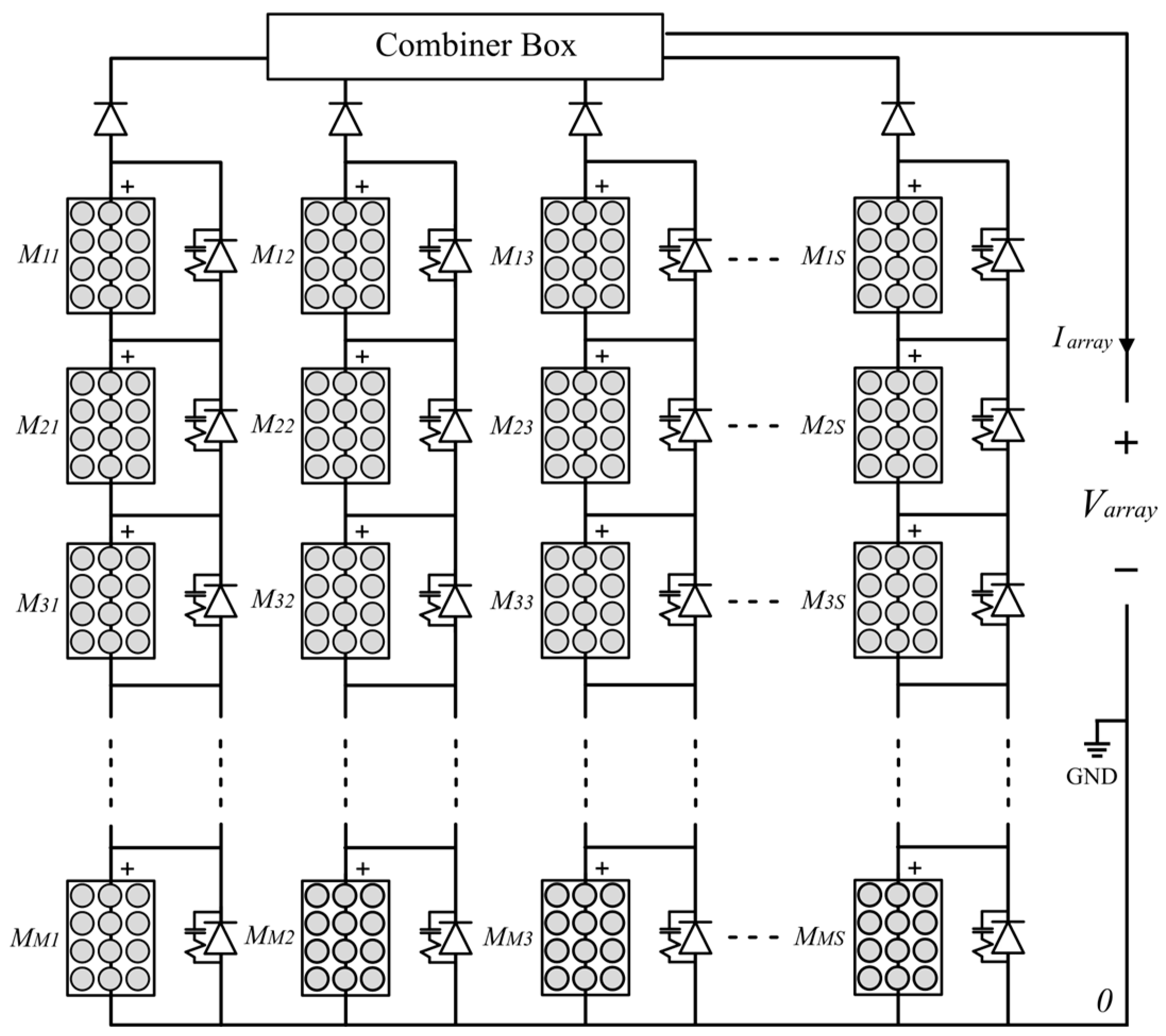
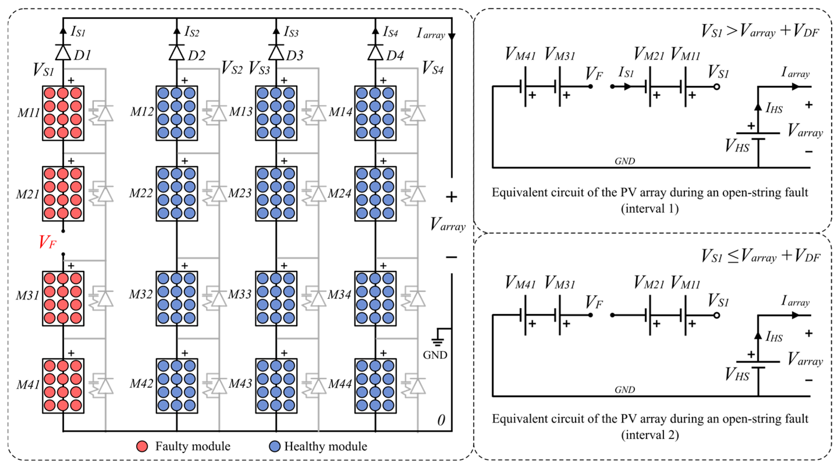
2.1. Configuration of the Considered Utility-Scale PV System

A sample of a large-scale PV array, with series modules (M) and parallel strings (S), is shown in Figure 1. The total number of parallel strings and series modules are donated as N_S and N_M, respectively. The module name was selected based on its order within the PV array. For example, M23 represents the second series module in string number 3. In an ideal-case scenario, the output current, voltage, and power are the same for each PV module, and therefore, for each array string. The combiner box is used to collect the string’s output power through a common DC rail and apply overcurrent and overvoltage protection devices.

Since the PV array is vulnerable to a variety of physical issues and electrical faults due to their exposure to harsh outdoor conditions, targeting large-sized photovoltaic systems, starting from 5 megabytes and higher, makes many of the traditional fault diagnosis methods in doubt. The large areas covered by these systems require the use of novel methods that overcome the challenges and difficulties in determining fault locations.

Referring to Figure 1, the terminal voltage and current of the PV array (V_array and I_array) are dependent on the captured solar radiation, weather conditions, model characteristics, and configuration. The type and location of a potential PV failure influence the behavior of the array’s voltage and current, as well as the faulty string. The next sections illustrate and analyze the symptoms and array performance under the most common PV array faults, aiming to understand the behavior of key elements like array current and voltage during these faults.

2.2. Definition of Fault Analysis Variables

As the terminal open-circuit voltage, short-circuit current, and maximum power of a certain PV module are reachable, the behavior of the PV array terminal variables can be evaluated and utilized as significant indicators for fault events. This section discusses the PV array fault analysis to be utilized for the fault localization approach. For this reason, the following parameters are introduced:

• Open-circuit test voltage (V_OT): The PV array voltage under an open-circuit condition.
• Short-circuit test current (I_ST): The PV array current under a short-circuit test condition.
• Maximum test power (P_MT): The PV array power under the MPPT test condition.
• String difference voltage (U_XY): The voltage difference between each of the two neighboring strings. For this test, the voltage of a PV string is measured at the positive node of the top module of the string and prior to the series blocking diode.
• Fault voltage (V_F): The resultant abnormal voltage at where the fault event occurs.
• Fault current (I_F): The resultant current flowing through the fault path.
• Fault resistance (R_F): The accumulated DC resistance of the fault path.
• Diode forward voltage drop (V_DF).

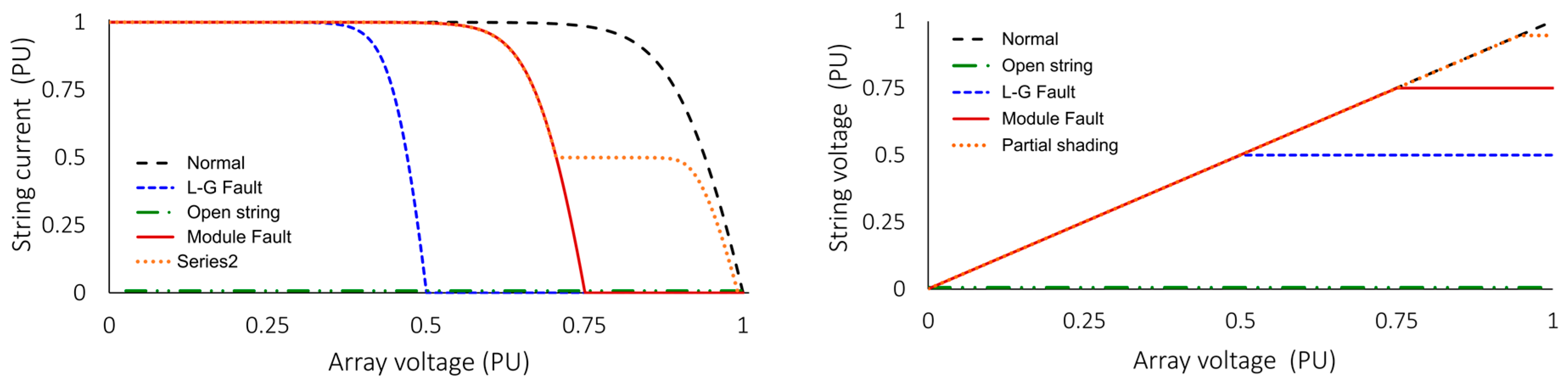
2.3. PV Array Fault Analysis

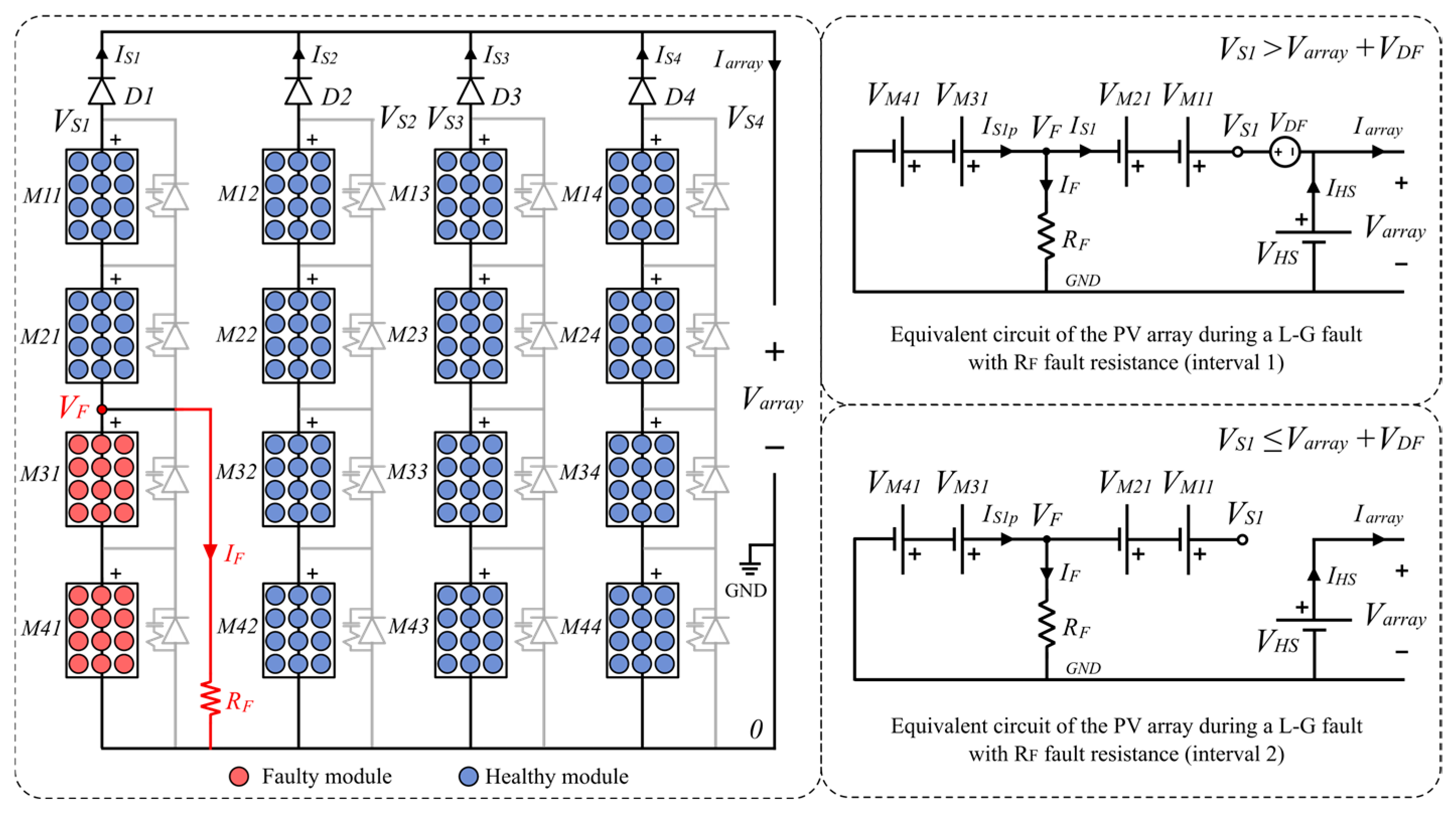
2.3.1. Line-to-Ground Fault

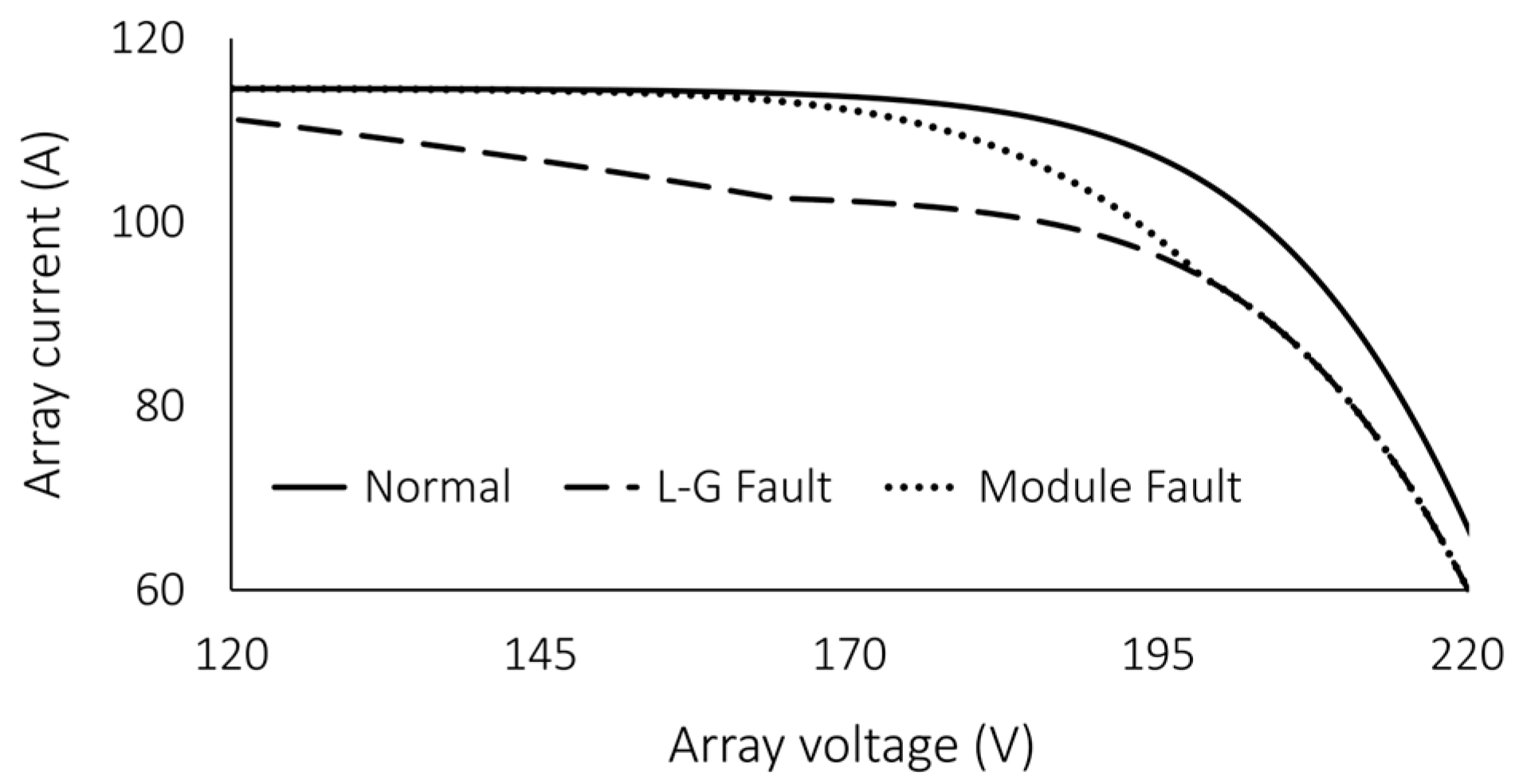
Line-to-ground faults in PV arrays are akin to short circuits occurring between ground and one or more active conductors, as shown in Figure 2. During the L–G fault between modules M31 and M41, the faulty string current will continue flowing (i.e., diode D1 is conducting) as long as the array terminal voltage is lower than V_S1.

Once the array voltage (V_array) becomes equal to or higher than the faulty string, which in this case equals the sum of voltages across the module M11, module M21 and fault resistance (R_F), the diode D1 becomes reverse biased. This event occurs due to the fact that the array voltage was building up, assuming a zero voltage initial condition, until the voltage difference between the anode and cathode of the diode D1 reached zero or a negative value, which can be formulated as follows:

$$N_H{V}_{OC}+V_F<V_{array}+V_{DF}$$

(1)

where N_H is the number of health modules. The fault resistance (R_F) has a direct impact on the faulty string behavior during L–G faults. For L–G faults with zero or low fault resistance (LR_F), the obvious symptoms to detect the fault are the reduction in array output power due to the string opening and the voltage reduction at the diode positive (anode) node. The reduction in the output power depends on the number of faulty strings, where it could be reduced due to only one faulty string or due to (N_S − 1) strings. Hence, the array output power could be reduced by 1/N_S times at least or (N_S − 1)/N_S times at most. This creates the first power sensing condition (sensing condition 1), as in Equation (2).

For L–G faults with high fault resistance (HR_F), the voltage drop across the fault path resistance can increase string terminal voltage (V_S), which maintains a forward-biased state for the series blocking diode. The obvious symptoms to detect this fault are the reduction in the array output power and the voltage at the blocking diode positive (anode) node. The HR_F L–G fault can be differentiated from the LR_F L–G fault by the reduction amount in the array output power, whereas in the case of the HR_F L–G fault, the array output power is reduced by less than 1/N_S times due to the faulty string feeding current. This creates the second power sensing condition (sensing condition 2), as stated in Equation (2). Moreover, the diode positive voltage will be higher in this case due to the high voltage drop across the fault path resistance (HR_F).

Both L–G fault case scenarios could be detected by the following conditions:

$$\left\{\begin{array}{c}sensingcondition1:P_{arrayF}\le P_{arrayN}\left(N_S-1\right)/N_S\\ sensingcondition2:P_{arrayN}\left(N_S-1\right)/N_S\le P_{arrayF}\le P_{arrayN}\end{array}\right.$$

(2)

where P_arrayN and P_arrayF are the array output power during normal and fault conditions.

2.3.2. Module Fault

An inter-string PV fault refers to a short-circuit between PV modules or array wires of varying potentials. For module faults, as shown in Figure 3, the faulty string behaves as an L–G faulty string during the time period when the blocking diode is forward biased.

Once the array voltage (V_array) becomes equal to or higher than the faulty string, which in this case equals the sum of voltages across the module M11, module M21, module M41, and the fault resistance (R_F), the diode D1 becomes reverse biased since the array voltage was building up until the voltage difference between the anode and cathode of diode D1 reached zero or a negative value. The power and voltage conditions and differentiation method for module faults (with LR_F and HR_F) are similar to those for the L–G fault type.

Since the L–G and module faults have the same symptoms, two more indicators are needed to differentiate these two fault categories from each other. First, the LR_F module fault is characterized by its impact on the blocking diode voltage, where only a single module within a faulty string will be open-circuited, meaning that the voltage across the blocking diode will be approximately V_OC. In contrast, the LR_F L–G fault leads to two or more open-circuited modules; otherwise, it becomes an LR_F module fault. Hence, during L–G fault type, the voltage across the blocking diode will be approximately mV_OC, where m is an integer number greater than 1.

Second, the HR_F module fault is characterized by its impact on the array I–V characteristic, where the array current has a detectable, consistent decay pattern, as illustrated in the next section.

2.3.3. Partial-Shading

PV systems frequently experience shading from various sources, such as clouds, trees, poles, and buildings, which can partially or fully cover PV modules. For the partial shading scenario on a single or multiple PV modules, as shown in Figure 4, the affected string behavior during constant solar radiation can be obtained based on the level and duration of shade.

For a better understanding of the affected string behavior, the module I–V characteristic under the partial shading event must be analyzed. As is well known, reduced solar radiation has a direct impact on the module’s generated current and, therefore, the output power. This impact can be modeled using a linear relationship along with the module standard test conditions (STC) characteristics, as discussed in [37]. Figure 5 shows the I–V curve for the utilized PV module under solar radiation levels. As observed from the figure, the short-circuit current changes linearly (with a constant slope), while the open-circuit voltage remains within a very narrow range (between V_OC and 0.95 V_OC). This implies that during the partial shading event, the string series blocking diode is maintained forward biased, and the faulty string continues its current contribution.

The behavior of a string during a partial shading event is shown in Figure 6, which could be broken down as follows: At the beginning of region 1 (V_array ≅ 0), the partial shading event will not show symptoms in the faulty array, meaning that the string generates the same short-circuit current as healthy strings. During region 1, the bypass diode across the faulted module will be forward biased to pass the current difference between the healthy and faulted modules; consequently, the building-up array terminal voltage will be distributed uniformly only across the health modules, as the faulted one is short-circuited by the bypass diode. During region 2, as the array voltage keeps increasing, the voltage across the healthy modules reaches near V_OC; hence, the string current starts to fall down until the point where the healthy modules’ series current matches the current of the faulty module. At this point, the bypass diode of the faulty module turns to be reverse biased, and the whole string flows the I–V characteristic of the faulty module, as demonstrated during region 3. During this region, the voltage across the faulty module takes its turn to withstand the increment in the array terminal voltage.

The partial shading, HR_F L–G, and HR_F module faults have the same symptoms as the PV array; hence, they have the same power and voltage conditions. In order to differentiate partial shading from the same category faults, one more indicator is needed, which is the array I–V curve during the MPPT operating point. During the MPPT operation, the faulty string is characterized by its curved and step-change pattern because it follows the I–V curve of the shaded module shown in Figure 5. Figure 7 illustrates the faulty string I–V curve when experiencing faults with the same power and voltage symptoms.

2.3.4. Open-Circuit Fault

An open circuit fault arises when no current flows through all solar panels within a string due to physical failures, as shown in Figure 8. All modules (and bypass diodes) are capable of passing short circuit currents under all array normal and fault conditions, except the open-string condition, as clearly seen in Figure 9 (left). Therefore, any reduction in the sort-circuit current is considered a sign of an open-string fault.

3. PV System Modeling and Considered PV Faults

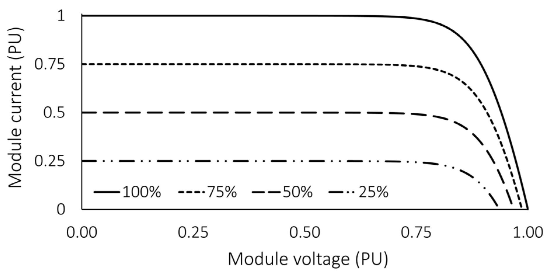
3.1. PV Panel Model and Characteristics

Solar energy is converted directly into electrical power through solar cells. Hence, the PV array consists of multiple strings connected in series and parallel configurations to achieve specific output voltage and current levels. The PV cell can be modeled as a direct-current (DC) current source connected to a shunt diode with associated diode current (I_diode), shunt resistance with associated shunt current (I_shunt), and a series resistance to carry out the generated current. As a result, the PV cell behavior can be described by [23]:

$$I_{pv}=I_{ph}-\left[I_{diode}+I_{shunt}\right]=I_{ph}-\left[I_{R0}\left(exp\left({\displaystyle \frac{V_{pv}+I{R}_s}{n{V}_T}}\right)-1\right)+{\displaystyle \frac{V_{pv}+I{R}_s}{R_{sh}}}\right]$$

(3)

where I_pv is the cell output current, I_ph is the photo-current controlled by light intensity I_R0 is the reverse saturation current and V_pv is the voltage generated by the PV cell. R_s and R_sh are the solar cell series resistance and shunt resistance; respectively, whereas n is the cell ideality factor.

The transient model of the PV solar cell shows that the resulted values of voltage and current depend on both radiation and temperature, where the ambient temperature plays a pivotal role in quantifying the thermal voltage and formulated resistors. Therefore, with any changes in temperature and radiation, the form of the relationship between current and voltage, as well as power and voltage, varies. Due to this behavior, the well-known current–voltage (I–V) and power–voltage (P–V) solar cell characteristics arose [38].

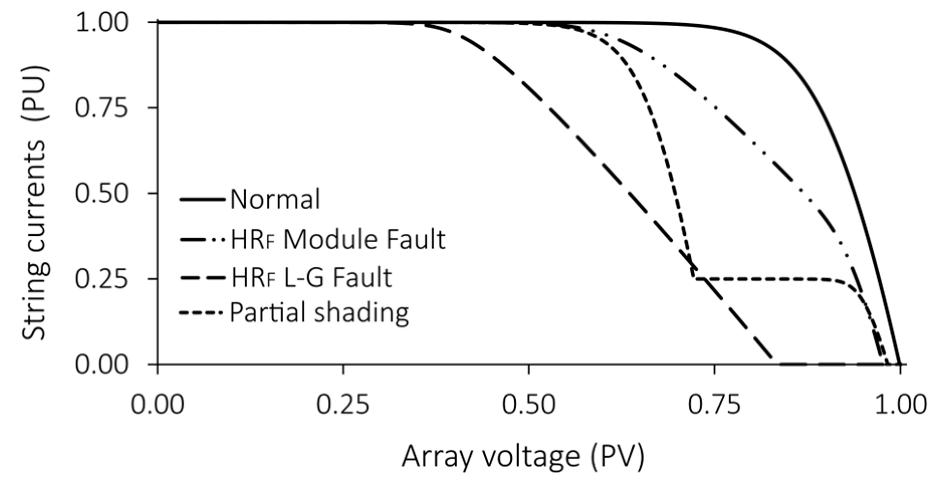
3.2. Considered PV Array Faults

This study introduces a novel technique for precisely identifying and locating various types of faults, such as line-to-ground, open-circuit, inter-string DC faults, and partial shading faults, within a large-scale PV array down to the module level. The above-mentioned faults are the most common faults in PV arrays; therefore, this study focuses on these types of array failures.

In order to show the impact of the considered faults on the PV array performance, Figure 9 illustrates the effect of the above-mentioned faults on the whole system current and power versus the array voltage. This figure was extracted from a 4 by 4 PV array to illustrate the fault impact clearly. All quantities were converted to per-unit values in order to generalize the impact demonstration. Also, the effect of faults on the faulty string’s current and voltage is shown in Figure 10.

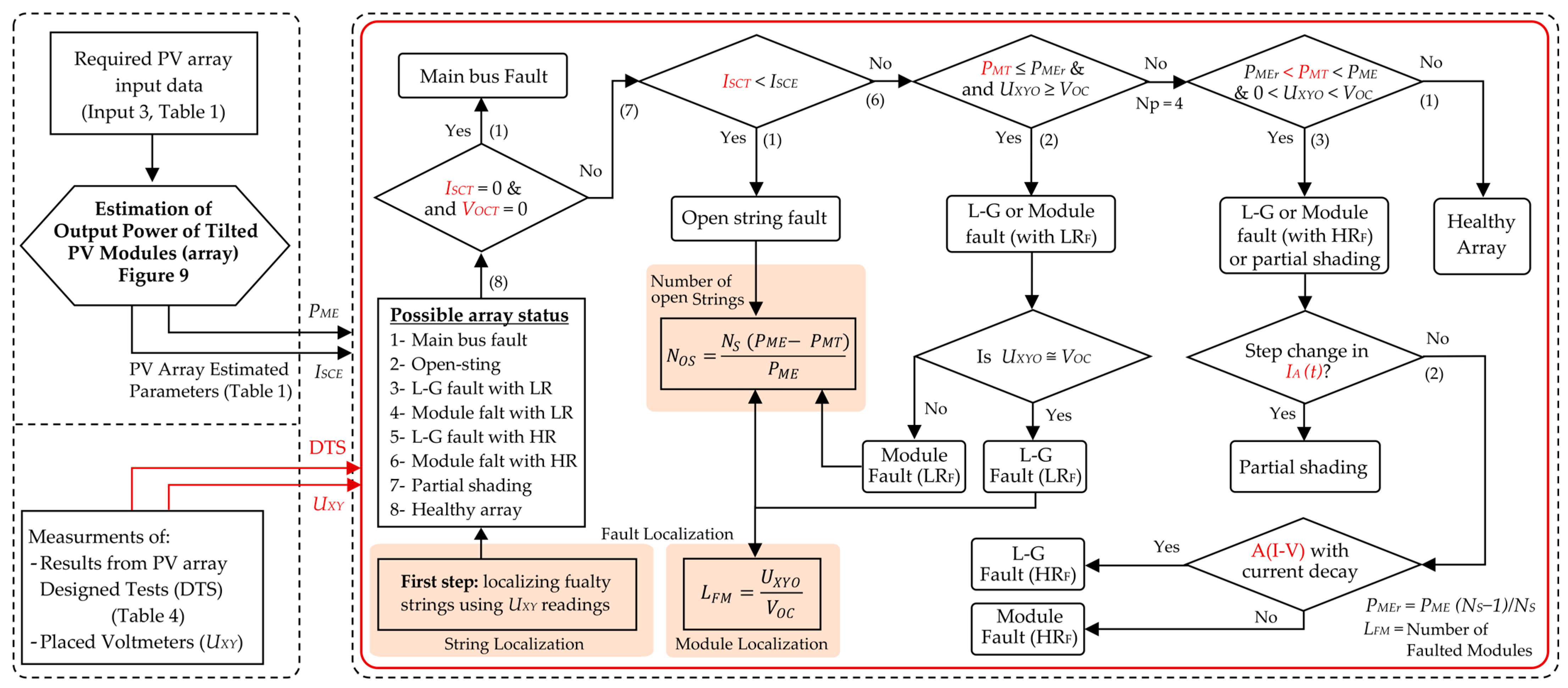
4. Fault Detection and Localization Approach

The methodology proposed in this study for fault detection, classification, and localization relies mainly on three crucial indicators: (1) strategic placement of a limited number of differential voltage sensors; (2) execution of specifically specified tests; and (3) precise calculation of the photovoltaic module’s power output. This section discusses the first two indicators, while the procedure for estimating the PV array output power is discussed in the next section.

4.1. Placing of Strings-Difference Voltage Sensors

As the PV array consists of identical parallel strings, the current and voltage across all strings must be similar during normal operating conditions. In the case of a module or string fault event, only the faulted string shows noticeable changes in terms of voltage and/or current reduction, which is utilized for fault diagnosis. In some fault cases, like L–G faults, these symptoms are used for fault localization. Hence, it is feasible to regard the remaining health strings as reference branches, which can be compared with defective strings to identify the occurrence of faults, in addition to other detecting indicators.

Consequently, the technique initially relies on identifying the faulty string by measuring the voltage difference between the two neighboring strings. Once the faulty string is specified, the resultant voltage difference associated with each of the two strings is used, along with the other detection methods, to obtain the fault type and location within that string. In order to involve all of the string’s modules in this measurement step, the voltmeters are placed on top of each string, followed by the series-connected diodes, as shown in Figure 11. The voltage difference is noted as (U_XY), where X and Y represent the negative and positive terminals of the voltmeter, respectively. It is worth mentioning that the string voltage difference can be measured during open-circuited array (U_XYO), short-circuited array (U_XYS), and maximum power operation (U_XYM).

4.2. Selectively Designed Tests

Since the PV array can experience different types of DC faults, more technical indicators must be involved. The short-circuit test and the open-circuit test are the most commonly utilized tests. In addition, this study considers more tests, such as capacitor and MPPT load tests, in order to evaluate the transient behavior of the PV array terminal voltage and current. The transient behavior is very essential in differentiating among different fault types that cause similar symptoms during open-circuit and short-circuit type tests, for example, L–G and module faults. For a better demonstration of the designed qualitative tests, all test types, collected parameters, and symbols are summarized in

Table 2. Required tests for PV fault detection and classification procedures.

Test Type	Description	Collected Parameters	Symbol
Short-circuit test	Measuring the array actual current under a PV array short-circuit (or very small resistance) condition	Array short-circuit test current	ISCT
Open-circuit test	Measuring the array’s actual terminal voltage under an open-circuit condition	Array open-circuit test voltage	VOCT
Variable voltage test	Obtaining the array’s I–V curve and transient behavior of actual terminal power and current, with utilizing a variable DC voltage source. At the voltage magnitude associated with the array’s maximum power point, power, voltage, and current can also be collected	Array I–V curve Array transient current Array transient terminal voltage MPPT transient power	A(I–V) IA (t) VA (t) PMT (t)

.

4.3. Faults Classification

The proposed methodology in this study is designed to follow the logical sequence fault detection process. In other words, the initial step in identifying the cause of unusual array behavior is assigning the faulty string by measuring the voltage difference between each of the two neighboring strings. Second, the rejection method is utilized to sort out among different array possible statuses based on the PV array signs discussed in Section 2. The possible array status considered in this study includes a heathy array, main bus fault, open-string fault, L–G fault with LR_F, L–G fault with HR_F, module fault with LR_F, module fault with HR_F, and module partial shading.

Each fault within the array strings is characterized by special impact behaviors, which, fortunately, can be distinguished from other faults.

Table 3. Summary of sensing conditions to diagnose PV fault events.

Array Status	Conditions	Explanation and Classification
Health array	PMT = PME 1 ISCT = ISCE 2	The essential test parameters to detect array faults are the terminal current and voltage (or power). If these two parameters are as expected, all strings are not experiencing any type of fault
Fault at main bus	ISCT = 0 VOCT = 0	Based on the above condition, if the array current and voltage are both not existing, all strings are experiencing an L–G fault. This scenario is possible when the main array bus (or combiner box) is under fault
Open-string fault	ISCT < ISCE	All modules (and bypass diodes) are capable of passing the short-circuit current. This is true under all array conditions, except the open-string condition. Therefore, any reduction in the sort-circuit current is considered a sign of an open-string fault
L–G fault with LRF	PMT ≤ PMEr 3 UXYO ≥ 2VOC	During HRF L–G faults, the series diode of the faulty string will become reverse biased; hence, the array MPPT power will be less than the expected power by NFS/NS, where NFS is the number of faulty strings. The voltage difference between the healthy and faulty strings roughly equals a multiple of the open-circuit voltage (mVOC), based on the fault location. The index m is an integer number greater than 1, where (m = 1) represents a L–G fault across the bottom module, meaning a module fault type
L–G fault with HRF	PMEr ≤ PMT ≤ PME 0 < UXYO < VOC A(I–V) with a current decay	During HRF L–G faults, the faulty string series diode will remain forward biased. So, the array MPPT power lies between PME and PMEr. The voltage difference between the healthy and faulty strings will not exceed the open-circuit voltage under any array operating point. The HRF L–G fault can be differentiated from module faults and partial shading by analyzing the array I–V curve, as discussed in Section 3
Module fault with LRF	PMT ≤ PMEr UXYO ≈ VOC	The first condition here is similar to the first condition of the L–G fault with LRF. The module fault here can be differentiated from L–G with LRF faults by the string voltage difference, which approximately equals the open-circuit voltage, where only one module within a string will be short-circuited, as discussed in Section 3.
Module fault with HRF	PMT < PME 0 < UXYO < VOC A(I–V) with a special pattern	The first two conditions here are similar to the first two conditions of the L–G fault with HR. The module fault here can be differentiated from L–G with HR faults by analyzing the array I–V curve, as discussed in Section
Module partial shading	PMT < PME 0 < UXYO < VOC A(I–V) with a current step	The first two conditions here are similar to the first two conditions of the L–G fault with HR. The module partial shading can be differentiated from L–G and module faults with HR by analyzing the array I–V curve, as discussed in Section 3

¹ P_ME is the estimated PV array maximum power; ² I_SCE is the estimated PV array short-circuit current; ³ P_MEr is the least reduction in the expected MPPT power and equals to P_ME (N_S − 1)/N_S.

lists the sensing conditions to classify and locate the considered PV array faults.

From the knowledge of the maximum PV array output power, via the estimation process, the number of open-circuited strings (N_OS) due to faults can be determined. This step can be done by obtaining the reduction in the measured array power with respect to the expected array power and multiplying it by the number of strings (N_S) as follows:

$$N_{OS}={\displaystyle \frac{N_S\left(P_{ME}-P_{MT}\right)}{P_{ME}}}$$

(4)

In addition, for the LR_F L–G fault, the exact fault location (L_FM) can be found by dividing the difference voltage between healthy and faulty strings during the open-circuit condition (U_XYO) by the module open-circuit voltage (V_OC). The rejection process, to classify the possible fault event, is illustrated by a flow chart as shown in Figure 12.

5. Estimation of PV Power Based on Captured Solar Irradiance Energy

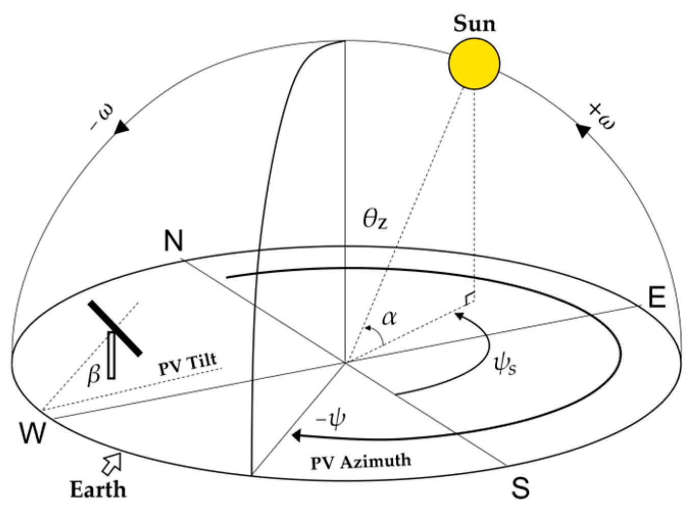
5.1. Estimation of the Solar Radiation Energy

As is commonly known, photovoltaic (PV) panels are utilized to convert solar radiation energy into electrical power. Therefore, the initial stage in determining the PV output power is to have knowledge of the solar energy received in a certain region and captured by the constructed PV panels. Several studies have investigated various mathematical models to quantify the captured solar energy [39,40]. However, the selection of a model is contingent upon its simplicity and fitting accuracy. Based on intensive mathematical analysis, including accuracy investigation tests such as the normalized root mean square error (N_RMSE), some solar irradiation energy models can be carefully nominated.

This research utilizes a solar radiation model, which considers the above-mentioned modeling concerns, to compute the quantity of solar energy that would be received for each possible design of a PV system [41]. The selection procedure was driven by the required number of input parameters and the level of precision of the utilized model.

The arrival of solar energy on the globe follows discernible patterns. These patterns may be classified based on their energy content and atmospheric aspects. The primary constituent carries the bulk of the radiation energy and focuses a beam of light onto the surface of the PV panel. The secondary component of solar energy consists of two subcomponents: albedo radiation, which refers to radiation reflected off the ground, and scattered radiation, which refers to radiation reflected by other objects.

Instead of calculating the overall radiation power, the potential solar energy is determined by evaluating the intensity of sunlight. Based on the information given before, the time-varying solar energy received at a slanted surface (I_Rt) can be expressed by [42]:

$$I_{Rt}\left(T\right)=I_0\left(T\right)\overline{K_T}\left\{\left(1-K\right)C_R+\left(K\right)F_{RS}+{\mu }_g{F}_{Rg}\right\}$$

(5)

It is clearly seen from the above equation that the total solar irradiance energy depends on different terms, as follows:

• The direct radiation beam, which is represented by the solar radiation energy on a flat surface (I₀).
• The surface orientation is where the surface tilt and azimuth angles are considered. The impact of different surface orientations is included in the orientation coefficient (C_R). This factor varies from 0 to 1, where C_R = 1 when the collector surface is flat to the ground.
• The radiation view factor between the sky and the collector F_RS, and it is included to measure how far the surface is facing the sky. This factor varies from 0.5 to 1, where its lowest value occurs when the tilt angle of the collector is 90°.
• The level of collected scattered radiation, where it can be included via the radiation view factor between the ground and collector F_Rg. This factor principally measures how the collecting surface is facing the ground. It varies from 0 to 0.5, where its lowest value occurs when the collector surface is flat to the ground.
• The sky condition index (K_T), which concerns about the weather condition. This index varies from 0 to 1, where its highest value occurs in the case of a clear sky. The constant K is dependent on the sky condition index and can be obtained as in Equation (6).
• The capability of the ground to reflect the sun’s radiation, which can be accounted via the ground reflectance factor μ_g. This factor varies from 0 to 1, where its lowest value occurs in the absence of scattered radiation. Normally, this factor is set at 0.6 during the winter season and 0.2 for the rest of the year.

$$\left\{\begin{array}{c}K=1-0.09\overline{K_T}\overline{K_T}\le 0.22\\ \\ K=0.95-0.16\overline{K_T}+4.3{\left(\overline{K_T}\right)}^2-16.6{\left(\overline{K_T}\right)}^3+12.3{\left(\overline{K_T}\right)}^{4}0.22\le \overline{K_T}\le 0.8\\ \\ K=0.1136\overline{K_T}\ge 0.8\end{array}\right.$$

(6)

The time-variant solar energy captured by a flat surface (I₀) is totally dependent on the air mass (AM), which is the straight atmospheric passage between the sun and a point of interest. Generally speaking, the maximal irradiance energy is obtained when the sun radiation beam is perpendicular to a point at sea level, or AM1. As a result, reduced solar energy is produced by solar radiation beams that are less than 90° since their air mass is greater than unity. Based on the Aden B. M. and Marjorie Pettit M. solar radiation model [42], the time-variant solar energy captured by a flat surface (I₀) can be expressed as:

$$I_0\left(T\right)=1377\times {\left(0.7\right)}^{{AM\left(T\right)}^{0.678}}\left(\mathrm{W}/{\mathrm{m}}^2\right)$$

(7)

The solar constant 1377 represents the average solar power in the earth’s atmosphere, while the factors 0.7 and 0.678 represent the direct and scattered radiation, respectively. The air mass is proportional to the secant of the altitude angle (α), which is the angle between the horizontal axis and the direct sunlight beams, as clearly shown in Figure 13. Therefore, the air mass (AM) can be expressed as a function of the altitude angle (α), which is a function of the latitude of the site location, the declination angle (δ), and the solar hour angle (ω). These angles are well explained and derived in [41,42].

Moreover, to consider the PV panel’s orientation in the estimation process, the correlation factor (C_R), which represents the surface azimuth and tilt angles, is included. The correlation factor C_R is well discussed and expressed in [41], while the radiation view factors (F_RS and F_Rg) can be expressed as functions of module tilt angle (β) as follows:

$$\left[F_{RS},F_{Rg}\right]=0.5\left[1\pm cos\left(\beta \right)\right]$$

(8)

5.2. Estimation of the PV Output Power

It is widely known that PV panels cannot fully convert all of the solar energy they absorb into electricity. This is due to factors such as PV panel efficiency (n_p), temperature-to-power coefficient (β_P), and power loss (P_loss) in energy conversion equipment, which significantly reduce the amount of power generated by the PV panels [43,44]. Hence, considering these aspects, the generated PV output power (P_PV) shall be expressed as:

$$P_{PV}\left(T\right)=I_{Rt}\left(T\right)\times \left({\eta }_p{N}_p{A}_p{\beta }_P\right)-P_{loss}\left(\mathrm{kW}\right)$$

(9)

where N_p and A_p are the number and area of the PV panels, respectively. The process of estimating the PV output power starts first with collecting the necessary input parameters listed in

Table 4. Required input data for the PV power estimation process.

Data Type	Classification	Name	Parameters
Input data (collected)	Location and time information	Input 1	- Latitude, longitude, and day number 1 - Time zone (with respect to GMT 2) - Longitude of noontime (daily basis)
	PV module specifications	Input 2	- Module tilt and azimuth angles - Power, voltage, and current thermal coefficients - Module reference efficiency at STC 3 temperature - Module geometry (surface area)
	PV system specifications	Input 3	- Modules count - System capacity and array configuration - Open-circuit voltage (VOC) and short-circuit current (ISC) at STC - MPPT voltage (Vm) and MPPT current (Im) at STC - Power loss in cables and power converters
Input data (measured)	Weather factors	Input 4	- Ambient temperature and sky condition index (KT)
Output data (Estimated)	PV array outputs	Output 1	- Estimated PV array MPPT 4 power (PME) 5 - Estimated PV array short-circuit current (ISCE) 5

¹ Number of the day considering the Gregorian calendar; ² Greenwich Mean Time; ³ standard test conditions; ⁴ maximum point power tracking; ⁵ under all possible solar radiation and module orientation case-scenarios.

. Second, the mathematical estimation model is applied. Third, the PV output power is obtained by considering the number, area, and efficiency of the PV panels, along with the ambient temperature and system power loss, as formulated in Equation (9).

The flow chart in Figure 14 visually illustrates the process for PV output power estimation. Also, the flowchart shows a comparative analysis to validate the estimation model, where the extracted results are compared to actual field data collected from a particular PV system, as discussed in the next section. A 5% mismatch is considered the threshold computational error to pass the estimation model results.

In order to show samples of the model outcomes, solar irradiance energy for different days was estimated, as shown in Figure 15. The days considered in this part were carefully selected to cover different seasons throughout the year. It is worth mentioning that this estimation process was conducted for the region of Riyadh, Saudi Arabia, with 24.7136° N and 46.6753° E latitude and longitude, respectively. The ambient temperature was fixed at 35° Celsius, whereas module orientation has three options, as listed in

Table 5. Different PV module orientation for estimation model demonstration.

	Orientation 1	Orientation 2	Orientation 3
Tilt angle	0 degree	24 degree	24 degree
Azimuth angle	0 degree	0 degree	45 degree

.

In addition to the maximum power, the commonly used PV module parameters for DC fault diagnosis are the open-circuit voltage (V_OC) and short-circuit current (I_SC). Therefore, it is essential to obtain them in the estimation process. The V_OC is mainly dependent on the internal module specification, such as the number and configuration of internal semiconductor solar cells, which makes the V_OC remain within a narrow range (1.0 to 0.95 PU) under any operating point. The expected short-circuit current (I_SCE) varies based on the solar radiation intensity with a constant slope-linear relationship, as illustrated in Figure 5. Consequently, I_SCE can be expressed as a function of solar radiation, as follows:

$$I_{SCE}=I_{SC\_STC}\times Max\left(I_{Rt}\left(T\right)\right)/1000$$

(10)

where 1000 and I_{SC_STC} are, respectively, the solar radiation power and module short-circuit current at STC.

6. Case Study Results and Discussion

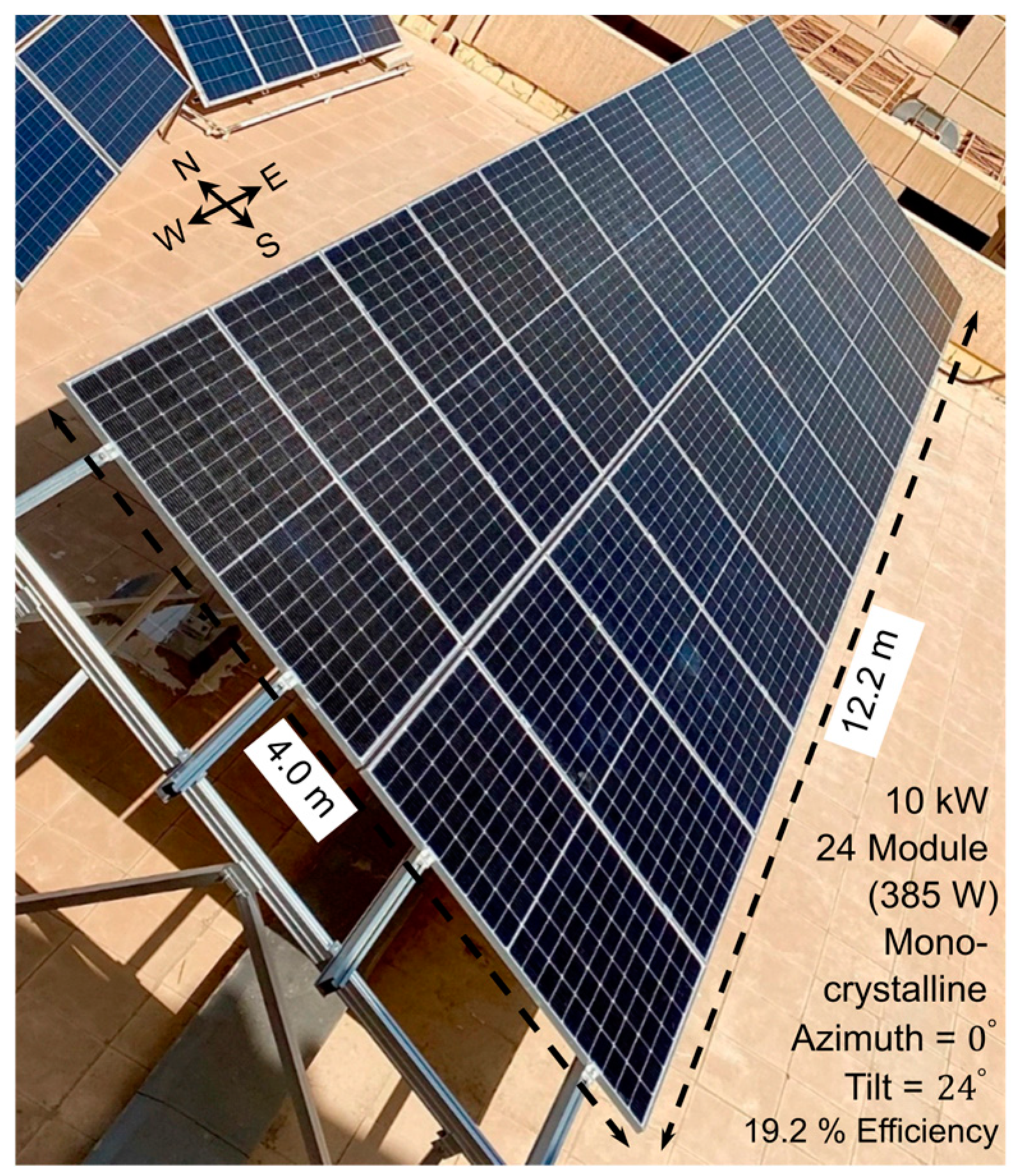
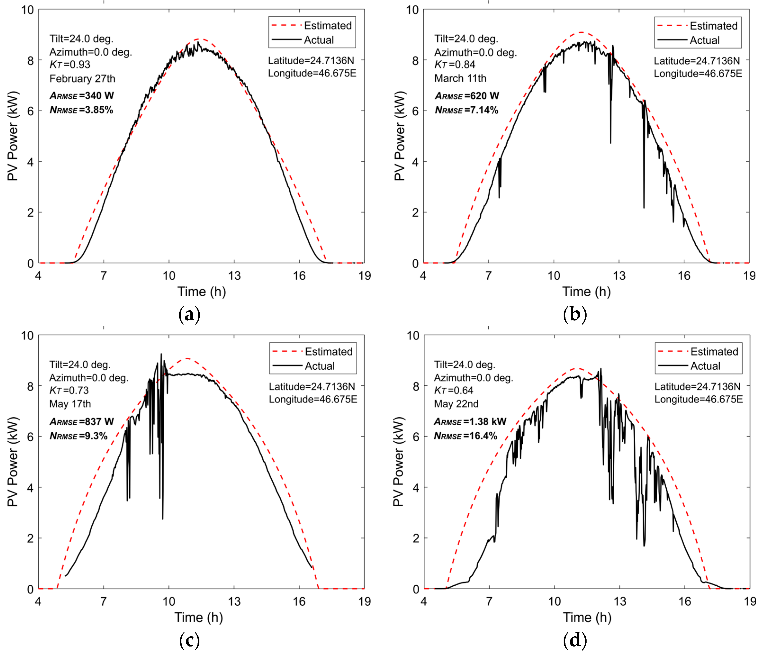
6.1. Validation of the PV Power Estimation Model

The utilized model for estimating the generated PV power was validated using actual data from a 10 kW laboratory PV system, as depicted in Figure 16. The validation process involved several steps. First, real power data from the considered PV system was collected. Second, the required PV system data, as in Table 4, and PV module parameters, listed in

Table 6. PV Module parameters (JA solar-Monocrystalline MBB).

Parameter	Value	Parameter	Value
Maximum power (Pmax)	385 W	Module efficiency	19.2%
Open-circuit voltage (VOC)	39.82 V	Maximum power voltage (Vm)	32.65 V
Short-circuit current (ISC)	12.52 A	Maximum power current (Im)	11.79 A
Temperature coefficient of ISC (βI)	+0.044%/°C	Temperature coefficient of VOC (βV)	−0.272%/°C
Temperature coefficient of Pmax (βP)	22120.350%/°C	STC	1000 W/m2 and 25 °C
Location coordinators	(24.7136° N, 46.6753° E)	Module orientation	Tilt angle: 24°, azimuth: 0°
Module size	2.10 m × 1.05 m	Ambient temperature	35 °C

, were gathered. Third, the estimated PV output power was calculated and calibrated for accuracy. Finally, the model’s correctness was assessed using a fit test error, specifically the actual root-mean-square error (A_RMSE) and the normalized root mean square error (N_RMSE) [42], where both can be formulated as follows:

$$N_{RMSE}={\displaystyle \frac{A_{RMSE}}{Maximumof\left(P_{PVA}\right)}}={\displaystyle \frac{\sqrt{{\sum }_{i=1}^n{\left(P_{PVA,i}-P_{PVE,i}\right)}^2/n}}{Maximumof\left(P_{PVA}\right)}}$$

(11)

where P_PVA,i and P_PVE,i are the ith order of the actual and estimated PV power; respectively, and n is the total number of readings samples.

The PV system’s output power was measured and compared to the estimated PV power at fixed tilt and azimuth angles for various weather conditions, such as sunny, partly cloudy, and cloudy days, as shown in Figure 17. The figure also shows the results of the A_RMSE and N_RMSE accuracy test indices.

The comparison revealed that during sunny days, with a clear sky index (K_T) of 0.90 or higher, the alignment between the estimated and actual PV power values was evident in Figure 17a. This alignment was characterized by smaller errors and correspondingly lower N_RMSE values, indicating the model’s high accuracy. However, on partly cloudy and cloudy days, with K_T values below 0.90, the estimated PV power deviated more from the actual values due to increased solar irradiance variability. Consequently, it is essential to highlight that the model validation process focused solely on sunny days, on which the N_RMSE is considerable. Thus, the results show the feasibility of the estimation model and, thereby, affirm the utility of the model in PV system fault localization.

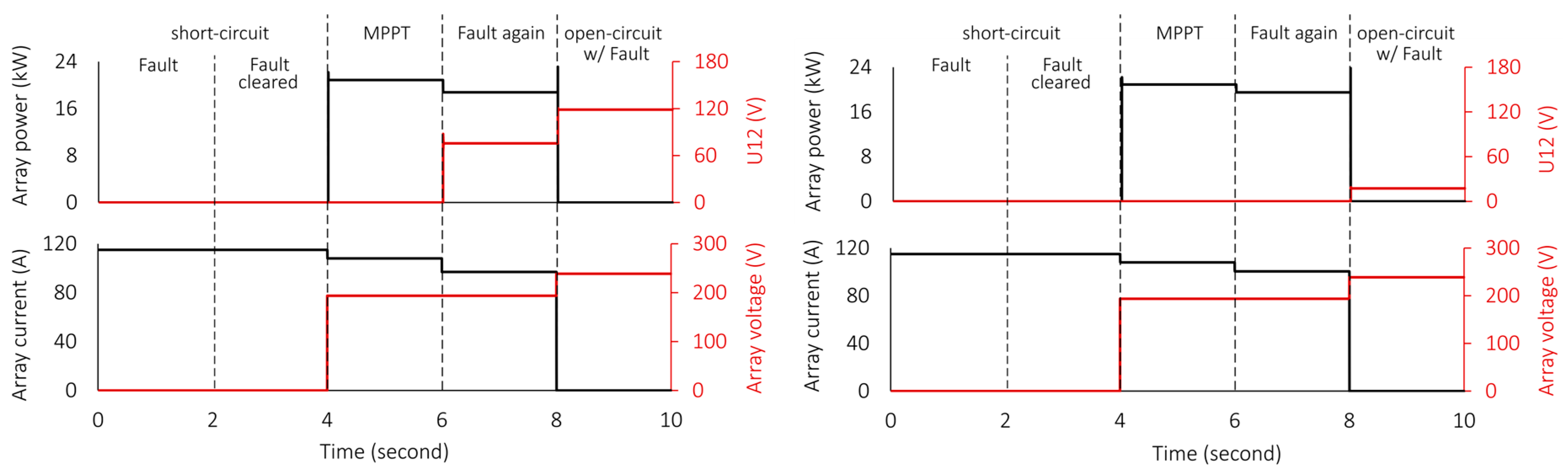
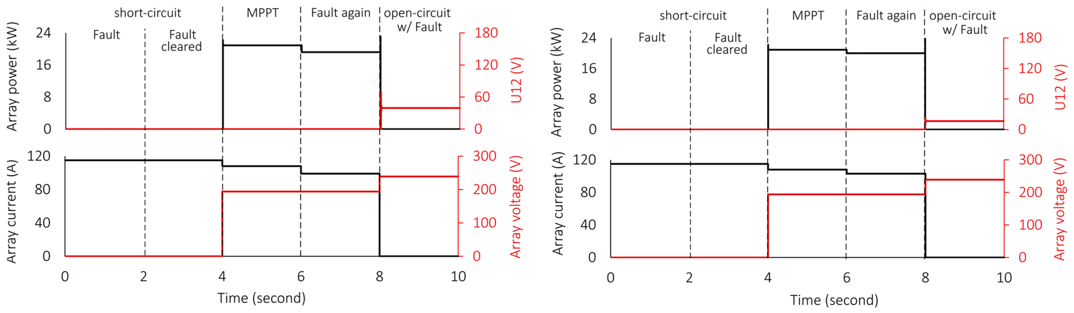
6.2. Validation of the Proposed Fault Detection and Classification Methodology

In order to validate the feasibility of the proposed method for PV array fault detection, classification, and localization, a 6 × 10 PV array was considered, with the PV module parameters listed in Table 6. Additionally, five differential voltage sensors were placed based on the proposed method, as illustrated in Figure 11. During the fault detection process, the PV array was solely treated without the existence of DC–DC and DC–AC power converters in order to measure the intended DC quantities mentioned in Table 2 and to avoid the mismatch in MPPT test procedures.

The fault detection process was conducted for fixed solar radiation to be compared with the array measurements. For this purpose, the estimated solar radiation energy and PV MPPT power for the considered PV modules were obtained. The noontime for September 15th (with 912 W/m² of solar power), as demonstrated in Figure 15, was used for this estimation step. The resultant estimated MPPT power (P_ME) was found to be 21.04 kW. Consequently, from Equation (10), the I_SCE, for 10 strings, is 114.18 A.

In this section, different PV fault case scenarios were conducted to investigate the fault detection and classification abilities of the proposed method.

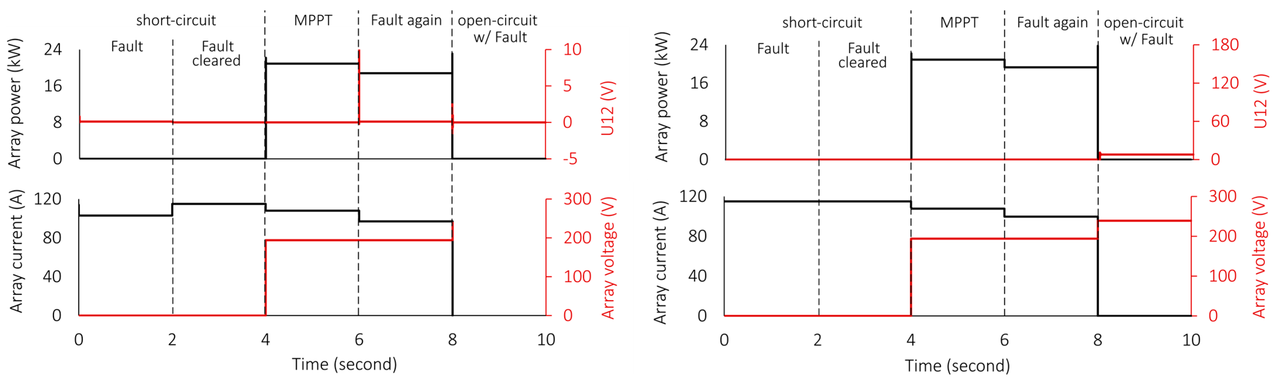
6.2.1. Line-to-Ground and Inter-String Module Faults

The line-to-ground fault was introduced to the PV array by connecting the junction cable, which links two cascaded modules within the same string, and the ground, as shown in Figure 2. The inter-string module fault was conducted by linking the positive and negative terminals of the module, as shown in Figure 3. Both faults can be conducted through an electrical wire with a variable resistor in order to simulate different fault scenarios. In this part, the L–G fault was conducted between modules M31 and M41, while the module fault was conducted for M31. The fault path for both cases was set at several resistor values, as listed in Table 7. In order to detect and classify the introduced fault, the voltage difference and the required designed tests’ readings are collected, as shown in Figure 18 and Figure 19.

It is concluded that the obtained test results are consistent with the proposed method and the classification procedure illustrated in Figure 12. After detecting the faulty string through the voltage difference sensors, the array maximum power, where the array terminal voltage is near the open-circuit voltage, is considered the first indicator of the internal-string fault type. Figure 18 (left) shows that when LR_F L–G fault is applied, the array power is dropped from 20.91 kW to 18.86 kW, which exactly equals the least reduction in the expected MPPT power (P_MEr), meaning that there is one open-circuited parallel string. In contrast, when the power dropped to a value between P_MEr and P_ME, as in Figure 18 (right), this fault is considered an HR_F L–G fault.

The above-mentioned conclusions can also be applied to the module fault results, illustrated in Figure 19. Moreover, the readings of the voltage difference between string 1 and string 2 during the open-circuit time period (U_12O) contribute to differentiating the LR_F L–G fault from the module ones. As discussed in this study, the difference voltage equals the V_OC. As shown in Figure 19 (left), this fault is considered an LR_F module fault; otherwise, it is an LR_F L–G fault. In addition, to differentiate between the HR_F L–G and HR_F module faults, the I–V array curve, as shown in Figure 20, is analyzed. At the maximum power region of the I–V curve, it is obvious that the curve during the L–G fault has a consistent ramp down, which distinguishes this type of fault, as discussed in Section 2. Other array parameters during the fault detection procedures are listed in Table 7.

6.2.2. Open-String Fault

The open-circuit fault was introduced to the PV array by disconnecting one end of the junction cable, linking two cascaded modules within the same string, as demonstrated in Figure 8. In this part, the open-circuit fault was conducted between modules M31 and M41. The voltage difference and required readings from the designed detecting tests are collected, as shown in Figure 21 (left). As discussed in Section 2, the obvious sign of an open-circuit fault is the reduction in the array short-circuit current, as clearly seen in Figure 21 (left). When the fault is applied, the array power is dropped from 20.91 kW to 18.85 kW, which exactly equals the least reduction in the expected MPPT power (P_MEr), meaning that there is one open-circuited parallel string. Other array parameters during the fault detection procedures are listed in Table 7.

6.2.3. Partial Shading

Partial shading was introduced to the PV array by reducing the amount of received solar radiation to certain PV modules, as demonstrated in Figure 4. In this part, the partial shading was applied to module M31. The voltage difference and required readings from the designed detecting tests are collected, as shown in Figure 21 (right). As discussed in Section 2, as the array power dropped to a value between P_MEr and P_ME, as in Figure 21 (right), and the difference voltage (U_12O) is way less than V_OC, this event is considered a partial shading case.

In addition, to differentiate between the partial shading and HR_F faults, the I–V array curve, as shown in Figure 22, is analyzed. At the maximum power region of the I–V curve, it is obvious that the curve during a partial shading event has a sharp step-change, similar to the normal operation I–V curve with reduced solar radiation. Other array parameters during the fault detection procedures are listed in Table 7.

Table 7. Summary of the conducted tests results.

Fault Type			RF (Ω)	U12O (V)	PMT (kW)	VOCT (V)	ISCT (A)	NOS	I–V Curve
Combiner box			NA	0	0	0	0	NA	NA
L–G	w/LRF		0	118.6	18.86	236.8	114.2	1	NA
			4	72.95	18.89	236.8	114.2	1	NA
	w/HRF		8	28.72	19.36	236.8	114.2	0	Figure 20
			10	17.44	19.58	236.8	114.2	0
Module	w/LRF		0	39.58	18.86	236.8	114.2	1	NA
			0.1	39.02	18.88	236.8	114.2	1	NA
	w/HRF		8	1.814	19.59	236.8	114.2	0	Figure 20
			10	1.013	19.72	236.8	114.2	0
Open-string			NA	0	18.86	236.8	102.7	1	NA
Partial shading		50%	NA	1.306	20.30	236.8	114.2	0	Figure 22
		25%	NA	2.617	19.94	236.8	114.2	0
Healthy			NA	0	20.91	236.8	114.2	0	NA

Table 7. Summary of the conducted tests results.

Fault Type			RF (Ω)	U12O (V)	PMT (kW)	VOCT (V)	ISCT (A)	NOS	I–V Curve
Combiner box			NA	0	0	0	0	NA	NA
L–G	w/LRF		0	118.6	18.86	236.8	114.2	1	NA
			4	72.95	18.89	236.8	114.2	1	NA
	w/HRF		8	28.72	19.36	236.8	114.2	0	Figure 20
			10	17.44	19.58	236.8	114.2	0
Module	w/LRF		0	39.58	18.86	236.8	114.2	1	NA
			0.1	39.02	18.88	236.8	114.2	1	NA
	w/HRF		8	1.814	19.59	236.8	114.2	0	Figure 20
			10	1.013	19.72	236.8	114.2	0
Open-string			NA	0	18.86	236.8	102.7	1	NA
Partial shading		50%	NA	1.306	20.30	236.8	114.2	0	Figure 22
		25%	NA	2.617	19.94	236.8	114.2	0
Healthy			NA	0	20.91	236.8	114.2	0	NA

The number of open-circuited strings (N_OS), shown in Table 7, can be obtained by Equation (4), while the location of faulty strings can be assigned with the help of the differential voltage sensors. In addition, the exact fault location can be determined for the L–G fault with zero fault resistance by dividing the resultant difference voltage by the module open-circuit voltage (V_OC). From Table 7, the location of this fault is after the third module (M13) as a result of dividing 118.6 V by 39.82 V.

It is concluded from the investigation process that the proposed approach has the ability to detect, classify, and localize the considered PV array faults with a reduced number of voltage sensors and power switches. In addition, the integration of PV output power estimation into the proposed fault detection method contributes to the further elimination of reference modules, which require power wires and routine cleaning and calibration. Also, compared to deep-learning and data collection-based methods, the proposed approach minimizes the expenses of the training engines and data storage systems.

Table 8. Comparison with other existing voltage sensor-based methods for a 10 × 10 PV array.

Method	Number of Components			Detects HRF 1 Fault?	Detects LRF 2 Fault?	Component to Module Ratio	Reference Module?	Cost	Module Level
	Voltage Sensors	Switches	Diodes
[45]	90	0	0	Yes	Yes	90%	Yes	Very high	Yes
[23]	1	50	0	Yes	Yes	51%	Yes	High	Yes
[46]	50	0	0	Yes	Yes	50%	Yes	Very high	Yes
[7]	45	0	0	Yes	Yes	45%	Yes	High	Yes
[47]	45	0	0	Yes	Yes	45%	Yes	High	Yes
[22]	3	0	39	Yes	Yes	42%	Yes	Medium	Yes
[48]	20	0	0	No	Yes	20%	Yes	Medium	No
Proposed	5	0	0	Yes	Yes	5%	No	Low	Yes

¹ High resistance faults; ² low resistance faults.

compares different existing voltage sensor-based methods for a 10 × 10 PV array. From the comparison, it is obvious that this study contributes to minimizing the required equipment for PV fault detection and classification and, therefore, the total cost, while maintaining accuracy, simplicity, and reliability.

7. Conclusions

This study introduced an innovative approach to diagnose and pinpoint many sorts of PV faults, including line-to-ground, line-to-line, inter-string, open-circuit, and partial shading events, for utility-scale PV systems, down to the module level. The study relied primarily on three key indicators: an accurate computation of the PV array’s output power and current, strategic positioning of a limited number of voltage sensors, and the implementation of carefully prescribed tests. By estimating the power of the PV array and strategically placing voltage sensors, the time and equipment needed for problem detection and diagnostics can be minimized. The viability of the suggested approach was examined using actual field data and the PSCAD simulation platform under various weather conditions and array defects. The findings obtained indicated that the proposed method effectively identifies, categorizes, and localizes faults using a number of voltage sensors, which corresponds to half of the string count (N_S/2). Compared to existing approaches with similar methods, the contribution of this study is really obvious, where the cost and certainty of the proposed fault diagnosis system were improved while accuracy and simplicity were maintained. It is recommended to apply the proposed method to the faults that are outside of this study’s scope, such as line-to-line faults. Experimental investigation and intensive simulation analysis are planned for future work.

References

1. Chang, R.-D.; Zuo, J.; Zhao, Z.-Y.; Zillante, G.; Gan, X.-L.; Soebarto, V. Evolving Theories of Sustainability and Firms: History, Future Directions and Implications for Renewable Energy Research. Renew. Sustain. Energy Rev. 2017, 72, 48–56. [Google Scholar] [CrossRef]
2. Renewable Energy Policy Network for the 21st Century (REN21). REN21’s Renewables Global Status Report (GSR); Renewable Energy Policy Network for the 21st Century (REN21): Paris, France, 2023. [Google Scholar]
3. Venkatakrishnan, G.; Rengaraj, R.; Tamilselvi, S.; Harshini, J.; Sahoo, A.; Saleel, C.A.; Abbas, M.; Cuce, E.; Jazlyn, C.; Shaik, S. Detection, Location, and Diagnosis of Different Faults in Large Solar PV System—A Review. Int. J. Low Carbon Technol. 2023, 18, 659–674. [Google Scholar] [CrossRef]
4. Al Mahdi, H.; Leahy, P.G.; Alghoul, M.; Morrison, A.P. A Review of Photovoltaic Module Failure and Degradation Mechanisms: Causes and Detection Techniques. Solar 2024, 4, 43–82. [Google Scholar] [CrossRef]
5. Yang, C.; Sun, F.; Zou, Y.; Lv, Z.; Xue, L.; Jiang, C.; Liu, S.; Zhao, B.; Cui, H. A Survey of Photovoltaic Panel Overlay and Fault Detection Methods. Energies 2024, 17, 837. [Google Scholar] [CrossRef]
6. Joseph, E.; Vijaya Kumar, P.M.; Mahinder Singh, B.S.; Ching, D.L.C. Performance Monitoring Algorithm for Detection of Encapsulation Failures and Cell Corrosion in PV Modules. Energies 2023, 16, 3391. [Google Scholar] [CrossRef]
7. Hu, Y.; Zhang, J.; Cao, W.; Wu, J.; Tian, G.Y.; Finney, S.J.; Kirtley, J.L. Online Two-Section PV Array Fault Diagnosis with Optimized Voltage Sensor Locations. IEEE Trans. Ind. Electron. 2015, 62, 7237–7246. [Google Scholar] [CrossRef]
8. Dhimish, M.; Holmes, V. Fault Detection Algorithm for Grid-Connected Photovoltaic Plants. Sol. energy 2016, 137, 236–245. [Google Scholar] [CrossRef]
9. Hariharan, R.; Chakkarapani, M.; Ilango, G.S.; Nagamani, C. A Method to Detect Photovoltaic Array Faults and Partial Shading in PV Systems. IEEE J. Photovolt. 2016, 6, 1278–1285. [Google Scholar] [CrossRef]
10. Yi, Z.; Etemadi, A.H. Line-to-Line Fault Detection for Photovoltaic Arrays Based on Multiresolution Signal Decomposition and Two-Stage Support Vector Machine. IEEE Trans. Ind. Electron. 2017, 64, 8546–8556. [Google Scholar] [CrossRef]
11. Yahyaoui, I.; Segatto, M.E. A Practical Technique for On-Line Monitoring of a Photovoltaic Plant Connected to a Single-Phase Grid. Energy Convers. Manag. 2017, 132, 198–206. [Google Scholar] [CrossRef]
12. Khoshnami, A.; Sadeghkhani, I. Sample Entropy-based Fault Detection for Photovoltaic Arrays. IET Renew. Power Gener. 2018, 12, 1966–1976. [Google Scholar] [CrossRef]
13. Jain, P.; Poon, J.; Singh, J.P.; Spanos, C.; Sanders, S.R.; Panda, S.K. A Digital Twin Approach for Fault Diagnosis in Distributed Photovoltaic Systems. IEEE Trans. Power Electron. 2019, 35, 940–956. [Google Scholar] [CrossRef]
14. Harrou, F.; Sun, Y.; Taghezouit, B.; Saidi, A.; Hamlati, M.-E. Reliable Fault Detection and Diagnosis of Photovoltaic Systems Based on Statistical Monitoring Approaches. Renew. Energy 2018, 116, 22–37. [Google Scholar] [CrossRef]
15. Kumar, B.P.; Ilango, G.S.; Reddy, M.J.B.; Chilakapati, N. Online Fault Detection and Diagnosis in Photovoltaic Systems Using Wavelet Packets. IEEE J. Photovolt. 2017, 8, 257–265. [Google Scholar] [CrossRef]
16. Chen, L.; Li, S.; Wang, X. Quickest Fault Detection in Photovoltaic Systems. IEEE Trans. Smart Grid 2016, 9, 1835–1847. [Google Scholar] [CrossRef]
17. Dhar, S.; Patnaik, R.K.; Dash, P. Fault Detection and Location of Photovoltaic Based DC Microgrid Using Differential Protection Strategy. IEEE Trans. Smart Grid 2017, 9, 4303–4312. [Google Scholar] [CrossRef]
18. Yi, Z.; Etemadi, A.H. Fault Detection for Photovoltaic Systems Based on Multi-Resolution Signal Decomposition and Fuzzy Inference Systems. IEEE Trans. Smart Grid 2016, 8, 1274–1283. [Google Scholar] [CrossRef]
19. Sreelakshmy, J.; Kumar, B.P.; Ilango, G.S.; Nagamani, C. Identification of Faults in PV Array Using Maximal Overlap Discrete Wavelet Transform. In Proceedings of the 2018 20th National Power Systems Conference (NPSC), Tiruchirappalli, India, 14–16 December 2018; pp. 1–6. [Google Scholar]
20. El-Banby, G.M.; Moawad, N.M.; Abouzalm, B.A.; Abouzaid, W.F.; Ramadan, E. Photovoltaic System Fault Detection Techniques: A Review. Neural Comput. Appl. 2023, 35, 24829–24842. [Google Scholar] [CrossRef]
21. Fadhel, S.; Delpha, C.; Diallo, D.; Bahri, I.; Migan, A.; Trabelsi, M.; Mimouni, M.F. PV Shading Fault Detection and Classification Based on IV Curve Using Principal Component Analysis: Application to Isolated PV System. Sol. energy 2019, 179, 1–10. [Google Scholar] [CrossRef]
22. Mehmood, A.; Sher, H.A.; Murtaza, A.F.; Al-Haddad, K. A Diode-Based Fault Detection, Classification, and Localization Method for Photovoltaic Array. IEEE Trans. Instrum. Meas. 2021, 70, 1–12. [Google Scholar] [CrossRef]
23. Alhejab, A.; Abbasi, M.; Ahmed, S. A Novel Fault Localization Technique for PV Systems Using a Single-Voltage Sensor. TechRxiv 2024, 12, 42–64. [Google Scholar] [CrossRef]
24. Kandeal, A.; Elkadeem, M.; Thakur, A.K.; Abdelaziz, G.B.; Sathyamurthy, R.; Kabeel, A.; Yang, N.; Sharshir, S.W. Infrared Thermography-Based Condition Monitoring of Solar Photovoltaic Systems: A Mini Review of Recent Advances. Sol. energy 2021, 223, 33–43. [Google Scholar] [CrossRef]
25. Pierdicca, R.; Paolanti, M.; Felicetti, A.; Piccinini, F.; Zingaretti, P. Automatic Faults Detection of Photovoltaic Farms: solAIr, a Deep Learning-Based System for Thermal Images. Energies 2020, 13, 6496. [Google Scholar] [CrossRef]
26. Sinha, A.; Sastry, O.; Gupta, R. Detection and Characterisation of Delamination in PV Modules by Active Infrared Thermography. Nondestruct. Test. Eval. 2016, 31, 1–16. [Google Scholar] [CrossRef]
27. Pillai, D.S.; Rajasekar, N. A Comprehensive Review on Protection Challenges and Fault Diagnosis in PV Systems. Renew. Sustain. Energy Rev. 2018, 91, 18–40. [Google Scholar] [CrossRef]
28. Li, B.; Delpha, C.; Diallo, D.; Migan-Dubois, A. Application of Artificial Neural Networks to Photovoltaic Fault Detection and Diagnosis: A Review. Renew. Sustain. Energy Rev. 2021, 138, 110512. [Google Scholar] [CrossRef]
29. Zhang, D.; Han, X.; Deng, C. Review on the Research and Practice of Deep Learning and Reinforcement Learning in Smart Grids. CSEE J. Power Energy Syst. 2018, 4, 362–370. [Google Scholar] [CrossRef]
30. Al-Katheri, A.A.; Al-Ammar, E.A.; Alotaibi, M.A.; Ko, W.; Park, S.; Choi, H.-J. Application of Artificial Intelligence in PV Fault Detection. Sustainability 2022, 14, 13815. [Google Scholar] [CrossRef]
31. Herraiz, Á.H.; Marugán, A.P.; Márquez, F.P.G. Photovoltaic Plant Condition Monitoring Using Thermal Images Analysis by Convolutional Neural Network-Based Structure. Renew. Energy 2020, 153, 334–348. [Google Scholar] [CrossRef]
32. Amiri, A.F.; Kichou, S.; Oudira, H.; Chouder, A.; Silvestre, S. Fault Detection and Diagnosis of a Photovoltaic System Based on Deep Learning Using the Combination of a Convolutional Neural Network (Cnn) and Bidirectional Gated Recurrent Unit (Bi-GRU). Sustainability 2024, 16, 1012. [Google Scholar] [CrossRef]
33. Korkmaz, D.; Acikgoz, H. An Efficient Fault Classification Method in Solar Photovoltaic Modules Using Transfer Learning and Multi-Scale Convolutional Neural Network. Eng. Appl. Artif. Intell. 2022, 113, 104959. [Google Scholar] [CrossRef]
34. Veerasamy, V.; Wahab, N.I.A.; Othman, M.L.; Padmanaban, S.; Sekar, K.; Ramachandran, R.; Hizam, H.; Vinayagam, A.; Islam, M.Z. LSTM Recurrent Neural Network Classifier for High Impedance Fault Detection in Solar PV Integrated Power System. IEEE Access 2021, 9, 32672–32687. [Google Scholar] [CrossRef]
35. Lu, S.; Sirojan, T.; Phung, B.T.; Zhang, D.; Ambikairajah, E. DA-DCGAN: An Effective Methodology for DC Series Arc Fault Diagnosis in Photovoltaic Systems. IEEE Access 2019, 7, 45831–45840. [Google Scholar] [CrossRef]
36. Goodfellow, I.; Pouget-Abadie, J.; Mirza, M.; Xu, B.; Warde-Farley, D.; Ozair, S.; Courville, A.; Bengio, Y. Generative Adversarial Nets. Adv. Neural Inf. Process. Syst. 2014, 3, 163–197. [Google Scholar]
37. Alfaris, F.E. A Sensorless Intelligent System to Detect Dust on PV Panels for Optimized Cleaning Units. Energies 2023, 16, 1287. [Google Scholar] [CrossRef]
38. Morales-Aragonés, J.I.; Dávila-Sacoto, M.; González, L.G.; Alonso-Gómez, V.; Gallardo-Saavedra, S.; Hernández-Callejo, L. A Review of I–V Tracers for Photovoltaic Modules: Topologies and Challenges. Electronics 2021, 10, 1283. [Google Scholar] [CrossRef]
39. Iheanetu, K.J. Solar Photovoltaic Power Forecasting: A Review. Sustainability 2022, 14, 17005. [Google Scholar] [CrossRef]
40. Gupta, S.; Singh, A.K.; Mishra, S.; Vishnuram, P.; Dharavat, N.; Rajamanickam, N.; Kalyan, C.N.S.; AboRas, K.M.; Sharma, N.K.; Bajaj, M. Estimation of Solar Radiation with Consideration of Terrestrial Losses at a Selected Location—A Review. Sustainability 2023, 15, 9962. [Google Scholar] [CrossRef]
41. Alfaris, F.E.; Almutairi, F. Performance Assessment User Interface to Enhance the Utilization of Grid-Connected Residential PV Systems. Sustainability 2024, 16, 1825. [Google Scholar] [CrossRef]
42. Roger, A.; Amir, A. Photovoltaic Systems Engineering, 4th ed.; CRC Press: New York, NY, USA, 2017; pp. 133–356. [Google Scholar] [CrossRef]
43. Faheem, M.; Abu Bakr, M.; Ali, M.; Majeed, M.A.; Haider, Z.M.; Khan, M.O. Evaluation of Efficiency Enhancement in Photovoltaic Panels via Integrated Thermoelectric Cooling and Power Generation. Energies 2024, 17, 2590. [Google Scholar] [CrossRef]
44. Alfaris, F.E.; Al-Ammar, E.A.; Ghazi, G.A.; Al-Katheri, A.A. Design Enhancement of Grid-Connected Residential PV Systems to Meet the Saudi Electricity Regulations. Sustainability 2024, 16, 5235. [Google Scholar] [CrossRef]
45. Saleh, K.A.; Hooshyar, A.; El-Saadany, E.F.; Zeineldin, H.H. Voltage-Based Protection Scheme for Faults within Utility-Scale Photovoltaic Arrays. IEEE Trans. Smart Grid 2018, 9, 4367–4382. [Google Scholar] [CrossRef]
46. Jieming, M.; Ziqiang, B.; Lok, M.K.; Huan, D.; Zhentian, W. Identification of Partial Shading in Photovoltaic Arrays Using Optimal Sensor Placement Schemes. In Proceedings of the 2018 7th International Conference on Renewable Energy Research and Applications (ICRERA), Paris, France, 14–17 October 2018; Volume 16, pp. 458–462. [Google Scholar]
47. Pei, T.; Zhang, J.; Li, L.; Hao, X. A fault locating method for PV arrays based on improved voltage sensor placement. Sol. energy 2020, 201, 279–297. [Google Scholar] [CrossRef]
48. Madeti, R.S.; Singh, S.N. Online fault detection and the economic analysis of grid-connected photovoltaic systems. Energy 2017, 134, 121–135. [Google Scholar] [CrossRef]
Figure 1. Sample of a large-scale PV system with M by S array size.
Sustainability 16 06454 g001
Figure 2. Behavior and equivalent circuit of a PV array experiencing an L–G fault in string 1.
Sustainability 16 06454 g002
Figure 3. Behavior and equivalent circuit of a PV array experiencing a module fault in string 1.
Sustainability 16 06454 g003
Figure 4. Behavior and equivalent circuit of a PV array experiencing partial shading at module M31.
Sustainability 16 06454 g004
Figure 5. I–V characteristic of a PV module with 100%, 75%, 50%, and 25% solar radiation intensity.
Sustainability 16 06454 g005
Figure 6. Current versus array voltage and voltage versus array voltage for healthy and faulty stings during partial shading at module M31 (with 25% solar radiation intensity).
Sustainability 16 06454 g006
Figure 7. I–V curve of a faulty string during faults with similar power and voltage conditions.
Sustainability 16 06454 g007
Figure 8. Behavior and equivalent circuit of a PV array with an open-string fault in string 1.
Sustainability 16 06454 g008
Figure 9. The effect of L–G, open circuit, inter-string module, and partial shading faults on the PV system: (left) array I–V characteristic; (right) P–V characteristic.
Sustainability 16 06454 g009
Figure 10. Impact of L–G, open circuit, inter-string module, and partial shading faults on the PV system: (left) faulty string to array I–V characteristic; (right) faulty string to array V-V characteristic.
Sustainability 16 06454 g010
Figure 11. Strategic placement of strings differential voltage sensors.
Sustainability 16 06454 g011
Figure 12. Flowchart of the proposed approach for PV fault detection and diagnosis.
Sustainability 16 06454 g012
Figure 13. Altitude, azimuth, tilt, and hour angles for the sun, with respect to the horizontal axis.
Sustainability 16 06454 g013
Figure 14. Flowchart of the conducted process for PV output power estimation.
Sustainability 16 06454 g014
Figure 15. Estimated solar irradiance energy for different days and PV module orientation.
Sustainability 16 06454 g015
Figure 16. Laboratory-scale PV array used for case study analysis.
Sustainability 16 06454 g016
Figure 17. Actual and estimated power for the considered PV system during different days and sky conditions: (a) 27 February; (b) 11 March; (c) 17 May; (d) 22 May.
Sustainability 16 06454 g017
Figure 18. Results from the conducted array tests during L–G fault: (left) during LRF L–G fault (with RF = 0); (right) during HRF L–G fault (with RF = 10 Ω).
Sustainability 16 06454 g018
Figure 19. Results from the conducted array tests during module fault: (left) during LRF module fault (with RF = 0); (right) during HRF module fault (with RF = 10 Ω).
Sustainability 16 06454 g019
Figure 20. Array I–V curve during L–G and module faults in string 1 with HRF (RF = 10 Ω).
Sustainability 16 06454 g020
Figure 21. Results from the conducted array tests: (left) during open-string fault; (right) during partial shading at module M31 (with 25% solar radiation intensity).
Sustainability 16 06454 g021
Figure 22. Array I–V curve during partial shading on module M31 (with 50% and 25% solar radiation intensity).
Sustainability 16 06454 g022