Measuring Variation of Crop Production Vulnerability to Climate Fluctuations over Time, Illustrated by the Case Study of Wheat from the Abruzzo Region (Italy)

Abstract

Short-term climate fluctuations can have a significant impact on the stability of food resource prices, thus threatening food security, even in cases where the crop production system shows good adaptation to climate change and/or increasing average yields over time. This paper illustrates, in detail, a statistical approach aimed at verifying whether the variation of the crop production system vulnerability to climate fluctuation exhibits a trend over time. These methods were applied to the case study of wheat grown in the Abruzzo region (Italy). The results show that, although the wheat crop yield still shows ongoing growth, the correlation between climate fluctuations and yield oscillations exhibits a systematic increase over the past sixty years. Such an increase in climate-related production fluctuations may represent a disturbing element for market equilibria and be potentially harmful for the various economic subjects involved at various scales, such as producers, distributors, investors/financial traders, and final consumers. The statistical approach illustrated provides a framework for monitoring climate impacts and also provides the basis for building up statistical forecasting models to support informed decision making in agricultural management and financial planning.

1. Introduction

The sustainability of agricultural production and the intricate interplay between production and short- and/or long-term climate variations play a key role in the realm of economics and food security [1,2,3,4,5,6,7,8,9,10]. In a comprehensive study, Lobell and Gourdji [5] highlight that, while global agricultural productivity has exhibited sustained growth over the past century, the critical question remains whether productivity can keep pace with the escalating demand for food resources. Another crucial aspect is whether, even in the favorable scenario of sufficiently increasing production trends, this production can be adequately stable. Indeed, fluctuations in crop yields can have a deep social and economic impact, as they can trigger volatility of price and production costs [6,11], potentially exposing the various stakeholders involved, including producers, distributors, financial investors/traders, and consumers.

The contemporary scientific literature includes a large body of research on the impact of both long-term [1,5,7,12] and short-term [13,14] climate variations on crop yields. Nevertheless, a gap exists in the analysis of changes in crop production variability over time. While studies by Iizumi and Ramankutty [15] and other authors [11,16,17,18] have addressed production variability trends and Segerstrom [6] has examined price fluctuation patterns, a comprehensive investigation of yield variability change over time remains elusive.

When examining the response of the crop production system to climate fluctuations, it is essential to recognize that this system is characterized by a complex interplay between the ecosystem, technological and agronomic solutions, and the economic system. In the event of unfavorable climatic conditions, a range of technical solutions may be adopted to mitigate their effects and optimize yields. However, these solutions (e.g., mechanization, enhanced management, etc.) come at a cost. Therefore, on the one hand, these technologies may not always be sufficient to achieve the desired crop yield target. On the other hand, even if adequate technological solutions are available, their implementation remains contingent upon an evaluation based on forecasts of economic viability. Consequently, our analysis focuses on the agricultural production system as it currently stands, i.e., encompassing all ecosystem-related, technological, and financial variables. In particular, the agricultural production system is studied here according to a black-box approach, in terms of input–output analysis, where the input consists of appropriate climate indices and the output is the crop yield. Concerning all the other state variables, we know that they exist but we do not quantify them.

We employed a correlation analysis in the Abruzzo region (central Italy), over the six decades time range from 1952 to 2014, to examine the relationship between climate indices and wheat yield. The Standardized Precipitation Index (SPI) and Standardized Precipitation Evapotranspiration Index (SPEI) were chosen from a variety of indices that capture the prevailing climatic conditions [19,20,21,22] due to established correlations with crop yield variations observed in studies carried out in several areas in the world [20,23,24,25,26,27,28,29,30,31].

Wheat, a staple crop and the dominant cultivated area worldwide, was selected for this study. Its significant contribution to global human calorie consumption [32,33] underscores the importance of understanding fluctuations in its yield for food security.

Abruzzo serves as an ideal study region due to its well-established agricultural sector, as well as its transitional climate zone [34] between warm and temperate–cold climates. This region’s diverse orographic and climatic conditions mirror those of Italy as a whole, encompassing both coastal areas and inland regions with varying altitudes. Consistent with observations in central Italy [35,36,37,38,39,40,41], Abruzzo has experienced increasing trends in both mean and extreme temperature values. Guerriero et al. [42] further confirmed a statistically significant upward temperature trend (according to the Mann–Kendall test [43]) in Abruzzo during 1952–2014 and that the region climate classification (according to the criterion by Péguy [44]) has shifted from temperate and cold–temperate towards a more arid condition.

The present work is aimed to analyze the wheat yield of the Abruzzo region as a relevant case study, as well as to illustrate in detail the statistical approach utilized. This approach may provide a valuable framework of knowledge for future policies/decisions about wheat production, availability, and price stability on a local scale, which may potentially be extended to the international financial markets. The proposed statistical model also provides the basis for developing forecasting tools to support informed decision making in agricultural management and financial planning to ensure food security for a growing global population in a changing climate.

2. Materials and Methods

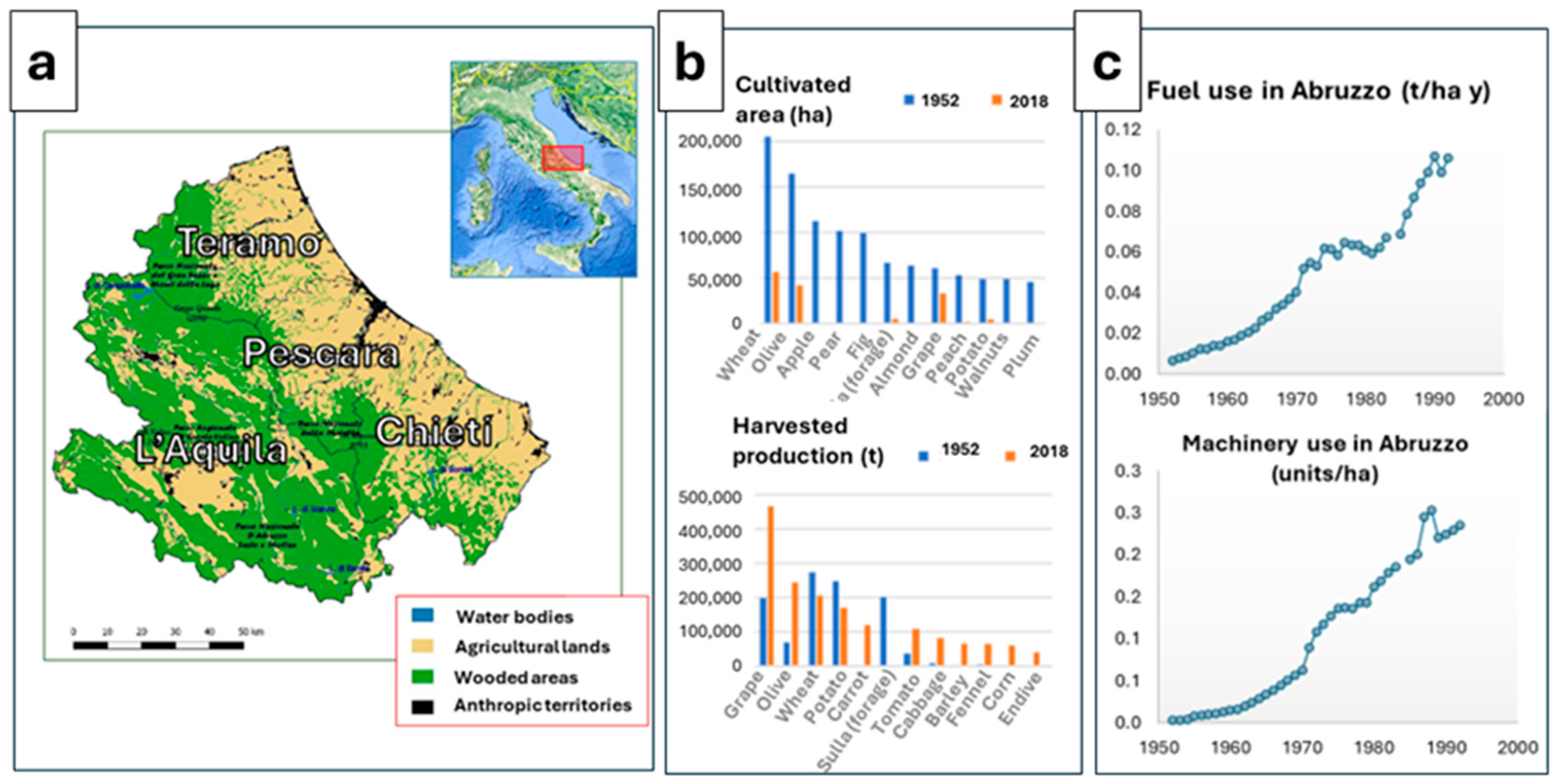
2.1. Geomorphology, Climate of the Study Area, and Crop Production Data

The Abruzzo region (central Italy, Figure 1a) includes four provinces, three of which (Chieti, Teramo, and Pescara) encompass both coastal and internal hilly/mountainous areas. L’Aquila province, situated furthest inland, exhibits the most complex geomorphology and climatic distribution. The current landscape results from tectonic activity that had a peak in the Neogene [45] and is still ongoing, together with seismic and ground deformation activity [46,47]. This geological history has shaped a complex orography with alternating NW–SE trending mountain ranges and valleys. Consequently, the region encompasses a wide altitudinal range, fostering a spectrum of climatic environments from coastal to high mountain. Two distinct climatic zones can be identified: the internal mountainous belt, characterized by complex topography and harboring diverse microclimates, with a prevailing continental regime featuring hot summers and cold winters and the external, hilly, and coastal range (Figure 1a), exhibiting a more uniform Mediterranean climate, with warm summers and mild winters.

The Abruzzo region boasts a well-established agricultural sector that has experienced significant growth in crop yields and production over the past six decades. Such production is primarily concentrated in coastal areas and inland plains and includes as the main crops, wheat, olive, and grape. An overall increase in harvest has been accompanied by a decrease in cultivated area for all crops over the past six decades (Figure 1b). This trend reflects a significant increase in crop yields, accompanied by substantial investments, as evidenced, by way of example, by the progressive increase in the use of agricultural machinery and fuels (Figure 1c).

Among the main crops cultivated in Abruzzo, wheat occupies the most extensive harvested area. Approximately three-quarters of the total regional production is concentrated in the provinces of Chieti and Teramo, while the production from the province of L’Aquila is practically marginal.

The crop production data involved in the present study are provided by the Italian National Institute of Statistics [48,49] and consist of a time series, in the time range 1952–2014, of the yearly values of harvested area and total production for wheat.

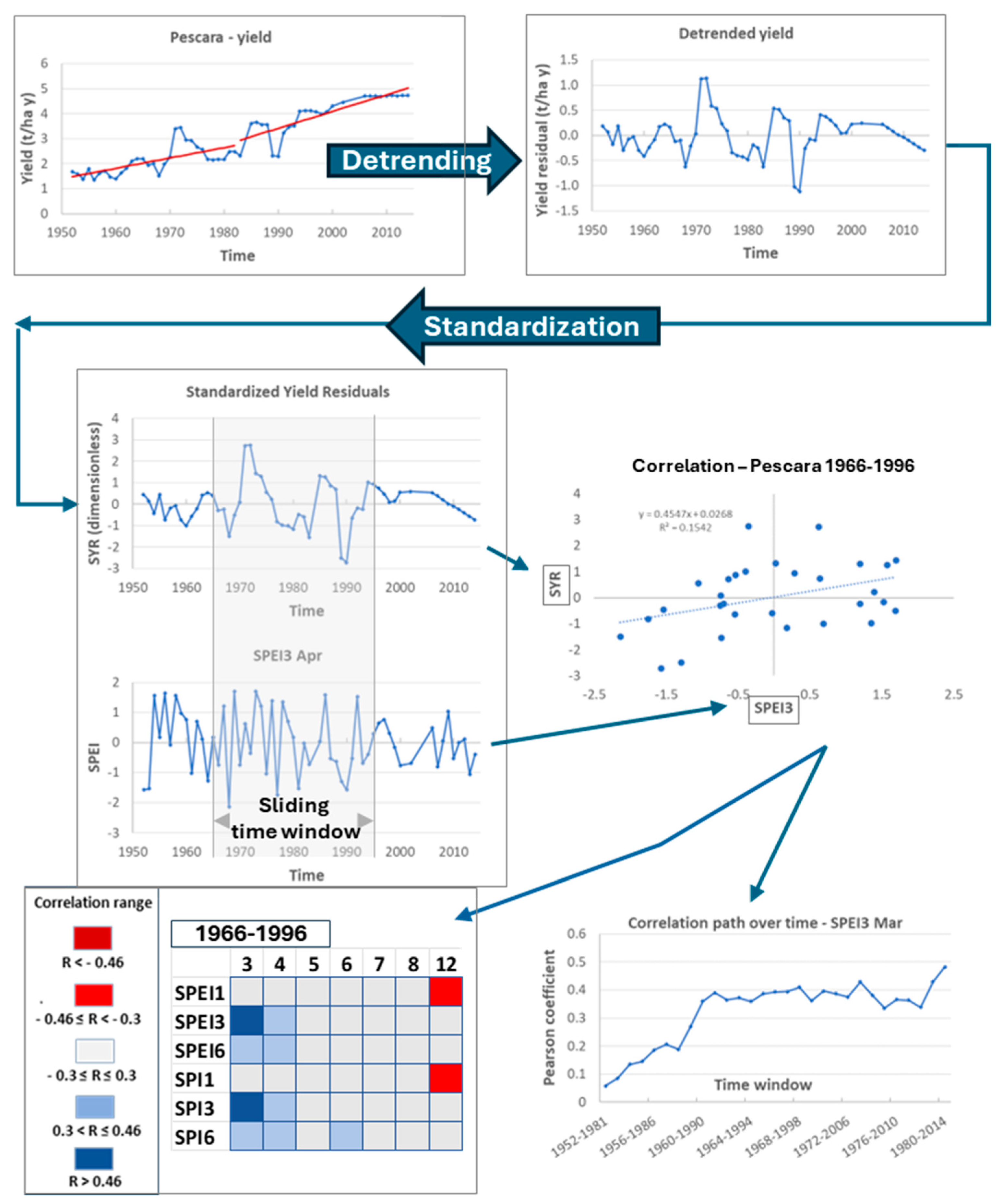
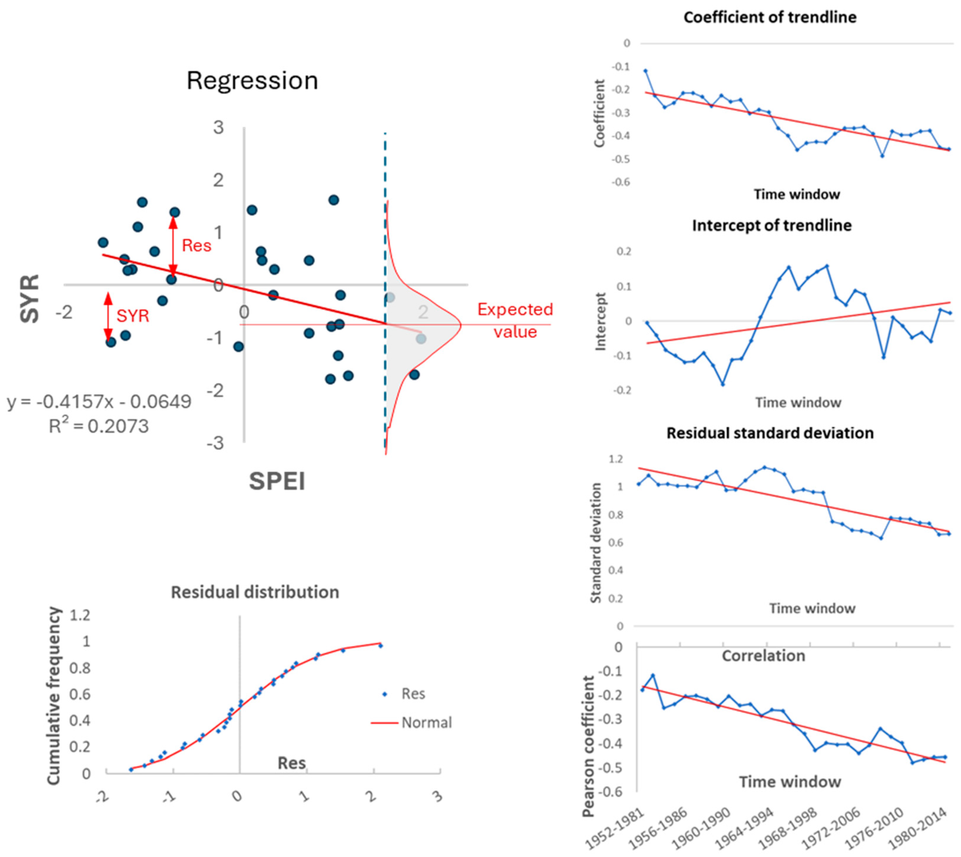
2.2. Joint Analysis of Thermo-Pluviometric and Crop Yield Time Series

The study of the response of the crop production system to climatic fluctuations, and how it varies in the long term, was conducted through correlation analysis between fluctuations in SPI/SPEI indices and fluctuations in wheat yield.

The meteorological and climatic data used to calculate the SPI and SPEI indices were gathered from the Hydrological Services of the Abruzzo and Campania regions [43,50,51] and consist of monthly and daily series of temperature and precipitation data, recorded in 37 stations distributed throughout the regional territory, in the time interval from 1952 to 2014.

SPI values were calculated over this interval using the free SPI_Generator v1.7.5 software [52], whereas SPEI values were calculated using the SPEI Calculator libraries of the R language [53]. Since SPI and SPEI are standardized indices, the crop yield data were also appropriately processed and standardized, according to the following steps. (i) Detrending: the deviations, or residuals, of the annual yield values from the increasing linear trends (least squares lines) were calculated, as the differences between measured yield and trend-predicted yield (Figure 2). As crop yield trends are presumably associated with yield increases due to non-climatic factors, e.g., mechanization, improvements in agronomic techniques, etc. (Section 2.1), detrending can enables isolation of the effect of climatic fluctuations. (ii) Standardization: for each residual value, denoted by r, the Standardized Yield Residual (SYR) is calculated using the standardized variable:

$$\mathrm{SYR}={\displaystyle \frac{\mathrm{r}-\mathsf{\mu }}{\mathsf{\sigma }}}$$

(1)

where μ and σ denote the mean and standard deviation of the residuals, respectively. Detrending and standardization were performed on the basis of the sub-trends, relative to the time intervals 1952–1982 and 1983–2014 for each province studied. The choice of these intervals is explained in detail in Section 3.1.

We then conducted, for each province, a time series regression analysis between SYR series and monthly, quarterly, and semi-annual SPI and SPEI indices (here denoted by SPI1, SPI3, and SPI6, respectively; the same applies to the SPEI indices), calculated for different months of the year. The analysis was repeated on time windows of approximately thirty years in width, sliding in the time interval from 1952 to 2014. Thus, the first time window covers the time range 1952–1981, the second the period 1953–1982, and so on. In this way, a time series of correlation coefficients is obtained for each index considered and for each province, which allows us to assess whether there is a systematic variation of the correlation coefficient over time. Figure 2 shows an example of data processing and the obtained time series, while the complete results achieved are illustrated and discussed in Section 3.

Since some data are missing in the crop yield data set (those for the years 1984, 2001, 2004, 2005), it was decided to extend the time window size, when necessary, in order to ensure all samples contained 30 elements. Thus, for example, the 1955–1984 window was extended to 1955–1985, since the 1984 datum was missing.

The statistical significance of the correlation was evaluated using Student’s t-test, with significance levels of 10% and 1%. For a statistical sample of 30 pairs of values (SYR, SPI) or (SYR, SPEI), these significance levels are associated with critical values (p-value), in absolute value, equal to 0.30 and 0.46, respectively. In simple terms, a correlation coefficient (in absolute value) greater than 0.30 indicates that there is a less than 10% probability that the two data series (e.g., SYR and SPEI) are actually uncorrelated and that the estimate obtained is due to a stochastic fluctuation of the estimator beyond this threshold. A value greater (in absolute value) than 0.46 indicates that the two series are truly correlated with extremely high probability and that the considered SPI or SPEI index significantly controls the deviation of crop yield from its trend.

For each time window and province, a panel was therefore constructed (Figure 2, bottom). Each cell within the panel corresponds to a specific SPI/SPEI index calculated for a particular month of the year (here the months of December and from March to August were considered). The cell color reflects the recorded significance level, as indicated by the legend in Figure 2. It is recalled that a positive correlation value (light or dark blue cell) or a negative one (light or dark red cell) does not denote a favorable or unfavorable impact of a particular index on crop yield. Instead, it signifies that, in the former case, drought is a limiting factor for yield, while in the latter case, an excessively humid climate is the constraining factor.

A sequence of such panels corresponding to consecutive time windows provides a wealth of valuable insights:

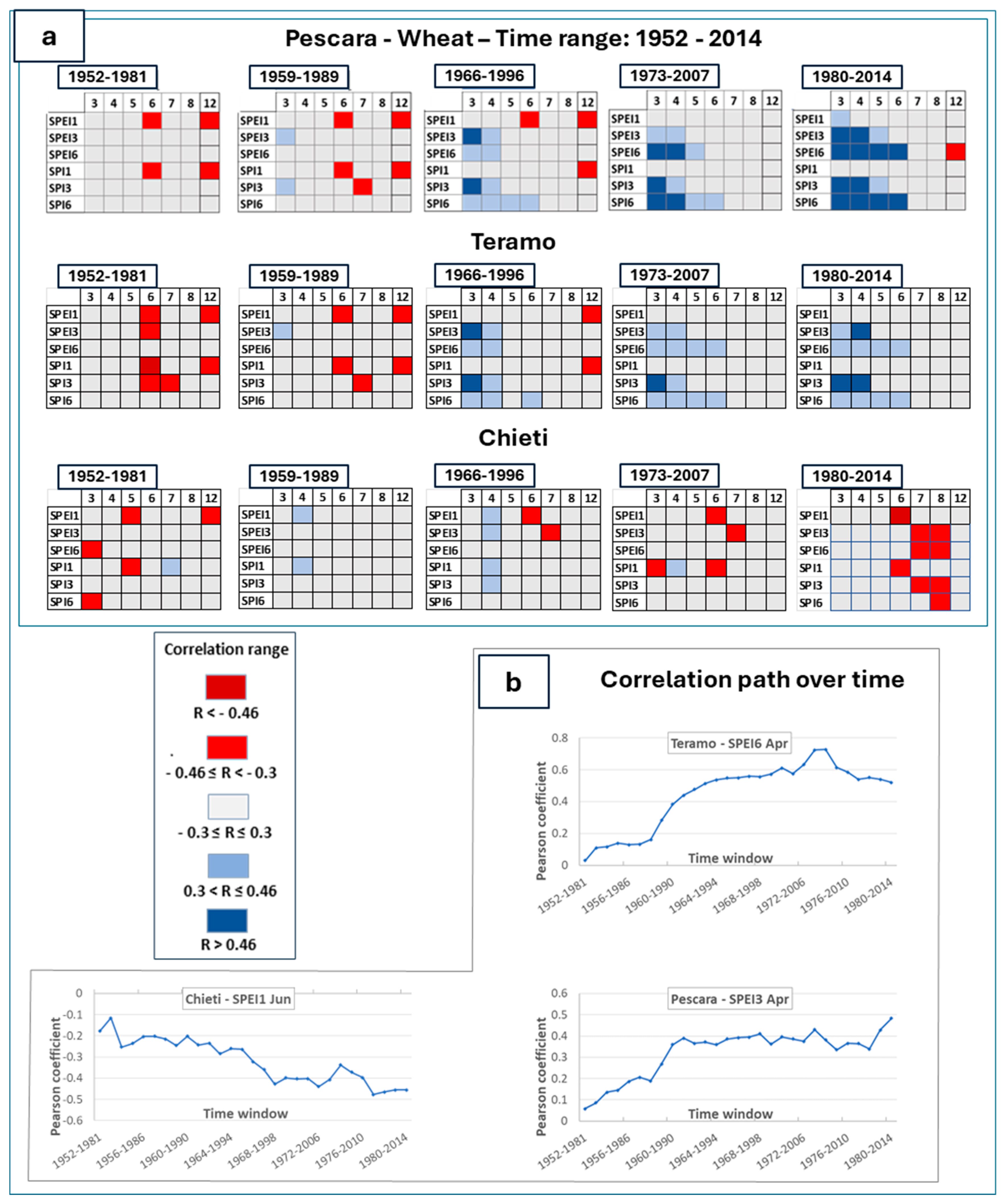
• Changing sensitivity to climate fluctuations: an overall increase (or decrease) in the number of colored cells and/or dark cells (blue or red) over time can be interpreted as an enhanced (or reduced) sensitivity of the crop production system to climatic fluctuations.
• Shifting vulnerabilities: the migration of colored cells from one area of the panel to another can shed light on the specific periods of the year or phenological stages that become increasingly important in terms of the climate vulnerability of yield.
• Identifying dominant drought indices: by examining the trend of correlation coefficients for the most impactful drought indices, the study can identify the indices that exhibit the most pronounced and consistent trends over time. These indices serve as valuable tools for monitoring and predicting climate-induced yield variations.

The trend analysis of identified dominant indices is the last phase of this study. The trend analysis of correlation coefficients uncovers crucial information in deciphering the temporal evolution of the climate–yield relationship.

3. Results and Discussion

3.1. Crop Yield Trends

During the six-decade period from 1952 to 2014, wheat yields exhibited an increasing trend, which can be further divided into two sub-trends for each province: (i) a trend associated with the first three decades, from 1952 to 1982, which is similar across all four provinces (Figure 3), with coefficients within the range 0.034–0.047; (ii) a trend in the second three decades, from 1983 to 2014, where the four provinces display substantially different behaviors. In the period following 2007, the provinces of Teramo (the region’s largest producer) and Pescara show a yield stabilization around a value of approximately 4.5 t/(ha y). Nevertheless, the 2007–2014 time range is too short to identify a definitive trend. Therefore, for this analysis, we consider the two aforementioned sub-trends, i.e., 1952–1982 and 1983–2014.

3.2. Correlation Analysis

The statistical analysis conducted revealed an overall intensification of the correlation between the SPI/SPEI drought indices and wheat yield (SYR) in the provinces of Teramo, Chieti, and Pescara, which account for nearly 95% of regional wheat production. Notably, for Teramo and Pescara, a progressive increase in the Pearson correlation coefficient was observed for the SPI/SPEI indices related the March–May period (Figure 4a). Conversely, a growing negative correlation (with an increasing absolute value of the coefficient) was observed for the indices of June and July for the province of Chieti.

The increasing correlation observed for the provinces of Teramo and Pescara suggests that drought during the winter–spring period is becoming a more significant limiting factor for wheat yield. This is highlighted by the diagram in Figure 4a, where the number of blue and dark blue colored cells progressively migrates towards the March–May spring period.

In the case of Chieti, the increasing negative correlation indicates that excessively humid conditions during the summer period are becoming a more prominent limiting factor for wheat yield. In Figure 4a, for Chieti, the red and dark red colored cells progressively concentrate in the June–August summer period.

The panels in Figure 4a provide a comprehensive overview of the temporal evolution of the correlation between drought indices and wheat yield fluctuations. Additionally, they enabled the identification of SPI/SPEI indices that exhibited the most pronounced correlation trends (Figure 4b).

The analysis highlighted that different provinces exhibit distinct behaviors (attributable to differences in climate, agricultural practices, etc.), even when geographically close or bordering each other. Notably, Teramo and Pescara show similar responses, while Chieti exhibits a substantially different behavior. Therefore, analyses conducted at the regional or sub-provincial scale may yield different results from those observed here. Consequently, the scale of observation should be carefully evaluated in this kind of statistical analysis.

Considering that Guerriero et al. [42] documented a climate transition from a temperate climate to a more arid condition during the 1952–2014 period across the study region, the observed increases in correlation can be interpreted as a characteristic of the climate adaption of the wheat production system. This adaptation has led to progressive increases in wheat yield but has not mitigated the impact of short-term climate fluctuations.

In other words, the Abruzzo wheat production system exhibits a growing sensitivity to climate fluctuations. The resulting production oscillations pose a potentially disturbing element to markets, leading to price volatility that is problematic for both food security and all economic stakeholders involved in the wheat production–consumption chain. Indeed, wheat price fluctuations can perturb the economic equilibria between producers, distributors, and consumers. Moreover, such volatility is typically accompanied by speculative phenomena and increased stockpiling, leading to an overall price increase [11].

The diagrams in Figure 4a are also useful for identifying, for each province, the periods of the year when the production system is most vulnerable and the corresponding phenological stages.

Besides providing insights into the trend of vulnerability of the wheat production system to climatic fluctuations, the illustrated statistical approach (applicable to any kind of crop) paves the way for developing statistical prediction models that can prove highly valuable for agricultural sector management, related investments, and financial applications.

4. Perspective for Future Research

The development of statistical models for predicting the agricultural yield based on climate indices holds huge potential for enhanced management of the agricultural sector, investments, and price fluctuations. While the construction of a comprehensive model falls beyond the scope of this study, we provide a brief outline of its application, considering a simple first-approximation model.

Consider the scatterplot in Figure 5 for the Chieti province covering the 1980–2014 time window, with SYR on the ordinate and monthly SPEI for June on the abscissa. For now, we adopt a simple linear regression model. Analyzing the residuals, denoted as Res (to distinguish them from SYR), allows us to determine their distribution, which in this case is well approximated by a normal distribution (Figure 5; residual distribution diagram). This also enables us to obtain an initial estimate of the standard deviation.

Knowledge of the regression line and the standard deviation of the residuals allows us to calculate the conditional probability distribution of the residuals Res, given that a climate index has reached a certain value. For instance, if the considered SPEI index assumes the value 1.5, the conditional probability distribution of SYR is a Gaussian distribution with mean given by the value provided by the regression line and variance estimated for the residuals Res (Figure 5).

Analyzing the temporal trend of the slope and intercept of the regression line, as well as the variance of the residuals (Res), allows us to calculate more accurate estimates of these parameters compared to those obtained from the scatterplot in Figure 5. This is because they are based on a larger dataset.

Once the conditional probability distribution of SYR is calculated, we can derive the probability distribution of the crop yield (non-standardized) residuals, and then of yield itself, by considering that from Equation (1):

r = SYR × σ + μ.

Then, the yield is estimated as the sum of the unstandardized residual r and the predicted yield value through the trend (Figure 5), so providing the yield conditional probability distribution.

The illustrated model can be adapted to use more realistic nonlinear interpolation curves (e.g., polynomials) to describe the yield–drought relationship (e.g., Potopova et al., 2016) or the temporal trend of certain parameters, such as crop yield.

Through this approach, we can estimate, by way of example, the probability that wheat production (or other crops) will be below or above a certain threshold, knowing that the SPI or SPEI index of a specific month has reached a certain value. This kind of prediction can have significant applications in both agricultural sector management and the economic and financial forecasting of agricultural products and derivatives prices at various scales of observation, from local to international. Furthermore, integrating economic factors, such as production costs and market dynamics, may provide a more holistic perspective on climate–agriculture dynamics, as well as provide a more comprehensive framework for decision making, and will be subject for future research.

5. Conclusions

The joint analysis of meteorological and crop yield data in the Abruzzo region revealed a trend of intensifying correlation between crop yield and drought indices (SPI and SPEI) during the 1952–2014 period. The main results of this study can be summarized as follows:

• The individuated correlation trends can be interpreted as a growing sensitivity of the Abruzzo wheat production system to climate fluctuations. The observed results provide a picture of the climate adaption characteristics of the wheat production system. This adaptation has led to progressive increases in wheat yield, but it has not mitigated the impact of short-term climate fluctuations.
• The dominant SPI and SPEI indices were identified for each wheat-producing province, further pinpointing the periods of the year and corresponding phenological stages when the production system appears most vulnerable.
• Different provinces have shown diverse responses over time, even if they are neighboring one another. Therefore, when designing this kind of analysis, the observation scale must be carefully evaluated.
• This study delves into the temporal dynamics of the wheat yield response to climate fluctuations in Abruzzo, offering valuable insights into the evolving climate–yield relationship.
• The statistical approach illustrated provides a robust framework for monitoring climate impacts on crop yields
• These results also provide the basis for developing predictive models to support informed decision making in agricultural management and financial planning.

References

1. Lobell, D.B.; Field, C.B. Global scale climate–crop yield relationships and the impacts of recent warming. Environ. Res. Lett. 2007, 2, 014002. [Google Scholar] [CrossRef]
2. Kang, Y.; Khan, S.; Ma, X. Climate change impacts on crop yield, crop water productivity and food security—A review. Prog. Nat. Sci. 2009, 19, 1665–1674. [Google Scholar] [CrossRef]
3. Deschênes, O.; Greenstone, M. Climate Change, Mortality, and Adaptation: Evidence from Annual Fluctuations in Weather in the US. Am. Econ. J. Appl. Econ. 2011, 3, 152–185. [Google Scholar] [CrossRef]
4. Deschênes, O.; Greenstone, M. The Economic Impacts of Climate Change: Evidence from Agricultural Output and Random Fluctuations in Weather: Reply. Am. Econ. Rev. 2012, 102, 3761–3773. [Google Scholar] [CrossRef]
5. Lobell, D.B.; Gourdji, S.M. The Influence of Climate Change on Global Crop Productivity. Plant Physiol. 2012, 160, 4. [Google Scholar] [CrossRef] [PubMed]
6. Segerstrom, T.M. Global Climate Change, Fair Trade, and Coffee Price Volatility. Gettysbg. Econ. Rev. 2016, 9, 6. Available online: https://cupola.gettysburg.edu/ger/vol9/iss1/6 (accessed on 18 July 2024).
7. Moore, F.C.; Baldos, U.L.; Hertel, T. Economic impacts of climate change on agriculture: A comparison of process-based and statistical yield models. Environ. Res. Lett. 2017, 12, 065008. [Google Scholar] [CrossRef]
8. Holleman, C.; Rembold, F.; Crespo, O.; Conti, V. The impact of climate variability and extremes on agriculture and food security—An analysis of the evidence and case studies. In Background Paper for The State of Food Security and Nutrition in the World 2018; FAO Agricultural Development Economics Technical Study No. 4; FAO: Rome, Italy, 2020. [Google Scholar] [CrossRef]
9. Abbass, K.; Qasim, M.Z.; Song, H.; Murshed, M.; Mahmood, H.; Younis, I. A review of the global climate change impacts, adaptation, and sustainable mitigation measures. Environ. Sci. Pollut. Res. 2022, 29, 42539–42559. [Google Scholar] [CrossRef] [PubMed]
10. IPCC. Summary for Policymakers. In Climate Change 2021: The Physical Science Basis; Contribution of Working Group I to the Sixth Assessment Report of the Intergovernmental Panel on Climate Change; Masson-Delmotte, V., Zhai, P., Pirani, A., Connors, S.L., Péan, C., Berger, S., Caud, N., Chen, Y., Goldfarb, L., Gomis, M.I., et al., Eds.; Cambridge University Press: Cambridge, UK, 2021. [Google Scholar]
11. Tran, A.N.; Welch, J.R.; Lobell, D.; Roberts, M.J.; Schlenker, W. Commodity prices and volatility in response to anticipated climate change. In Proceedings of the Annual Meeting of Agricultural & Applied Economics Association, Seattle, USA, 12–14 August 2012. [Google Scholar] [CrossRef]
12. Zhao, Y.; Chen, X.; Lobell, D.B. An approach to understanding persistent yield variation—A case study in North China Plain. Eur. J. Agron. 2016, 77, 10–19. [Google Scholar] [CrossRef]
13. Mazhar, N.; Sultan, M.; Amjad, D. Impacts of rainfall and temperature variability on wheat production in district Bahawalnagar, Pakistan from 1983–2016. Pak. J. Sci. 2020, 72, 4. [Google Scholar] [CrossRef]
14. Ostberg, S.; Schewe, J.; Childers, K.; Frieler, K. Changes in crop yields and their variability at different levels of global warming. Earth Syst. Dyn. 2018, 9, 2. [Google Scholar] [CrossRef]
15. Iizumi, T.; Ramankutty, N. Changes in yield variability of major crops for 1981–2010 explained by climate change. Environ. Res. Lett. 2016, 11, 034003. [Google Scholar] [CrossRef]
16. Meng, Q.; Chen, X.; Lobell, D.; Cui, Z.; Zhang, Y.; Yang, H.; Zhang, F. Growing sensitivity of maize to water scarcity under climate change. Sci Rep. 2016, 6, 19605. [Google Scholar] [CrossRef] [PubMed]
17. Lobell, D.B.; Roberts, M.J.; Schlenker, W.; Braun, N.; Little, B.B.; Rejesus, R.M.; Hammer, G.L. Greater Sensitivity to Drought Accompanies Maize Yield Increase in the U. S. Midwest. Sci. 2014, 344, 516–519. [Google Scholar] [CrossRef] [PubMed]
18. Lobell, D.B.; Deines, J.M.; Tommaso, S.D. Changes in the drought sensitivity of US maize yields. Nat. Food 2020, 1, 729–735. [Google Scholar] [CrossRef] [PubMed]
19. Palmer, W.C. Meteorological Drought; US Department of Commerce, Weather Bureau: Washington, DC, USA, 1965; Volume 30. [Google Scholar]
20. McKee, T.B.; Doesken, N.J.; Kleist, J. The relationship of drought frequency and duration to time scales. In Proceedings of the 8th Conference on Applied Climatology, Anaheim, CA, USA, 17–22 January 1993; Volume 17, No. 22. pp. 179–183. [Google Scholar]
21. Narasimhan, B.; Srinivasan, R. Development and evaluation of Soil Moisture Deficit Index (SMDI) and Evapotranspiration Deficit Index (ETDI) for agricultural drought monitoring. Agric. For. Meteorol. 2005, 133, 69–88. [Google Scholar] [CrossRef]
22. Vicente-Serrano, S.M.; Beguería, S.; López-Moreno, J.I. A Multiscalar Drought Index Sensitive to Global Warming: The Stand-ardized Precipitation Evapotranspiration Index. J. Clim. 2010, 23, 1696–1718. [Google Scholar] [CrossRef]
23. Gunst, L.; Rego, F.M.C.C.; Dias, S.M.A.; Bifulco, C.; Stagge, J.H.; Rocha, M.S.; Van Lanen, H.A.J. Links between Meteorological Drought Indices and Yields (1979–2009) of the Main European Crops; Technical Report No. 36; DROUGHT-R&SPI Project: Wa-geningen, The Netherlands, 2015. [Google Scholar]
24. World Meteorological Organization (WMO); Global Water Partnership (GWP). Handbook of Drought Indicators and Indices; Svoboda, M., Fuchs, B.A., Eds.; Integrated Drought Management Programme (IDMP), Integrated Drought Management Tools and Guidelines Series 2; World Meteorological Organization (WMO) and Global Water Partnership (GWP): Geneva, Switzerland, 2016; ISBN 978-92-63-11173-9. [Google Scholar]
25. Potopová, V.; Boroneanţ, C.; Boincean, B.; Soukup, J. Impact of agricultural drought on main crop yields in the Republic of Moldova. Int. J. Clim. 2016, 36, 2063–2082. [Google Scholar] [CrossRef]
26. Tian, L.; Yu an, S.; Quiring, S.M. Evaluation of six indices for monitoring agricultural drought in the south-central United States. Agric. For. Meteorol. 2018, 249, 107–119. [Google Scholar] [CrossRef]
27. Peña-Gallardo, M.; Vicente-Serrano, S.M.; Domínguez-Castro, F.; Beguería, S. The impact of drought on the productivity of two rainfed crops in Spain. Nat. Hazards Earth Syst. Sci. 2019, 19, 1215–1234. [Google Scholar] [CrossRef]
28. Peña-Gallardo, M.; Vicente-Serrano, S.M.; Domínguez-Castro, F.; Quiring, S.; Svoboda, M.; Beguería, S.; Hannaford, J. Effectiveness of drought indices in identifying impacts on major crops across the USA. Clim. Res. 2018, 75, 221–240. [Google Scholar] [CrossRef]
29. Bezdan, J.; Bezdan, A.; Blagojević, B.; Mesaroš, M.; Pejić, B.; Vranešević, M.; Pavić, D.; Nikolić-Đorić, E. SPEI-Based Approach to Agricultural Drought Monitoring in Vojvodina Region. Water 2019, 11, 1481. [Google Scholar] [CrossRef]
30. Di Lena, B.; Farinelli, D.; Palliotti, A.; Poni, S.; DeJong, T.M.; Tombesi, S. Impact of climate change on the possible expansion of almond cultivation area pole-ward: A case study of Abruzzo, Italy. J. Hortic. Sci. Biotechnol. 2018, 93, 209–215. [Google Scholar] [CrossRef]
31. Di Lena, B.; Curci, G.; Vergni, L.; Farinelli, D. Climatic Suitability of Different Areas in Abruzzo, Central Italy, for the Culti-vation of Hazelnut. Horticulturae 2022, 8, 580. [Google Scholar] [CrossRef]
32. Leff, B.; Ramankutty, N.; Foley, J.A. Geographic distribution of major crops across the world. Glob. Biogeochem. Cycle 2004, 18, GB1009. [Google Scholar] [CrossRef]
33. Food and Agriculture Organization FAOSTAT: Crops and Livestock Products. Available online: https://www.fao.org/faostat/en/#data/QCL/visualize. (accessed on 12 May 2024).
34. Tuel, A.; Eltahir, E.A. Why is the Mediterranean a climate change hot spot? J. Clim. 2020, 33, 5829–5843. [Google Scholar] [CrossRef]
35. Giorgi, F.; Lionello, P. Climate change projections for the Mediterranean region. Glob. Planet. Chang. 2008, 63, 90–104. [Google Scholar] [CrossRef]
36. Scorzini, A.R.; Leopardi, M. Precipitation and temperature trends over central Italy (Abruzzo Region): 1951–2012. Theor. Appl. Clim. 2018, 135, 959–977. [Google Scholar] [CrossRef]
37. Michaelides, S.; Karacostas, T.; Sánchez, J.L.; Retalis, A.; Pytharoulis, I.; Homar, V.; Romero, R.; Zanis, P.; Giannakopoulos, C.; Bühl, J.; et al. Reviews and perspectives of high impact atmospheric processes in the Mediterranean. Atmos. Res. 2018, 208, 4–44. [Google Scholar] [CrossRef]
38. Fioravanti, G.; Piervitali, E.; Desiato, F. A new homogenized daily data set for temperature variability assessment in Italy. Int. J. Clim. 2019, 39, 5635–5654. [Google Scholar] [CrossRef]
39. Aruffo, E.; Di Carlo, P. Homogenization of instrumental time series of air temperature in Central Italy (1930–2015). Clim. Res. 2019, 77, 193–204. [Google Scholar] [CrossRef]
40. Caporali, E.; Lompi, M.; Pacetti, T.; Chiarello, V.; Fatichi, S. A review of studies on observed precipitation trends in Italy. Int. J. Climatol. 2021, 41, E1–E25. [Google Scholar] [CrossRef]
41. Curci, G.; Guijarro, J.A.; Di Antonio, L.; Di Bacco, M.; Di Lena, B.; Scorzini, A.R. Building a local climate reference dataset: Application to the Abruzzo region (Central Italy), 1930–2019. Int. J. Clim. 2021, 41, 4414–4436. [Google Scholar] [CrossRef]
42. Guerriero, V.; Scorzini, A.R.; Di Lena, B.; Iulianella, S.; Di Bacco, M.; Tallini, M. Impact of Climate Change on Crop Yields: Insights from the Abruzzo Region, Central Italy. Sustainability 2023, 15, 14235. [Google Scholar] [CrossRef]
43. Mann, H.B. Non-Parametric Test against Trend. Econometrica 1945, 13, 245–259. [Google Scholar] [CrossRef]
44. Péguy, C.P. Précis de Climatologie, 2nd ed.; Masson: Paris, France, 1970; 468p. [Google Scholar]
45. Cosentino, D.; Asti, R.; Nocentini, M.; Gliozzi, E.; Kotsakis, T.; Mattei, M.; Esu, D.; Spadi, M.; Tallini, M.; Cifelli, F.; et al. New insights into the onset and evolution of the central Apennine extensional intermontane basins based on the tectonically active L’Aquila Basin (central Italy). Bull. Geol. Soc. Am. 2017, 129, 1314–1336. [Google Scholar] [CrossRef]
46. Sciortino, A.; Marini, R.; Guerriero, V.; Mazzanti, P.; Spadi, M.; Tallini, M. Satellite A-DInSAR pattern recognition for seismic vulnerability mapping at city scale: Insights from the L’Aquila (Italy) case study. GISci. Remote Sens. 2024, 61, 1. [Google Scholar] [CrossRef]
47. Sciortino, A.; Guerriero, V.; Marini, R.; Spadi, M.; Mazzanti, P.; Tallini, M. Geological and Hydrogeological Drivers of Seismic Deformation in L’Aquila, Italy: Insights from InSAR Analysis. Geomat. Nat. Hazards Risk 2024, 15, 2362395. [Google Scholar] [CrossRef]
48. ISTAT, Biblioteca Digitale-Annuario di Statistica Agraria. Available online: https://ebiblio.istat.it/SebinaOpac/resource/annuario-di-statistica-agraria/IST0010796 (accessed on 15 August 2023).
49. ISTAT, Dati-Agricoltura-Coltivazioni-Superfici e Produzione. Available online: http://dati.istat.it (accessed on 15 August 2023).
50. Annali Idrologici della Regione Abruzzo, Ufficio Idrografico e Mareografico—Pescara. Available online: https://www.regione.abruzzo.it/content/annali-idrologici?page=2 (accessed on 15 August 2023).
51. Annali Idrologici della Regione Campania, Centro Funzionale Multirischi della Protezione Civile Regione Campania, Annali Idrologici e Altre Pubblicazioni del Compartimento di Napoli del S.I.M.N. Available online: http://centrofunzionale.regione.campania.it/#/pages/documenti/annali (accessed on 15 August 2023).
52. National Drought Mitigation Center SPI Generator [Software]. University of Nebraska–Lincoln. 2018. Available online: https://drought.unl.edu/Monitoring/SPI/SPIProgram.aspx (accessed on 12 May 2024).
53. Begueria, S.; Vicente-Serrano, S.M. SPEI Calculator. 2009. Available online: http://hdl.handle.net/10261/10002 (accessed on 12 May 2024).
Figure 1. (a) Land use in the studied provinces of the Abruzzo region, central Italy; (b) comparison between harvested production and cultivated area for the main crops in Abruzzo in 1952 and 2018; and (c) trend of mechanization and fuel use in the studied region between the 1950s and 1990s.
Sustainability 16 06462 g001
Figure 2. Phases of the illustrated statistical analysis. Residual standardization provides a dimensionless variable for which the correlation with the SPI and SPEI indices of different periods and months of the year is estimated along time windows of thirty years in width, sliding within the time range from 1952 to 2014. The scatterplot illustrates an example of the regression analysis of SYR vs. SPEI3 of March, over the time window 1966–1996. The panel at the bottom summarizes the correlation values estimated for several months of the year (denoted by the column number). The colored cells denote correlation coefficients, in absolute value, above the thresholds of 0.3 and 0.46, which are associated with levels of significance of 10% and 1%, respectively (see main text). The diagram in the bottom right illustrates the correlation values estimated for the dominant SPEI index (here SPEI3 of March) over all time windows.
Sustainability 16 06462 g002
Figure 3. Wheat crop yield in the studied provinces, with related trends.
Sustainability 16 06462 g003
Figure 4. Results of the correlation analysis conducted over sliding time windows over the time range 1952–2014. (a) Tables of significant correlation coefficients estimated over five different time windows (see main text). The symbols SPI1, SPI3, and SPI6 denote monthly, quarterly, and semi-annual SPI respectively; the same applies to the SPEI indices. The column number denotes the month in which SPI/SPEI are calculated. (b) Path of the correlation coefficients for the dominant SPEI indices, identified by means of the tables in panel (a).
Sustainability 16 06462 g004
Figure 5. Forecasting model. In the regression scatterplot each SPEI value is associated with a conditioned probability distribution of SYR (denoted by the shaded area). The comparison between the residual distribution of Res (diagram at the bottom) and the normal model ensures that this latter provides a good approximation for Res distribution. The SYR conditional probability distribution shows the same variance of Res and average given by the expected value associated with each SPEI value.
Sustainability 16 06462 g005
Disclaimer/Publisher’s Note: The statements, opinions and data contained in all publications are solely those of the individual author(s) and contributor(s) and not of MDPI and/or the editor(s). MDPI and/or the editor(s) disclaim responsibility for any injury to people or property resulting from any ideas, methods, instructions or products referred to in the content.